Error bound of critical points and KL property of exponent $1/2$ for squared F-norm regularized factorization

Abstract

This paper is concerned with the squared F(robenius)-norm regularized factorization form for noisy low-rank matrix recovery problems. Under a suitable assumption on the restricted condition number of the Hessian for the loss function, we derive an error bound to the true matrix for the non-strict critical points with rank not more than that of the true matrix. Then, for the squared F-norm regularized factorized least squares loss function, under the noisy and full sample setting we establish its KL property of exponent $1/2$ on its global minimizer set, and under the noisy and partial sample setting achieve this property for a class of critical points. These theoretical findings are also confirmed by solving the squared F-norm regularized factorization problem with an accelerated alternating minimization method.

Keywords: F-norm regularized factorization; error bound; KL property of exponent $1/2$

1 Introduction

Low-rank matrix recovery problems aim at recovering a true but unknown low-rank matrix $M^{*}\!\in\mathbb{R}^{n\times m}$ from as few observations as possible, and have wide applications in a host of fields such as statistics, control and system identification, signal and image processing, machine learning, quantum state tomography, and so on (see, e.g., [11, 10, 14, 25]). Generally, when a tight upper bound, say an integer $r\geq 1$, is available for the rank $r^{*}$ of $M^{*}$, they can be formulated as the rank constrained optimization problem

$$\min_{X\in\mathbb{R}^{n\times m}}\big{\{}f(X)\ \ {\rm s.t.}\ \ {\rm rank}(X)\leq r\big{\}}$$ (1)

where $f\!:\mathbb{R}^{n\times m}\rightarrow\mathbb{R}_{+}$ is an empirical loss function. Otherwise, one needs to solve a sequence of rank constrained optimization problems with an adjusted upper estimation for $r^{*}$. For the latter scenario, one may consider the rank regularized model

$$\min_{X\in\mathbb{R}^{n\times m}}\big{\{}f(X)+\lambda\,{\rm rank}(X)\big{\}}$$ (2)

with an appropriate $\lambda>0$ to achieve a desirable low-rank solution. Model (1)-(2) reduce to the rank constrained and regularized least squares problem, respectively, when

$$f(X):=\frac{1}{2}\|\mathcal{A}(X)-y\|^{2}\quad\ \forall X\in\mathbb{R}^{n\times m},$$ (3)

where $\mathcal{A}\!:\mathbb{R}^{n\times m}\rightarrow\mathbb{R}^{p}$ is the sampling operator and $y$ is the noisy observation from

$$y=\mathcal{A}(M^{*})+\omega.$$ (4)

Due to the combinatorial property of the rank function, rank optimization problems are NP-hard and it is impossible to seek a global optimal solution with a polynomial-time algorithm. A common way to deal with them is to adopt the convex relaxation technique. For the rank regularized problem (2), the popular nuclear norm relaxation method (see, e.g., [11, 25, 6]) yields a desirable solution via a single convex minimization problem

$$\min_{X\in\mathbb{R}^{n\times m}}\big{\{}f(X)+\lambda\|X\|_{*}\big{\}}.$$ (5)

Over the past decade active research, this method has made great progress in theory (see, e.g., [6, 7, 25, 20]). Despite its favorable performance in theory, improving computational efficiency remains a challenge. In fact, almost all convex relaxation algorithms for (2) require an economic SVD of a full matrix in each iteration, which forms the major computational bottleneck and restricts their scalability to large-scale problems. Inspired by this, recent years have witnessed the renewed interest in the Burer-Monteiro factorization [3] for low-rank matrix optimization problems. By replacing $X$ with its factored form $UV^{\mathbb{T}}$ for $(U,V)\in\!\mathbb{R}^{n\times r}\times\mathbb{R}^{n\times r}$ with $r^{*}\leq r<\min(n,m)$, the factored form of (5) is

$$\min_{U\in\mathbb{R}^{n\times r},V\in\mathbb{R}^{m\times r}}\Big{\{}\Phi_{\lambda}(U,V):=f(UV^{\mathbb{T}})+\frac{\lambda}{2}\big{(}\|U\|_{F}^{2}+\|V\|_{F}^{2}\big{)}\Big{\}}.$$ (6)

Although the factorization form tremendously reduces the number of optimization variables since $r$ is usually much smaller than $\min(n,m)$, the intrinsic bi-linearity makes the factored objective functions nonconvex and introduces additional critical points that are not global optimizers of factored optimization problems. A research line for factored optimization problems focuses on the nonconvex geometry landscape, especially the strict saddle property (see, e.g., [8, 12, 13, 19, 39, 40, 24, 29, 18, 17]). Most of these works center around the factorized forms of problem (1) or their regularized forms with a balanced term except [19] in which, under a restricted well-conditioned assumption on $f$, the authors proved that every critical point $(\overline{U},\overline{V})$ of problem (6) with $r\geq{\rm rank}(X^{*})$, where $X^{*}$ is an optimal solution of (5), either corresponds to a factorization of $X^{*}$ (i.e., $X^{*}=\overline{U}\overline{V}^{\mathbb{T}}$) or is a strict saddle point (i.e., the critical point at which the Hessian matrix has a strictly negative eigenvalue). This, along with the equivalence between (5) and (6) (see Lemma 1 in Appendix C) and the result of [17], implies that many local search algorithms such as gradient descent and its variants can find a global optimal solution of (6) with a high probability if the parameter $\lambda$ is chosen such that (5) has a solution with rank at most $r$. Another research line considers the (regularized) factorizations of rank optimization problems from a local view, and aims to characterize the convergence rate of the iterates in terms of a certain measure or the growth behavior of objective functions around the set of global optimal solutions (see, e.g., [16, 23, 30, 32, 36, 37, 38]).

For problem (1) associated to noisy low-rank matrix recovery, some researchers are also interested in the error bound to the true $M^{*}$ for the local optimizers of the factorization or its regularized form with a balanced term. For example, for the noisy low-rank positive semidefinite (PSD) matrix recovery, Bhojanapalli et al. [2] achieved the error bound for any local optimizer of the factorized exact or over-parameterization (i.e., $r\!\geq r^{*}$) under a RIP condition on the sampling operator; and for a general noisy low-rank matrix recovery, Zhang et al. [35] established the error bound for any local optimizer of the factorized exact-parameterization with a balanced regularization term under a restricted strong convexity and smoothness condition of the loss function. However, there are few works to discuss the error bounds for the critical point of the factorization associated to the rank regularized problem (2) or its convex relaxation (5) except [4] in which, for noisy matrix completion, the nonconvex Burer-Monteiro approach is used to show that the convex relaxation approach achieves near-optimal estimation errors.

This work is concerned with the error bound for the critical point of the nonconvex factorization (6) with $r\geq r^{*}$ and the KL property of exponent $1/2$ of $\Phi_{\lambda}$ associated to $r=r^{*}$ under the noisy setting. Specifically, under a suitable assumption on the restricted condition number of the Hessian matrix $\nabla^{2}f$, we derive an error bound to the true $M^{*}$ for those non-strict critical points with rank at most $r^{*}$, which is demonstrated to be optimal in terms of the exact characterization of global optimal solutions under the ideal noiseless and full sampling setting (see [36]). Different from [4], our error bound result is obtained for a general smooth loss by adopting a deterministic rather than probability analysis technique. In addition, for the least squares loss, under the noisy and full sample setting we establish the KL property of exponent $1/2$ of $\Phi_{\lambda}$ associated to almost all $\lambda>0$ over its global minimizer set, and under the noisy and partial sampling setup, achieve this property of $\Phi_{\lambda}$ only for a class of critical points. This extends the result of [36, Theorem 2] to the noisy setting. Together with the strict saddle property of $\Phi_{\lambda}$ in [19] and the result of [17], this means that for problem (6) with the least squares loss in the full sampling, many first-order methods can find a global optimal solution in a linear convergence rate with a high probability, provided that the parameter $\lambda$ is chosen such that (5) has an optimal solution with rank at most $r$. Hence, it partly improve the convergence analysis results of the alternating minimization methods proposed in [25, 15] for solving this class of problems. Li et al. [19] ever mentioned that the explicit convergence rate for some algorithms in [12, 29] can be obtained by extending the strict saddle property with the similar analysis in [40], but to the best of our knowledge, there is no strict proof for this, and the analysis in [40] is tailored to the factorization form with a balanced term.

Notation: Throughout this paper, $\mathbb{R}^{n\times m}$ represents the vector space of all $n\times m$ real matrices, equipped with the trace inner product $\langle X,Y\rangle={\rm trace}(X^{\mathbb{T}}Y)$ for $X,Y\in\mathbb{R}^{n\times m}$ and its induced F-norm, and we stipulate $n\leq m$. The notation $\mathbb{O}^{n\times\kappa}$ denotes the set of $n\times\kappa$ matrices with orthonormal columns, and $\mathbb{O}^{n}$ stands for $\mathbb{O}^{n\times n}$. Let $I$ denote an identity matrix whose dimension is known from the context. For a matrix $X\in\mathbb{R}^{n\times m}$, we denote by $\sigma(X)$ the singular value vector of $X$ arranged in a nonincreasing order, and by $\sigma^{\kappa}(X)$ for an integer $\kappa\geq 1$ the vector consisting of the first $\kappa$ entries of $\sigma(X)$, and write $X_{+}:=\max(0,X)$ and $\mathbb{O}^{n,m}(X):=\big{\{}(P,Q)\in\mathbb{O}^{n}\times\mathbb{O}^{m}\ |\ X=P{\rm Diag}(\sigma(X))Q^{\mathbb{T}}\big{\}},$ where ${\rm Diag}(z)$ represents a rectangular diagonal matrix with $z$ as the diagonal vector. We denote by $\|X\|$ and $\|X\|_{*}$ the spectral norm and the nuclear norm of $X$, respectively, by $X^{\dagger}$ the pseudo-inverse of $X$, and by ${\rm col}(X)$ the column space of $X$. Let $\mathcal{P}_{\rm on}$ and $\mathcal{P}_{\rm off}$ denote the linear mapping from $\mathbb{R}^{(n+m)\times(n+m)}$ to itself, respectively, defined by

$$\mathcal{P}_{\rm on}\Big{(}\left[\begin{matrix}A_{11}&A_{12}\\ A_{21}&A_{22}\end{matrix}\right]\Big{)}=\left[\begin{matrix}A_{11}&0\\ 0&A_{22}\\ \end{matrix}\right],\,\mathcal{P}_{\rm off}\Big{(}\left[\begin{matrix}A_{11}&A_{12}\\ A_{21}&A_{22}\end{matrix}\right]\Big{)}=\left[\begin{matrix}0&A_{12}\\ A_{21}&0\\ \end{matrix}\right]$$ (7)

where $A_{11}\in\mathbb{R}^{n\times n}$ and $A_{22}\in\mathbb{R}^{m\times m}$. For a given matrix pair $(U,V)\in\mathbb{R}^{n\times\kappa}\times\mathbb{R}^{m\times\kappa}$, we denote by $\mathbb{B}((U,V),\delta)$ the closed F-norm ball of radius $\delta$ centered at $(U,V)$, and by ${\rm dist}((U,V),\Gamma)$ the F-norm distance of $(U,V)$ from a set $\Gamma\subseteq\mathbb{R}^{n\times\kappa}\times\mathbb{R}^{m\times\kappa}$, and write

$$W=(U;V)\in\mathbb{R}^{(n+m)\times\kappa}\ \ {\rm and}\ \ \widehat{W}=(U;-V)\in\mathbb{R}^{(n+m)\times\kappa}.$$ (8)

We denote by $M^{*}$ the true matrix of rank $r^{*}$ with $4r^{*}\leq\min(m,n)$, and write

$$\mathcal{E}^{*}:=\Big{\{}\big{(}P_{1}^{*}{\Sigma^{*}}^{1/2}R,Q_{1}^{*}{\Sigma^{*}}^{1/2}R\big{)}\,|\,(P^{*},Q^{*})\in\mathbb{O}^{n,m}(M^{*}),R\in\mathbb{O}^{r^{*}}\Big{\}}$$

where $\Sigma^{*}={\rm Diag}(\sigma_{1}(M^{*}),\ldots,\sigma_{r^{*}}(M^{*}))\in\mathbb{R}^{r^{*}\times r^{*}}$, and $P_{1}^{*}$ and $Q_{1}^{*}$ are the matrix consisting of the first $r^{*}$ columns of $P^{*}$ and $Q^{*}$, respectively. For a given $U\in\mathbb{R}^{n\times\kappa}$, we also write $U=(U_{1};U_{2})$ where $U_{1}$ and $U_{2}$ are the matrix consisting of the first $r^{*}$ rows and the rest $n-r^{*}$ rows of $U$. For any given $A,B\in\mathbb{R}^{n\times\kappa}$, define ${\rm dist}(A,B):=\mathop{\min}_{R\in\mathbb{O}^{\kappa}}\|A-BR\|_{F}.$

2 Preliminaries

2.1 Restricted strong convexity and smoothness

Restricted strong convexity (RSC) and restricted smoothness (RSS) are the common requirement for loss functions when handling low-rank matrix recovery problems (see, e.g., [20, 21, 19, 40, 35]). Next we recall the concepts of RSC and RSS used in this paper.

Definition 2.1

A twice continuously differentiable function $\Psi\!:\mathbb{R}^{n\times m}\to\mathbb{R}$ is said to satisfy the $(\kappa,\kappa)$-RSC of modulus $\alpha$ and the $(\kappa,\kappa)$-RSS of modulus $\beta$, respectively, if $0<\alpha\leq\beta$ and for any $X,H\in\mathbb{R}^{n\times m}$ with ${\rm rank}(X)\leq\kappa$ and ${\rm rank}(H)\leq\kappa$,

$$\alpha\|H\|^{2}_{F}\leq\nabla^{2}\Psi(X)(H,H)\leq\beta\|H\|^{2}_{F}.$$ (9)

For the least squares loss in (3), the $(\kappa,\kappa)$-RSC of modulus $\alpha$ and $(\kappa,\kappa)$-RSS of modulus $\beta$ reduces to the $\kappa$-restricted smallest and largest eigenvalue of $\mathcal{A}^{*}\mathcal{A}$, i.e.,

$$0<\alpha=\min_{{\rm rank}(X)\leq\kappa,\|X\|_{F}=1}\|\mathcal{A}(X)\|^{2}\ \ {\rm and}\ \ \beta=\max_{{\rm rank}(X)\leq\kappa,\|X\|_{F}=1}\|\mathcal{A}(X)\|^{2}.$$

Consequently, the $(\kappa,\kappa)$-RSC of modulus $\alpha=1-\delta_{\kappa}$ along with the $(\kappa,\kappa)$-RSS of modulus $\beta\!=1+\delta_{\kappa}$ for some $\delta_{\kappa}\in(0,1)$ reduces to the RIP condition of the operator $\mathcal{A}$. From [25], the least squares loss associated to many types of random sampling operators satisfy this property with a high probability. In addition, from the discussions in [39, 19], some loss functions definitely have this property such as the weighted PCAs with positive weights, the noisy low-rank matrix recovery with noise matrix obeying Subbotin density [28, Example 2.13], or the one-bit matrix completion with full observations.

The following lemma improves a little the result of [19, Proposition 2.1] that requires $\Psi$ to have the $(2\kappa,4\kappa)$-RSC of modulus $\alpha$ and the $(2\kappa,4\kappa)$-RSS of modulus $\beta$.

Lemma 2.1

Let $\Psi\!:\mathbb{R}^{n\times m}\to\mathbb{R}$ be a twice continuously differentiable function satisfying the $(\kappa,\kappa)$-RSC of modulus $\alpha$ and the $(\kappa,\kappa)$-RSS of modulus $\beta$. Then, for any $X\in\!\mathbb{R}^{n\times m}$ with ${\rm rank}(X)\leq\kappa$ and any $Y,Z\in\!\mathbb{R}^{n\times m}$ with ${\rm rank}([Y\ \ Z])\leq\kappa$,

$$\Big{|}\frac{2}{\alpha+\beta}\nabla^{2}\Psi(X)(Y,Z)-\langle Y,Z\rangle\Big{|}\leq\frac{\beta-\alpha}{\alpha+\beta}\big{\|}Y\big{\|}_{F}\big{\|}Z\big{\|}_{F}.$$

Proof: Fix an arbitrary $(Y,Z)\in\mathbb{R}^{n\times m}\times\mathbb{R}^{n\times m}$ with ${\rm rank}([Y\ Z])\leq\kappa$. Fix any $X\in\mathbb{R}^{n\times m}$ with ${\rm rank}(X)\leq\kappa$. If one of $Y$ and $Z$ is the zero matrix, the result is trivial. So, we assume that $Y\neq 0$ and $Z\neq 0$. Write $\overline{Y}:=\frac{Y}{\|Y\|_{F}}$ and $\overline{Z}:=\frac{Z}{\|Z\|_{F}}$. Notice that ${\rm rank}([\overline{Y}\ \ \overline{Z}])\leq\kappa$ and ${\rm rank}(\overline{Y}\pm\overline{Z})\leq{\rm rank}([\overline{Y}\ \ \overline{Z}])$. Then, we have

$$\alpha\|\overline{Y}+\overline{Z}\|_{F}^{2}\leq\nabla^{2}\Psi(X)\big{(}\overline{Y}+\overline{Z},\overline{Y}+\overline{Z}\big{)}\leq\beta\big{\|}\overline{Y}+\overline{Z}\|_{F}^{2},$$

$$\alpha\|\overline{Y}-\overline{Z}\|_{F}^{2}\leq\nabla^{2}\Psi(X)\big{(}\overline{Y}-\overline{Z},\overline{Y}-\overline{Z}\big{)}\leq\beta\big{\|}\overline{Y}-\overline{Z}\|_{F}^{2}.$$

Along with $4|\nabla^{2}\Psi(X)\big{(}\overline{Y},\overline{Z}\big{)}|=\big{|}\nabla^{2}\Psi(X)(\overline{Y}\!+\!\overline{Z},\overline{Y}\!+\!\overline{Z})-\nabla^{2}\Psi(X)\big{(}\overline{Y}\!-\!\overline{Z},\overline{Y}\!-\!\overline{Z}\big{)}\big{|}$,

$$4\nabla^{2}\Psi(X)\big{(}\overline{Y},\overline{Z}\big{)}\leq\beta\big{\|}\overline{Y}+\overline{Z}\|_{F}^{2}-\alpha\|\overline{Y}-\overline{Z}\|_{F}^{2}=2(\beta-\alpha)+2(\beta+\alpha)\big{\langle}\overline{Y},\overline{Z}\big{\rangle},$$

$$-4\nabla^{2}\Psi(X)\big{(}\overline{Y},\overline{Z}\big{)}\leq\beta\big{\|}\overline{Y}-\overline{Z}\|_{F}^{2}-\alpha\big{\|}\overline{Y}+\overline{Z}\|_{F}^{2}=2(\beta-\alpha)-2(\beta+\alpha)\big{\langle}\overline{Y},\overline{Z}\big{\rangle}.$$

The last two inequalities imply the desired inequality. The proof is then completed. $\Box$

From the reference [33], we recall that a random variable $\xi$ is called sub-Gaussian if

$$K=\sup_{q\geq 1}q^{-1/2}(\mathbb{E}|\xi|^{q})^{1/q}<\infty,$$

and $K$ is referred to as the sub-Gaussian norm of $\xi$. Equivalently, the sub-Gaussian random variable $\xi$ satisfies the following bound for a constant $\tau^{2}$:

$$\mathbb{P}\big{\{}|\xi|>t\big{\}}\leq 2e^{-t^{2}/(2\tau^{2})}\ \ {\rm for\ all}\ t>0.$$ (12)

We call the smallest $\tau^{2}$ satisfying (12) the sub-Gaussian parameter. The tail-probability characterization in (12) enables us to define centered sub-Gaussian random vectors.

Definition 2.2

(see [5]) A random vector $w=(w_{1},\ldots,w_{p})^{\mathbb{T}}$ is said to be a centered sub-Gaussian random vector if there exists $\tau>0$ such that for all $t>0$ and all $\|v\|=1$,

$$\mathbb{P}\big{\{}|v^{\mathbb{T}}w|>t\big{\}}\leq 2e^{-t^{2}/(2\tau^{2})}.$$

2.2 Properties of critical points of $\Phi_{\lambda}$

To give the gradient and Hessian matrix of $\Phi_{\lambda}$, define $\Xi\!:\mathbb{R}^{n\times m}\to\mathbb{R}^{(n+m)\times(n+m)}$ by

$$\Xi(X):=\left(\begin{matrix}\lambda I&\nabla\!f(X)\\ \nabla\!f(X)^{\mathbb{T}}&\lambda I\\ \end{matrix}\right).$$ (13)

For any given $(U,V)\in\mathbb{R}^{n\times r}\times\mathbb{R}^{m\times r}$, the gradient of $\Phi_{\lambda}$ at $(U,V)$ takes the form of

$$\nabla\Phi_{\lambda}(U,V)=\left[\begin{matrix}\nabla\!f(X)V+\lambda{U}\\ \nabla\!f(X)^{\mathbb{T}}{U}+\lambda{V}\end{matrix}\right]=\Xi(X)W\ \ {\rm with}\ \ X=UV^{\mathbb{T}};$$ (14)

and for any $\Delta=(\Delta_{U};\Delta_{V})$ with $\Delta_{U}\in\mathbb{R}^{n\times r}$ and $\Delta_{V}\in\mathbb{R}^{m\times r}$, it holds that

$$\nabla^{2}\Phi_{\lambda}(U,V)(\Delta,\Delta) =\nabla^{2}\!f(X)(U\Delta_{V}^{\mathbb{T}}+\Delta_{U}V^{\mathbb{T}},U\Delta_{V}^{\mathbb{T}}+\Delta_{U}V^{\mathbb{T}})$$

$$\quad+2\langle\nabla\!f(X),\Delta_{U}\Delta_{V}^{\mathbb{T}}\rangle+\lambda\langle\Delta,\Delta\rangle.$$ (15)

By invoking (14), it is easy to obtain the balance property of the critical points of $\Phi_{\lambda}$.

Lemma 2.2

Fix any $\lambda>0$. Every critical point of $\Phi_{\lambda}$ belongs to the following set

$$\mathcal{E}_{\lambda}:=\Big{\{}(U,V)\in\mathbb{R}^{n\times r}\!\times\mathbb{R}^{m\times r}\ |\ U^{\mathbb{T}}U=V^{\mathbb{T}}V\Big{\}},$$ (16)

and consequently, any critical point $(U,V)$ of $\Phi_{\lambda}$ satisfies

$${\rm rank}(UV^{\mathbb{T}})={\rm rank}(U)={\rm rank}(V)={\rm rank}(W).$$

Proof: The first part is given in [19, Proposition 4.3]. So, it suffices to prove the second part. From the SVD of $U$ and $V$, we have $[\sigma(U)]^{2}=\sigma(U^{\mathbb{T}}U)$ and $[\sigma(V)]^{2}=\sigma(V^{\mathbb{T}}V)$. Along with $U^{\mathbb{T}}U=V^{\mathbb{T}}V$, $\sigma(U)=\sigma(V)$ and ${\rm rank}(U)\!=\!{\rm rank}(V)$. Let $X=UV^{\mathbb{T}}$. From $U^{\mathbb{T}}U=V^{\mathbb{T}}V$, we have $X^{\mathbb{T}}X=VU^{\mathbb{T}}UV^{\mathbb{T}}=VV^{\mathbb{T}}VV^{\mathbb{T}}$ and $W^{\mathbb{T}}W=2V^{\mathbb{T}}V$, which means that $\sigma(X)=[\sigma(V)]^{2}$ and $\sigma(W)=\sqrt{2}\sigma(V)$. Then, ${\rm rank}(X)={\rm rank}(V)={\rm rank}(W)$. $\Box$

When $f$ has a special structure, the critical points of $\Phi_{\lambda}$ have a favorable property.

Lemma 2.3

Let $f(X):=\frac{1}{2}\|X-D\|_{F}^{2}$ for $X\in\mathbb{R}^{n\times m}$, where $D={\rm Diag}(d_{1},\ldots,d_{n})$ is an $n\times m$ rectangular matrix for $d_{1}\geq\cdots\geq d_{n}\geq 0$ with $d_{r^{*}}>0$. Then,

• for any critical point $(U,V)$ of $\Phi_{\lambda}$ associated to $\lambda>0$, it holds that $U_{1}=V_{1}$;

• the critical point set of $\Phi_{\lambda}$ associated to $\lambda>d_{r^{*}+1}$ takes the following form

  $$\!{\rm crit}\Phi_{\lambda}=\left\{(U,V)\in\mathbb{R}^{n\times r}\times\mathbb{R}^{m\times r}\ \bigg{|}\left.\begin{array}[]{c}{U}_{1}={V}_{1},\ {U}_{2}=0,\ {V}_{2}=0\\ ({U}_{1}{U}_{1}^{\mathbb{T}}-D_{1}+\lambda I){U}_{1}=0\end{array}\right.\!\right\}$$ (17)

  where $D_{1}={\rm Diag}(d_{1},\ldots,d_{r^{*}})\in\mathbb{R}^{r^{*}\times r^{*}}$, $D_{2}={\rm Diag}(d_{r^{*}+1},\ldots,d_{n})\in\mathbb{R}^{(n-r^{*})\times(m-r^{*})}$.

Proof: (i) Pick a critical point $(U,V)$ of $\Phi_{\lambda}$ associated to $\lambda>0$. From (14), we have

$$0=\nabla_{1}\Phi_{\lambda}(U,V)=\left[\begin{matrix}U_{1}(V^{\mathbb{T}}V+\lambda I)-D_{1}V_{1}\\ U_{2}(V^{\mathbb{T}}V+\lambda I)-D_{2}V_{2}\end{matrix}\right],$$ (18a)

$$0=\nabla_{2}\Phi_{\lambda}(U,V)=\left[\begin{matrix}V_{1}(U^{\mathbb{T}}U+\lambda I)-D_{1}U_{1}\\ V_{2}(U^{\mathbb{T}}U+\lambda I)-D_{2}^{\mathbb{T}}U_{2}\end{matrix}\right]$$ (18b)

where $\nabla_{1}\Phi_{\lambda}(U^{\prime},V^{\prime})$ and $\nabla_{2}\Phi_{\lambda}(U^{\prime},V^{\prime})$ are the partial gradient of $\Phi_{\lambda}$ w.r.t. variable $U$ and variable $V$, respectively, at $(U^{\prime},V^{\prime})$. By combining (18a)-(18b) with Lemma 2.2,

$$(U_{1}-V_{\!1})(V^{\mathbb{T}}V+\lambda I)+D_{1}(U_{1}-V_{\!1})=0.$$

Let $V^{\mathbb{T}}V+\lambda I$ have the spectral decomposition as $P\Lambda P^{\mathbb{T}}$ with $\Lambda={\rm Diag}(\mu_{1},\ldots,\mu_{r})$ and $P\in\mathbb{O}^{r}$. Clearly, $\mu_{i}>0$ for $i=1,\ldots,r$. Then, the last equality can be rewritten as

$$(U_{1}-V_{\!1})P\Lambda+D_{1}(U_{1}-V_{\!1})P=0.$$

Since $\Lambda$ and $D_{1}$ are diagonal and positive definite, we have $(U_{1}-V_{\!1})P=0$ and $U_{1}=V_{1}$.

(ii) Pick any $(U,V)$ of ${\rm crit}\Phi_{\lambda}$ with $\lambda>d_{r^{*}+1}$. By the second equality in (18a) and (18b),

$$0 =\|U_{2}(V^{\mathbb{T}}V\!+\lambda I)\!-D_{2}V_{2}\|_{F}+\|V_{2}(U^{\mathbb{T}}U+\lambda I)-D_{2}^{\mathbb{T}}U_{2}\|_{F}$$

$$\geq\lambda\|U_{2}\|_{F}-d_{r^{*}+1}\|V_{2}\|_{F}+\lambda\|V_{2}\|_{F}-d_{r^{*}+1}\|U_{2}\|_{F}$$

$$=(\lambda-d_{r^{*}+1})(\|U_{2}\|_{F}+\|V_{2}\|_{F}).$$

Since $\lambda>d_{r^{*}+1}$, this implies that $U_{2}=0$ and $V_{2}=0$. Together with part (i), we conclude that $(U,V)$ belongs to the set on the right hand side of (17). Conversely, for any $(U,V)$ from the set on the right hand side of (17), it is clear that $\nabla_{1}\Phi_{\lambda}(U,V)=\nabla_{2}\Phi_{\lambda}(U,V)=0$, i.e., $(U,V)\in{\rm crit}\Phi_{\lambda}$. Thus, we complete the proof. $\Box$

2.3 KL property of an lsc function

Definition 2.3

Let $h\!:\mathbb{R}^{n\times m}\!\to(-\infty,\infty]$ be a proper function. The function $h$ is said to have the Kurdyka-Łojasiewicz (KL) property at $\overline{x}\in{\rm dom}\,\partial h$ if there exist $\eta\in(0,\infty]$, a continuous concave function $\varphi\!:[0,\eta)\to\mathbb{R}_{+}$ satisfying

• $\varphi(0)=0$ and $\varphi$ is continuously differentiable on $(0,\eta)$;

• for all $s\in(0,\eta)$, $\varphi^{\prime}(s)>0$,

and a neighborhood $\mathcal{U}$ of $\overline{x}$ such that for all $x\in\mathcal{U}\cap\big{[}h(\overline{x})<h<h(\overline{x})+\eta\big{]},$

$$\varphi^{\prime}(h(x)-h(\overline{x})){\rm dist}(0,\partial h(x))\geq 1.$$

If $\varphi$ can be chosen as $\varphi(s)=c\sqrt{s}$ for some $c>0$, then $h$ is said to have the KL property with an exponent of $1/2$ at $\overline{x}$. If $h$ has the KL property of exponent $1/2$ at each point of ${\rm dom}\,\partial h$, then $h$ is called a KL function of exponent $1/2$.

Remark 2.1

To show that a proper function is a KL function of exponent $1/2$, it suffices to verify if it has the KL property of exponent $1/2$ at all critical points since, by [1, Lemma 2.1], it has this property at all noncritical points.

3 Error bound of critical points

The following lemma states an important property for any critial point $(U,V)$ of $\Phi_{\lambda}$ with ${\rm rank}(U)\leq r^{*}$ or ${\rm rank}(V)\leq r^{*}$, whose proof is included in Appendix A.

Lemma 3.1

Suppose that $f$ has the $(2r^{*},4r^{*})$-RSC of modulus $\alpha$ and the $(2r^{*},4r^{*})$-RSS of modulus $\beta$. Fix any $\lambda>0$ and any $(U^{*},V^{*})\in\mathcal{E}^{*}$. Then, for any critical point $(U,V)$ of $\Phi_{\lambda}$ with ${\rm rank}(UV^{\mathbb{T}})\leq r^{*}$ and any column orthonormal $Q$ spanning ${\rm col}(W)$,

$$\frac{1}{2}\|(WW^{\mathbb{T}}-W^{*}{W^{*}}^{\mathbb{T}})QQ^{\mathbb{T}}\|^{2}_{F}+\frac{2}{\alpha+\beta}\langle\Xi(M^{*}),(WW^{\mathbb{T}}-W^{*}{W^{*}}^{\mathbb{T}})QQ^{\mathbb{T}}\rangle$$

$$\qquad\qquad\qquad\quad\leq\frac{\beta-\alpha}{\alpha+\beta}\|UV^{\mathbb{T}}-U^{*}{V^{*}}^{\mathbb{T}}\|_{F}\|(WW^{\mathbb{T}}-W^{*}{W^{*}}^{\mathbb{T}})QQ^{\mathbb{T}}\|_{F}.$$

Remark 3.1

Write $\Gamma\!:=(WW^{\mathbb{T}}\!-\!W^{*}{W^{*}}^{\mathbb{T}})QQ^{\mathbb{T}}$. The result of Lemma 3.1 implies that

$$\frac{1}{2}\|\Gamma\|^{2}_{F}\leq\frac{2\sqrt{r^{*}}}{\alpha+\beta}\|\Xi(M^{*})\|\|\Gamma\|_{F}+\frac{\beta-\alpha}{\alpha+\beta}\|UV^{\mathbb{T}}\!-\!U^{*}{V^{*}}^{\mathbb{T}}\|_{F}\|\Gamma\|_{F}.$$ (19)

Recall that $2|ab|\leq\gamma a^{2}+\gamma^{-1}b^{2}$ for any $a,b\in\mathbb{R}$ and any $\gamma>0$. Then, it holds that

$$\frac{2\sqrt{r^{*}}}{\alpha+\beta}\|\Xi(M^{*})\|\|\Gamma\|_{F}\leq\frac{64r^{*}}{(\alpha+\beta)^{2}}\|\Xi(M^{*})\|^{2}+\frac{1}{64}\|\Gamma\|^{2}_{F},\qquad\qquad$$

$$\frac{\beta-\alpha}{\alpha+\beta}\|UV^{\mathbb{T}}\!-\!U^{*}{V^{*}}^{\mathbb{T}}\|_{F}\|\Gamma\|_{F}\leq\Big{(}\frac{\beta-\alpha}{\alpha+\beta}\Big{)}^{2}\|UV^{\mathbb{T}}\!-\!U^{*}{V^{*}}^{\mathbb{T}}\|^{2}_{F}+\frac{1}{4}\|\Gamma\|^{2}_{F}.$$

Together with (19) and $\sqrt{2}\|UV^{\mathbb{T}}-U^{*}{V^{*}}^{\mathbb{T}}\|_{F}\leq\|WW^{\mathbb{T}}-W^{*}{W^{*}}^{\mathbb{T}}\|_{F}$, it follows that

$$\frac{15}{64}\|\Gamma\|^{2}_{F}\leq\frac{64r^{*}}{(\alpha\!+\!\beta)^{2}}\|\Xi(M^{*})\|^{2}+\frac{(\beta\!-\!\alpha)^{2}}{2(\alpha\!+\!\beta)^{2}}\|WW^{\mathbb{T}}\!-\!W^{*}{W^{*}}^{\mathbb{T}}\|_{F}^{2}.$$ (20)

So, $\|WW^{\mathbb{T}}\!-\!W^{*}{W^{*}}^{\mathbb{T}}\|_{F}^{2}$ is lower bounded by $\max\big{(}0,\frac{15(\alpha+\beta)^{2}}{32(\beta-\alpha)^{2}}\|\Gamma\|^{2}_{F}-\frac{128r^{*}}{(\beta-\alpha)^{2}}\|\Xi(M^{*})\|^{2}\big{)}$.

When the critical point $(U,V)$ in Lemma 3.1 satisfies $\nabla^{2}\Phi_{\lambda}(U,V)(\Delta,\Delta)\geq 0$ for

$$\Delta:=W-[W^{*}\ \ 0]R^{*}\quad{\rm with}\ \ R^{*}\in\mathop{\arg\min}_{R^{\prime}\in\mathbb{O}^{r}}\|W-[W^{*}\ \ 0]R^{\prime}\|_{F},$$ (21)

the following lemma gives a lower bound for $\|W\Delta^{\mathbb{T}}\|_{F}^{2}$; see Appendix B for its proof.

Lemma 3.2

Suppose that $f$ has the $(2r^{*},4r^{*})$-RSC of modulus $\alpha$ and the $(2r^{*},4r^{*})$-RSS of modulus $\beta$. Fix any $\lambda>0$ and any $(U^{*},V^{*})\in\mathcal{E}^{*}$. Consider a critical point $(U,V)$ of $\Phi_{\lambda}$ with ${\rm rank}(UV^{\mathbb{T}})\leq r^{*}$. Then, for the direction $\Delta=(\Delta_{U};\Delta_{V})$ defined in (21),

$$\nabla^{2}\Phi_{\lambda}(U,V)(\Delta,\Delta) =\nabla^{2}\!f(UV^{\mathbb{T}})(U\Delta_{V}^{\mathbb{T}}\!+\!\Delta_{U}V^{\mathbb{T}},U\Delta_{V}^{\mathbb{T}}\!+\!\Delta_{U}V^{\mathbb{T}})$$

$$\quad-\langle\Xi(UV^{\mathbb{T}}),WW^{\mathbb{T}}-W^{*}(W^{*})^{\mathbb{T}}\rangle.$$ (22)

If in addition $\nabla^{2}\Phi_{\lambda}(U,V)(\Delta,\Delta)\geq 0$, then it holds that

$$\|W\Delta^{\mathbb{T}}\|_{F}^{2}\geq\max\Big{(}0,\frac{\alpha}{2\beta}\|WW^{\mathbb{T}}\!-W^{*}(W^{*})^{\mathbb{T}}\|^{2}_{F}+\frac{1}{\beta}\langle\Xi(M^{*}),WW^{\mathbb{T}}\!-\!W^{*}(W^{*})^{\mathbb{T}}\rangle\Big{)}.$$ (23)

Now we state one of the main results which provides an upper bound to the true $M^{*}$ for those non-strict critical points of $\Phi_{\lambda}$ with rank at most $r^{*}$.

Theorem 3.1

Suppose that $f$ satisfies the $(2r^{*},4r^{*})$-RSC of modulus $\alpha$ and the $(2r^{*},4r^{*})$-RSS of modulus $\beta$, respectively, with $\beta/\alpha\leq 1.38$. Fix any $\lambda>0$. Then, for any critical point $(U,V)$ of $\Phi_{\lambda}$ with ${\rm rank}(UV^{\mathbb{T}})\leq r^{*}$ and $\nabla^{2}\Phi_{\lambda}(U,V)$ being PSD, there exists a constant $\widehat{\gamma}>0$ (depending only on $\alpha$ and $\beta$) such that the following inequality holds

$$2\|UV^{\mathbb{T}}\!-\!M^{*}\|_{F}^{2}\leq\|WW^{\mathbb{T}}\!-\!W^{*}{W^{*}}^{\mathbb{T}}\|^{2}_{F}\leq\widehat{\gamma}\|\Xi(M^{*})\|^{2}\leq 2\widehat{\gamma}r^{*}\big{[}\lambda^{2}+\!\|\nabla\!f(M^{*})\|^{2}\big{]}.$$ (24)

Proof: Pick any $(U^{*},V^{*})\in\mathcal{E}^{*}$. Let $R^{*}$ be given by (21) with $W$ and $W^{*}$, and let $R_{1}^{*}$ be the matrix consisting of the first $r^{*}$ rows of $R^{*}$. Note that $R^{*}\in{\displaystyle\mathop{\arg\max}_{R^{\prime}\in\mathbb{O}^{r}}}\langle[W^{*}\ \ 0]^{\mathbb{T}}W,R^{\prime}\rangle$. One can check that $W^{\mathbb{T}}W^{*}R_{1}^{*}=(W^{*}R_{1}^{*})^{\mathbb{T}}W$ is PSD. By [19, Lemma 3.6],

$$\|W\Delta^{\mathbb{T}}\|_{F}^{2}\leq\frac{1}{8}\|WW^{\mathbb{T}}\!-\!W^{*}{W^{*}}^{\mathbb{T}}\|_{F}^{2}+\Big{(}3+\!\frac{1}{2\sqrt{2}-2}\Big{)}\big{\|}(WW^{\mathbb{T}}\!-\!W^{*}{W^{*}}^{\mathbb{T}})QQ^{\mathbb{T}}\big{\|}_{F}^{2}.$$ (25)

Since $\nabla^{2}\Phi_{\lambda}(U,V)$ is PSD, by invoking inequality (23) in Lemma 3.2, it follows that

$$\|W\Delta^{\mathbb{T}}\|_{F}^{2} \geq\frac{\alpha}{2\beta}\|WW^{\mathbb{T}}\!-W^{*}{W^{*}}^{\mathbb{T}}\|^{2}_{F}+\frac{1}{\beta}\langle\Xi(M^{*}),WW^{\mathbb{T}}-W^{*}{W^{*}}^{\mathbb{T}}\rangle$$

$$\geq\frac{\alpha}{2\beta}\|WW^{\mathbb{T}}-W^{*}{W^{*}}^{\mathbb{T}}\|_{F}^{2}-\frac{\sqrt{2r^{*}}}{\beta}\|\Xi(M^{*})\|\|WW^{\mathbb{T}}-W^{*}{W^{*}}^{\mathbb{T}}\|_{F}$$

$$\geq\frac{\alpha}{2\beta}\|WW^{\mathbb{T}}-W^{*}{W^{*}}^{\mathbb{T}}\|_{F}^{2}-\frac{64r^{*}}{\alpha\beta}\|\Xi(M^{*})\|^{2}-\frac{\alpha}{128\beta}\|WW^{\mathbb{T}}-W^{*}{W^{*}}^{\mathbb{T}}\|^{2}_{F}$$

$$=\frac{63\alpha}{128\beta}\|WW^{\mathbb{T}}-W^{*}{W^{*}}^{\mathbb{T}}\|^{2}-\frac{64r^{*}}{\alpha\beta}\|\Xi(M^{*})\|^{2}$$

where the third inequality is due to $2|ab|\leq\gamma a^{2}+\gamma^{-1}b^{2}$ for any $a,b\in\mathbb{R}$ and any $\gamma>0$. From the last two inequalities, it is not hard to obtain that

$$\frac{63\alpha}{128\beta}\|WW^{\mathbb{T}}-W^{*}{W^{*}}^{\mathbb{T}}\|_{F}^{2} \leq\frac{1}{8}\big{\|}WW^{\mathbb{T}}-W^{*}{W^{*}}^{\mathbb{T}}\big{\|}_{F}^{2}+\frac{64r^{*}}{\alpha\beta}\|\Xi(M^{*})\|^{2}$$

$$\quad+\frac{7\!+\!\sqrt{2}}{2}\big{\|}(WW^{\mathbb{T}}\!-\!W^{*}{W^{*}}^{\mathbb{T}})QQ^{\mathbb{T}}\big{\|}_{F}^{2}.$$ (26)

Combining this inequality with inequality (20) yields that

$$\Big{(}\frac{63\alpha}{128\beta}-\frac{1}{8}-\frac{16(7\!+\!\sqrt{2})(\beta-\alpha)^{2}}{15(\alpha+\beta)^{2}}\Big{)}\|WW^{\mathbb{T}}\!-\!W^{*}{W^{*}}^{\mathbb{T}}\|^{2}_{F}$$

$$\qquad\qquad\qquad\qquad\leq\frac{2048(7\!+\!\sqrt{2})r^{*}}{15(\alpha+\beta)^{2}}\|\Xi(M^{*})\|^{2}+\frac{64r^{*}}{\alpha\beta}\|\Xi(M^{*})\|^{2}.$$

Since $\beta/\alpha\leq 1.38$, we have $\gamma_{1}=\frac{63\alpha}{128\beta}-\frac{1}{8}-\frac{16(7+\sqrt{2})(\beta-\alpha)^{2}}{15(\alpha+\beta)^{2}}>0.$ So, the desired inequality holds with $\widehat{\gamma}=\gamma_{2}/\gamma_{1}$ for $\gamma_{2}=\frac{2048(7+\sqrt{2})}{15(\alpha+\beta)^{2}}+\frac{64}{\alpha\beta}$ and $\|\Xi(M^{*})\|^{2}\leq 2(\lambda^{2}\!+\!\|\nabla\!f(M^{*})\|^{2})$. $\Box$

Remark 3.2

(i) For the least squares loss in (3), the term $\|\nabla\!f(M^{*})\|$ in the error bound reduces to $\|\mathcal{A}^{*}(\omega)\|$. In this case, if $\mathcal{A}$ is a noiseless and full sampling operator, every local minimizer $(\overline{U},\overline{V})$ of problem (6) with ${\rm rank}(\overline{U})\leq r^{*}$ or ${\rm rank}(\overline{V})\leq r^{*}$ has the error bound $\|\overline{U}\overline{V}^{\mathbb{T}}\!-\!M^{*}\|_{F}\leq\sqrt{\widehat{\gamma}\,r^{*}}\lambda$. By the characterization in [36] for the global optimal solution set of (6) with $r=r^{*}$, each global optimal solution $(\overline{U}^{*},\overline{V}^{*})$ satisfies $\|\overline{U}^{*}(\overline{V}^{*})^{\mathbb{T}}\!-\!M^{*}\|_{F}\leq\sqrt{r^{*}}\lambda$. This shows that the error bound in Theorem 3.1 is optimal.

(ii) From [17] many kinds of first-order methods for problem (6) can find a critical point $(U,V)$ with a PSD Hessian $\nabla^{2}\Phi_{\lambda}(U,V)$ in a high probability. Along with Theorem 3.1, when solving (6) with one of these first-order methods, if the obtained critical point has rank at most $r^{*}$, it is highly possible for it to have a desirable error bound to the true $M^{*}$.

(iii) By combining Theorem 3.1 with Lemma 1 in Appendix C, it follows that each optimal solution $\overline{X}_{\rm cr}$ of the convex problem (5) with ${\rm rank}(\overline{X}_{\rm cr})\!\leq r^{*}$ satisfies

$$\|\overline{X}_{\rm cr}-M^{*}\|_{F}\leq\sqrt{\widehat{\gamma}r^{*}}\big{[}\lambda+\|\nabla\!f(M^{*})\|\big{]},$$

which is consistent with the one in [20, Corollary 1] for the optimal solution (though it is unknown whether its rank is less than $r^{*}$ or not) of the convex relaxation approach. This implies that the error bound of the convex relaxation approach is near optimal.

Next we illustrate the result of Theorem 3.1 via two specific observation models.

3.1 Matrix sensing

The matrix sensing problem aims to recover the true matrix $M^{*}$ via the observation model (4), where the sampling operator $\mathcal{A}$ is defined by $[\mathcal{A}(Z)]_{i}\!:=\langle A_{i},Z\rangle$ for $i=1,\ldots,p$, and the entries $\omega_{1},\ldots,\omega_{p}$ of the noise vector $\omega$ are assumed to be i.i.d. sub-Gaussian of parameter $\sigma_{\omega}^{2}$. By Definition 2.2 and the discussions in [9, Page 24], for every $u\in\mathbb{R}^{p}$, there exists an absolute constant $\widehat{c}>0$ such that with probability at least $1-\frac{1}{nm}$,

$$\big{|}{\textstyle\sum_{i=1}^{p}}u_{i}\omega_{i}\big{|}\leq\widehat{c}\sigma_{\omega}\sqrt{\ln(nm)}\|u\|.$$ (27)

Assumption 3.1

The sampling operator $\mathcal{A}$ has the $4r^{*}$-RIP of constant $\delta_{4r^{*}}\in(0,\frac{19}{119})$.

Take $f(Z):=\frac{1}{2p}\|\mathcal{A}(Z)-y\|^{2}$ for $Z\in\mathbb{R}^{n\times m}$. Then, under Assumption 3.1, the loss function $f$ satisfies the conditions of Theorem 3.1 with $\beta=\frac{1+\delta_{4r^{*}}}{p}$ and $\alpha=\frac{1-\delta_{4r^{*}}}{p}$. We next upper bound $\|\mathcal{A}^{*}(\omega)\|$. Let $\mathcal{S}^{n-1}=\{u\in\mathbb{R}^{n}\ |\ \|u\|=1\}$ denote the Euclidean sphere in $\mathbb{R}^{n}$. From the variational characterization of the spectral norm of matrices,

$$\|\mathcal{A}^{*}(\omega)\|=\sup_{u\in\mathcal{S}^{n-1},v\in\mathcal{S}^{m-1}}\langle u,\mathcal{A}^{*}(\omega)v\rangle=\sup_{u\in\mathcal{S}^{n-1},v\in\mathcal{S}^{m-1}}{\textstyle\sum_{i=1}^{p}}\omega_{i}\langle A_{i},uv^{\mathbb{T}}\rangle.$$

By invoking (27) and the RIP of $\mathcal{A}$, with probability at least $1-\frac{1}{nm}$ it holds that

$$\|\mathcal{A}^{*}(\omega)\| \leq\widehat{c}\sigma_{\omega}\sqrt{\ln(nm)}\sup_{u\in\mathcal{S}^{n-1},v\in\mathcal{S}^{m-1}}\|\mathcal{A}(uv^{\mathbb{T}})\|$$

$$\leq\widehat{c}\sigma_{\omega}\sqrt{\ln(nm)}\sqrt{1+\delta_{4r^{*}}}\sup_{u\in\mathcal{S}^{n-1},v\in\mathcal{S}^{m-1}}\|uv^{\mathbb{T}}\|_{F}$$

$$\leq\widehat{c}\sigma_{\omega}\sqrt{\ln(nm)}\sqrt{1+\delta_{4r^{*}}}.$$

Notice that $\nabla\!f(M^{*})=\frac{1}{p}\mathcal{A}^{*}(\omega)$. By Theorem 3.1, we obtain the following conclusion.

Corollary 3.1

Suppose $f(\cdot)=\frac{1}{2p}\|\mathcal{A}(\cdot)-y\|^{2}$ with $\mathcal{A}$ satisfying Assumption 3.1. Then, for any critical point $(U,V)$ of (6) with ${\rm rank}(UV^{\mathbb{T}})\leq r^{*}$ and $\nabla^{2}\Phi_{\lambda}(U,V)$ being PSD,

$$\sqrt{2}\|UV^{\mathbb{T}}-M^{*}\|_{F}\leq\|WW^{\mathbb{T}}\!-\!W^{*}{W^{*}}^{\mathbb{T}}\|_{F}\leq\phi(\delta_{4r^{*}})\sqrt{r^{*}}\big{(}\lambda+\!\sigma_{\omega}\sqrt{\ln(nm)}/p\big{)},$$ (28)

holds w.p. at least $1-\frac{1}{nm}$, where $\phi(\delta_{4r^{*}})$ is a nondecreasing positive function of $\delta_{4r^{*}}$. When $\lambda=c\sigma_{\omega}\!\frac{\sqrt{\ln(nm)}}{p}$ for an absolute constant $c>0$, w.p. at least $1-\frac{1}{nm}$ we have

$$\|UV^{\mathbb{T}}-M^{*}\|_{F}\asymp O(\sigma_{\omega}\sqrt{r^{*}\ln(nm)}/p).$$

3.2 Weighted principle component analysis

The weighted PCA problem aims to recover an unknown true matrix $M^{*}\in\mathbb{R}^{n\times m}$ from an elementwise weighted observation $Y=H\circ(M^{*}+E)$, where $H$ is the positive weight matrix, $E$ is the noise matrix, and “$\circ$” denotes the Hadamard product of matrices. This corresponds to the observation model (4) with $\mathcal{A}(Z):={\rm vec}(H\circ Z)$ and $\omega=\mathcal{A}(E)$. We assume that the entries $E_{ij}$ of $E$ are i.i.d. sub-Gaussian random variables of parameter $\sigma_{E}^{2}$. By Definition 2.2 and the discussions in [9, Page 24], for every $H\in\mathbb{R}^{n\times m}$, there exists an absolute constant $\widetilde{c}>0$ such that with probability at least $1-\frac{1}{nm}$,

$$\big{|}{\textstyle\sum_{i,j}}H_{ij}E_{ij}\big{|}\leq\widetilde{c}\sigma_{E}\sqrt{\ln(nm)}\|H\|_{F}.$$ (29)

Take $f(X):=\frac{1}{2}\|H\circ[X-(M^{*}+E)]\|_{F}^{2}$ for $X\in\mathbb{R}^{n\times m}$. Then, for each $X,\Delta\in\mathbb{R}^{n\times m}$,

$$\nabla\!f(X)=H\circ H\circ[X-(M^{*}\!+\!E)]\ \ {\rm and}\ \ \nabla^{2}f(X)[\Delta,\Delta]=\|H\circ\Delta\|_{F}^{2}.$$

Clearly, $f$ satisfies the $(2r^{*},4r^{*})$-RSC of modulus $\alpha=\|H\|_{\min}^{2}$ and $(2r^{*},4r^{*})$-RSS of modulus $\beta=\|H\|_{\max}^{2}$, where $\|H\|_{\min}\!:=\min_{i,j}H_{ij}$ and $\|H\|_{\max}\!:=\max_{i,j}H_{ij}$. Note that

$$\|\nabla\!f(M^{*})\|=\|H\circ H\circ E\| =\sup_{u\in\mathcal{S}^{n-1},v\in\mathcal{S}^{m-1}}\langle u,(H\circ H\circ E)v\rangle$$

$$=\sup_{u\in\mathcal{S}^{n-1},v\in\mathcal{S}^{m-1}}\sum_{i,j}u_{i}H_{ij}^{2}E_{ij}v_{j}.$$

By invoking (29) and the $(2r^{*},4r^{*})$-RSS of $f$, with probability at least $1-\frac{1}{nm}$ we have

$$\|\nabla\!f(M^{*})\|\leq\widetilde{c}\sigma_{E}\sqrt{\ln(nm)}\sup_{u\in\mathcal{S}^{n-1},v\in\mathcal{S}^{m-1}}\|H\circ H\circ(uv^{\mathbb{T}})\|_{F}\leq\widetilde{c}\sigma_{E}\sqrt{\ln(nm)}\|H\|_{\max}^{2}.$$

By invoking Theorem 3.1 with this loss function, we have the following conclusion.

Corollary 3.2

Suppose that $f(\cdot)=\frac{1}{2}\|H\circ[\,\cdot-(M^{*}\!+\!E)]\|_{F}^{2}$. Then, for any critical point $(U,V)$ of problem (6) with ${\rm rank}(UV^{\mathbb{T}})\leq r^{*}$ and $\nabla^{2}\Phi_{\lambda}(U,V)$ being PSD,

$$\sqrt{2}\|UV^{\mathbb{T}}-M^{*}\|_{F}\!\leq\!\|WW^{\mathbb{T}}\!-\!W^{*}{W^{*}}^{\mathbb{T}}\|_{F}\!\leq\!\phi\big{(}\!\|H\|_{\rm max},\!\|H\|_{\rm min}\!\big{)}\sqrt{r^{*}}\big{(}\lambda\!+\!\sigma_{\!E}\sqrt{\ln(nm)}\|H\|_{\max}^{2}\big{)}$$

holds with probability at least $1-\frac{1}{nm}$, where $\phi(\|H\|_{\rm max},\|H\|_{\rm min}):=\widetilde{\phi}\big{(}\frac{\|H\|_{\rm max}}{\|H\|_{\rm min}}\big{)}/\|H\|^{2}_{\rm min}$ and $\widetilde{\phi}\big{(}\frac{\|H\|_{\rm max}}{\|H\|_{\rm min}}\big{)}$ is a nondecreasing positive function of $\frac{\|H\|_{\rm max}}{\|H\|_{\rm min}}$. For $\lambda=c\sigma_{E}\sqrt{\ln(nm)}\|H\|_{\max}^{2}$ with an absolute constant $c>0$, it holds with probability at least $1-\frac{1}{nm}$ that

$$\|UV^{\mathbb{T}}-M^{*}\|_{F}\asymp O(\sigma_{\!E}\sqrt{r^{*}\ln(nm)}\|H\|_{\max}^{2}).$$

4 KL property of exponent $1/2$

In this section, we focus on the KL property of exponent $1/2$ of $\Phi_{\lambda}$ with $r=r^{*}$ under the noisy full and partial sample setting, respectively. Unless otherwise stated, $r=r^{*}$.

4.1 Noisy and full sample setting

Now $f(X):=\frac{1}{2}\|X-M\|^{2}$ for $X\!\in\mathbb{R}^{n\times m}$, where $M\!=M^{*}+E$ is a noisy observation on the true $M^{*}$. Write $\Sigma:={\rm Diag}(\sigma(M))\in\mathbb{R}^{n\times m},\Sigma_{1}:=\!{\rm Diag}(\sigma_{1}(M),\ldots,\sigma_{r}(M))\in\mathbb{R}^{r\times r}$ and $\Sigma_{2}\!:={\rm Diag}(\sigma_{r+1}(M),\ldots,\sigma_{n}(M))\!\in\!\mathbb{R}^{(n-r)\times(m-r)}$. Then problem (6) is equivalent to

$$\min_{U\in\mathbb{R}^{n\times r},V\in\mathbb{R}^{m\times r}}\Big{\{}\widetilde{\Phi}_{\lambda}(U,V):=\frac{1}{2}\|UV^{\mathbb{T}}-\Sigma\|_{F}^{2}+\frac{\lambda}{2}\big{(}\|U\|_{F}^{2}+\|V\|_{F}^{2}\big{)}\Big{\}}$$ (30)

in the sense that if $(\overline{U}^{*},\overline{V}^{*})$ is a global optimal solution of (30), then $(P\overline{U}^{*},Q\overline{V}^{*})$ with $(P,Q)\in\mathbb{O}^{n,m}(M)$ is globally optimal to problem (6); and conversely, if $(\overline{U}^{*},\overline{V}^{*})$ is a global optimal solution of (6), then $(P^{\mathbb{T}}\overline{U}^{*},Q^{\mathbb{T}}\overline{V}^{*})$ is globally optimal to problem (30). In fact, if $(\overline{U},\overline{V})$ is a critical point of (30), then $(P\overline{U},Q\overline{V})$ with $(P,Q)\in\mathbb{O}^{n,m}(M)$ is a critical point of problem (6); and conversely, if $(\overline{U},\overline{V})$ is a critical point of (6), then $(P^{\mathbb{T}}\overline{U},Q^{\mathbb{T}}\overline{V})$ is also a critical point of problem (30). Together with Definition 2.3, it is not difficult to verify that the following result holds for the KL property of $\widetilde{\Phi}_{\lambda}$ and $\Phi_{\lambda}$.

Lemma 4.1

Fix any $\lambda>0$. If $\widetilde{\Phi}_{\lambda}$ has the KL property of exponent $1/2$ at a critical point $(\widetilde{U},\widetilde{V})$ of problem (30), then $\Phi_{\lambda}$ has the KL property of exponent $1/2$ at $(P\widetilde{U},Q\widetilde{V})$ for every $(P,Q)\in\mathbb{O}^{n,m}(M)$. Conversely, if $\Phi_{\lambda}$ has the KL property of exponent $1/2$ at a critical point $(U,V)$ of problem (6), then $\widetilde{\Phi}_{\lambda}$ has the KL property of exponent $1/2$ at $(P^{\mathbb{T}}U,Q^{\mathbb{T}}V)$ for every $(P,Q)\in\mathbb{O}^{n,m}(M)$.

By Lemma 4.1, to achieve the KL property of exponent $1/2$ of $\Phi_{\lambda}$ at a global optimal solution of (6), it suffices to establish such a property of $\widetilde{\Phi}_{\lambda}$ at a global optimal solution of (30). To this end, we first characterize the global optimal solution set of (30).

Lemma 4.2

Suppose that $\sigma_{r}(\Sigma)>\sigma_{r+1}(\Sigma)$. Then, the global optimal solution set of problem (30) associated to any given $\lambda>0$ takes the following form

$$\!\overline{\mathcal{W}}_{\lambda}=\bigg{\{}\left(\left[\begin{matrix}\overline{U}_{\!1}\\ 0\end{matrix}\right],\left[\begin{matrix}\overline{V}_{\!1}\\ 0\end{matrix}\right]\right)\,\bigg{|}\ \overline{U}_{1}\!=\overline{V}_{\!1}=P(\Sigma_{1}-\lambda I)_{+}^{1/2}R\ \ {\rm for}\ P\in\mathbb{O}^{r}(\Sigma_{1}),R\in\mathbb{O}^{r}\!\bigg{\}}.$$ (31)

Proof: By using the expression of $\widetilde{\Phi}_{\lambda}$, for any $(U,V)\in\mathbb{R}^{n\times r}\times\mathbb{R}^{m\times r}$ it holds that

$$\widetilde{\Phi}_{\lambda}(U,V) \geq\frac{1}{2}\|\sigma(UV^{\mathbb{T}})-\sigma(\Sigma)\|^{2}+\lambda\|\sigma(UV^{\mathbb{T}})\|_{1}$$

$$=\frac{1}{2}\|\sigma^{r}(UV^{\mathbb{T}})-{\rm diag}(\Sigma_{1})\|^{2}+\lambda\|\sigma^{r}(UV^{\mathbb{T}})\|_{1}+\frac{1}{2}\sum_{i=r+1}^{n}[\sigma_{i}(\Sigma)]^{2}$$ (32)

$$\geq\min_{z\in\mathbb{R}_{+}^{r}}\frac{1}{2}\|z-{\rm diag}(\Sigma_{1})\|^{2}+\lambda\|z\|_{1}+\frac{1}{2}\sum_{i=r+1}^{n}[\sigma_{i}(\Sigma)]^{2}$$

where the first inequality is due to the von Neumann’s trace inequality, and the equality is due to ${\rm rank}(UV^{\mathbb{T}})\leq r$. Clearly, $x^{*}=({\rm diag}(\Sigma_{1})-\lambda)_{+}$ is the unique optimal solution of the above minimization problem. For any $R\in\mathbb{O}^{r}$, by taking $\overline{U}\!=\big{[}P(\Sigma_{1}\!-\!\lambda I)_{+}^{1/2}R;\ 0\big{]}$ and $\overline{V}\!=\big{[}P(\Sigma_{1}\!-\!\lambda I)_{+}^{1/2}R;\ 0\big{]}$ with $P\in\mathbb{O}^{r}(\Sigma_{1})$, it follows that $\widetilde{\Phi}_{\lambda}(\overline{U},\overline{V})$ is equal to the optimal value of (4.1). Thus, the set on the right hand side of (31) is included in $\overline{\mathcal{W}}_{\lambda}$.

For the inverse inclusion, pick a global optimal solution $(\overline{U},\overline{V})$ of (30). Then, the inequalities in (4.1) necessarily become equalities. If not, taking $\overline{U}^{*}=\overline{P}{\rm Diag}(\sqrt{x^{*}})$ and $\overline{V}^{*}=\overline{Q}{\rm Diag}(\sqrt{x^{*}})$ with $(\overline{P},\overline{Q})\in\mathbb{O}^{n,m}(\overline{U}\overline{V}^{\mathbb{T}})$ yields that $\widetilde{\Phi}_{\lambda}(\overline{U}^{*},\overline{V}^{*})<\widetilde{\Phi}_{\lambda}(\overline{U},\overline{V})$. Thus, $\langle\overline{U}\overline{V}^{\mathbb{T}},\Sigma\rangle=\langle\sigma(\overline{U}\overline{V}^{\mathbb{T}}),\sigma(\Sigma)\rangle$, which means that $\overline{U}\overline{V}^{\mathbb{T}}$ and $\Sigma$ have the same ordered SVD, i.e., there exist $P\in\mathbb{O}^{n}$ and $Q\in\mathbb{O}^{m}$ such that $\overline{U}\overline{V}^{\mathbb{T}}=P{\rm Diag}(\sigma(\overline{U}\overline{V}^{\mathbb{T}}))Q^{\mathbb{T}}$ and $\Sigma=P\Sigma Q^{\mathbb{T}}$. From $\Sigma=P\Sigma Q^{\mathbb{T}}$, one may obtain $P=\left(\begin{matrix}P_{11}&0\\ 0&P_{22}\\ \end{matrix}\right)\ \ {\rm and}\ \ Q=\left(\begin{matrix}P_{11}&0\\ 0&Q_{22}\\ \end{matrix}\right)$ with $P_{11}\in\mathbb{O}^{r}$ such that $P_{11}\Sigma_{1}P^{\mathbb{T}}_{11}=\Sigma_{1}$. Together with $\sigma(\overline{U}\overline{V}^{\mathbb{T}})=x^{*}$, it holds that

$$\left(\begin{matrix}\overline{U}_{1}\overline{V}_{1}^{\mathbb{T}}&\overline{U}_{1}\overline{V}_{2}^{\mathbb{T}}\\ \overline{U}_{2}\overline{V}_{1}^{\mathbb{T}}&\overline{U}_{2}\overline{V}_{2}^{\mathbb{T}}\\ \end{matrix}\right)=\overline{U}\overline{V}^{\mathbb{T}}=P{\rm Diag}(x^{*})Q^{\mathbb{T}}=\left(\begin{matrix}P_{11}{\rm Diag}(x^{*})P^{\mathbb{T}}_{11}&0\\ 0&0\\ \end{matrix}\right),$$

which implies that $\overline{U}_{1}\overline{V}_{1}^{\mathbb{T}}=P_{11}{\rm Diag}(x^{*})P^{\mathbb{T}}_{11}$. When $\lambda\geq\sigma_{r}(\Sigma)$, by Lemma 2.3 (ii), we have $\overline{U}_{2}=0$ and $\overline{V}_{2}=0$. When $\lambda<\sigma_{r}(\Sigma)$, the matrices $\overline{U}_{1}$ and $\overline{V}_{1}$ are nonsingular, which along with $\overline{U}_{2}\overline{V}_{1}^{\mathbb{T}}=0$ and $\overline{U}_{1}\overline{V}_{2}^{\mathbb{T}}=0$ imply $\overline{U}_{2}=0$ and $\overline{V}_{2}=0$. By Lemma 2.2, $\overline{U}_{1}^{\mathbb{T}}\overline{U}_{1}=\overline{V}_{1}^{\mathbb{T}}\overline{V}_{1}$. Along with $\overline{U}_{1}\overline{V}_{1}^{\mathbb{T}}=P_{11}{\rm Diag}(x^{*})P^{\mathbb{T}}_{11}$, we have $\overline{U}_{1}=P_{11}{\rm Diag}(\sqrt{x^{*}})R=\overline{V}_{1}$ for some $R\in\mathbb{O}^{r}$. Thus, $(\overline{U},\overline{V})$ belongs to the set on the right hand side of (31). $\Box$

Inspired by Lemma 4.2 and the proof of [36, Theorem 2(a)], we establish the following conclusion, which extends the result of [36, Theorem 2(a)] to the noisy setting. In fact, as will be shown by Remark 4.1, Theorem 4.2 actually implies that $\Phi_{\lambda}$ associated to almost all $\lambda>0$ has the KL property of exponent $1/2$ at its global minimizers.

Theorem 4.1

Suppose that $\sigma_{r}(\Sigma)>\sigma_{r+1}(\Sigma)$. Let $\widetilde{\sigma}_{1}>\widetilde{\sigma}_{2}>\cdots>\widetilde{\sigma}_{s}$ for $1\leq s\leq r$ be the distinct singular values of $\Sigma_{1}$. Fix any $\lambda\in(\widetilde{\sigma}_{k+1},\widetilde{\sigma}_{k})$ for some $0\leq k\leq s$ with $\widetilde{\sigma}_{0}=+\infty$ and $\widetilde{\sigma}_{s+1}=0$. Consider any $(\overline{U},\overline{V})\in\overline{\mathcal{W}}_{\lambda}$. Then, there exists a constant $\eta>0$ such that for all $(U,V)\in\mathbb{B}((\overline{U},\overline{V}),\delta)$ with $\delta\leq\min\Big{\{}\frac{\sqrt{\widetilde{\sigma}_{k}-\lambda}}{2},\frac{\lambda-\widetilde{\sigma}_{k+1}}{2\sqrt{\widetilde{\sigma}_{1}}},\frac{\widetilde{\sigma}_{s}-\sigma_{r+1}(\Sigma)}{4\sqrt{\widetilde{\sigma}_{1}}}\Big{\}}$,

$$\|\nabla\widetilde{\Phi}_{\lambda}(U,V)\|_{F}^{2}\geq\eta\big{[}\widetilde{\Phi}_{\lambda}(U,V)-\widetilde{\Phi}_{\lambda}(\overline{U},\overline{V})\big{]}.$$

Proof: Fix any $(U,V)\in\mathbb{B}((\overline{U},\overline{V}),\delta)$. Clearly, ${\rm dist}((U,V),\overline{\mathcal{W}}_{\lambda})\leq\delta$. Pick any $R^{*}\in\mathop{\arg\min}_{R\in\mathbb{O}^{r}}\|(U,V)-(\overline{U}\!R,\overline{V}\!R)\|_{F}$. It is easy to check that $\widetilde{\Phi}_{\lambda}(\overline{U},\overline{V})=\widetilde{\Phi}_{\lambda}(\overline{U}\!R^{*},\overline{V}\!R^{*}).$ Notice that $\nabla\widetilde{\Phi}_{\lambda}$ is Lipschitz continuous on $\mathbb{B}((\overline{U},\overline{V}),\delta)$. By the descent lemma,

$$\widetilde{\Phi}_{\lambda}(U,V)-\widetilde{\Phi}_{\lambda}(\overline{U},\overline{V})\leq\frac{L}{2}\big{(}\|U\!-\!\overline{U}\!R^{*}\|_{F}^{2}+\|V\!-\!\overline{V}\!R^{*}\|_{F}^{2}\big{)}=\frac{L}{2}{\rm dist}^{2}\big{(}(U,V),\mathcal{\overline{W}}_{\lambda}\big{)}$$

where $L>0$ is the Lipschitz constant of $\widetilde{\Phi}_{\lambda}$ on $\mathbb{B}((\overline{U},\overline{V}),\delta)$, and the equality is due to the characterization of $\mathcal{\overline{W}}_{\lambda}$ in (31). For each $j=1,\ldots,s$, write $a_{j}:=\big{\{}i\,|\,\sigma_{i}(\Sigma_{1})=\widetilde{\sigma}_{j}\big{\}}$. Let $(U_{1})_{J}$ and $(\overline{U}_{\!1})_{J}$ be the matrix consisting of the first $\widetilde{r}=\sum_{i=1}^{k}|a_{i}|$ rows of $U_{1}$ and $\overline{U}_{\!1}$, and let $(U_{1})_{\overline{J}}$ and $(\overline{U}_{\!1})_{\overline{J}}$ be the last $r-\widetilde{r}$ rows of $U_{1}$ and $\overline{U}_{\!1}$. We stipulate $\widetilde{r}=0$ when $k=0$. By Lemma 4.2, it is immediate to obtain that

$$\!\overline{\mathcal{W}}_{\lambda}\!=\!\bigg{\{}\left(\left[\begin{matrix}\overline{U}_{\!1}\\ 0\end{matrix}\right],\left[\begin{matrix}\overline{V}_{\!1}\\ 0\end{matrix}\right]\right)\,\bigg{|}\,\overline{U}_{\!1}\!=\overline{V}_{\!1}=\!\left(\begin{matrix}\widetilde{P}(\Sigma_{11}\!-\!\lambda I)^{\frac{1}{2}}&0\\ 0&0\end{matrix}\right)\!R\ \ {\rm for}\ \widetilde{P}\in\!\mathbb{O}^{\widetilde{r}}(\Sigma_{11}),R\in\mathbb{O}^{r}\!\bigg{\}}$$

where $\Sigma_{11}={\rm Diag}\big{(}\sigma_{1}(\Sigma),\ldots,\sigma_{\widetilde{r}}(\Sigma)\big{)}\in\mathbb{R}^{\widetilde{r}\times\widetilde{r}}$. By this expression of $\overline{\mathcal{W}}_{\lambda}$, we have

$${\rm dist}^{2}((U,V),\!\overline{\mathcal{W}}_{\lambda})=\|U_{2}\|^{2}_{F}+\|V_{2}\|^{2}_{F}\!+\!\min_{R\in\mathbb{O}^{r}}\{\|U_{1}-\overline{U}_{1}R\|_{F}^{2}+\|V_{1}-\overline{V}_{1}R\|_{F}^{2}\}$$

$$\leq\|U_{2}\|^{2}_{F}\!+\!\|V_{2}\|^{2}_{F}\!+\!2\|U_{1}\!-\!V_{1}\|_{F}^{2}\!+\!3{\rm dist}^{2}(U_{1},\overline{U}_{1}),$$

$$=\|U_{2}\|^{2}_{F}\!+\!\|V_{2}\|^{2}_{F}\!+\!2\|U_{1}\!-\!V_{1}\|_{F}^{2}\!+\!3\|(U_{1})_{\overline{J}}\|^{2}\!+\!3{\rm dist}^{2}((U_{1})_{J},[(\Sigma_{11}\!-\!\lambda I)^{\frac{1}{2}}\ \ 0])$$

where the first inequality is since $\|V_{1}-\overline{V}_{\!1}R\|_{F}^{2}\leq 2\|V_{1}-U_{1}\|_{F}^{2}+2\|U_{1}-\overline{U}_{\!1}R\|_{F}^{2},$ and the second is due to ${\rm dist}((U_{1})_{J},(\overline{U}_{\!1})_{J})={\rm dist}((U_{1})_{J},[(\Sigma_{11}\!-\!\lambda I)^{1/2}\ \ 0])$. Thus,

$$\widetilde{\Phi}_{\lambda}(U,V)\!-\!\widetilde{\Phi}_{\lambda}(\overline{U},\overline{V})\leq \|U_{2}\|^{2}_{F}+\|V_{2}\|^{2}_{F}+2\|U_{1}-V_{1}\|_{F}^{2}+3\|(U_{1})_{\overline{J}}\|^{2}$$

$$+3{\rm dist}^{2}((U_{1})_{J},[(\Sigma_{11}\!-\!\lambda I)^{1/2}\ \ 0]).$$ (33)

Next we bound every term on the right hand side of (4.1) from above by $\|\nabla\widetilde{\Phi}_{\lambda}(U,V)\|_{F}$.

Step 1: bound $\|U_{2}\|^{2}_{F}+\|V_{2}\|^{2}_{F}$ from above by $\|\nabla\widetilde{\Phi}_{\lambda}(U,V)\|_{F}$. Notice that

$$\nabla_{1}\widetilde{\Phi}_{\lambda}(U,V)=(UV^{\mathbb{T}}-\Sigma)V+\lambda{U}=\left[\begin{matrix}U_{1}(V^{\mathbb{T}}V+\lambda I)-\Sigma_{1}V_{1}\\ U_{2}(V^{\mathbb{T}}V+\lambda I)-\Sigma_{2}V_{2}\end{matrix}\right],$$ (34a)

$$\nabla_{2}\widetilde{\Phi}_{\lambda}(U,V)=(UV^{\mathbb{T}}\!-\Sigma)^{\mathbb{T}}{U}+\lambda{V}=\left[\begin{matrix}V_{1}(U^{\mathbb{T}}U+\lambda I)-\Sigma_{1}U_{1}\\ V_{2}(U^{\mathbb{T}}U+\lambda I)-\Sigma^{\mathbb{T}}_{2}U_{2}\end{matrix}\right].$$ (34b)

By using the second equality of (34a) and (34b), it is not difficult to obtain that

$$\|\nabla_{1}\widetilde{\Phi}_{\lambda}(U,V)\|_{F}+\|\nabla_{2}\widetilde{\Phi}_{2}(U,V)\|_{F}$$

$$\geq\|U_{2}(V^{\mathbb{T}}V+\lambda I)\!-\!\Sigma_{2}V_{2}\|_{F}+\|V_{2}(U^{\mathbb{T}}U+\lambda I)\!-\!\Sigma^{\mathbb{T}}_{2}U_{2}\|_{F}$$

$$\geq(\sigma^{2}_{r}(V)\!+\!\lambda)\|U_{2}\|_{F}\!-\!\|\Sigma_{2}\|\|V_{2}\|_{F}+(\sigma^{2}_{r}(U)\!+\!\lambda)\|V_{2}\|_{F}\!-\!\|\Sigma_{2}\|\|U_{2}\|_{F}$$

$$\geq\big{[}\min(\sigma^{2}_{r}(U),\sigma^{2}_{r}(V))+\lambda-\|\Sigma_{2}\|\big{]}\big{(}\|U_{2}\|_{F}+\|V_{2}\|_{F}\big{)}$$

$$\geq\frac{1}{2}[\widetilde{\sigma}_{s}-\sigma_{r+1}(\Sigma)]\big{(}\|U_{2}\|_{F}+\|V_{2}\|_{F}\big{)}$$ (35)

where the last inequality is since $\min(\sigma^{2}_{r}(U),\sigma^{2}_{r}(V))+\lambda-\|\Sigma_{2}\|\geq\widetilde{\sigma}_{s}-\sigma_{r+1}(\Sigma)>0$ implied by $\lambda>\widetilde{\sigma}_{s}$ for $k<s$, and for $k=s$, $\min(\sigma^{2}_{r}(U),\sigma^{2}_{r}(V))+\lambda-\|\Sigma_{2}\|\geq\frac{1}{2}[\widetilde{\sigma}_{s}-\sigma_{r+1}(\Sigma)]$ implied by $\sigma_{r}(U)\!\geq\!\sigma_{r}(U_{1})\!\geq\!\sqrt{\widetilde{\sigma}_{s}-\lambda}\!-\!\delta$ and $\delta\leq\frac{\widetilde{\sigma}_{s}-\sigma_{r+1}(\Sigma)}{4\sqrt{\widetilde{\sigma}_{1}}}$.

Step 2: bound $\|U_{1}-V_{1}\|_{F}$ from above by $\|\nabla\widetilde{\Phi}_{\lambda}(U,V)\|_{F}$. From (34a) and (34b),

$$\|\nabla_{1}\widetilde{\Phi}_{\lambda}(U,V)\|_{F}+\|\nabla_{2}\widetilde{\Phi}_{2}(U,V)\|_{F}$$

$$\geq\!\|U_{1}(V^{\mathbb{T}}V+\lambda I)\!-\!\Sigma_{1}V_{1}\|_{F}\!+\!\|V_{1}(U^{\mathbb{T}}U+\lambda I)\!-\!\Sigma_{1}U_{1}\|_{F}$$

$$\geq\!\|U_{1}\!(V_{1}^{\mathbb{T}}\!V_{1}\!+\!\lambda I)\!-\!\Sigma_{1}\!V_{1}\|_{F}\!\!+\!\|V_{1}(U_{1}^{\mathbb{T}}\!U_{1}\!+\!\lambda I)\!-\!\Sigma_{1}\!U_{1}\|_{F}\!\!-\!\delta\|U_{1}\|\|V_{2}\|_{F}\!-\!\delta\|V_{1}\|\|U_{2}\|_{F}$$

$$\geq\!\|U_{1}(V_{1}^{\mathbb{T}}\!V_{1}+\lambda I)\!-\!\Sigma_{1}\!V_{1}\|_{F}+\|V_{1}(U_{1}^{\mathbb{T}}\!U_{1}+\lambda I)\!-\!\Sigma_{1}\!U_{1}\|_{F}$$

$$\quad-\frac{1}{2}[\widetilde{\sigma}_{s}-\sigma_{r+1}(\Sigma)]\big{(}\|U_{2}\|_{F}+\|V_{2}\|_{F}\big{)}$$

where the second inequality is using $\max(\|U_{2}\|_{F},\|V_{2}\|_{F})\leq{\rm dist}((U,V),\mathcal{\overline{W}}_{\lambda})\leq\delta$, and the last one is due to $\max(\|U_{1}\|\!,\|V_{1}\|)\!\leq\!\|\overline{U}_{\!1}\|\!+\!\delta\leq 2\sqrt{\widetilde{\sigma}}_{1}$ and $\delta\!\leq\!\min\Big{\{}\frac{\lambda-\widetilde{\sigma}_{k+1}}{2\sqrt{\widetilde{\sigma}_{1}}}\!,\frac{\widetilde{\sigma}_{s}-\sigma_{r+1}(\Sigma)}{4\sqrt{\widetilde{\sigma}_{1}}}\Big{\}}$. By adding this inequality to inequality (4.1), we obtain that

$$2(\|\nabla_{1}\widetilde{\Phi}_{\lambda}(U,V)\|_{F}+\|\nabla_{2}\widetilde{\Phi}_{2}(U,V)\|_{F})$$

$$\geq\!\|U_{1}(V_{1}^{\mathbb{T}}V_{1}+\lambda I)-\Sigma_{1}\!V_{1}\|_{F}+\|V_{1}(U_{1}^{\mathbb{T}}U_{1}+\!\lambda I)-\Sigma_{1}U_{1}\|_{F},$$ (36)

$$\geq\|U_{1}(V_{1}^{\mathbb{T}}V_{1}+\lambda I)-\Sigma_{1}V_{1}-V_{1}(U_{1}^{\mathbb{T}}U_{1}+\lambda I)+\Sigma_{1}U_{1}\|_{F}$$

$$=\|(U_{1}-V_{1})(V_{1}^{\mathbb{T}}V_{1}+\lambda I)+\Sigma_{1}(U_{1}-V_{1})+V_{1}(V_{1}^{\mathbb{T}}V_{1}-U_{1}^{\mathbb{T}}U_{1})\|_{F}$$

$$\geq\|(U_{1}-V_{1})(V_{1}^{\mathbb{T}}V_{1}+\lambda I)+\Sigma_{1}(U_{1}-V_{1})\|_{F}-\|V_{1}\|\|V_{1}^{\mathbb{T}}V_{1}-U_{1}^{\mathbb{T}}U_{1}\|_{F}$$

$$\geq\widetilde{\sigma}_{s}\|U_{1}-V_{1}\|_{F}-2\sqrt{\widetilde{\sigma}_{1}}\|V_{1}^{\mathbb{T}}V_{1}-U_{1}^{\mathbb{T}}U_{1}\|_{F}.$$ (37)

In addition, from inequality (4.1) it follows that

$$4\sqrt{\widetilde{\sigma}_{1}}(\|\nabla_{1}\widetilde{\Phi}_{\lambda}(U,V)\|_{F}+\|\nabla_{2}\widetilde{\Phi}_{\lambda}(U,V)\|_{F})$$

$$\geq\!\|U_{1}\|\|U_{1}(V_{1}^{\mathbb{T}}\!V_{1}\!+\!\lambda I)\!-\!\Sigma_{1}\!V_{1}\|_{F}\!+\!\|V_{1}\|\|V_{1}(U_{1}^{\mathbb{T}}\!U_{1}\!+\!\lambda I)\!-\!\Sigma_{1}\!U_{1}\|_{F}$$

$$\geq\|U_{1}^{\mathbb{T}}U_{1}(V_{1}^{\mathbb{T}}V_{1}+\lambda I)-U_{1}^{\mathbb{T}}\Sigma_{1}V_{1}\|_{F}+\|V_{1}^{\mathbb{T}}V_{1}(U_{1}^{\mathbb{T}}U_{1}+\lambda I)-V_{1}^{\mathbb{T}}\Sigma_{1}U_{1}\|_{F}$$

$$=\|U_{1}^{\mathbb{T}}U_{1}(V_{1}^{\mathbb{T}}V_{1}+\lambda I)-U_{1}^{\mathbb{T}}\Sigma_{1}V_{1}\|_{F}+\|(U_{1}^{\mathbb{T}}U_{1}+\lambda I)V_{1}^{\mathbb{T}}V_{1}-U_{1}^{\mathbb{T}}\Sigma_{1}V_{1}\|_{F}$$

$$\geq\lambda\|U_{1}^{\mathbb{T}}U_{1}-V_{1}^{\mathbb{T}}V_{1}\|_{F}.$$

Substituting this inequality into (37) immediately yields that

$$\Big{(}\frac{8\widetilde{\sigma}_{1}}{\lambda}+2\Big{)}\big{(}\|\nabla_{1}\widetilde{\Phi}_{\lambda}(U,V)\|_{F}+\|\nabla_{2}\widetilde{\Phi}_{\lambda}(U,V)\|_{F}\big{)}\geq\widetilde{\sigma}_{s}\|U_{1}-V_{1}\|_{F}.$$ (38)

Step 3: bound $\|(U_{1})_{\overline{J}}\|$ from above by $\|\nabla\widetilde{\Phi}_{\lambda}(U,V)\|_{F}$. Using (4.1) again, we have

$$2(\|\nabla_{1}\widetilde{\Phi}_{\lambda}(U,V)\|_{F}+\|\nabla_{2}\widetilde{\Phi}_{\lambda}(U,V)\|_{F})\geq\|V_{1}(U_{1}^{\mathbb{T}}U_{1}+\lambda I)-\Sigma_{1}U_{1}\|_{F}$$

$$=\|[U_{1}U_{1}^{\mathbb{T}}-(\Sigma_{1}-\lambda I)]U_{1}+(V_{1}-U_{1})(U_{1}^{\mathbb{T}}U_{1}+\lambda I)\|_{F}$$

$$\geq\|[U_{1}U_{1}^{\mathbb{T}}-(\Sigma_{1}-\lambda I)]U_{1}\|_{F}-(\sigma_{1}^{2}(U_{1})+\lambda)\|V_{1}-U_{1}\|_{F}$$

which together with (38) and $\|U_{1}\|\!\leq\!\|\overline{U}_{\!1}\|\!+\!\delta\leq 2\sqrt{\widetilde{\sigma}}_{1}$ implies that

$$\Big{[}\frac{(4\widetilde{\sigma}_{1}+\lambda)}{\widetilde{\sigma}_{s}}\Big{(}\frac{8\widetilde{\sigma}_{1}}{\lambda}+2\Big{)}+2\Big{]}\big{[}\|\nabla_{1}\widetilde{\Phi}_{\lambda}(U,V)\|_{F}+\|\nabla_{2}\widetilde{\Phi}_{\lambda}(U,V)\|_{F}\big{]}$$

$$\geq\|[U_{1}U_{1}^{\mathbb{T}}-(\Sigma_{1}-\lambda I)]U_{1}\|_{F}.$$ (39)

From the definitions of the index sets $J$ and $\overline{J}$, it follows that

$$[U_{1}U_{1}^{\mathbb{T}}-(\Sigma_{1}-\lambda I)]U_{1}=\left[\begin{matrix}(U_{1})_{J}(U_{1}^{\mathbb{T}}U_{1})-(\Sigma_{11}-\lambda I)(U_{1})_{J}\\ (U_{1})_{\overline{J}}(U_{1}^{\mathbb{T}}U_{1})-(\Sigma_{12}-\lambda I)(U_{1})_{\overline{J}}\\ \end{matrix}\right],$$ (40)

where $\Sigma_{12}={\rm Diag}\big{(}\sigma_{\widetilde{r}+1}(\Sigma),\ldots,\sigma_{r}(\Sigma)\big{)}\in\mathbb{R}^{(r-\widetilde{r})\times(r-\widetilde{r})}$. Thus, it holds that

$$\|[U_{1}U_{1}^{\mathbb{T}}-(\Sigma_{1}-\lambda I)]U_{1}\|_{F} \geq\|(U_{1})_{\overline{J}}(U_{1}^{\mathbb{T}}U_{1})-(\Sigma_{12}-\lambda I)(U_{1})_{\overline{J}}\|_{F}$$

$$\geq\lambda\|(U_{1})_{\overline{J}}\|_{F}-\|\Sigma_{12}(U_{1})_{\overline{J}}\|_{F}$$

$$\geq(\lambda-\widetilde{\sigma}_{k+1})\|(U_{1})_{\overline{J}}\|_{F}.$$ (41)

Combining this inequality with (4.1), we obtain the desired result.

Step 4: bound ${\rm dist}((U_{1})_{J},[(\Sigma_{11}\!-\!\lambda I)^{1/2}\ \ 0])$ from above by $\|\nabla\widetilde{\Phi}_{\lambda}(U,V)\|_{F}$. From (40) and $\|(U_{1})_{\overline{J}}\|_{F}=\|(U_{1})_{\overline{J}}-(\overline{U}_{\!1})_{\overline{J}}\|_{F}\leq{\rm dist}\big{(}(U,V),\!\overline{\mathcal{W}}_{\lambda}\big{)}\leq\delta$, it follows that

$$\|[U_{1}U_{1}^{\mathbb{T}}\!-(\Sigma_{1}\!-\lambda I)]U_{1}\|_{F} \geq\|(U_{1})_{J}(U_{1}^{\mathbb{T}}U_{1})-(\Sigma_{11}-\lambda I)(U_{1})_{J}\|_{F}$$

$$\geq\|(U_{1})_{J}[(U_{1})_{J}^{\mathbb{T}}(U_{1})_{J}+(U_{1})_{\overline{J}}^{\mathbb{T}}(U_{1})_{\overline{J}}]-(\Sigma_{11}-\lambda I)(U_{1})_{J}\|_{F}$$

$$\geq\|\big{(}(U_{1})_{J}(U_{1})_{J}^{\mathbb{T}}-(\Sigma_{11}-\lambda I)\big{)}(U_{1})_{J}\|_{F}-\|(U_{1})_{J}\|\|(U_{1})_{\overline{J}}\|_{F}^{2}$$

$$\geq\sigma_{\widetilde{r}}[(U_{1})_{J}]\|(U_{1})_{J}\!(U_{1})_{J}^{\mathbb{T}}\!-\!(\Sigma_{11}\!-\!\lambda I)\!\|_{F}\!-\!2\delta\sqrt{\widetilde{\sigma}_{1}}\|\!(U_{1})_{\overline{J}}\!\|_{F}$$ (42)

where the last inequality is using $\|AB\|_{F}\geq\sigma_{\widetilde{r}}(B)\|A\|_{F}$ for $A\in\mathbb{R}^{\widetilde{r}\times\widetilde{r}}$ and $B\in\mathbb{R}^{\widetilde{r}\times r}$, and $\|(U_{1})_{J}\|\leq\|(\overline{U}_{1})_{J}\|+\delta\leq 2\sqrt{\widetilde{\sigma}_{1}}$. Now we bound $\sigma_{\widetilde{r}}((U_{1})_{J})$ from below. Let $\widetilde{R}\in\mathbb{O}^{\widetilde{r}}$ be such that ${\rm dist}((U_{1})_{J},[(\Sigma_{11}-\lambda I)^{1/2}\ \ 0])=\|(U_{1})_{J}-[(\Sigma_{11}-\lambda I)^{1/2}\ \ 0]\widetilde{R}\|_{F}$. Then,

$$\sigma_{\widetilde{r}}((U_{1})_{J}) =\min_{\|x\|=1,\|y\|=1}|x^{\mathbb{T}}(U_{1})_{J}y|$$

$$\geq\min_{\|x\|=1,\|y\|=1}\big{\|}x^{\mathbb{T}}[(\Sigma_{11}-\lambda I)^{1/2}\ \ 0]\widetilde{R}y\big{\|}_{2}$$

$$\qquad-\max_{\|x\|=1,\|y\|=1}\big{\|}x^{\mathbb{T}}\big{[}(U_{1})_{J}-[(\Sigma_{11}-\lambda I)^{1/2}\ \ 0]\widetilde{R}\big{]}y\big{\|}_{2}$$

$$\geq\sqrt{\widetilde{\sigma}_{k}-\lambda}-\|(U_{1})_{J}-[(\Sigma_{11}-\lambda I)^{1/2}\ \ 0]\widetilde{R}\|_{F}$$

$$=\sqrt{\widetilde{\sigma}_{k}-\lambda}-{\rm dist}\big{(}(U_{1})_{J},[(\Sigma_{11}-\lambda I)^{1/2}\ \ 0]\big{)}\geq\frac{1}{2}\sqrt{\widetilde{\sigma}_{k}-\lambda}$$ (43)

where the last inequality is due to ${\rm dist}((U_{1})_{J},\big{[}(\Sigma_{11}\!-\!\lambda I)^{1/2}\ \ 0]\big{)}\leq\delta\leq\frac{\sqrt{\widetilde{\sigma}_{k}-\lambda}}{2}$. Now by invoking equation (4.1)-(4.1) and $\delta\leq\frac{\lambda-\widetilde{\sigma}_{k+1}}{2\sqrt{\widetilde{\sigma}_{1}}}$, it follows that

$$2\|[U_{1}U_{1}^{\mathbb{T}}-(\Sigma_{1}-\lambda I)]U_{1}\|_{F}\geq\frac{1}{2}\sqrt{\widetilde{\sigma}_{k}-\lambda}\big{\|}(U_{1})_{J}(U_{1})_{J}^{\mathbb{T}}-(\Sigma_{11}\!-\lambda I)\big{\|}_{F}$$

$$\geq\frac{1}{2}(\widetilde{\sigma}_{k}-\lambda)^{3/2}\big{\|}(\Sigma_{11}\!-\lambda I)^{-1/2}(U_{1})_{J}(U_{1})_{J}^{\mathbb{T}}(\Sigma_{11}-\lambda I)^{-1/2}-I\big{\|}_{F}.$$

Let $(\Sigma_{11}\!-\lambda I)^{-1/2}(U_{1})_{J}$ have the SVD as $(\Sigma_{11}\!-\lambda I)^{-1/2}(U_{1})_{J}=L[\Lambda\ \ 0]H^{\mathbb{T}}$, where $L\in\mathbb{O}^{\widetilde{r}}$ and $H\in\mathbb{O}^{r}$. Take $\overline{L}=\left(\begin{matrix}L&0\\ 0&I\\ \end{matrix}\right)\in\mathbb{R}^{r\times r}$. Clearly, $\overline{L}^{\mathbb{T}}\overline{L}=\overline{L}\,\overline{L}^{\mathbb{T}}=I$. Then, it holds that

$$\big{\|}(\Sigma_{11}\!-\lambda I)^{-1/2}(U_{1})_{J}(U_{1})_{J}^{\mathbb{T}}(\Sigma_{11}\!-\lambda I)^{-1/2}-I\big{\|}_{F}$$

$$=\big{\|}\Lambda^{2}-I\|_{F}=\|(\Lambda+I)(\Lambda-I)\big{\|}_{F}$$

$$\geq\|[\Lambda\ \ 0]-[I\ \ 0]\|_{F}=\|(\Sigma_{11}\!-\lambda I)^{-1/2}(U_{1})_{J}H-L[I\ \ 0]\|_{F}$$

$$\geq\frac{1}{\sqrt{\widetilde{\sigma}_{1}-\lambda}}\big{\|}(U_{1})_{J}H-[(\Sigma_{11}\!-\lambda I)^{1/2}L\ \ 0]\big{\|}_{F}$$

$$=\frac{1}{\sqrt{\widetilde{\sigma}_{1}-\lambda}}\big{\|}(U_{1})_{J}H-[(\Sigma_{11}\!-\lambda I)^{1/2}\ \ 0]\overline{L}\big{\|}_{F}$$

$$=\frac{1}{\sqrt{\widetilde{\sigma}_{1}-\lambda}}\big{\|}(U_{1})_{J}-[(\Sigma_{11}-\lambda I)^{1/2}\ \ 0]\overline{L}H^{\mathbb{T}}\big{\|}_{F}$$

$$\geq\frac{1}{\sqrt{\widetilde{\sigma}_{1}-\lambda}}{\rm dist}\big{(}(U_{1})_{J},[(\Sigma_{11}\!-\lambda I)^{1/2}\ \ 0]\big{)}.$$

By combining the last two inequalities with (4.1), it is immediate to obtain that

$$2\Big{[}\frac{(4\widetilde{\sigma}_{1}+\lambda)}{\widetilde{\sigma}_{s}}\Big{(}\frac{8\widetilde{\sigma}_{1}}{\lambda}+2\Big{)}+2\Big{]}\big{(}\|\nabla_{1}\widetilde{\Phi}_{\lambda}(U,V)\|_{F}+\|\nabla_{2}\widetilde{\Phi}_{\lambda}(U,V)\|_{F}\big{)}$$

$$\geq\frac{(\widetilde{\sigma}_{k}-\lambda)^{3/2}}{2\sqrt{\widetilde{\sigma}_{1}-\lambda}}{\rm dist}\big{(}(U_{1})_{J},\big{[}(\Sigma_{11}\!-\lambda I)^{1/2}\ \ 0\big{]}\big{)}.$$

Now from the result in the above four steps and (4.1), we obtain the conclusion. $\Box$

Remark 4.1

(i) When $\lambda>\sigma_{r}(\Sigma)$, inequality (4.1) can be replaced by the following one

$$\|\nabla_{1}\widetilde{\Phi}_{\lambda}(U,V)\|_{F}+\|\nabla_{2}\widetilde{\Phi}_{2}(U,V)\|_{F}\geq(\lambda-{\sigma}_{r+1}(\Sigma))\big{(}\|U_{2}\|_{F}+\|V_{2}\|_{F}\big{)},$$

and the conditions $\sigma_{r}(\Sigma)>{\sigma}_{r+1}(\Sigma)$ and $\delta\leq\frac{\widetilde{\sigma}_{s}-\sigma_{r+1}(\Sigma)}{4\sqrt{\widetilde{\sigma}_{1}}}$ in Theorem 4.1 can be removed.

(ii) When $k=s$ and $E=0$, Theorem 4.1 implies that $\widetilde{\Phi}_{\lambda}$ with $0<\lambda<\sigma_{r}(\Sigma)$ has the KL property of exponent $1/2$ at every global minimizer, which is precisely the result of [36, Theorem 2(a)]. When $k=0$, Theorem 4.1 implies that $\widetilde{\Phi}_{\lambda}$ with $\lambda>\sigma_{1}(\Sigma)$ has the KL property of exponent $1/2$ at every global minimizer. By Lemma 4.1, $\Phi_{\lambda}$ associated to the corresponding $\lambda$ also has the KL property of exponent $1/2$ at its global minimizers.

4.2 Noisy and partial sampling

In this scenario, the function $f$ is given by (3). For each $\lambda>0$, denote by $\mathcal{S}_{\lambda}$ the critical point set of $\Phi_{\lambda}$. Define $\Upsilon_{1}\!:\mathbb{R}^{n\times r}\times\mathbb{R}^{m\times r}\!\to\mathbb{R}^{n\times r}$ and $\Upsilon_{2}\!:\mathbb{R}^{n\times r}\times\mathbb{R}^{m\times r}\!\to\mathbb{R}^{m\times r}$ by

$$\Upsilon_{1}(U,V):=[\mathcal{A}^{*}\mathcal{A}(UV^{\mathbb{T}}\!-\!M)]V\ \ {\rm and}\ \ \Upsilon_{2}(U,V):=[\mathcal{A}^{*}\mathcal{A}(UV^{\mathbb{T}}\!-\!M)]^{\mathbb{T}}U.$$ (44)

The following theorem states that $\Phi_{\lambda}$ has the KL property of exponent $1/2$ at a critical point $(\overline{U},\overline{V})$ if the calmness modulus of $\Upsilon_{1}$ and $\Upsilon_{2}$ at $(\overline{U},\overline{V})$ is not too greater than $\lambda$.

Theorem 4.2

Fix any $\lambda>0$. Consider any point $(\overline{U},\overline{V})\in\mathcal{S}_{\lambda}$. Suppose that there exists $\varepsilon>0$ such that the calmness modulus of $\Upsilon_{1}$ and $\Upsilon_{2}$ on $\mathbb{B}((\overline{U},\overline{V}),\varepsilon)$, say $c_{1}$ and $c_{2}$, satisfies $2\overline{c}+\|\mathcal{A}^{*}(\omega)\|+\!\sqrt{(2\overline{c}+\|\mathcal{A}^{*}(\omega)\|)^{2}+4\overline{c}\|\mathcal{A}^{*}(\omega)\|}<\lambda$, where $\overline{c}=\max(c_{1},c_{2})$. Then, the function $\Phi_{\lambda}$ has the KL property of exponent $1/2$ at $(\overline{U},\overline{V})$.

Proof: By the definition of calmness in [26, Chapter 8F], for any $(U,V)\in\mathbb{B}((\overline{U},\overline{V}),\varepsilon)$,

$$\|\Upsilon_{1}(U,V)-\Upsilon_{1}(\overline{U},\overline{V})\|_{F}\leq c_{1}\|(U,V)-(\overline{U},\overline{V})\|_{F},$$ (45a)

$$\|\Upsilon_{2}(U,V)-\Upsilon_{2}(\overline{U},\overline{V})\|_{F}\leq c_{2}\|(U,V)-(\overline{U},\overline{V})\|_{F}.$$ (45b)

Observe that $\nabla{\Phi}_{\lambda}$ is globally Lipschitz continuous on $\mathbb{B}((\overline{U},\overline{V}),\varepsilon)$. Then, there exists a constant $L>0$ such that for all $(U,V),(U^{\prime},V^{\prime})\in\mathbb{B}((\overline{U},\overline{V}),\varepsilon)$,

$${\Phi}_{\lambda}(U,V)-{\Phi}_{\lambda}(\overline{U},\overline{V})<\frac{L}{2}\big{(}\|U\!-\!\overline{U}\|_{F}^{2}+\|V\!-\!\overline{V}\|_{F}^{2}\big{)}.$$ (46)

Pick any $(U,V)$ from $\mathbb{B}((\overline{U},\overline{V}),\varepsilon)$. Notice that $\nabla_{1}\Phi_{\lambda}(\overline{U},\overline{V})=0$. Then, it holds that

$$\|\nabla_{1}\Phi_{\lambda}(U,V)\|^{2}_{F}=\big{\|}\mathcal{A}^{*}(\mathcal{A}(UV^{\mathbb{T}}\!-\!M)-\omega)V+\lambda U-\mathcal{A}^{*}(\mathcal{A}(\overline{U}\overline{V}^{\mathbb{T}}\!-\!M)-\omega)\overline{V}-\lambda\overline{U}\big{\|}_{F}^{2}$$

$$=\big{\|}\mathcal{A}^{*}(\mathcal{A}(UV^{\mathbb{T}}\!-\!M))V-\mathcal{A}^{*}(\mathcal{A}(\overline{U}\overline{V}^{\mathbb{T}}\!-\!M))\overline{V}-\mathcal{A}^{*}(\omega)(V-\overline{V})+\lambda(U-\overline{U})\big{\|}^{2}_{F}$$

$$=\|\mathcal{A}^{*}(\mathcal{A}(UV^{\mathbb{T}}\!-\!M))V-\mathcal{A}^{*}(\mathcal{A}(\overline{U}\overline{V}^{\mathbb{T}}\!-\!M))\overline{V}\|^{2}_{F}+\|\mathcal{A}^{*}(\omega)(V-\overline{V})\|_{F}^{2}$$

$$\quad+\lambda^{2}\|U-\overline{U}\|_{F}^{2}-\!2\lambda\langle\mathcal{A}^{*}(\omega)(V\!-\!\overline{V}),(U\!-\!\overline{U})\rangle$$

$$\quad-2\langle\Upsilon_{1}(U,V)-\Upsilon_{1}(\overline{U},\overline{V}),\mathcal{A}^{*}(\omega)(V-\overline{V})-\lambda(U\!-\!\overline{U})\rangle.$$

Similarly, by the expression of $\nabla_{2}\Phi_{\lambda}(U,V)$ and the fact that $\nabla_{2}\Phi_{\lambda}(\overline{U},\overline{V})=0$, we have

$$\|\nabla_{2}\Phi_{\lambda}(U,V)\|^{2}_{F} =\big{\|}[\mathcal{A}^{*}\mathcal{A}(UV^{\mathbb{T}}\!-\!M)]^{\mathbb{T}}U-[\mathcal{A}^{*}\mathcal{A}(\overline{U}\overline{V}^{\mathbb{T}}\!-\!M)]^{\mathbb{T}}\overline{U}\|^{2}_{F}$$

$$\quad+\|[\mathcal{A}^{*}(\omega)]^{\mathbb{T}}(U-\overline{U})\|_{F}^{2}+\lambda^{2}\|V-\overline{V}\|_{F}^{2}-2\lambda\langle\mathcal{A}^{*}(\omega)(V-\overline{V}),U-\overline{U}\rangle$$

$$\quad-2\langle\Upsilon_{2}(U,V)-\Upsilon_{2}(\overline{U},\overline{V}),[\mathcal{A}^{*}(\omega)]^{\mathbb{T}}(U-\overline{U})-\lambda(V-\overline{V})\rangle.$$

From the above two equalities, it immediately follows that

$$\|\nabla\Phi_{\lambda}(U,V)\|^{2}_{F}=\|\nabla_{1}\Phi_{\lambda}(U,V)\|^{2}_{F}+\|\nabla_{2}\Phi_{\lambda}(U,V)\|^{2}_{F}$$

$$\geq\lambda^{2}\|U-\overline{U}\|_{F}^{2}+\lambda^{2}\|V-\overline{V}\|_{F}^{2}-4\lambda\langle\mathcal{A}^{*}(\omega)(V-\overline{V}),U-\overline{U}\rangle$$

$$\quad-2\langle\Upsilon_{1}(U,V)-\Upsilon_{1}(\overline{U},\overline{V}),\mathcal{A}^{*}(\omega)(V-\overline{V})-\lambda(U\!-\!\overline{U})\rangle$$

$$\quad-2\langle\Upsilon_{2}(U,V)-\Upsilon_{2}(\overline{U},\overline{V}),[\mathcal{A}^{*}(\omega)]^{\mathbb{T}}(U-\overline{U})-\lambda(V-\overline{V})\rangle,$$

$$\geq\lambda^{2}\|U-\overline{U}\|_{F}^{2}+\lambda^{2}\|V-\overline{V}\|_{F}^{2}-4\lambda\|\mathcal{A}^{*}(\omega)\|\|U-\overline{U}\|_{F}\|V-\overline{V}\|_{F}$$

$$\quad-\underbrace{2\langle\Upsilon_{1}(U,V)-\Upsilon_{1}(\overline{U},\overline{V}),\mathcal{A}^{*}(\omega)(V-\overline{V})-\lambda(U\!-\!\overline{U})\rangle}_{I_{1}}$$

$$\quad-\underbrace{2\langle\Upsilon_{2}(U,V)-\Upsilon_{2}(\overline{U},\overline{V}),[\mathcal{A}^{*}(\omega)]^{\mathbb{T}}(U-\overline{U})-\lambda(V-\overline{V})\rangle}_{I_{2}}.$$ (47)

Next, we separately bound the above $I_{1}$ and $I_{2}$. For the term $I_{1}$, it holds that

$$I_{1}\leq 2\|\Upsilon_{1}(U,V)-\Upsilon_{1}(\overline{U},\overline{V})\|_{F}\big{(}\|\mathcal{A}^{*}(\omega)\|\|V-\overline{V}\|_{F}+\lambda\|U\!-\!\overline{U}\|_{F}\big{)},$$

which together with (45a) implies that

$$I_{1} \leq 2c_{1}\|(U,V)-(\overline{U},\overline{V})\|_{F}\big{(}\|\mathcal{A}^{*}(\omega)\|\|V-\overline{V}\|_{F}+\lambda\|U\!-\!\overline{U}\|_{F}\big{)}$$

$$\leq 2c_{1}\big{(}\|U-\overline{U}\|_{F}+\|V-\overline{V}\|_{F}\big{)}\big{(}\|\mathcal{A}^{*}(\omega)\|\|V-\overline{V}\|_{F}+\lambda\|U\!-\!\overline{U}\|_{F}\big{)}$$

$$\!=\!2\lambda c_{1}\|U\!\!-\!\overline{U}\|^{2}_{F}\!+\!2c_{1}\|\mathcal{A}^{*}(\omega)\|\|V\!\!-\!\overline{V}\|_{F}^{2}\!+\!2c_{1}\big{(}\lambda\!+\!\|\mathcal{A}^{*}(\omega)\|\big{)}\|U\!-\!\overline{U}\|_{F}\|V\!\!-\!\overline{V}\|_{F}.$$

Similarly, for the term $I_{2}$ in (4.2), following the same analysis and using (45b) yield that

$$I_{2}\!\leq 2c_{2}\|\mathcal{A}^{*}(\omega)\|\|U\!\!-\!\overline{U}\|^{2}_{F}+2\lambda c_{2}\|V\!\!-\!\overline{V}\|_{F}^{2}\!+\!2c_{2}\big{(}\lambda\!+\!\|\mathcal{A}^{*}(\omega)\|\big{)}\|U\!-\!\overline{U}\|_{F}\|V\!\!-\!\overline{V}\|_{F}$$

By combining the last two inequalities with (4.2), we obtain that

$$\|\nabla\Phi_{\lambda}(U,V)\|^{2}_{F} \geq\lambda^{2}\|U-\overline{U}\|_{F}^{2}+\lambda^{2}\|V-\overline{V}\|_{F}^{2}-2(\lambda c_{1}+c_{2}\|\mathcal{A}^{*}(\omega)\|)\|U\!\!-\!\overline{U}\|^{2}_{F}$$

$$\quad-2(\lambda c_{2}+c_{1}\|\mathcal{A}^{*}(\omega)\|)\|V\!\!-\!\overline{V}\|^{2}_{F}-4\lambda\|\mathcal{A}^{*}(\omega)\|\|U-\overline{U}\|_{F}\|V-\overline{V}\|_{F}$$

$$\quad-2(c_{1}+c_{2})(\lambda\!+\!\|\mathcal{A}^{*}(\omega)\|)\|U-\overline{U}\|_{F}\|V-\overline{V}\|_{F}.$$

This together with the basic inequality $2ab\leq a^{2}+b^{2}$ for any $a,b\in\mathbb{R}$ implies that

$$\|\nabla\Phi_{\lambda}(U,V)\|^{2}_{F} \geq\Gamma_{1}(\lambda)\|U-\overline{U}\|_{F}^{2}+\Gamma_{2}(\lambda)\|V-\overline{V}\|_{F}^{2}$$ (48)

where

$$\Gamma_{1}(\lambda):=\lambda^{2}-2(\lambda c_{1}+c_{2}\|\mathcal{A}^{*}(\omega)\|)-2\lambda\|\mathcal{A}^{*}(\omega)\|-(c_{1}+c_{2})(\lambda\!+\!\|\mathcal{A}^{*}(\omega)\|);$$

$$\Gamma_{2}(\lambda):=\lambda^{2}-2(\lambda c_{2}+c_{1}\|\mathcal{A}^{*}(\omega)\|)-2\lambda\|\mathcal{A}^{*}(\omega)\|-(c_{1}+c_{2})(\lambda\!+\!\|\mathcal{A}^{*}(\omega)\|).$$

Recall that $2\overline{c}+\|\mathcal{A}^{*}(\omega)\|+\sqrt{(2\overline{c}+\|\mathcal{A}^{*}(\omega)\|)^{2}+4\overline{c}\|\mathcal{A}^{*}(\omega)\|}<\lambda.$ We have $\Gamma_{1}(\lambda)>0$ and $\Gamma_{2}(\lambda)>0$. By comparing (48) with (46), there exists a constant $\eta>0$ such that for all $(U,V)\in\mathbb{B}((\overline{U},\overline{V}),\varepsilon)$, $\|\nabla\Phi_{\lambda}(U,V)\|_{F}\geq\eta\sqrt{\Phi_{\lambda}(U,V)-\Phi_{\lambda}(\overline{U},\overline{V})}$. $\Box$

Remark 4.2

Suppose that $(\overline{U},\overline{V})$ is a global minimizer of $\Phi_{\lambda}$ with $\overline{c}\ll\|\mathcal{A}^{*}(\omega)\|$. Then, the condition that $2\overline{c}+\|\mathcal{A}^{*}(\omega)\|+\!\sqrt{(2\overline{c}+\|\mathcal{A}^{*}(\omega)\|)^{2}+4\overline{c}\|\mathcal{A}^{*}(\omega)\|}<\lambda$ approximately requires $\lambda>2\|\mathcal{A}^{*}(\omega)\|$. Such $\lambda$ is close to the optimal one obtained in [20, Corollary 1] for the error bound of the optimal solution to the nuclear norm regularized problem.

Theorem 4.2 states that $\Phi_{\lambda}$ has the KL property of exponent $1/2$ only at its part of critical points. In fact, even in the noiseless and full sampling setup, $\Phi_{\lambda}$ with some $\lambda$ does not have the KL property of exponent $1/2$ at its critical points; see Example 4.1.

Example 4.1

Pick an arbitrary $a>0$. Consider $r=2$ and $\Sigma=aI$. Fix any $\lambda<a$. Take $(\overline{U},\overline{V})\in\mathbb{R}^{n\times 2}\times\mathbb{R}^{m\times 2}$ with $\overline{U}_{1}=\overline{V}_{1}={\rm Diag}(0,\sqrt{d})$ and $(\overline{U}_{2},\overline{V}_{2})=(0,0)$ for $d=a-\lambda$. It is easy to check that $(\overline{U},\overline{V})$ is a critical point of $\widetilde{\Phi}_{\lambda}$ with $\widetilde{\Phi}_{\lambda}(\overline{U},\overline{V})=\frac{a^{2}+\lambda^{2}}{2}+\lambda(a-\lambda)$. For each $k\in\mathbb{N}$, let $(U^{k},V^{k})\in\mathbb{R}^{n\times 2}\times\mathbb{R}^{m\times 2}$ with $U_{1}^{k}=V_{1}^{k}=\left(\begin{matrix}0&\frac{1}{k^{2}}\\ \frac{1}{k^{2}}&\sqrt{d}+\frac{1}{k^{4}}\\ \end{matrix}\right)$ and $(U_{2}^{k},V_{2}^{k})=0$. Clearly, $\|(U^{k},V^{k})-(\overline{U},\overline{V})\|_{F}=O(\frac{1}{k^{2}})$. After a simple calculation,

$$(U_{1}^{k})^{\mathbb{T}}U_{1}^{k}-\Sigma=\left(\begin{matrix}\frac{1}{k^{4}}-a&\frac{\sqrt{d}}{k^{2}}+\frac{1}{k^{6}}\\ \frac{\sqrt{d}}{k^{2}}+\frac{1}{k^{6}}&\frac{1+2\sqrt{d}}{k^{4}}+\frac{1}{k^{8}}-\lambda\\ \end{matrix}\right),$$

and consequently, $\widetilde{\Phi}_{\lambda}(U^{k},V^{k})=\frac{a^{2}+\lambda^{2}}{2}+\lambda(a-\lambda)+O(\frac{1}{k^{4}}).$ Thus, we obtain that

$$\widetilde{\Phi}_{\lambda}(U^{k},V^{k})-\Phi_{\lambda}(\overline{U},\overline{V})=O(\frac{1}{k^{4}}).$$

On the other hand, by the expression of $\nabla\Phi_{\lambda}(U,V)$, it is not difficult to calculate that

$$\|\nabla\widetilde{\Phi}_{\lambda}(U^{k},V^{k})\|_{F}^{2}=2\Big{\|}U_{1}^{k}((U_{1}^{k})^{\mathbb{T}}U_{1}^{k}-dI)\|_{F}^{2}$$

$$=2\bigg{\|}\left(\begin{matrix}\frac{\sqrt{d}}{k^{4}}+\frac{1}{k^{8}}&\frac{1+2\sqrt{d}}{k^{6}}+\frac{1}{k^{10}}\\ \frac{1+2\sqrt{d}}{k^{6}}+\frac{1}{k^{10}}&\frac{2{d}+\sqrt{2d}}{k^{4}}+\frac{2+3\sqrt{d}}{k^{8}}+\frac{1}{k^{12}}\\ \end{matrix}\right)\bigg{\|}^{2}_{F}=O\big{(}\frac{1}{k^{8}}\big{)}.$$

The last two equations show that $\widetilde{\Phi}_{\lambda}$ associated to $\lambda<a$ does not have the KL property of exponent $1/2$ at the critical point $(\overline{U},\overline{V})$.

For Example 4.1, it is easy to calculate that the calmness modulus of $\Upsilon_{1}$ in (44) is at least $2a-\lambda$. Clearly, the condition of Theorem 4.2 is not satisfied.

5 Numerical experiments

We confirm the previous theoretical findings by applying an accelerated alternating minimization (AAL) method to problem (6). Fix any $\lambda>0$ and any $(U^{0},V^{0})\in\mathbb{R}^{n\times r}\times\mathbb{R}^{m\times r}$. Write $\mathcal{L}_{\lambda,0}:=\big{\{}(U,V)\in\mathbb{R}^{n\times r}\times\mathbb{R}^{m\times r}\ |\ \Phi_{\lambda}(U,V)\leq\Phi_{\lambda}(U^{0},V^{0})\big{\}}.$ Since $\Phi_{\lambda}$ is coercive, the set $\mathcal{L}_{\lambda,0}$ is nonempty and compact. Let $F(U,V):=f(UV^{\mathbb{T}})$ for $(U,V)\in\mathbb{R}^{n\times r}\times\mathbb{R}^{m\times r}$. Clearly, for any given $(U,V)\in\mathcal{L}_{\lambda,0}$, the functions $\nabla_{1}F(\cdot,V)$ and $\nabla_{2}F(U,\cdot)$ are globally Lipschitz continuous on $\mathcal{L}_{\lambda,0}$, and their Lipschitz constants, say $L_{U}$ and $L_{V}$, depend on $\|\nabla^{2}F(U,V)\|$, which is bounded on the set $\mathcal{L}_{\lambda,0}$. Hence, there exists a constant $L_{F}>0$ such that $\max(L_{U},L_{V})\leq L_{F}$ for all $(U,V)\in\mathcal{L}_{\lambda,0}$.

Now we describe the iterate steps of the AAL method for solving problem (6).

Algorithm 1 (AAL method for solving problem (6))

Initialization: Choose an appropriate $\lambda>0$, an integer $r\geq 1$ and $\beta_{0}\in\big{[}0,\sqrt{\frac{L}{L+L_{F}}}\big{]}$ with $L\geq L_{F}$, and $(U^{0},V^{0})\in\mathbb{R}^{n\times r}\times\mathbb{R}^{m\times r}$. Set $(U^{-1},V^{-1})=(U^{0},V^{0})$ and $k=0$.

while the stopping conditions are not satisfied do

• Set $\widetilde{U}^{k}=U^{k}+\beta_{k}(U^{k}\!-\!U^{k-1})$ and $\widetilde{V}^{k}=V^{k}+\beta_{k}(V^{k}\!-\!V^{k-1})$;

• Solve the following two minimization problems

  $$U^{k+1}\in\mathop{\arg\min}_{U\in\mathbb{R}^{n\times r}}\Big{\{}\langle\nabla_{1}F(\widetilde{U}^{k},{V}^{k}),U\!-\!\widetilde{U}^{k}\rangle+\frac{L_{F}}{2}\|U\!-\!\widetilde{U}^{k}\|_{F}^{2}+\frac{\lambda}{2}\|U\|_{F}^{2}\Big{\}},$$ (49a)

  $$V^{k+1}\in\mathop{\arg\min}_{V\in\mathbb{R}^{m\times r}}\Big{\{}\langle\nabla_{2}F(U^{k+1},\widetilde{V}^{k}),V\!-\!\widetilde{V}^{k}\rangle+\frac{L_{F}}{2}\|V\!-\!\widetilde{V}^{k}\|_{F}^{2}+\frac{\lambda}{2}\|V\|_{F}^{2}\Big{\}}.$$ (49b)

• Update $\beta_{k}$ to be $\beta_{k+1}$ such that $\beta_{k+1}\in\big{[}0,\sqrt{\frac{L}{L+L_{F}}}\big{]}$.

end while

Remark 5.1

(i) Algorithm 1 is the special case of [34, Algorithm 1] with $s=2$. Since $\Phi_{\lambda}$ is semialgebraic, by following the analysis technique there, one can achieve its global convergence. Moreover, by the strict saddle property of $\Phi_{\lambda}$ established in [19] and the equivalence relation between (5) and (6) (see Lemma 1 in Appendix C), if the parameter $\lambda$ is chosen such that (5) has an optimal solution with rank at most $r$, then the sequence generated by Algorithm 1 with $r\geq r^{*}$ for the least squares loss associated to a full sampling operator very likely converges to a global optimal solution $(\overline{U},\overline{V})$ of (6) in a linear rate, and the error bound of $\overline{X}=\overline{U}\overline{V}^{\mathbb{T}}$ to the true $M^{*}$ is $O(\sqrt{r^{*}}(\lambda+\|\mathcal{A}^{*}(\omega)\|))$.

(ii) When the parameter $\beta_{k}$ is chosen by the formula $\beta_{k}=\frac{\theta_{k-1}-1}{\theta_{k}}$ with $\theta_{k}$ updated by

$$\theta_{k+1}:=\frac{1}{2}\Big{(}1+\!\sqrt{1+4\theta_{k}^{2}}\Big{)}\ \ {\rm for}\ \ \theta_{-1}=\theta_{0}=1,$$

the accelerated strategy in Algorithm 1 is Nesterov’s extrapolation technique [22]. Unless otherwise stated, all numerical results are computed by this accelerated strategy.

(iii) By comparing the optimal conditions of the two subproblems with that of (6), when

$$\frac{\|\nabla_{1}F(\widetilde{U}^{k},{V}^{k})-\nabla_{1}F(U^{k+1},{V}^{k+1})+L_{F}(U^{k+1}-\widetilde{U}^{k})\|}{1+\|y\|}\leq\epsilon,$$ (50a)

$$\frac{\|\nabla_{2}F(U^{k+1},\widetilde{V}^{k})-\nabla_{2}F(U^{k+1},{V}^{k+1})+L_{F}(V^{k+1}-\widetilde{V}^{k})\|}{1+\|y\|}\leq\epsilon$$ (50b)

holds for a pre-given tolerance $\epsilon>0$, we terminate Algorithm 1 at the iterate $(U^{k+1},V^{k+1})$.

We take the least squares loss (3) for example to confirm our theoretical results. For the subsequent testing, the starting point $(U^{0},V^{0})$ of Algorithm 1 is always chosen as $(P{\rm Diag}([\sigma^{r}(X^{0})]^{1/2}),Q{\rm Diag}([\sigma^{r}(X^{0})]^{1/2}))$ with $(P,Q)\in\mathbb{O}^{n,m}(X^{0})$ for $X^{0}=\mathcal{A}^{*}(y)$. It should be emphasized that such a starting point is not close to the bi-factors of $M^{*}$ unless $r=r^{*}$. All numerical tests are done by a desktop computer running on 64-bit Windows Operating System with an Intel(R) Core(TM) i7-7700 CPU 3.6GHz and 16 GB memory.

5.1 RMSE comparison with convex relaxation method

We compare the relative RMSE (root-mean-square-error) of the output of Algorithm 1 for solving (6) with that of the optimal solution yielded by the accelerated proximal gradient (APG) method for solving (5) (see [31]). The RMSE is defined as

$${\rm RMSE}:={\|X^{f}-M^{*}\|_{F}}/{\|M^{*}\|_{F}}.$$

where $X^{f}$ represents the final output of a solver. We generate the vector $y\in\mathbb{R}^{p}$ via model (4), where the true $M^{*}$ is generated by $M^{*}=U^{*}(V^{*})^{\mathbb{T}}$ with $U^{*}\in\mathbb{R}^{n\times r^{*}}$ and $V^{*}\in\mathbb{R}^{m\times r^{*}}$, the sampling operator $\mathcal{A}$ is defined by $(\mathcal{A}(X))_{i}=\langle A_{i},X\rangle$ for $i=1,2,\ldots,p$ with $A_{1},\ldots,A_{p}$ being i.i.d random Gaussian matrix whose entries follow the normal distribution $N(0,\frac{1}{p})$, and the entries of $\omega$ are i.i.d. and follow the normal distribution $N(0,\sigma_{\omega}^{2})$ with $\sigma_{\omega}={0.1\|\mathcal{A}(M^{*})\|}/{\|\xi\|}$ for $\xi\thicksim N(0,I_{p})$.

We take $n=m=100,r^{*}=5$ and $p=1950$ for testing. Figure 1 plots the relative RMSE of Algorithm 1 for solving (6) with $r=3r^{*}$ and $\lambda=\nu\|\mathcal{A}^{*}(\omega)\|$ and that of APG for solving the convex problem (5) with the same $\lambda$. The stopping tolerance for the two solvers is chosen as $10^{-5}$. For each $\nu$, we conduct $5$ tests and calculate the average relative RMSE of the total tests. We see that the relative RMSE of two solvers has very little difference, but for $\lambda\leq 1.5\|\mathcal{A}^{*}(\omega)\|$ the outputs of Algorithm 1 have lower ranks. This is not only consistent with the discussion in Remark 3.2 (iii) but also implies that the factorization approach yields a lower rank solution with the same relative error.

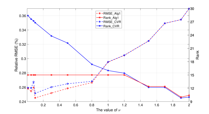
Figure 1: The average relative RMSE and rank of two solvers under different $\lambda$

5.2 Illustration of linear convergence

We take a matrix completion problem for example to illustrate the linear convergence of Algorithm 1 without accelerated strategy when solving problem (6) under the noisy and full sample setting, i.e., $f(X)=\frac{1}{2}\|X-M\|^{2}$ for $X\!\in\mathbb{R}^{n\times m}$, where $M=M^{*}+E$ is a noisy observation. The true $M^{*}\in\mathbb{R}^{n\times m}$ is generated in the same way as in Subsection 5.1, and the noise matrix $E$ is randomly generated by $E=\frac{0.1\|M^{*}\|}{\|B\|_{F}}B$, where every entry of $B$ obeys the standard normal distribution $N(0,1)$. We take $n=m=3000$ and $r^{*}=15$.

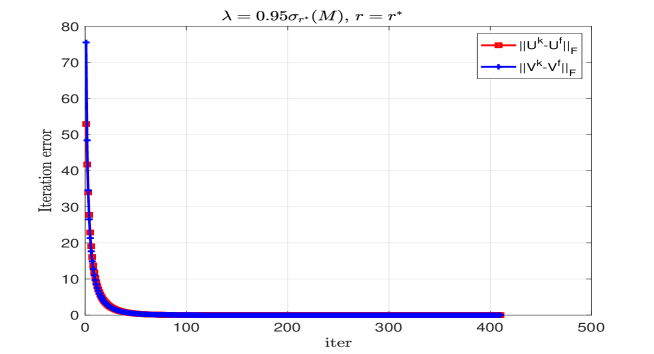
Figure 2: The iteration errors of Algorithm 1 for minimizing the function $\Phi_{\lambda}$

Figure 2 plots the iteration error curve $\|(U^{k},V^{k})-(U^{f},V^{f})\|_{F}$ of Algorithm 1, where $(U^{f},V^{f})$ is the final output of Algorithm 1 for solving (6) with $r=r^{*},\epsilon=10^{-10}$ and the number of max iteration $k_{\rm max}=5000$. We see that the sequence $\{(U^{k},V^{k})\}$ displays the linear convergence behavior. By the strict saddle property in [19], there is a high probability for the limit of $\{(U^{k},V^{k})\}$ to be a global optimal solution of problem (6) if $\lambda=0.95\sigma_{r^{*}}(M)$ is such that (5) has an optimal solution with rank at most $r^{*}$. Consequently, the convergence behavior is consistent with the result of Theorem 4.2.

6 Conclusion

For the factorization form (6) of the nuclear norm regularized problem, under a restricted condition number assumption on $\nabla^{2}f$, we have derived the error bound to the true $M^{*}$ for the non-strict critical points with rank at most $r^{*}$, which is demonstrated to be optimal in the ideal noiseless and full sampling setup. Furthermore, in the noisy and full sampling setup we have established the KL property of exponent $1/2$ of its objective function $\Phi_{\lambda}$ associated to almost all $\lambda>0$ in the global minimizer set, and in the noisy and partial sampling setup, have also achieved this property of $\Phi_{\lambda}$ only at a class of stationary points. This result, along with the strict saddle property in [19], partly improves the convergence analysis result of some first-order methods for problem (6) such as the alternating minimization methods in [25, 15]. It is interesting to consider the error bound of critical points for other equivalent or relaxed factorization form of the rank regularized model (2). We will leave them as our future research topics.

Acknowledgements. The authors are deeply indebted to Professor Bhojanapalli from Toyota Technological Institute at Chicago for providing some helpful comments on [2, Lemma 4.4]. The research of Shaohua Pan is supported by the National Natural Science Foundation of China under project No.11971177 and Guangdong Basic and Applied Basic Research Foundation (2020A1515010408).

Appendix A: The proof of Lemma 3.1.

Fix any critical point $(U,V)$ of $\Phi_{\lambda}$. Then, for any $(Z_{U},Z_{V})\in\mathbb{R}^{n\times r}\times\mathbb{R}^{m\times r}$, we have

$$\langle\nabla\Phi_{\lambda}(U,V),Z\rangle=0\ \ {\rm with}\ Z=(Z_{U};Z_{V}).$$

Recall that $M^{*}=U^{*}{V^{*}}^{\mathbb{T}}$ with $(U^{*},V^{*})\in\mathcal{E}^{*}$. From (14), this equality is equivalent to

$$\Big{\langle}\left(\begin{array}[]{cc}\textbf{ 0}&\nabla\!f(X)-\nabla\!f(M^{*})\\ \nabla\!f(X)^{\mathbb{T}}-\nabla\!f(M^{*})^{\mathbb{T}}&\textbf{0}\\ \end{array}\right),ZW^{\mathbb{T}}\Big{\rangle}+\langle\Xi(M^{*}),ZW^{\mathbb{T}}\rangle=0$$ (53)

$$\Longleftrightarrow\langle\nabla\!f(X)-\nabla\!f(M^{*}),Z_{U}V^{\mathbb{T}}+UZ_{V}^{\mathbb{T}}\rangle+\langle\Xi(M^{*}),ZW^{\mathbb{T}}\rangle=0$$

$$\Longleftrightarrow\int_{0}^{1}\nabla^{2}f(tX+(1-t)M^{*})(X-M^{*},Z_{U}V^{\mathbb{T}}+UZ_{V}^{\mathbb{T}})dt+\langle\Xi(M^{*}),ZW^{\mathbb{T}}\rangle=0$$ (54)

where $X=UV^{\mathbb{T}}$. Since ${\rm rank}([X\!-M^{*}\ \ Z_{U}V^{\mathbb{T}}+UZ_{V}^{\mathbb{T}}])\leq 4r^{*}$, by Lemma 2.1 we have

$$\Big{|}\frac{2}{\alpha+\beta}\nabla^{2}f(tX+(1-t)M^{*})(X\!-\!M^{*},Z_{U}V^{\mathbb{T}}+UZ_{V}^{\mathbb{T}})-\langle X\!-\!M^{*},Z_{U}V^{\mathbb{T}}+UZ_{V}^{\mathbb{T}}\rangle\Big{|}$$

$$\leq\frac{\beta-\alpha}{\alpha+\beta}\big{\|}UV^{\mathbb{T}}-U^{*}{V^{*}}^{\mathbb{T}}\big{\|}_{F}\big{\|}Z_{U}V^{\mathbb{T}}+UZ_{V}^{\mathbb{T}}\big{\|}_{F}.$$

By combining this inequality with equation (53), it follows that

$$\Big{|}\underbrace{\frac{2}{\alpha+\beta}\langle\Xi(M^{*}),ZW^{\mathbb{T}}\rangle}_{I_{1}}+\underbrace{\langle UV^{\mathbb{T}}-U^{*}(V^{*})^{\mathbb{T}},Z_{U}V^{\mathbb{T}}+UZ_{V}^{\mathbb{T}}\rangle}_{I_{2}}\Big{|}$$

$$\leq\frac{\beta-\alpha}{\alpha+\beta}\|UV^{\mathbb{T}}-U^{*}(V^{*})^{\mathbb{T}}\|_{F}\underbrace{\|Z_{U}V^{\mathbb{T}}+UZ_{V}^{\mathbb{T}}\|_{F}}_{I_{3}}.$$ (55)

Now take $Z=(WW^{\mathbb{T}}-W^{*}(W^{*})^{\mathbb{T}})(W^{\mathbb{T}})^{\dagger}$ where $W^{*}$ is defined as in (8) with $(U^{*},V^{*})$. Since the column orthonormal matrix $Q$ spans the subspace ${\rm col}(W)$, it is not hard to check that $(W^{\mathbb{T}})^{\dagger}W^{\mathbb{T}}=QQ^{\mathbb{T}}$. Then, it follows that $ZW^{\mathbb{T}}=(WW^{\mathbb{T}}-W^{*}(W^{*})^{\mathbb{T}})QQ^{\mathbb{T}}$. Next we bound the terms $I_{1},I_{2}$ and $I_{3}$ successively. First, for the term $I_{1}$, it holds that

$$I_{1}=\frac{2}{\alpha+\beta}\langle\Xi(M^{*}),ZW^{\mathbb{T}}\rangle=\frac{2}{\alpha+\beta}\langle\Xi(M^{*}),(WW^{\mathbb{T}}-W^{*}(W^{*})^{\mathbb{T}})QQ^{\mathbb{T}}\rangle.$$ (56)

For the term $I_{2}$, by recalling the definition of the linear operator $\mathcal{P}_{\rm off}$, we have

$$I_{2}=\langle UV^{\mathbb{T}}-U^{*}(V^{*})^{\mathbb{T}},Z_{U}V^{\mathbb{T}}+UZ_{V}^{\mathbb{T}}\rangle=\langle\mathcal{P}_{\rm off}(WW^{\mathbb{T}}-W^{*}(W^{*})^{\mathbb{T}}),ZW^{\mathbb{T}}\rangle.$$

By the expressions of $W,W^{*}$ and $\widehat{W},\widehat{W}^{*}$, it is not hard to check that

$$\mathcal{P}_{\rm off}(WW^{\mathbb{T}}-W^{*}(W^{*})^{\mathbb{T}})=\frac{1}{2}\big{[}WW^{\mathbb{T}}-W^{*}(W^{*})^{\mathbb{T}}-\widehat{W}\widehat{W}^{\mathbb{T}}+\widehat{W}^{*}(\widehat{W}^{*})^{\mathbb{T}}\big{]},$$

which along with $ZW^{\mathbb{T}}=(WW^{\mathbb{T}}-W^{*}(W^{*})^{\mathbb{T}})QQ^{\mathbb{T}}$ implies that

$$I_{2} =\frac{1}{2}\langle WW^{\mathbb{T}}-W^{*}(W^{*})^{\mathbb{T}},(WW^{\mathbb{T}}-W^{*}(W^{*})^{\mathbb{T}})QQ^{\mathbb{T}}\rangle$$

$$\quad-\frac{1}{2}\langle\widehat{W}\widehat{W}^{\mathbb{T}}-\widehat{W}^{*}(\widehat{W}^{*})^{\mathbb{T}},(WW^{\mathbb{T}}-W^{*}(W^{*})^{\mathbb{T}})QQ^{\mathbb{T}}\rangle.$$

Since $(U,V)$ is a stationary point of $\Phi_{\lambda}$, from Lemma 2.2 and $(U^{*},V^{*})\in\mathcal{E}^{*}$ we have

$$\langle\widehat{W}\widehat{W}^{\mathbb{T}}-\widehat{W}^{*}(\widehat{W}^{*})^{\mathbb{T}},(WW^{\mathbb{T}}-W^{*}(W^{*})^{\mathbb{T}})QQ^{\mathbb{T}}\rangle$$

$$=-\langle\widehat{W}\widehat{W}^{\mathbb{T}},W^{*}(W^{*})^{\mathbb{T}}QQ^{\mathbb{T}}\rangle-\langle\widehat{W}^{*}(\widehat{W}^{*})^{\mathbb{T}},WW^{\mathbb{T}}QQ^{\mathbb{T}}\rangle$$

$$=-\langle\widehat{W}^{*}(\widehat{W}^{*})^{\mathbb{T}},WW^{\mathbb{T}}\rangle\leq 0$$

where the second equality is using $QQ^{\mathbb{T}}=(W^{\mathbb{T}})^{\dagger}W^{\mathbb{T}}$, $\widehat{W}^{\mathbb{T}}W=0$ and $(\widehat{W}^{*})^{\mathbb{T}}W^{*}=0$, and the inequality is due to the positive semidefiniteness of $\widehat{W}^{*}(\widehat{W}^{*})^{\mathbb{T}}$ and $WW^{\mathbb{T}}$. Thus,

$$I_{2}\geq\frac{1}{2}\|(WW^{\mathbb{T}}-W^{*}(W^{*})^{\mathbb{T}})Q\|_{F}^{2}=\frac{1}{2}\|(WW^{\mathbb{T}}-W^{*}(W^{*})^{\mathbb{T}})QQ^{\mathbb{T}}\|_{F}^{2}.$$ (57)

For the term $I_{3}$, by recalling that $Z=(WW^{\mathbb{T}}-W^{*}(W^{*})^{\mathbb{T}})(W^{\mathbb{T}})^{\dagger}$, we calculate that

$$I_{3} =\|Z_{U}V^{\mathbb{T}}+UZ_{V}^{\mathbb{T}}\|_{F}\leq\sqrt{2}\|\mathcal{P}_{\rm off}(ZW^{\mathbb{T}})\|_{F}=\|ZW^{\mathbb{T}}\|_{F}$$

$$=\|(WW^{\mathbb{T}}-W^{*}(W^{*})^{\mathbb{T}})QQ^{\mathbb{T}}\|_{F}.$$ (58)

Now combining equation (56)-(Error bound of critical points and KL property of exponent $1/2$ for squared F-norm regularized factorization) with (Error bound of critical points and KL property of exponent $1/2$ for squared F-norm regularized factorization) yields the desired result. $\Box$

Appendix B: The proof of Lemma 3.2.

Since $\Delta\Delta^{\mathbb{T}}\!=\!WW^{\mathbb{T}}-W(W^{*}R_{1}^{*})^{\mathbb{T}}-W^{*}R_{1}^{*}W^{\mathbb{T}}+W^{*}(W^{*})^{\mathbb{T}}$ where $R_{1}^{*}$ is the matrix consisting of the first $r^{*}$ rows of $R^{*}$, with $X=UV^{\mathbb{T}}$ it follows that

$$2\langle\nabla\!f(X),\Delta_{U}\Delta_{V}^{\mathbb{T}}\rangle+\lambda\langle\Delta,\Delta\rangle=\langle\Xi(X),\Delta\Delta^{\mathbb{T}}\rangle$$

$$=\big{\langle}\Xi(X),WW^{\mathbb{T}}-W(W^{*}R_{1}^{*})^{\mathbb{T}}-W^{*}R_{1}^{*}W^{\mathbb{T}}+W^{*}(W^{*})^{\mathbb{T}}\big{\rangle}$$

$$=\big{\langle}\Xi(X),W^{*}(W^{*})^{\mathbb{T}}\big{\rangle}=\big{\langle}\Xi(X),W^{*}(W^{*})^{\mathbb{T}}-WW^{\mathbb{T}}\big{\rangle}$$

where the third equality is due to $\Xi(X)W=0$ and $\Xi(X)=\Xi(X)^{\mathbb{T}}$. Together with (2.2), we get (3.2). We next show that (23) holds. From $\nabla^{2}\Phi_{\lambda}(U,V)(\Delta,\Delta)\geq 0$ and (3.2),

$$\nabla^{2}f(X)(U\Delta_{V}^{\mathbb{T}}+\Delta_{U}V^{\mathbb{T}},U\Delta_{V}^{\mathbb{T}}+\Delta_{U}V^{\mathbb{T}})\geq\langle\Xi(X),WW^{\mathbb{T}}-W^{*}(W^{*})^{\mathbb{T}}\rangle.$$ (59)

According to the given assumption on $f$, it is immediate to have that

$$\nabla^{2}f(X)(U\Delta_{V}^{\mathbb{T}}+\Delta_{U}V^{\mathbb{T}},U\Delta_{V}^{\mathbb{T}}+\Delta_{U}V^{\mathbb{T}}) \leq\beta\|U\Delta_{V}^{\mathbb{T}}+\Delta_{U}V^{\mathbb{T}}\|_{F}^{2},$$

$$\leq 2\beta(\|U\Delta_{V}^{\mathbb{T}}\|^{2}_{F}+\|\Delta_{U}V^{\mathbb{T}}\|_{F}^{2}).$$ (60)

In addition, from the restricted strong convexity of $f$, it follows that

$$\langle\Xi(X),WW^{\mathbb{T}}-W^{*}(W^{*})^{\mathbb{T}}\rangle$$

$$=\langle\Xi(X)-\Xi(M^{*}),WW^{\mathbb{T}}-W^{*}(W^{*})^{\mathbb{T}}\rangle+\langle\Xi(M^{*}),WW^{\mathbb{T}}\!-\!W^{*}(W^{*})^{\mathbb{T}}\rangle$$

$$=2\langle\nabla f(X)\!-\!\nabla f(M^{*}),X\!-\!M^{*}\rangle+\langle\Xi(M^{*}),WW^{\mathbb{T}}\!-\!W^{*}(W^{*})^{\mathbb{T}}\rangle$$

$$=2\int_{0}^{1}\nabla^{2}\!f(M^{*}+t(X\!-\!M^{*}))(X\!-\!M^{*},X\!-\!M^{*})dt+\langle\Xi(M^{*}),WW^{\mathbb{T}}-W^{*}(W^{*})^{\mathbb{T}}\rangle$$

$$\geq 2\alpha\|X-M^{*}\|_{F}^{2}+\langle\Xi(M^{*}),WW^{\mathbb{T}}\!-\!W^{*}(W^{*})^{\mathbb{T}}\rangle.$$

Together with inequalities (59) and (Error bound of critical points and KL property of exponent $1/2$ for squared F-norm regularized factorization), we obtain

$$2\beta(\|U\Delta_{V}^{\mathbb{T}}\|^{2}_{F}+\|\Delta_{U}V^{\mathbb{T}}\|_{F}^{2})\geq 2\alpha\|X-M^{*}\|_{F}^{2}+\langle\Xi(M^{*}),WW^{\mathbb{T}}-W^{*}(W^{*})^{\mathbb{T}}\rangle$$

$$\Longleftrightarrow\beta\|W\Delta^{\mathbb{T}}\|_{F}^{2}\geq 2\alpha\|X-M^{*}\|_{F}^{2}+\langle\Xi(M^{*}),WW^{\mathbb{T}}-W^{*}(W^{*})^{\mathbb{T}}\rangle$$ (61)

where the equivalence is due to $\|U\Delta_{V}^{\mathbb{T}}\|^{2}_{F}=\|V\Delta_{V}^{\mathbb{T}}\|_{F}^{2}$ and $\|V\Delta_{U}^{\mathbb{T}}\|^{2}_{F}=\|U\Delta_{U}^{\mathbb{T}}\|_{F}^{2}$, implied by $U^{\mathbb{T}}U=V^{\mathbb{T}}V$. From [19, Lemma 4.5] it follows that

$$\|WW^{\mathbb{T}}-W^{*}(W^{*})^{\mathbb{T}}\|^{2}_{F} =\|\mathcal{P}_{\rm on}(WW^{\mathbb{T}}-W^{*}(W^{*})^{\mathbb{T}})\|^{2}_{F}+\|\mathcal{P}_{\rm off}(WW^{\mathbb{T}}-W^{*}(W^{*})^{\mathbb{T}})\|^{2}_{F}$$

$$\leq 2\|\mathcal{P}_{\rm off}(WW^{\mathbb{T}}-W^{*}(W^{*})^{\mathbb{T}})\|^{2}_{F}=4\|X-M^{*}\|_{F}^{2},$$

which implies that $2\alpha\|X-M^{*}\|_{F}^{2}\geq\frac{\alpha}{2}\|WW^{\mathbb{T}}-W^{*}(W^{*})^{\mathbb{T}}\|^{2}_{F}$. Together with (Error bound of critical points and KL property of exponent $1/2$ for squared F-norm regularized factorization), we obtain the desired inequality (23). The proof is completed. $\Box$

Appendix C:

The following lemma states the relation between the optimal solution set of (5) and the global optimal solution set of (6), whose proof is easy by the following result in [27]:

$$\|X\|_{*}=\min_{R\in\mathbb{R}^{n\times r},L\in\mathbb{R}^{m\times r}}\Big{\{}\frac{1}{2}\big{(}\|R\|_{F}^{2}+\|L\|_{F}^{2}\big{)}\ \ {\rm s.t.}\ \ X=RL^{\mathbb{T}}\Big{\}}.$$ (62)

Lemma 1

Fix any $\lambda>0$. If $(\overline{U},\overline{V})$ is globally optimal to problem (6), then $\overline{X}=\overline{U}{\overline{V}}^{\mathbb{T}}$ is an optimal solution of (5) over the set $\{X\in\mathbb{R}^{n\times m}\ |\ {\rm rank}(X)\leq r\}$; and conversely, if $\overline{X}$ is an optimal solution of (5) with ${\rm rank}(\overline{X})\leq r$, then $(\overline{R},\overline{L})$ with $\overline{R}=\overline{P}[{\rm Diag}(\sigma^{r}(\overline{X}))]^{1/2}$ and $\overline{L}=\overline{Q}[{\rm Diag}(\sigma^{r}(\overline{X}))]^{1/2}$ for $(\overline{P},\overline{Q})\in\mathbb{O}^{n,m}(\overline{X})$ is a global optimal solution to (6).

References

- [1] H. Attouch, J. Bolte, P. Redont and A. Soubeyran, Proximal alternating minimization and projection methods for nonconvex problems: an approach based on the Kurdyka-Łojasiewicz inequality, Mathematics of Operations Research, 35(2010): 438-457.
- [2] S. Bhojanapalli, B. Neyshabur and N. srebro, Global optimality of local search for low rank matrix recovery, Advances in Neural Information Processing Systems, 29(2016): 3873-3881.
- [3] S. Burer and R. D. Monteiro, A nonlinear programming algorithm for solving semidefinite programs with low-rank factorization, Mathematical Programming, 95(2003): 329-357.
- [4] Y. X. Chen, Y. J. Chi, J. Q. Fang, C. Ma and Y. L. Yan, Noisy matrix completion: understanding statistical guarantees for convex relaxation via nonconvex optimization, SIAM Journal on Optimization, 30(2020): 3098-3121.
- [5] T. T. Cai, C. H. Zhang and H. H. Zhou, Optimal rates of convergence for covariance matrix estimation, The Annals of Statistics, 38(2010): 2118-2144.
- [6] E. J. Candès and B. Recht, Exact matrix completion via convex optimization, Foundations of Computational Mathematics, 9(2009): 717-772.
- [7] E. J. Candès and Y. Plain, Tight oracle inequalities for low-rank matrix recovery from a minimal number of noisy random measurements, IEEE Transactions on Information Theory, 57(2011): 2342-2359.
- [8] J. Chi, R. Ge, P. Netrapalli, S. M. Kakade and M. I. Jordan, How to escape saddle points efficiently, Proceedings of the 34th International Conference on Machine Learning, 70(2017): 1724-1732.
- [9] A. Datta and H. Zou, CoCoLASSO for high-dimensional error-in-variables regression, The Annals of Statistics, 45(2017): 2400-2426.
- [10] M. A. Davenport and J. Romberg, An overview of low-rank matrix recovery from incomplete observations, IEEE Journal of Selected Topics in Signal Processing, 10(2016): 608-622.
- [11] M. Fazel, Matrix rank minimization with applications, PhD thesis, Stanford University, 2002.
- [12] R. Ge, F. Huang, C. Jin and Y. Yuan, Escaping from saddle points—online stochastic gradient for tensor decomposition, Proceedings of the 28th Conference on Learning Theory, 40(2015): 797-842.
- [13] R. Ge, C. Jin and Y. Zheng, No spurious local minima in nonconvex low rank problems: A unified geometric analysis, Proceedings of the 34th International Conference on Machine Learning, 70(2017): 1233-1242.
- [14] D. Gross, Y. K. Liu, S. T. Flammia, S. Becker and J. Eisert, Quantum state tomography via compressed sensing, Physical Review Letters, 105(2010): 1-4.
- [15] T. Hastie, R. Mazumder, J. D. Lee and R. Zadeh, Matrix completion and low-rank SVD via fast alternating least squares, Journal of Machine Learning Research 16(2015): 3367-3402.
- [16] P. Jain, P. Netrapalli and S. Sanghavi, Low-rank matrix completion using alternating minimization, In Proceedings of the 45th annual ACM Symposium on Theory of Computing, 2013: 665-674.
- [17] J. D. Lee, I. Panageas, G. Piliouras, M. Simchowitz, M. I. Jordan and B. Recht, First-order methods almost always avoid strict saddle points, Mathematical Programming, 176(2019): 311-337.
- [18] X. G. Li, J. W. Lu, R. Arora, J. Haupt, H. Liu, Z. R. Wang and T. Zhao, Symmetry, saddle points, and global optimization landscape of nonconvex matrix factorization, IEEE Transactions on Information Theory, 65(2019): 3489-3514.
- [19] Q. W. Li, Z. H. Zhu and G. G. Tang, The non-convex geometry of low-rank matrix optimization, Information and Inference: A Journal of the IMA, 8(2018): 51-96.
- [20] S. Negahban and M. J. Wainwright, Estimation of (near) low-rank matrices with noise and high-dimensional scaling, The Annals of Statistics, 39(2011): 1069-1097.
- [21] S. Negahban and M. J. Wainwright, Restricted strong convexity and weighted matrix completion: Optimal bounds with noise, Journal of Machine Learning Research, 13(2012): 1665-1697.
- [22] Y. Nesterov, A method of solving a convex programming problem with convergence rate , Soviet Mathematics Doklady, 27(1983): 372-376.
- [23] D. Park, A. Kyrillidis, C. Caramanis and S. Sanghavi, Finding low-rank solution via non-convex matrix factorization efficiently and provably, SIAM Journal on Imaging Sciences, 11(2018): 2165-2204.
- [24] D. Park, A. Kyrillidis, C. Caramanis and S. Sanghavi, Non-square matrix sensing without spurious local minima via the Burer-Monteiro approach, In Proceedings of the 20th International Conference on Artificial Intelligence and Statistics, 54(2017): 65-74.
- [25] B. Recht, M. Fazel and P. A. Parrilo, Guaranteed minimum-rank solutions of linear matrix equations via nuclear norm minimization, SIAM Review, 52(2010): 471-501.
- [26] R. T. Rockafellar and R. J-B. Wets, Variational analysis, Springer, 1998.
- [27] J. D. M. Rennie and N. Srebro, Fast maximum margin matrix factorization for collaborative prediction, In Proceedings of the 22nd International Conference on Machine Learning, 2005: 713-719.
- [28] A. Saumard and J. A. Wellner, Log-concavity and strong log-concavity: a review, Statistics Surveys, 8(2014): 45-114.
- [29] J. Sun, When are nonconvex optimization problems not scary? PhD thesis, Columbia University, 2016.
- [30] R. Y. Sun and Z. Q. Luo, Guaranteed matrix completion via non-convex factorization, IEEE Transactions on Information Theory, 62(2016): 6535-6579.
- [31] K. C. Toh and S. W. Yun, An accelerated proximal gradient algorithm for nuclear norm regularized least squares problems, Pacific Journal of Optimization, 6(2010): 615-640.
- [32] S. Tu, R. Boczar, M. Simchowitz, M. Soltanolkotabi and B. Recht, Low-rank solution of linear matrix equations via procrustes flow, In International Conference on Machine Learning, 48(2016): 964-973.
- [33] R. Vershynin, Introduction to the Non-asymptotic Analysis of Random Matrices. Compressed Sensing: Theory and Applications, Cambridge University Press, 2012: 210-268.
- [34] Y. Y. Xu and W. T. Yin, A block coordinate descent method for regularized multiconvex optimization with applications to nonnegative tensor factorization and completion, SIAM Journal on Image Science, 6(2013): 1758-1789.
- [35] X. Zhang, L. X. Wang, Y. D. Yu and Q. Q. Gu, A primal-dual analysis of global optimality in nonconvex low-rank matrix recovery, In International conference on machine learning, 80(2018): 5862-5871.
- [36] Q. Zhang, C. H. Chen, H. K. Liu and A. M. C. So, On the linear convergence of the ADMM for regularized non-convex low-rank matrix recovery, https://www1.se.cuhk.edu.hk/~manchoso/admm_MF.pdf, 2018.
- [37] T. Zhao, Z. Wang and H. Liu, A nonconvex optimization framework for low rank matrix estimation, Advances in Neural Information Processing Systems, 1(2015): 559-567.
- [38] Q. Zheng and J. Lafferty, A convergent gradient descent algorithm for rank minimization and semidefinite programming from random linear measurements, Advances in Neural Information Processing Systems, 1(2015): 109-117.
- [39] Z. H. Zhu, Q. W. Li, G. G. Tang and M. B. Wakin, Global optimization in low-rank matrix optimization, IEEE Transactions on Signal Processing, 66(2018): 3614-3628.
- [40] Z. H. Zhu, Q. W. Li, G. G. Tang and M. B. Wakin, The global optimization geometry in low-rank matrix optimization, IEEE Transactions on Information Theory, 67(2021): 1308-1331.