MAP Clustering under the Gaussian Mixture Model via
Mixed Integer Nonlinear Optimization

Abstract

We present a global optimization approach for solving the maximum a-posteriori (MAP) clustering problem under the Gaussian mixture model. Our approach can accommodate side constraints and it preserves the combinatorial structure of the MAP clustering problem by formulating it as a mixed-integer nonlinear optimization problem (MINLP). We approximate the MINLP through a mixed-integer quadratic program (MIQP) transformation that improves computational aspects while guaranteeing $\epsilon$-global optimality. An important benefit of our approach is the explicit quantification of the degree of suboptimality, via the optimality gap, en route to finding the globally optimal MAP clustering. Numerical experiments comparing our method to other approaches show that our method finds a better solution than standard clustering methods. Finally, we cluster a real breast cancer gene expression data set incorporating intrinsic subtype information; the induced constraints substantially improve the computational performance and produce more coherent and biologically meaningful clusters.

1 Introduction

In the application of clustering models to real data there is often rich prior information that constrains the relationships among the samples, or the relationships between the samples and the parameters. For example, in biological or clinical experiments, it may be known that two samples are technical replicates and should be assigned to the same cluster, or it may be known that the mean value for control samples is in a certain range. However, standard model-based clustering methods make it difficult to enforce such hard logical constraints and may fail to provide a globally optimal clustering.

Locally optimal and heuristic clustering methods lack optimality guarantees or bounds on solution quality that indicate the potential for further improvement. Even research on bounding the quality of heuristic solutions is scarce (Cochran,, 2018). Conversely, a rigorous optimization framework affords bounds that establish the degree of suboptimality for any feasible solution, and a certificate of global optimality thereby guaranteeing that no better clustering exists.

Recent work on developing global optimization methods for supervised learning problems has led to impressive improvements in the size of the problems that can be handled. In linear regression, properties such as stability to outliers and robustness to predictor uncertainty have been represented as a mixed-integer quadratic program and solved for samples of size $n\sim 1,000$ (Bertsimas and King,, 2016; Bertsimas and Li,, 2020). Best subset selection in the context of regression is typically approximated as a convex problem with the $\ell_{1}$ norm penalty, but can now be solved exactly using the nonconvex $\ell_{0}$ penalty for thousands of data points (Bertsimas et al.,, 2016). In unsupervised learning, Bandi et al., (2019) use mixed-integer optimization (MIO) to learn parameters for the Gaussian mixture model, showing that an optimization-based approach can outperform the EM algorithm. Greenberg et al., (2019) use a trellis representation and dynamic programming to compute the partiton function exactly and thus the probability of all possible clusterings. For these reasons we are motivated to develop a method for achieving a globally optimal solution for clustering under the Gaussian mixture model that allows for the incorporation of rich prior constraints.

Finite mixture model

The probability density function of a finite mixture model is $p(\bm{y}|\bm{\theta},\bm{\pi})=\sum_{k=1}^{K}\pi_{k}p(\bm{y}|\bm{\theta}_{k})$ where the observed data is $\bm{y}$ and the parameter set is $\bm{\phi}=\{\bm{\theta},\bm{\pi}\}$. The data is an $n\text{-tuple}$ of $d\text{-dimensional}$ random vectors $\bm{y}=(\bm{y}_{1}^{T},\ldots,\bm{y}_{n}^{T})^{T}$ and the mixing proportion parameter $\bm{\pi}=(\pi_{1},\ldots,\pi_{K})^{T}$ is constrained to the probability simplex $\mathcal{P}_{K}=\Set{\bm{p}\in\mathbb{R}^{K}}{\bm{p}\succeq 0\ \textrm{and}\ \mathbf{1}^{T}\bm{p}=1}$. When the component density, $p(\bm{y}|\bm{\theta}_{k})$, is a Gaussian density function, $p(\bm{y}|\bm{\phi})$ is a Gaussian mixture model with parameters $\bm{\theta}=\left(\{\bm{\mu}_{1},\bm{\Sigma}_{1}\},\ldots,\{\bm{\mu}_{K},\bm{\Sigma}_{K}\}\right)$. Assuming independent, identically distributed (iid) samples, the Gaussian mixture model probability density function is $p(\bm{y}|\bm{\theta},\bm{\pi})=\prod_{i=1}^{n}\sum_{k=1}^{K}\pi_{k}\ p\left(\bm{y}_{i}|\bm{\mu}_{k},\bm{\Sigma}_{k}\right)$.

Generative model

A generative model for the Gaussian mixture density function is

$$\begin{split}Z_{i}&\overset{\text{iid}}{\sim}\textrm{Categorical}(\bm{\pi})\quad\text{for}\ i=1,\ldots,n,\\ Y_{i}|z_{i},\bm{\theta}&\sim\textrm{Gaussian}(\bm{\mu}_{z_{i}},\bm{\Sigma}_{z_{i}}),\end{split}$$ (1)

where $\bm{\mu}=(\bm{\mu}_{1},\ldots,\bm{\mu}_{K})$ and $\bm{\Sigma}=(\bm{\Sigma}_{1},\ldots,\bm{\Sigma}_{K})$. To generate data from the Gaussian mixture model, first draw $z_{i}\in\{1,\ldots,K\}$ from a categorical distribution with parameter $\bm{\pi}$. Then, given $z_{i}$, draw $\bm{y}_{i}$ from the associated Gaussian component distribution $p(\bm{y}_{i}|\bm{\theta}_{z_{i}})$.

Maximum a posteriori (MAP) clustering

The posterior distribution function for the generative Gaussian mixture model is

$$p(\bm{z},\bm{\theta},\bm{\pi}|\bm{y})=\frac{p(\bm{y}|\bm{\theta},\bm{z})p(\bm{z}|\bm{\pi})p(\bm{\theta},\bm{\pi})}{p(\bm{y})}.$$ (2)

The posterior distribution requires the specification of a prior distribution $p(\bm{\theta},\bm{\pi})$, and if $p(\bm{\theta},\bm{\pi})\propto 1$, then MAP clustering is equivalent to maximum likelihood clustering. The MAP estimate for the component membership configuration can be obtained by solving the following optimization problem:

z, θ, π logp(z, θ, π | y) z_i∈{1, …, K}   ∀i π∈P_K.

Assuming iid sampling, the objective function comprises the following conditional density functions:

$$p(\bm{y}_{i}|\bm{\mu},\bm{\Sigma},\bm{z}_{i}) =\prod_{k=1}^{K}\left[(2\pi)^{-m/2}|\bm{\Sigma}_{k}|^{-1/2}\right.$$

$$\left.\quad\cdot\exp\left(-\frac{1}{2}(\bm{y}_{i}-\bm{\mu}_{k})^{T}\bm{\Sigma}^{-1}_{k}(\bm{y}_{i}-\bm{\mu}_{k})\right)\right]^{z_{ik}},$$

$$p(\bm{z}_{i}|\bm{\pi}) =\prod_{k=1}^{K}\left[\pi_{k}\right]^{z_{ik}},\qquad p(\bm{\Sigma},\bm{\pi},\bm{\mu})\propto 1,$$

where $z_{i}\in\{1,\ldots,K\}$ is recast using binary encoding. To simplify the presentation, consider the case of one-dimensional data ($d=1$) and equivariant components ($\bm{\Sigma}_{1}=\cdots=\bm{\Sigma}_{K}=\sigma^{2}$). The MAP optimization problem can be written |s| z, μ, π η∑_i=1^n ∑_k=1^K z_ik (y_i - μ_k)^2 - ∑_i=1^n ∑_k=1^K z_ik logπ_k ∑_k=1^K π_k=1 ∑_k=1^K z_ik=1, i=1,…,n M_k^L ≤μ_k≤M_k^U, k=1,…,K π_k≥0, k=1,…,K z_ik∈{0,1}, i=1, …, n k=1, …, K,

where $\eta=\frac{1}{2\sigma^{2}}$ is the precision, and $M_{k}^{L}$ and $M_{k}^{U}$ are real numbers. In a fully Bayesian setting, even if the MAP clustering is of less interest than the full distribution function, the MAP clustering can still be useful as an initial value for a posterior sampling algorithm as suggested by Gelman and Rubin, (1996).

Biconvex mixed-integer nonlinear programming

While maximum a posterior clustering for a Gaussian mixture model is a well-known problem, it does not fall neatly into any optimization problem formulation except the broadest class: mixed-integer nonlinear programming. Here we show that, in fact, maximum a posteriori clustering for the Gaussian mixture model is in a more restricted class of optimization problems—biconvex mixed-integer nonlinear problems. This fact can be exploited to develop improved inference algorithms.

Theorem 1.

Maximum a posteriori clustering under the Gaussian mixture model (1) with known covariance is a biconvex mixed-integer nonlinear programming optimization problem.

Proof.

We briefly sketch a proof that is provided in full in the Supplementary Material. A biconvex mixed-integer nonlinear program (MINLP) is an optimization problem such that if the integer variables are relaxed, the resulting optimization problem is a biconvex nonlinear programming problem. Maximum a posteriori clustering under Model (1) can be written as Problem (1). If $z_{ik}\in\{0,1\}$ is relaxed to $z_{ik}\in[0,1]$, Problem (1) is convex in $\{\bm{\pi},\bm{\mu}\}$ for fixed $\bm{z}$ and convex in $\bm{z}$ for fixed $\{\bm{\pi},\bm{\mu}\}$, and it satisfies the criteria of a biconvex nonlinear programming optimization problem (Floudas,, 2000). Because the relaxed problem is a biconvex nonlinear program, the original maximum a posteriori clustering problem is a biconvex MINLP. ∎

Goal of this work

Our goal is to solve for the global MAP clustering via a MINLP over the true posterior distribution domain while only imposing constraints that are informed by our prior knowledge and making controllable approximations. Importantly, there are no constraints linking $\bm{\pi}$, $\bm{\mu}$, and $\bm{z}$ such as $\pi_{k}=\frac{1}{n}\sum_{i=1}^{n}z_{ik},\ k=1,\ldots,K$ which would be a particular estimator.

Computational complexity

Problems in the MINLP class are NP-hard in general, and the MAP problem in particular presents two primary computational challenges (Murty and Kabadi,, 1987). First, as the number of data points increases, the size of the configuration space of $\bm{z}$ increases in a combinatorial manner (Nemhauser and Wolsey,, 1988). Second, the nonlinear objective function can have many local minima. Despite these worst-case complexity results, MINLP problems are increasingly often solved to global optimality in practice. Good empirical performance is often due to exploiting problem-specific structures and powerful algorithmic improvements such as branch-and-bound, branch-and-cut, and branch-and-reduce algorithms (Bodic and Nemhauser,, 2015; Tawarmalani and Sahinidis,, 2005).

Contributions of this work

This work has three main contributions:

• We provide an exact formulation to find globally optimal solutions to the MAP clustering problem and demonstrate that it is tractable for instances formed from small data sets, as well as for larger instances when incorporating side constraints.

• We reformulate the original MINLP by using a piecewise approximation to the objective entropy term and a constraint-based formulation of the mixed-integer-quadratic objective term, thus converting the problem to a mixed-integer quadratic program (MIQP), and show that it achieves approximately two orders of magnitude improvement in computation time over the MINLP for larger data set size instances.

• We apply our approach to a real breast cancer data set and show that our MIQP method results in intrinsic subtype assignments that are more biologically consistent than the standard method for subtype assignment.

Section 2 describes related work and summarizes the relationship between some existing clustering procedures and the MINLP formulation. Section 3 describes our MIQP formulation and a branch-and-bound algorithm. Section 4 reports the results of comparisons between our methods and standard clustering procedures. Section 5 presents a discussion of the results and future work.

2 Related Work

Many MAP clustering methods can be interpreted as a specific combination of a relaxation of Problem (1) and a search algorithm for finding a local or global minimum. Table 1 summarizes these relationships.

Table 1: Summary of approximation methods for MAP clustering in an optimization framework.

Method	Domain Relaxation	Objective Approximation	Search Algorithm
EM Algorithm	$\checkmark$	–	coordinate/stochastic descent
Variational EM	$\checkmark$	$\checkmark$	coordinate/stochastic descent
SLSQP	$\checkmark$	$\checkmark$	coordinate descent
Simulated Annealing	$\checkmark$	–	stochastic descent
Learning Parameters via MIO	$\checkmark$	$\checkmark$	coordinate descent

EM algorithm

The EM algorithm relaxes the domain such that $z_{ik}\in[0,1]$ instead of $z_{ik}\in\{0,1\}$. The decision variables of the resulting biconvex optimization problem are partitioned into two groups: $\{\bm{z}\}$ and $\{\bm{\mu},\bm{\pi}\}$. The search algorithm performs coordinate ascent on these two groups. There are no guarantees for the global optimality of the estimate produced by the EM algorithm. While Balakrishnan et al., (2017) showed that the global optima of a mixture of well-separated Gaussians may have a relatively large region of attraction, Jin et al., (2016) showed that inferior local optima can be arbitrarily worse than the global optimum.

Variational EM

The variational EM algorithm introduces a surrogate function $q(\bm{z},\phi|\bm{\xi})$ for the posterior distribution $p(\bm{z},\bm{\phi}|\bm{y})$ (Beal and Ghahramani,, 2003). First, the surrogate is fit to the posterior by solving $\hat{\bm{\xi}}\in\arg\min_{\bm{\xi}}\ \textrm{KL}(q(\phi,\bm{z}|\xi)\ ||\ p(\phi,\bm{z}|\bm{y}))$. Then the surrogate is used in place of the posterior distribution in the original optimization problem $\hat{\phi},\hat{\bm{z}}\in\arg\min_{\phi,\bm{z}}\ \log q(\theta,\bm{z}|\bm{\xi})$. The search algorithm performs coordinate ascent on $\{\phi,\bm{z}\}$ and $\bm{\xi}$. The computational complexity is improved over the original MAP problem by selecting a surrogate that has favorable structure (linear or convex) and by relaxing the domain of the optimization problem. This surrogate function approach has existed in many fields; it is alternatively known as majorization-minimization (Lange et al.,, 2000) and has deep connections with Franke-Wolfe gradient methods and block coordinate descent methods (Mairal,, 2013). The domain of the problem can be viewed as a marginal polytope and outer approximations of the marginal polytope lead to efficient sequential approximation methods that have satisfying theoretical properties (Wainwright and Jordan,, 2007).

SLSQP

Sequential Least-Squares Quadratic Programming (SLSQP) is a popular general-purpose constrained nonlinear optimization method that uses a quadratic surrogate function to approximate the Lagrangian (Nocedal and Wright,, 2006). In SLSQP, the surrogate function is a quadratic approximation of the Lagrangian of the original problem. The domain of the original problem is also relaxed so that the constraint cuts it generates are approximated by linear functions. Like variational EM, SLSQP iterates between fitting the surrogate function and optimizing over the decision variables. Quadratic surrogate functions have also been investigated in the context of variational EM for nonconjugate models (Braun and McAuliffe,, 2010; Wang and Blei,, 2013).

Simulated annealing

Simulated annealing methods are theoretically guaranteed to converge to a global optimum of a nonlinear objective. However, choosing the annealing schedule for a particular problem is challenging and the guarantee of global optimality only exists in the limit of the number of steps; there is no general way to choose the annealing schedule or monitor convergence (Andrieu et al.,, 2003). Furthermore, designing a sampler for the binary $\bm{z}$ can be challenging unless the domain is relaxed. Even so, modern simulated annealing-type methods such a basin hopping have shown promise in practical applications (Wales and Doye,, 1997).

Branch-and-bound

In many practical optimization problems featuring combinatorial structure, it is critical to obtain the global optimum with a certificate of optimality, that is, with a (computational) proof that no better solution exists. For these situations, branch-and-bound methods, first proposed by Land and Doig, (1960), have seen the most success. While MINLP problems remain NP-hard in general, the scale of problems that can be solved to global optimality has increased dramatically in the past 20 years (Bertsimas and King,, 2017). The current state-of-the-art solver for general MINLPs is the Branch-and-Reduce Optimization Navigator (BARON). BARON exploits general problem structure to branch-and-bound with domain reduction on both discrete and continuous decision variables (Sahinidis,, 2017).

Learning parameters via MIO

Bandi et al., (2019) recently described a mixed-integer optimization formulation of the parameter estimation problem for the Gaussian mixture model. Conditional on the parameter estimates, they computed the one-sample-at-a-time MAP assignments for out-of-sample data. They convincingly demonstrate that a mixed-integer optimization approach can outperform the EM algorithm in terms of out-of-sample accuracy for real-world data sets.

Bandi et al., (2019) and our paper solve related, yet different problems. Their primary objective is density estimation—to find the optimal parameters of the Gaussian mixture model. Our primary objective is MAP clustering—to find an optimal maximum a posteriori assignment of data points to clusters and associated distribution parameters. To assign data points to clusters, Bandi et al., (2019) first estimates the model parameters and then computes the maximum a posteriori assignments conditioned on the estimated model parameters. Even so, Bandi et al., (2019) showed that an optimization framework can yield real benefits for learning problems.

3 Branch-and-Bound for MAP Clustering

Branch-and-bound solves the original problem with integer variables by solving a sequence of relaxations that partition the search space. The branch-and-bound algorithm provides for the opportunity to exclude large portions of the search space at each iteration, and if the branching strategy is well-suited to the problem it can substantially reduce the actual computation time for real problems (Grötschel,, 2012).

Our innovations to the standard MINLP fall into three categories: changes to the domain, changes to the objective function, and changes to the branch-and-bound algorithm. For the domain constraints, we formulate a symmetry-breaking constraint, specific estimators for $\bm{\pi}$ and $\bm{\mu}$, tightened parameter bounds, and logical constraints. For the objective function, we formulate the prior distribution $p(\bm{\pi},\bm{\mu})$ as a regularizer, a piecewise linear approximation to the nonlinear logarithm function, and an exact mapping of a mixed-integer quadratic term as a set of constraints.

A common difficulty in obtaining a global optimum for Problem (1) is that the optimal value of the objective is invariant to permutations of the component ordering. In the MINLP framework, we eliminate such permutations from the feasible domain by adding a simple linear constraint $\pi_{1}\leq\pi_{2}\leq\cdots\leq\pi_{K}.$ This set of constraints enforces an ordering, thereby reducing the search base and improving computational performance.

Though Problem 1 does not specify any particular form for the estimators of $\bm{\pi}$ or $\bm{\mu}$, it may be of interest to specify the estimators with equality constraints. For example the standard estimators of the EM algorithm are:

$$\pi_{k}=\frac{1}{n}\sum_{i=1}^{n}z_{ik},\quad\text{and}\quad\bm{\mu}_{k}=\frac{\sum_{i=1}^{n}\bm{y}_{i}z_{ik}}{\sum_{i=1}^{n}z_{ik}}\;\forall k.$$

The resulting optimization problem can be written entirely in terms of integer variables and the goal is to find the optimal configuration of $\bm{z}$. Note that Problem (1) does not specify these constraints and we do not enforce these particular estimators in our experiments in Section 4.

A conservative bound on $\bm{\mu}_{k}$ is $[\min(\bm{y}),\max(\bm{y})]$ and this bound is made explicit in Problem (1). Of course, prior information may be available that informs and reduces the range of these bounds. Placing more informative box constraints on the parameter values has been shown by Bertsimas et al., (2016) to greatly improve the computational time of similar MINLPs.

An important aspect of using the MINLP formulation as a Bayesian procedure is the ability to formulate logical constraints that encode rich prior information. These constraints shape the prior distribution domain in a way that is often difficult to express with standard probability distributions. Problem (1) already has one either/or logical constraint specifying that a data point $i$ must belong to exactly one component $k$. One can specify that data point $i$ and $j$ must be assigned to the same component, $z_{ik}=z_{jk},\ \forall k$ or that they must be assigned to different components, $z_{ik}+z_{jk}\leq 1,\ \forall k$. A non-symmetric constraint can specify that if data point $j$ is assigned to component $k$, then $i$ must be assigned to $k$, $z_{jk}\leq z_{ik}$; on the other hand, if $i$ is not assigned to component $k$, then $j$ cannot be assigned to component $k$. A useful constraint in the context of the GMM is the requirement that each component has a minimum number of data points assigned to it, $\sum_{i=1}^{n}z_{ik}\geq L,\quad\text{for}\ k=1,\ldots,K$, where $L$ is a specified number of data points. Additional logical constraints can be formulated in a natural way in the MINLP such as: packing constraints (from a set of data points $\mathcal{I}$, select at most $L$ to be assigned to component $k$), $\sum_{i\in\mathcal{I}}z_{ik}\leq L$; partitioning constraints (from a set of data points, select exactly $L$ to be assigned to component $k$) $\sum_{i\in\mathcal{I}}z_{ik}=L$; and covering constraints (from a set of data points select at least $L$) $\sum_{i\in\mathcal{I}}z_{ik}\geq L$.

3.1 Approximation via MIQP

Recall the objective function of Problem (1) is:

$$f(\bm{z},\bm{\pi},\bm{\mu};\bm{y},\eta)=\eta\sum_{k=1}^{K}\sum_{i=1}^{n}z_{ik}(\bm{y}_{i}-\mu_{k})^{2}-\sum_{i=1}^{n}\sum_{k=1}^{K}z_{ik}\log\pi_{k}.$$

The objective function is mixed-integer and nonlinear due to the product of $z_{ik}$ and $\mu_{k}^{2}$ in the first term and the product of binary $z_{ik}$ and the $\log$ function in the second term.

The objective function can be shaped by the prior distribution, $p(\bm{\mu},\bm{\pi})$. In the formulation of Problem (1) a uniform prior was selected such that $p(\bm{\mu},\bm{\pi})\propto 1$ and the prior does not affect the optimizer. But, an informative prior such as a multivariate Gaussian $\bm{\mu}\sim\textrm{MVN}(\bm{0},\bm{S})$ could be used to regularize $\bm{\mu}$, or a non-informative prior such as Jeffrey’s prior could be used in an objective Bayesian framework.

The template-matching term in the objective function has two nonlinearities: $2y_{i}z_{ik}\mu_{k}$ and $z_{ik}\mu_{k}^{2}$. Such polynomial-integer terms are, in fact, commonly encountered in problems such as capital budgeting, scheduling problems, and many others (Glover,, 1975). We have from Problem (1) that $M_{k}^{L}\leq\mu_{k}\leq M_{k}^{U}$ when the component bounds are not the same. Given $z_{ik}$ is a binary variable, we can rewrite the term $\sum_{k}z_{ik}(\bm{y}_{i}-\bm{\mu}_{k})^{2}$ as $(\bm{y}_{i}-\sum_{k}z_{ik}\bm{\mu}_{k})^{2}$ because $\sum_{k}z_{ik}y_{i}=y_{i}$ and each data point is constrainted to be assigned to exactly one component. Then, we introduce a new continuous variable $t_{ik}=z_{ik}\mu_{k}$ which is implicitly enforced with the following four constraints for each $(i,k)$:

$$M_{k}^{L}z_{ik}\leq t_{ik} \leq M_{k}^{U}z_{ik},$$ (3)

$$\mu_{k}-M_{k}^{U}(1-z_{ik})\leq t_{ik} \leq\mu_{k}-M_{k}^{L}(1-z_{ik}).$$ (4)

Now, the objective function term $(y_{i}-\sum_{k}{t_{ik}})^{2}$ is simply quadratic in the decision variables and the additional constraints are linear in the decision variables.

The cross-entropy term, $z_{ik}\log\pi_{k}$, is a source of nonlinearity in Problem (1). Approximating this nonlinearity with a piecewise linear function has two benefits. First, the accuracy of the approximation can be controlled by the number of breakpoints in the approximation. This results in a single parametric “tuning knob” offering direct control of the tradeoff between computational complexity and statistical accuracy. Second, sophisticated methods from ordinary and partial differential equation integration or spline fitting can be brought to service in selecting the locations of the breakpoints of the piecewise-linear approximation. It may be possible to set breakpoint locations adaptively as the optimization iterations progress to gain higher accuracy in the region of the MAP and the approximation can be left coarser elsewhere. Indeed, good convex optimization methods have been developed to solve for the optimal breakpoint locations (Magnani and Boyd,, 2008; Bandi et al.,, 2019), but we employ regular breakpoints in the MIQP implemented for our experiments in Section 4 for simplicity.

4 Experiments

In this section, we report results on standard data sets and a real breast cancer gene expression data set.

4.1 Comparison to Local Search Methods

We compare variations of our proposed approach to EM, SLSQP, and simulated annealing on several standard clustering data sets. Our primary interest in this work is in closing the gap between the upper and lower bounds thus achieving a certificate of global optimality for clustering assignments under the Gaussian mixture model. We note that our approach typically obtains a strong feasible solution very quickly; it is the proof of global optimality that is obtained from closing the lower bound that consumes the majority of the computational time. For methods that admit constraints, we employ the following additional constraints: $\pi_{1}\leq\cdots\leq\pi_{k}$ and $\sum_{i=1}^{n}z_{ik}\geq 1,\ \forall k$.

Data collection and preprocessing

We obtained the Iris (iris, $n=150$), Wine Quality (wine, $n=178$), and Wisconsin Breast Cancer (brca/wdbc, $n=569$) data sets from the UCI Machine Learning Repository (Dua and Graff,, 2017). A 1-d projection of iris was obtained by projecting on the first principal component (designated iris1d), and only the following features were employed for the brca data set: worst area, worst smoothness, and mean texture. The wine data set is 13-dimensional and the brca data set is 3-dimensional. Since our goal is to obtain the global MAP clustering given the data set rather than a prediction, all of the data was used for clustering. The component variance was fixed to $0.4^{2}$ for the iris1d data and for wine and brca the precision matrices were fixed to the average of the true component precision matrices.

Experimental protocol

The EM, SLSQP, and simulated annealing algorithms were initialized using the $K$-means algorithm; no initialization was provided to the MINLP and MIQP methods. The EM, SLSQP, SA experiments were run using algorithms defined in python/scikitlearn and all variants of our approach were implemented in GAMS (Bisschop and Meeraus,, 1982; GAMS Development Corporation,, 2017), a standard optimization problem modeling language. The estimates provided by EM, SLSQP and SA are not guaranteed to have $z_{ik}\in\{0,1\}$ so we rounded to the nearest integral value, but we note that solutions from these methods are not guaranteed to be feasible for the MAP problem. MINLP problems were solved using BARON (Tawarmalani and Sahinidis,, 2005; Sahinidis,, 2017) and MIQP problems were solved using Gurobi (Gurobi Optimization,, 2018); both are state-of-the-art general-purpose solvers for their respective problems (Kronqvist et al.,, 2019). We report the upper bound (best found) and lower bound (best possible) of the negative MAP value if the method provides it. For the timing results in Figure 1(b) we ran both methods on a single core, and for the results in Table 2 we ran all methods on a single core except for the MIQP method which allowed multithreading, where 16 cores were used. The computational time for all methods was limited to 12 hours. The metrics for estimating $\bm{\pi}$, $\bm{\mu}$, and $\bm{z}$ are shown in results Table 2.

Performance with increasing sample size

We assessed convergence to the global optimum for the iris1d data set restricted to $n=45$ data points (15 in each of the three true components). Figure 1(a) shows that the upper bound converges very quickly to the global optimum, and it takes the majority of the time to (computationally) prove optimality within a predetermined $\epsilon$ threshold. Figure 1(b) shows the computational time versus sample size for the iris1d data set for the MINLP and the MIQP methods. Our MIQP approach reduces computational time by a multiplier that increases with sample size and is around two orders of magnitude for $n=45$.

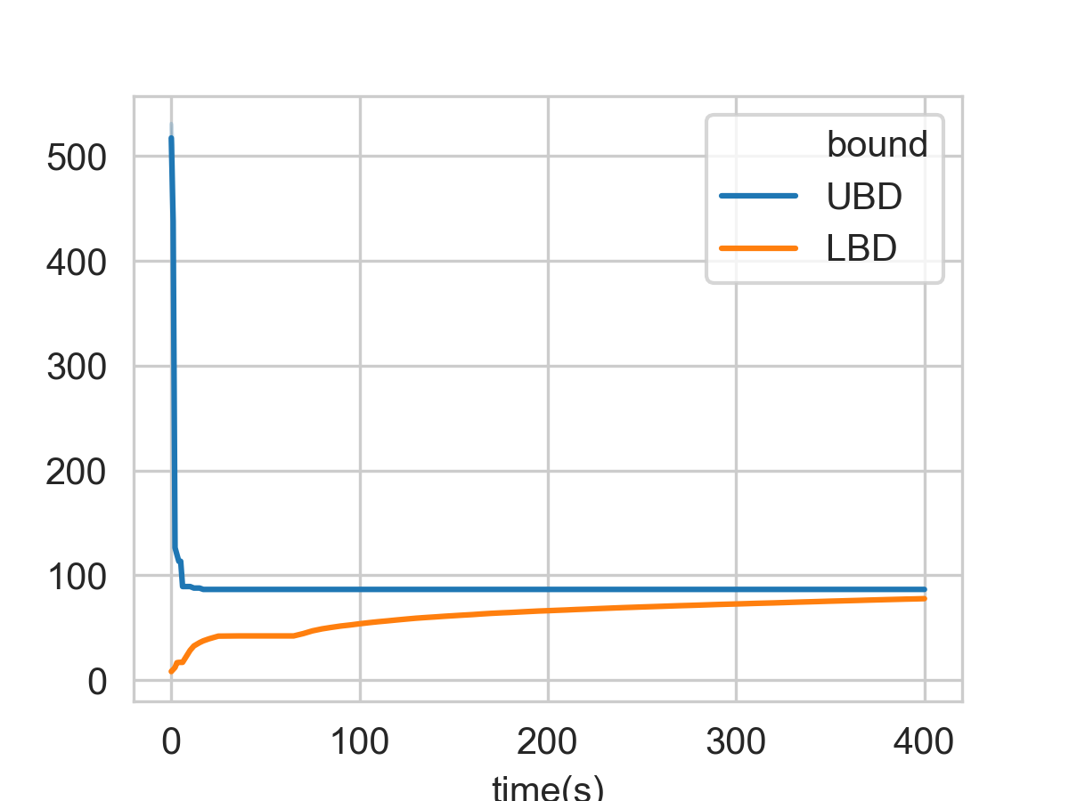
(a) Convergence of upper and lower bounds for MINLP method shows that optimal solution is found quickly, with the majority of time is spent proving global optimality of the MAP estimate.

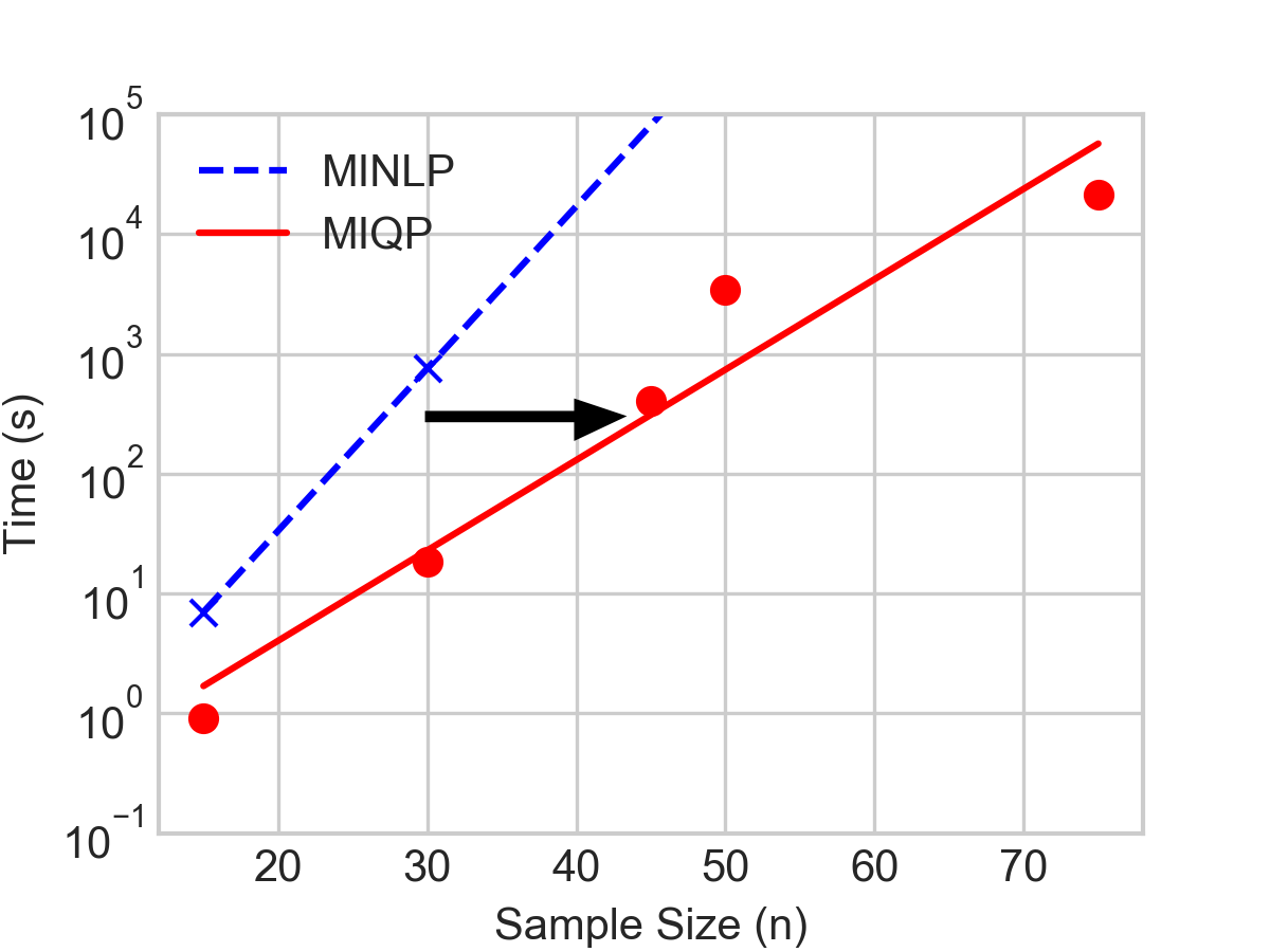
(b) Our MIQP approach improves upon the MINLP solution computation time as shown by the shift of the computation (log) time versus sample size curve to the right.

Figure 1: Global Convergence of MINLP and Time Comparison between MINLP and MIQP

Table 2 shows the comparison of our proposed branch-and-bound methods (MINLP, MIQP) with standard local search methods (EM, SLSQP, SA). Our primary interest lies in achieving a measure of convergence to the global optimum and the relative gap indicates the proximity of the upper and lower bounds. On all of the data sets, all methods find roughly the same optimal value. The MINLP method consistently has a fairly large gap and the MIQP method has a much smaller gap indicating that it provides a tighter bound on the globally optimal value.

Table 2: Comparison of expectation-maximization (EM), sequential least squares programming (SLSQP), basin-hopping simulated annealing (SA), branch-and-bound on the MINLP using BARON (MINLP), branch-and-bound on the MIQP using Gurobi (MIQP). The solution reported for MINLP and MIQP are the best feasible solution found within time limit. The total variation distance metric is used for $\bm{\pi}$, the $L_{2}$ distance is used for $\bm{\mu}$, and the average (across samples) total variation distance is used for $\bm{z}$.

		Local				Global (BnB)
Data Set	Metric	EM	SLSQP	SA		MINLP	MIQP
iris (1 dim)	$-\log$ MAP	280.60	287.44	283.28		280.02	282.71
	LBD	—	—	—		9.27	161.60
	$\sup|\hat{\bm{\pi}}-\bm{\pi}|$	0.075	0.013	0.000		0.093	0.165
	$\|\hat{\bm{\mu}}-\bm{\mu}\|_{2}$	0.278	0.065	0.277		0.356	0.356
	$\nicefrac{{1}}{{n}}\sum_{i}\sup|\hat{\bm{z}_{i}}-\bm{z}_{i}|$	0.067	0.067	0.087		0.093	0.093
wine (13 dim)	$-\log$ MAP	1367.00	1368.71	1368.71		1366.85	1390.13
	LBD	—	—	—		$-2.2\text{\times}{10}^{5}$	183.42
	$\sup|\hat{\bm{\pi}}-\bm{\pi}|$	0.005	0.066	0.066		0.006	0.167
	$\|\hat{\bm{\mu}}-\bm{\mu}\|_{2}$	2.348	1.602	1.652		1.618	14.071
	$\nicefrac{{1}}{{n}}\sum_{i}\sup|\hat{\bm{z}_{i}}-\bm{z}_{i}|$	0.006	0.006	0.006		0.006	0.022
brca (3 dim)	$-\log$ MAP	1566.49	1662.97	1662.97		1566.40	1578.49
	LBD	—	—	—		$-2.7\text{\times}{10}^{4}$	332.30
	$\sup|\hat{\bm{\pi}}-\bm{\pi}|$	0.167	0.127	0.127		0.169	0.122
	$\|\hat{\bm{\mu}}-\bm{\mu}\|_{2}$	394.07	321.11	320.60		401.47	418.05
	$\nicefrac{{1}}{{n}}\sum_{i}\sup|\hat{\bm{z}_{i}}-\bm{z}_{i}|$	0.169	0.139	0.139		0.169	0.174

EM algorithm with multiple restarts

We explored whether the EM algorithm can identify the global optimum if restarted multiple times from random initial values. We restarted the EM algorithm and ran to convergence for 12 hours and retained the best local MAP value. For the iris1d data set with $n=45$, the best local MAP identified by the EM algorithm was 194.9582 and the global MAP identified by MIQP was 194.9455. The global MAP clustering was identified by the MIQP algorithm in 17 seconds, an additional 125.19 seconds were spent proving global optimality (converging the lower bound as shown in Figure 1(a)). This shows that EM may get trapped in attractive, albeit local, minima, and so is unable to prove global optimality.

Comparison to Bandi et. al.

We implemented the Bandi et al., (2019) method with the Kolmogorov-Smirnov distance as the discrepancy measurement and set the stopping criterion to $\epsilon=0.01$. The in-sample cluster assignment accuracy on the iris1d and brca data sets are 90.0% and 74.4% using Bandi et al., (2019). For the wine data set, the clustering accuracy is 58.4%. Our implementation matches the results reported in Bandi et al., (2019) for iris and brca; they did not report results on wine. In comparison, Table 2 shows that our in-sample assignment accuracy is 90.7%, 83.1% and 99.4% for iris1d, brca, and wine. To test whether the discrepancy on the wine data set is due to the estimation of the variance parameters, we fixed the variance parameters and cluster proportion parameters to their true values for the Bandi et al., (2019) method. The cluster assignment accuracy improved but still does not achieve the same level of accuracy as our MIQP method. The remaining possible causes for the discrepancy are that the Bandi et al., (2019) method uses the Kolmogorov-Smirnov distance or total variation distance to estimate parameters rather than maximum likelihood or maximum a posteriori cluster assignments. To underscore the fundamental difference between our approaches, our approach is focused on the in-sample cluster assignment—an important problem in Bayesian statistics and biological data analysis, whereas the Bandi et al., (2019) approach is focused on the out-of-sample prediction problem—a different, but no less important problem.

4.2 Clustering Breast Cancer Gene Expression Data

We evaluated our proposed approach on Prediction Analysis of Microarray 50 (pam50) gene expression data set. The PAM50 gene set is commonly used to identify the “intrinsic” subtypes of breast cancer among luminal A (LumA), luminal B (LumB), HER2-enriched (Her2), basal-like (Basal), and normal-like (Normal). Different subtypes lead to different treatment decisions, so it is critical to identify the correct subtype. The PAM algorithm finds centroids under a Spearman’s rank correlation distance (Tibshirani et al.,, 2002; Parker et al.,, 2009). Our primary interest with the experiment is to show the effects of incorporating constraints into the clustering problem. In this data set, we have important side information that we incorporate and find that it significantly improves computational time and accuracy.

Data collection and preprocessing

We used the pam50 data set ($n=232$, $d=50$) obtained from UNC MicroArray Database (University of North Carolina,, 2020). The pam50 dataset contains 139 subjects whose intrinsic subtypes are known, and 93 subjects whose intrinsic subtypes are unknown. Missing data values (2.65%) were filled in with zeros. A 4-d projection of pam50 was obtained by projecting on the first 4 principal components (designated pam50-4d), preserving 58.6% of the information variation. The precision matrix was fixed to the average of the estimates intrinsic subtype component precision matrices.

Experimental Protocol

We ran the PAM algorithm using R code provided by the authors as supplementary material. MINLP and MIQP methods employed additional constraints to Problem (1) such that 139 samples were assigned to known subtypes. All variants of our approaches were implemented in the same environment described in Section 4.1, except MIQP was run on 32 cores.

Hard constraints improve computational time

We assessed convergence to the global optimum for the pam50-4d data set using MIQP with and without the constraints on 139 samples with known intrinsic subtypes. Without constraints, the optimality gap was 99.83%, and the addition of constraints allowed the method to achieve a 32.35% optimality gap for the same computation time. The incorporation of hard constraints greatly improves the computational efficiency.

Comparison to PAM algorithm

Figure 2 shows a comparison of cluster assignments of our methods (MINLP, MIQP) with the PAM algorithm. For 139 samples with known instrinsic subtypes, assignments from MINLP and MIQP methods have 100% accuracy, while PAM accuracy is 94%. This is due to the capability of MINLP and MIQP to incorporate prior constraints in the clustering problem. For the 93 samples with unknown subtypes, MINLP assignments have 68% concordance with the PAM algorithm, and MINLP has 89% concordance with MIQP assignments.

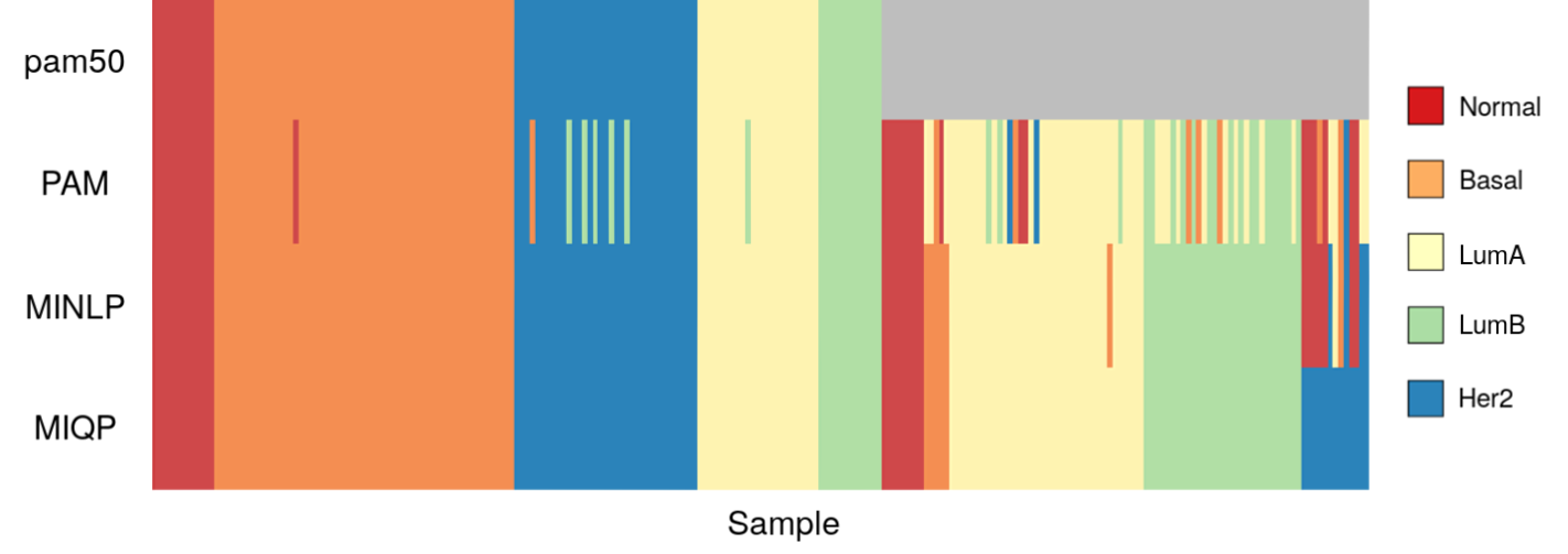
Figure 2: Breast cancer intrinsic subtypes assignments. pam50 shows true assignments for 139 samples and unknown assignments (gray) for 93 samples. PAM is the centroid algorithm in Tibshirani et al., (2002); MINLP and MIQP are our methods.

Biological interpretation of MIQP and PAM cluster assignments

We selected two samples that were assigned to different clusters by the PAM algorithm and our MIQP method to explore whether the cluster assignments made by MIQP are more or less biologically meaningful (see Supplementary Material for plots of other samples). Figure 3 shows the gene expression profile for sample 13 which has a known intrinsic subtype (Figure 3(a)) and sample 24 which has an unknown intrinsic subtype (Figure 3(b)).

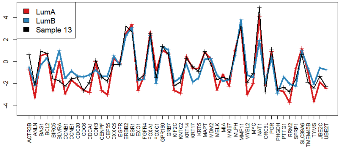
(a) Gene expression data comparison of sample 13, average of LumA and average of LumB. The true subtype is LumA, MIQP correctly assigned it to LumA, and PAM incorrectly assigned it to LumB.

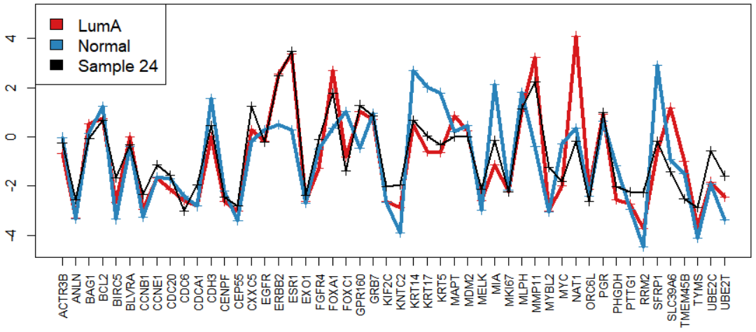
(b) Gene expression data comparison of sample 24, average of LumA, and average of Normal. The true subtype is unidentified, MIQP assigned it to LumA, and PAM assigned it to Normal.

Figure 3: Comparison of gene expression profiles with average intrinsic subtype profiles for samples 13 and 24.

Sample 13 is known to be a Luminal A (LumA) subtype and is correcty assigned to LumA by the MIQP method, but incorrectly assigned to LumB by PAM. The expression profile clearly matches the LumA average more closely for CCNB1, CCNE1, CDC6 and NAT1. NAT1 has been shown to be elevated in individuals with estrogen receptor positive (ER+) breast cancers (Wang et al.,, 2019) and 30-45% of Luminal A cancers are ER+ (Voduc et al.,, 2010). Therefore, the assignment to Luminal A is more biologically consistent.

Sample 24 is an unknown intrinsic subtype in the pam50 data set; it is assigned to the Normal subtype by the PAM algorithm and to the LumA subtype by the MIQP method. Clearly, the expression profile of the unknown sample shows an overexpression of ERBB2, ESR1, and the KRT cluster (KRT14, KRT17, and KRT5) which are consistent with the average LumA expression profile and inconsistent with the average Normal expression profile. ERBB2 is commonly known as HER2 and overexpression of HER2 would indicate the sample might be assigned to the HER2 intrinsic subtype. The moderate keratin (KRT) expression levels (KRT14, KRT17, KRT5) are clearly more consistent with LumA (overexpression has been associated with the basal subtype (Fredlund et al.,, 2012; Gusterson et al.,, 2005)). Even though the expression of the NAT1 gene in the unknown sample is different than the LumA average, the overall pattern of expression is consistent with LumA. All of this evidence suggests that this sample may be heterogeneous with multiple oncogenic driving events (including HER2 overexpression); and it is almost certainly not Normal.

5 Discussion

We formulated the MAP clustering problem as an MINLP and cast several local MAP clustering methods in the framework of the MINLP. We identified three aspects of the MINLP that can be adjusted to incorporate prior information and improve computational efficiency. We suggested an approximation that transforms the MINLP to an MIQP and offers control over the approximation error at the expense of computational time. We applied our approach to a real breast cancer clustering data set and found that incorporating hard constraints in our method significantly both improves computational time and biological interpretation of the resulting sample assignments.

Appendix A Biconvex MINLP Proof

In this section we define the biconvex mixed-integer nonlinear programming problem and show that Problem (1) is such a problem. In Section A.1, we review the definitions related to mixed-integer nonlinear optimization. Then, in Section A.2 we define the biconvex optimization problem. Finally, in Section A.3 we extend definitions from Section A.1 and Section A.2 and apply them to Problem (1).

A.1 Mixed-Integer Nonlinear Optimization

Definition A.1 (MINLP).

A mixed-integer nonlinear programming problem is of the form x, yf(x, y) g(x, y)≤0 h(x, y)= 0 where $x\in\mathcal{X}\subseteq\mathbb{R}^{n}$, $y\in\mathcal{Y}\subseteq\mathbb{Z}^{m}$, $f:\mathbb{R}^{n}\times\mathbb{R}^{m}\rightarrow\mathbb{R}$, $\bm{g}:\mathbb{R}^{n}\times\mathbb{R}^{m}\rightarrow\mathbb{R}^{p}$, and $\bm{h}:\mathbb{R}^{n}\times\mathbb{R}^{m}\rightarrow\mathbb{R}^{q}$ (Belotti et al.,, 2013).

Definition A.2 (Convex MINLP).

Problem (A.1) is a convex MINLP if $f$ is separable and linear, $f(\bm{x},\bm{y})=\bm{c}_{1}^{T}\bm{x}+\bm{c}_{2}^{T}\bm{y}$, and the constraints $g_{j}$ are jointly convex in $\bm{x}$ and the relaxed integer variables $y_{i}\in[0,1]$ for all $j$ and $i$ (Kronqvist et al.,, 2019).

A.2 Biconvex Optimization

Definition A.3 (Biconvex Set).

The set $\mathcal{B}\subseteq\mathcal{X}\times\mathcal{Y}$ is called a biconvex set on $\mathcal{X}\times\mathcal{Y}$ or biconvex if $\mathcal{B}_{\bm{x}}$ is convex for every $\bm{x}\in\mathcal{X}$ and $\mathcal{B}_{\bm{y}}$ is convex for every $\bm{y}\in\mathcal{Y}$ (Gorski et al.,, 2007). The $x-$ and $y-$ sections of $\mathcal{B}$ are defined as $\mathcal{B}_{x}=\{\bm{y}\in\mathcal{Y}:(\bm{x},\bm{y})\in\mathcal{B}\}$ and $\mathcal{B}_{y}=\{\bm{x}\in\mathcal{X}:(\bm{x},\bm{y})\in\mathcal{B}\}$ respectively.

Definition A.4 (Biconvex Function).

A function $f:\mathcal{B}\rightarrow\mathbb{R}$ on a biconvex set $\mathcal{B}\subseteq\mathcal{X}\times\mathcal{Y}$ is a biconvex function on $\mathcal{B}$ if $f_{\bm{x}}(\bullet)=f(\bm{x},\bullet):\mathcal{B}_{\bm{x}}\rightarrow\mathbb{R}$ is a convex function on $\mathcal{B}_{\bm{x}}$ for every fixed $\bm{x}\in\mathcal{X}$ and $f_{\bm{y}}(\bullet)=f(\bullet,\bm{y}):\mathcal{B}_{\bm{y}}\rightarrow\mathbb{R}$ is a convex function on $\mathcal{B}_{\bm{y}}$ for every fixed $\bm{y}\in\mathcal{Y}$ (Gorski et al.,, 2007).

Definition A.5 (Biconvex Optimization Problem).

The problem $\min f(\bm{x},\bm{y}):(\bm{x},\bm{y})\in\mathcal{B}$ is a biconvex optimization problem if the feasible set $\mathcal{B}$ is biconvex on $\mathcal{X}\times\mathcal{Y}$ and the objective function $f$ is biconvex on $\mathcal{B}$ (Gorski et al.,, 2007).

A.3 Biconvex Mixed-Integer Nonlinear Optimization

Definition A.6 (Biconvex MINLP).

The problem x, yf(x, y) g(x, y)≤0 h(x, y)= 0 is a biconvex MINLP if the feasible set $\mathcal{B}$ and the objective function $f$ are biconvex in $\bm{x}$ and the relaxed integer variables $y_{i}\in[0,1]$.

Theorem 2.

Maximum a posteriori estimation for the Gaussian mixture model (1) with known covariance is a biconvex mixed-integer nonlinear programming optimization problem.

Proof.

The structure of the proof is to first relax the binary variables such that $y_{i}\in[0,1]$. Then show the feasible set $\mathcal{B}$ is biconvex. Finally show the objective function is biconvex.

The relaxed maximum a posterior estimation problem is |s| z, μ, π η∑_i=1^n ∑_k=1^K z_ik (y_i - μ_k)^2 - ∑_i=1^n ∑_k=1^K z_ik logπ_k ∑_k=1^K π_k=1 ∑_k=1^K z_ik=1, i=1,…,n -M_k^L ≤μ_k≤M_k^U, k=1,…,K π_k≥0, k=1,…,K z_ik∈[0,1], i=1, …, n k=1, …, K. For the remainder we consider range of the objective function to be the extended reals $\mathbb{R}\cup\{-\infty,\infty\}$ to simplify the case when $\pi_{k}=0$ for any $k$.

Feasible Set is Biconvex

It is easy to see that the feasible set is convex in $(\bm{\pi},\bm{\mu})$ for fixed $\bm{z}$ because $\bm{\pi}$ is in the $K$-dimensional simplex and the constraints on $\bm{\mu}$ are box constraints. Likewise, the constraints on $\bm{z}$ are trivially convex for fixed $(\bm{\pi},\bm{\mu})$.

Objective Function is Biconvex

As in Problem (1), we consider $\eta$ to be known. For fixed $\bm{z}$, the objective function is the linear combination of a quadratic term in $\bm{\mu}$ and a convex $-\log$ term in $\bm{\pi}$. Therefore the objective function is convex in $(\bm{\pi},\bm{\mu})$ for fixed $\bm{z}$. For fixed $(\bm{\pi},\bm{\mu})$, the objective function is linear in $\bm{z}$ and therefore convex. Therefore, the objective function is biconvex. ∎

Appendix B Branch-and-Bound Algorithm

The general branch-and-bound algorithm is outlined in Algorithm 1.

  Initialize the candidate priority queue to consist of the relaxed MINLP and set $\text{UBD}=\infty$ and $\text{GLBD}=-\infty$

  while candidate queue is not empty do

     Pop the first node off of the priority queue, solve the subproblem, and store the optimal value $f^{*}$.

     if $\bm{z}$ integral then

        if $f^{*}\leq\textrm{UBD}$ then

           Update $\text{UBD}\leftarrow f^{*}$

           Remove node $j$ from candidate queue where $\textrm{LBD}_{j}>\textrm{UBD}\ \forall j$

        end if

     else

        Select a branching variable $z_{ik}$ according to branching strategy

        Push node for candidate relaxed subproblem $j$ on queue adding constraint $z_{ik}=0$ and set $\textrm{LBD}_{j}=f^{*}$

        Push node for candidate relaxed subproblem $j^{\prime}$ on queue adding constraint $z_{ik}=1$ and set $\textrm{LBD}_{j^{\prime}}=f^{*}$

     end if

     Set $\text{GLBD}=\min_{j}\text{LBD}_{j}$ for all $j$ in candidate queue

  end while

Algorithm 1 Branch-and-Bound

B.1 Branching Strategies

Though the choice of branching strategy should be tailored to the problem, there are three popular general strategies (Achterberg et al.,, 2005): Most Infeasible Branching – choose the integer variable with the fraction part closest to 0.5 in the relaxed subproblem solution, Pseudo Cost Branching — choose the variable that provided the greatest reduction in the objective when it was previously branched on in the tree, and Strong Branching — test a subset of the variables at both of their bounds and branch on the one that provides the greatest reduction in the objective function.

The strong branching strategy can be computationally expensive because two optimization problems must be solved for each candidate, so loose approximations such as linear programs are often used. The pseudo cost strategy does not provide much benefit early in the iterations because there is not much branching history to draw upon. Rather than using a general-purpose strategy, we have developed a branching strategy more tuned for the finite mixture model problem.

Most Integral Branching

We implemented a most integral branching strategy for the GMM MAP problem. The idea is to first find a solution to a relaxed problem where $z_{ik}\in[0,1]$. Then, identify those $z_{ik}$ variables that are closest to 1 — that is, variables that are most definitively assigned to one component. Those $z_{ik}$ variables are then chosen for branching with the expectation that the relaxed subproblem branch with the constraint that $z_{ik}=0$ will tend to have a lower bound that is greater than the best upper bound and the subtree can be fathomed.

B.2 Algorithm Strategies

The general branch-and-bound algorithm (Algorithm 1) is implemented as a tree with nodes indexed in a priority queue. A node in the candidate priority queue contains a relaxed subproblem and a lower bound for the subproblem. Each branching leads to a child node subproblem. If a lower bound of a child node is greater than the best current upper bound, then the subtree is fathomed and the search space is reduced by a factor of up to one half, drastically improving the computational efficiency. Given Theorem 1 the subproblem at each node is a biconvex nonlinear programming problem.

Appendix C Comparison of Gene Expression Profiles

In our experiments 45 samples were classified differently by PAM and our MIQP method. Here we show how the samples were assigned and plots of the expression profile for the sample and the average of the expression profile of the two assignments.

Table 3: Comparison of assignments of samples who are assigned to different subtypes from PAM and MIQP.

Sample	PAM Assignment	MIQP Assignment
Sample 1	Normal	Her2
Sample 2	LumA	Her2
Sample 3	Basal	Her2
Sample 4	Normal	Her2
Sample 5	Normal	Her2
Sample 6	Normal	Basal
Sample 7	Basal	Her2
Sample 8	LumB	Her2
Sample 9	LumB	Her2
Sample 10	LumB	Her2
Sample 11	LumB	Her2
Sample 12	LumB	Her2
Sample 13	LumB	LumA
Sample 14	LumA	Basal
Sample 15	LumA	Her2
Sample 16	LumA	LumB
Sample 17	LumA	Basal
Sample 18	LumA	LumB
Sample 19	LumB	LumA
Sample 20	LumB	LumA
Sample 21	Her2	LumA
Sample 22	Basal	LumA
Sample 23	LumA	LumB
Sample 24	Normal	LumA
Sample 25	Normal	LumA
Sample 26	LumA	LumB
Sample 27	Basal	LumB
Sample 28	Her2	LumA
Sample 29	Basal	LumB
Sample 30	LumA	LumB
Sample 31	Basal	LumB
Sample 32	LumA	LumB
Sample 33	LumA	LumB
Sample 34	LumA	LumB
Sample 35	LumA	LumB
Sample 36	Normal	Basal
Sample 37	LumA	Her2
Sample 38	LumB	LumA
Sample 39	LumA	Basal
Sample 40	LumA	Her2
Sample 41	LumA	LumB
Sample 42	Normal	Her2
Sample 43	Normal	Her2
Sample 44	Normal	Her2
Sample 45	Basal	Her2

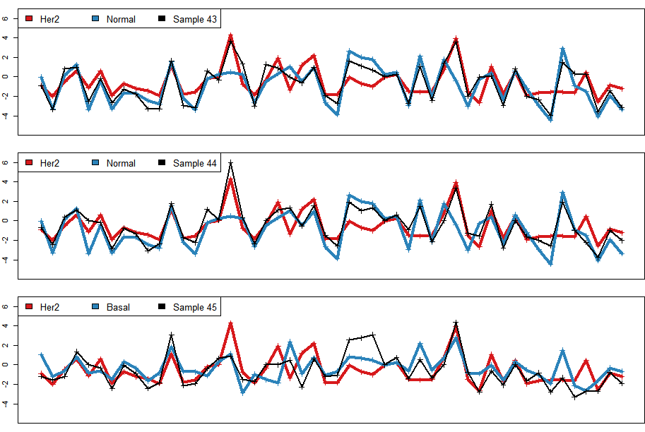
Figure 4: Comparison of gene expression profiles of samples that are assigned to different subtypes from PAM and MIQP. The x-axis is the genes in the PAM50 signature shown in Figure 3.

References

- Achterberg et al., (2005) Achterberg, T., Koch, T., and Martin, A. (2005). Branching rules revisited. Operations Research Letters, 33(1):42–54.
- Andrieu et al., (2003) Andrieu, C., de Freitas, N., Doucet, A., and Jordan, M. I. (2003). An introduction to MCMC for machine learning. Machine Learning, 50(1):5–43.
- Balakrishnan et al., (2017) Balakrishnan, S., Wainwright, M. J., and Yu, B. (2017). Statistical guarantees for the EM algorithm: From population to sample-based analysis. Ann. Statist., 45(1):77–120.
- Bandi et al., (2019) Bandi, H., Bertsimas, D., and Mazumder, R. (2019). Learning a mixture of gaussians via mixed-integer optimization. Informs Journal on Optimization, 1(3):221–240.
- Beal and Ghahramani, (2003) Beal, M. J. and Ghahramani, Z. (2003). The variational Bayesian EM algorithm for incomplete data: with application to scoring graphical model structures. In Bernardo, J., Bayarri, M., Berger, J., Dawid, A., Heckerman, D., Smith, A., and West, M., editors, Bayesian Statistics 7: Proceedings of the Seventh Valencia International Meeting, volume 7, pages 453–464. Oxford University Press.
- Belotti et al., (2013) Belotti, P., Kirches, C., Leyffer, S., Linderoth, J., Luedtke, J., and Mahajan, A. (2013). Mixed-integer nonlinear optimization. Acta Numerica, pages 1–131.
- Bertsimas and King, (2016) Bertsimas, D. and King, A. (2016). OR forum–An algorithmic approach to linear regression. Operations Research, 64(1):2–16.
- Bertsimas and King, (2017) Bertsimas, D. and King, A. (2017). Logistic regression: From art to science. Statistical Science, 32(3):367–384.
- Bertsimas et al., (2016) Bertsimas, D., King, A., and Mazumder, R. (2016). Best subset selection via a modern optimization lens. The Annals of Statistics, 44(2):813–852.
- Bertsimas and Li, (2020) Bertsimas, D. and Li, M. L. (2020). Scalable holistic linear regression. Operations Research Letters.
- Bisschop and Meeraus, (1982) Bisschop, J. and Meeraus, A. (1982). On the Development of a General Algebraic Modeling System in a Strategic Planning Environment. In Applications, volume 20 of Mathematical Programming Studies, pages 1–29. Springer Berlin Heidelberg.
- Bodic and Nemhauser, (2015) Bodic, P. L. and Nemhauser, G. L. (2015). How important are branching decisions: Fooling MIP solvers. Operations Research Letters, 43(3):273–278.
- Braun and McAuliffe, (2010) Braun, M. and McAuliffe, J. (2010). Variational inference for large-scale models of discrete choice. Journal of the American Statistical Association, 105(489):324–335.
- Cochran, (2018) Cochran, J. J. (2018). INFORMS Analytics Body of Knowledge. John Wiley & Sons.
- Dua and Graff, (2017) Dua, D. and Graff, C. (2017). UCI machine learning repository.
- Floudas, (2000) Floudas, C. A. (2000). Deterministic Global Optimization. Nonconvex Optimization and Its Applications. Springer US.
- Fredlund et al., (2012) Fredlund, E., Staaf, J., Rantala, J. K., Kallioniemi, O., Borg, Å., and Ringnér, M. (2012). The gene expression landscape of breast cancer is shaped by tumor protein p53 status and epithelial-mesenchymal transition. Breast Cancer Research, 14(4):R113.
- GAMS Development Corporation, (2017) GAMS Development Corporation (2017). GAMS — A User’s Guide. GAMS Development Corporation.
- Gelman and Rubin, (1996) Gelman, A. and Rubin, D. B. (1996). Markov Chain Monte Carlo methods in biostatistics. Statistical Methods in Medical Research, 5(4):339–355.
- Glover, (1975) Glover, F. (1975). Improved linear integer programming formulations of nonlinear integer problems. Management Science, 22(4):455–460.
- Gorski et al., (2007) Gorski, J., Pfeuffer, F., and Klamroth, K. (2007). Biconvex sets and optimization with biconvex functions: a survey and extensions. Mathematical Methods of Operations Research, 66(3):373–407.
- Greenberg et al., (2019) Greenberg, C., Monath, N., Kobren, A., Flaherty, P., McGregor, A., and McCallum, A. (2019). Compact representation of uncertainty in clustering. In Proceedings of the Neural Information Processing Systems Meeting.
- Grötschel, (2012) Grötschel, M. (2012). Optimization stories. Dt. Mathematiker-Vereinigung.
- Gurobi Optimization, (2018) Gurobi Optimization, L. (2018). Gurobi Optimizer reference manual.
- Gusterson et al., (2005) Gusterson, B. A., Ross, D. T., Heath, V. J., and Stein, T. (2005). Basal cytokeratins and their relationship to the cellular origin and functional classification of breast cancer. Breast Cancer Research, 7(4):143.
- Jin et al., (2016) Jin, C., Zhang, Y., Balakrishnan, S., Wainwright, M. J., and Jordan, M. I. (2016). Local maxima in the likelihood of Gaussian mixture models: Structural results and algorithmic consequences. In Proceedings of the 30th International Conference on Neural Information Processing Systems, NIPS’16, pages 4123–4131, USA. Curran Associates Inc.
- Kronqvist et al., (2019) Kronqvist, J., Bernal, D. E., Lundell, A., and Grossmann, I. E. (2019). A review and comparison of solvers for convex MINLP. Optimization and Engineering, 20(2):397–455.
- Land and Doig, (1960) Land, A. H. and Doig, A. G. (1960). An automatic method of solving discrete programming problems. Econometrica, 28(3):497.
- Lange et al., (2000) Lange, K., Hunter, D. R., and Yang, I. (2000). Optimization transfer using surrogate objective functions. Journal of Computational and Graphical Statistics, 9(1):1.
- Magnani and Boyd, (2008) Magnani, A. and Boyd, S. P. (2008). Convex piecewise-linear fitting. Optimization and Engineering, 10(1):1–17.
- Mairal, (2013) Mairal, J. (2013). Optimization with first-order surrogate functions. In Proceedings of the 30th International Conference on Machine Learning.
- Murty and Kabadi, (1987) Murty, K. G. and Kabadi, S. N. (1987). Some NP-complete problems in quadratic and nonlinear programming. Mathematical Programming, 39(2):117–129.
- Nemhauser and Wolsey, (1988) Nemhauser, G. and Wolsey, L. (1988). Integer and Combinatorial Optimization. John Wiley & Sons, Inc.
- Nocedal and Wright, (2006) Nocedal, J. and Wright, S. J. (2006). Numerical optimization. Springer, New York.
- Parker et al., (2009) Parker, J. S., Mullins, M., Cheang, M. C., Leung, S., Voduc, D., Vickery, T., Davies, S., Fauron, C., He, X., Hu, Z., Quackenbush, J. F., Stijleman, I. J., Palazzo, J., Marron, J., Nobel, A. B., Mardis, E., Nielsen, T. O., and J, M. (2009). Supervised risk predictor of breast cancer based on intrinsic subtypes. Journal of Clinical Oncology, pages 1160–1167.
- Sahinidis, (2017) Sahinidis, N. V. (2017). BARON 17.8.9: Global Optimization of Mixed-Integer Nonlinear Programs, User’s Manual.
- Tawarmalani and Sahinidis, (2005) Tawarmalani, M. and Sahinidis, N. V. (2005). A polyhedral branch-and-cut approach to global optimization. Mathematical Programming, 103(2):225–249.
- Tibshirani et al., (2002) Tibshirani, R., Hastie, T., Narasimhan, B., and Chu, G. (2002). Diagnosis of multiple cancer types by shrunken centroids of gene expression. PNAS, pages 6567–6572.
- University of North Carolina, (2020) University of North Carolina (2020). UNC microarray database. https://genome.unc.edu/.
- Voduc et al., (2010) Voduc, K. D., Cheang, M. C., Tyldesley, S., Gelmon, K., Nielsen, T. O., and Kennecke, H. (2010). Breast cancer subtypes and the risk of local and regional relapse. Journal of clinical oncology, 28(10):1684–1691.
- Wainwright and Jordan, (2007) Wainwright, M. J. and Jordan, M. I. (2007). Graphical models, exponential families, and variational inference. Foundations and Trends® in Machine Learning, 1(1-2):1–305.
- Wales and Doye, (1997) Wales, D. J. and Doye, J. P. K. (1997). Global optimization by basin-hopping and the lowest energy structures of Lennard-Jones clusters containing up to 110 atoms. The Journal of Physical Chemistry A, 101(28):5111–5116.
- Wang and Blei, (2013) Wang, C. and Blei, D. M. (2013). Variational inference in nonconjugate models. J. Mach. Learn. Res., 14(1):1005–1031.
- Wang et al., (2019) Wang, L., Minchin, R. F., Essebier, P. J., and Butcher, N. J. (2019). Loss of human arylamine n-acetyltransferase I regulates mitochondrial function by inhibition of the pyruvate dehydrogenase complex. The international journal of biochemistry & cell biology, 110:84–90.