Methods for Stabilizing Models across Large Samples of Projects
 (with case studies on Predicting Defect and Project Health)

Abstract.

Despite decades of research, SE lacks widely accepted models (that offer precise quantitative stable predictions) about what factors most influence software quality. This paper provides a promising result showing such stable models can be generated using a new transfer learning framework called “STABILIZER”. Given a tree of recursively clustered projects (using project meta-data), STABILIZER promotes a model upwards if it performs best in the lower clusters (stopping when the promoted model performs worse than the models seen at a lower level).

The number of models found by STABILIZER is minimal: one for defect prediction (756 projects) and less than a dozen for project health (1628 projects). Hence, via STABILIZER, it is possible to find a few projects which can be used for transfer learning and make conclusions that hold across hundreds of projects at a time. Further, the models produced in this manner offer predictions that perform as well or better than the prior state-of-the-art.

To the best of our knowledge, STABILIZER is order of magnitude faster than the prior state-of-the-art transfer learners which seek to find conclusion stability, and these case studies are the largest demonstration of the generalizability of quantitative predictions of project quality yet reported in the SE literature.

In order to support open science, all our scripts and data are online at https://github.com/Anonymous633671/STABILIZER.

1. Introduction

The mining methods presented at the MSR conference are excellent for building models specific to individual projects. These models cover many diverse tasks such as the detection of code smells, code refactoring (Tufano et al., 2015; Mantyla et al., 2004; Sjøberg et al., 2012) or the two case studies explored in this paper: defect prediction (Ostrand et al., 2004; Ghotra et al., 2015; Zimmermann et al., 2009; Yang et al., 2017) and software project health estimation (Link and Germonprez, 2018; Wynn Jr, 2007; Crowston and Howison, 2006). Better yet, when some specialized effect holds for one project, then our data mining methods can reveal that effect by creating a model that is exactly suited to that project. Further, when the effect changes (say, in next release), our mining methods can be run again to learn yet another model that is specialized for the new current state of the project.

But this “specialization effect” raises its own challenges. If every model we build is specialized to just the latest data from some current project, then it becomes hard to claim general results that hold across multiple projects. Hassan (Hassan, 2017) warns that managers lose trust in software analytics if the results keep changing.

We raise this concern since, the usual result is that the models build via data mining for SE data are not stable across multiple projects (see §2 and (Zimmermann et al., 2009; Menzies et al., 2013, 2011)). When different projects result in different models, it is hard to gain insights about what affects software quality. This is troubling, as Sawyer et al. (Sawyer, 2013) argue, such insights are the key driver for businesses. Generating new models each time we look at new data exhausts users’ ability to draw insight. Table 1 lists other problems caused by conclusion instability.

One way to find conclusions that hold across multiple projects is the “bellwether” method (Krishna and Menzies, 2018; Krishna et al., 2016a; Mensah et al., 2018, 2017a, 2017b). This method assumes that, given a community of projects, the “bellwether” is a project whose data yields the best analytic (i.e., defect prediction, effort estimation) on all others. This bellwether model can be used to generate stable conclusions across that community. However, current bellwether methods require an $O(N^{2})$ comparison of all models build from $N$ projects. Hence, that approach is hard to scale so prior bellwether papers on every reported generality across 20 projects (or less).

Table 1. There are many reasons to seek stable general conclusions in software engineering. If our conclusions about best practices for SE projects keep changing, that will be detrimental to generality trust, insight, training, and tool development.

Generality:	Data science for SE cannot be called a “science” until it makes general conclusions that hold across multiple projects. Without general rules for a large number of software projects, then it is difficult to demonstrate such generality.
Trust:	Hassan (Hassan, 2017) cautions that managers lose faith in software analytics if its models keep changing since the assumptions used to make prior policy decisions may no longer hold.
Insight:	Kim et al. (Kim et al., 2016), say that the aim of software analytics is to obtain actionable insights that help practitioners accomplish software development goals. These insights can be core deliverable (Tan and Chan, 2016), key driver for businesses  (Sawyer, 2013) or user reflections (Bird et al., 2015). But if new models keep being generated in new projects, then that exhausts the ability of users to draw insight from new data.
Training:	Another concern is what do we train novice software engineers or newcomers to a project? If our models are not stable, then it hard to teach what factors most influence software quality.
Tool development:	Further to the last point— if we are unsure what factors most influence quality, it is difficult to design and implement and deploy tools that can successfully improve that quality.

This paper proposed a novel framework called STABILIZER that works for 100s to 1000s of projects. STABILIZER uses hierarchical clustering. At each level of the cluster hierarchy, models “fight it out” to select a bellwether. The winner is promoted up the hierarchy and the process repeats. Sometimes this will return one model from the root of the hierarchy (in the case of defect prediction). And sometimes that promotion stops at some internal level (e.g., for project health estimation, we return around a dozen models). More importantly, STABILIZER indexes those models in its cluster tree so, when new projects arrive, they can explore down the cluster tree in log-time to find their relevant model.

To assess STABILIZER, we ask five questions:

RQ1: is STABILIZER tractable? Since one of our primary concern with prior work was its scalability, we are motivated to consider the computational cost of any new alternative. For $N$ projects recursively clustered into $m$ sub-groups, STABILIZER runs in time $\Theta(m*(N/m)^{2})$ (compared to $\Theta(N^{2})$ for prior work).

RQ2: is STABILIZER efficient? In practice, STABILIZER’s run-time increases less-than-linearly, compared to the prior SOTA in this area (Krishna and Menzies, 2018), as the project community size increases. Hence,STABILIZER scale much better than prior transfer learning methods. For example, in this paper, we can show STABILIZER results for 756 defect prediction data sets and 1628 effort estimation data sets. Those results were generated 29 to 104 times faster than Krishna et al.’s BELLWETHER algorithm (the prior SOTA in this area (Krishna and Menzies, 2018)).

RQ3: is STABILIZER effective? For all Github projects studied in this paper, the predictions made by the models generated for both case studies are better than the baseline and prior SOTA(SOTA) methods.

RQ4: is STABILIZER parsimonious? We show that the number of models generated in this manner is very small (one for defect prediction and less than a dozen for project health).

RQ5: What are the generalized feature we learned? We show that there are features which are important across a larger number of project and can be generalized across those projects.

Seeing these results, we can summarize our contributions as -

• A new, scalable, algorithm for transfer learning.

• To test that new algorithm, we offer two large case studies with 756 Github projects (for defect prediction) and 1628 Github projects (for project health estimation). To the best of our knowledge, these are the largest transfer learning experiments yet performed in the SE literature.

• In those case studies, our new method can generate better performing models that cover much more projects that seen before.

• We can show that STABILIZER’s new hierarchical transfer methods actually perform better traditional transfer learning methods, showing that prior transfer learning methods were not learning from enough projects.

• We can demonstrate the value of our new approach via its computational complexity and extensive experimentation.

The rest of this paper is structured as follows. After some background (in §2) we show two cases studies: defect prediction and effort estimation. §3 describes our new approach. §4 show our experimental rig , which is used to produce the results of §5.

2. Background

2.1. Why Study Conclusion Stability?

In this section, we justify why it is important to seek stable SE conclusions. Our concern will be with “conclusion instability” where conclusions change from one project to another. For a list of issues that are raised when conclusions are unstable, see Table 1.

Conclusion instability is well documented in the research community. Zimmermann et al. (Zimmermann et al., 2009) learned defect predictors from 622 pairs of projects (project1, project2). In only 4% of pairs, predictors from project1 worked on project2. Menzies et al. (Menzies et al., 2013) reported defect prediction results from 28 studies, most of which offered widely differing conclusions about what most influences defects.

Conclusion instability is also rampant in the developer community. Multiple studies report that human beliefs in software quality may often be inconsistent and even incorrect. Devanbu et al. (Devanbu et al., 2016; Bird et al., 2011) have conducted a case study among 564 Microsoft software developers to show that human beliefs on software quality can be quite varied and may not necessarily correspond with actual evidence within current projects. A more recent study by Shrikanth et al. (Shrikanth and Menzies, 2019) also reports such variability of human beliefs. They studied ten beliefs held by software developers about defect prediction, which were initially summarized by Wan et al. in 2018  (Wan et al., 2018). By measuring the actual support of these beliefs within the project, Shrikanth et al. found that among over 300,000 changes seen in different open-source projects, only 24% of the projects support all ten beliefs. Curiously, beliefs held by most developers do not necessarily have the most substantial support within projects. For example, according to Shrikanth et al., a belief acknowledged by 35% of the developers have the most support. In contrast, a belief held by 76% of the developers is only ranked 7th out of ten beliefs. Worse still, as a project grows to mature, the beliefs tend to be weakened rather than strengthened.

Such instability prevents project managers from offering clear guidelines on many issues, including (a) when a specific module should be inspected, (b) when modules should be refactored, and (c) deciding where to focus on expensive testing procedures. Bird et al. (Bird et al., 2015) notes that insights occur when users respond to software analytics models. Frequent model changes could exhaust users’ ability for confident conclusions from new data. Further, conclusion instability makes it hard to on-board novice engineers. It is hard to design and build appropriate tools for quality assurance activities without knowing what factors most influence the local project.

SE is conducted on ever-changing platforms using ever-changing tools by a constantly changing and evolving developer population of varying skills. Perhaps it is folly to assume one model can cover something as diverse as software engineering. But if we cannot remove instability, perhaps another tactic is to reduce it.

Maybe a better way to look at conclusion instability is to assume that - from 1000’s of projects- there might be small number of projects. Where each can act as stable model across a smaller community. In that view, we need tools that can find and index that small set of models that best represent the rest of the space; i.e. we need bellwethers.

What we show here is that we can reduce 1000s of projects to just a few dozen most representative examples. Dozens of models are still more than one, so developers and managers still need to be aware of (and debate) the aspects of their project that make it distinctive. That said, once we can summarize many projects into just a handful of models, then those debates need not be extensive. Further, when training engineers, we could present a small range of projects to them as part of their training.

2.2. Two Case Studies

In the following, we offer a hierarchical transfer learning framework for oyr three-step process. After hierarchically clustering the data, it replaces many models (in a sub-tree) with a single best model (selected from that sub-tree). This process then recurses up the tree of clusters. Sometimes this will return one model (in the case of defect prediction). If that is not possible, it will return multiple models (e.g., for project health estimation, we return around a dozen models). More importantly, STABILIZER indexes those models in its cluster tree. When new projects arrive, they can explore down the cluster tree in log-time to find their relevant model.

This novel approach is tested on the two case studies discussed in this section: defect prediction and project health estimation:

• Defect prediction (Ostrand et al., 2004; Ghotra et al., 2015; Zimmermann et al., 2009; Yang et al., 2017) prioritize where to look in a codebase such that more bugs are found sooner.

• Software project health estimation (Link and Germonprez, 2018; Wynn Jr, 2007; Crowston and Howison, 2006) incrementally monitors open-source projects (which is a very different process to classic waterfall up-front effort estimation (Kocaguneli et al., 2015; Boehm et al., 2000) that is conducted before developers start coding).

2.2.1. Why Defect Prediction?

The perceived criticality and bugginess of the code for managing resources efficiently are often associated with the QA effort. As bugs are not evenly distributed across the project (Hamill and Goseva-Popstojanova, 2009; Koru et al., 2009; Ostrand et al., 2004; Misirli et al., 2011), it is impractical and inefficient to distribute equal effort to every component in a software system (Briand et al., 1993). Algorithms that measure the criticality or bugginess of software using source code (product) or project history (process) are called defect prediction models. Although such defect predictors are never 100% correct, they can suggest where a defect might happen.

In a recent paper, Wan et al. (Wan et al., 2018), reported much industrial interest in these predictors since the alternative is much more time-consuming and expensive. Misirili et al. (Misirli et al., 2011) and Kim et al. (Kim et al., 2011) report considerable cost savings when such predictors are used in guiding industrial quality assurance processes.

As shown in Table 3 defect prediction models might use product or process metrics to make predictions. Process metrics comment on “who” and “how” the code was written, while product metrics record “what” was written. Researchers and industry practitioners have tried many different ways to identify which features are important and why. However, there is little agreement between them. Zimmermann et al. (Zimmermann et al., 2007) recommended complexity-based product metrics, Zhou et al. (Zhou et al., 2010) suggest size-based metrics. While Matsumoto et al. (Matsumoto et al., 2010), and Nagappan et al. (Nagappan et al., 2010) recommend developer-related metric and change bursts metrics, respectively. We use Table 3 metrics for both theoretical and pragmatic reasons. Our metrics include the process metrics endorsed by Devanbu et al. at ICSE’13 (Rahman and Devanbu, 2013).

2.2.2. Why Project Health?

Open-source software development is becoming prominent in the overall software engineering landscape. As the community matures, they become more structured with organizing foundations. Some prominent software organizations like Apache Foundation and Linux Foundation host hundreds of popular projects (Foundation, 2018, 2020). Stakeholders of these projects make critical decisions about the future of these projects based on project status. The metrics of project health conditions are needed when they estimate the projects. On the other hand, future customers thinking about using the open-source project in their product are more likely to invest and participate in “healthy” projects.

In the past decade, many researchers (Jarczyk et al., 2018; Kikas et al., 2016; Chen et al., 2014; Bidoki et al., 2018; Xia et al., 2020) have tried to look at project health from a different perspective. For example, Jansen et al. (Jansen, 2014) mentioned project could be estimated by the level of productivity, robustness, and niche of creation in the project history. Kikas et al. (Kikas et al., 2016) reported a relationship between the dynamic and contextual features of a project and issue close time. Wang et al. (Wang et al., 2018) and Bao et al. (Bao et al., 2019) proposed different predicting models to find potential long-term contributors. Jarczyk et al. (Jarczyk et al., 2018) use generalized linear models for the prediction of issue closure rate. Based on multiple features (i.e., stars, commits, issues closed), they find that larger teams with more project members have lower issue closure rates than smaller teams. At the same time, increased work centralization improves issue closure rates.

From January to March 2021, Xia (Xia, 2021) conducted email interviews with 116 subject matter experts from 68 open-source projects. One of the questions asked was “what kind of features are the most useful to predict for?”. In those answers, certain features were marked as the most important to that community: see Table 3. Note the “Predict?” column of that table: in our experiments, we take each prediction goal, one at a time, then try to predict for it using all the other metrics for six months into the future.

Table 2. List of metrics used in this study for defect prediction case study.

Metric	Description	Metric	Description
adev	Active Dev Count	nadev	Neighbor’s Active Dev Count
age	Interval between last, current change	ncomm	Neighbor’s Commit Count
ddev	Distinct Dev Count	nd	Number of Modified Directories
sctr	Distribution of modified code	nddev	Neighbor’s Distinct Dev Count
exp	Experience of the committer	ns	Number of Modified Subsystems
la	Lines of code added	nuc	Number of unique changes to files
ld	Lines of code deleted	own	Owner’s Contributed Lines
lt	Lines of code before the change	sexp	Developer experience on a subsystem
minor	Minor Contributor Count	rexp	Recent developer experience

Table 3. List of metrics used in this study for project health estimation case study.

Metric Category	Metric Name	Predict?
	MC: monthly number of commits	✓
Activeness	MAC: monthly number of active contributors	✓
	MOP: monthly number of open PRs	✓
	MCP :monthly number of closed PRs	✓
	MMP: monthly number of merged PRs
	MPM: monthly number of PR mergers
Collaboration	MPC: monthly number of PR comments
	MOI: monthly number of open issues	✓
	MCI: monthly number of closed issues	✓
	MIC: monthly number of issue comments
Enhancement
	MS: monthly increased number of stars	✓
	MF: monthly increased number of forks
Popularity	MW:monthly increased number of watchers

2.3. Transfer Learning

From a formal perspective, STABILIZER is a homogeneous, similarity-based, bellwether, transfer learning algorithm (and this section explains all the terms in italics.

The art of moving data and knowledge from one project or another is called transfer learning (Pan and Yang, 2009). When there is insufficient data to apply data miners, transfer learning can be used to transfer knowledge from other source projects to the target project. Clark and Madachy (Clark and Madachy, 2015) in their study showed developers working in an uncommon area often benefit from transferring knowledge from more common areas.

While transfer learning is widely studied and used in the software engineering domain, we warn that work mostly tries to move lessons learned from a single source project to a single target project, and these source projects changes for new target project. Hence, that research does not meet the goals of this paper (conclusion stability across 100s of projects). As discussed in the next section, additional engineering is required to convert current transfer learning tools for conclusion stability.

Transfer learning can be broadly categorized into two variants based on the similarity of features between source and target projects. Heterogeneous transfer learning is where the source and target data contains different attributes (Jing et al., 2015; He et al., 2014; Nam et al., 2017; Cheng et al., 2016; Yu et al., 2017). Homogeneous transfer learning is where the source and target data contains the same attributes (Ma et al., 2012a; Zimmermann et al., 2009; Turhan et al., 2009a; Krishna and Menzies, 2018). Our reproduction package for STABILIZER (listed on page1) collects the same set of attributes for all projects in both (a) defect prediction or (b) project health estimation case study. Hence, STABILIZER is a homogeneous transfer learner.

Another way to divide transfer learning is the approach that it follows. One is dimensional transformation methods, which manipulate the raw source data until it matches the target. Ma et al. (Ma et al., 2012b) introduced dimensional transformation using transfer naive Bayes (TNB). Since then there are many such algorithms have been proposed such as TCA (Nam et al., 2013), TCA+ (Nam and Kim, 2015), TPTL (Liu et al., 2019), balanced distribution (Xu et al., 2019). The second is Similarity-Based approach. Like Burak filter (Turhan et al., 2009b) or combining domain knowledge with automatic processing of features (Zhang et al., 2016). Our current implementation for STABILIZER is based around the BIRCH clustering algorithm (Zhang et al., 1996) that groups together projects with similar median values for their features. Hence, STABILIZER is a similarity-based algorithm.

Another useful transfer learning approach is Krishna et al.’s bellwether method (Krishna and Menzies, 2017; Krishna et al., 2016b). According to Krishna et al., within a community of software projects, there is one exemplary project called the bellwether, which can define predictors for the others. This effect is called the bellwether effect. They exploit this Bellwether effect in their bellwether method that searches for such an exemplar bellwether project to construct a transfer learner with it.

The genesis of this paper was the realization that Krishna et al.’s methods had trouble scaling to the 756 and 1628 projects used in this study. Krishna et al. found their bellwether via an $\Theta(N^{2})$ search through all pairs of projects. We found we could do much better than that by our STABILIZER framework. That said, the origins of this paper are clearly the methods of Krishna et al. Hence it is appropriate to say that STABILIZER is a bellwether method.

3. STABILIZER: The Details

The STABILIZER framework consists of many sub-routines:

1. Summarize the projects via feature summarization (see §3.1) with an average-case complexity of $\Theta(N)$.

2. Group all our data into sets of similar projects in a hierarchical structure. This step requires a hierarchical clustering algorithm called BIRCH (Zhang et al., 1996) (see §3.2) with a complexity of $\Theta(N)$ where a feature vector from step one represents each project.

3. Select the best source project (bellwether) at each cluster at the leaves of that tree. This step needs a data mining algorithm to generate models (see §3.3) and a comparison method to select the best model (see §3.5). Here assuming an average-case scenario where $N$ projects are divided into $m$ clusters, the average-case complexity is $\Theta(m*(N/m)^{2})$.

4. Select the best source project at non-leaf levels by pushing bellwether from child nodes. Each super-group only has projects selected as bellwether from step three then steps three, four are repeated, recursively until root node. This requires a complexity of $\Theta(m^{2})$.

5. Use the bellwethers to predict or estimate for new projects.

Input: Datasets, Training_Projects, Test_Projects

Output: Test_Results, Feature_Importance

1 Def feature_summarizer($Datasets$):

2       feature_vecs = []

3       for dataset in Datasets do

4             feature_vecs.append(dataset.summarize())

5            

6      return feature_vecs

7      

8 Def cluster_creator($feature\_vecs$):

9       CF_Tree = BIRCH(feature_vecs)

10       return CF_Tree

11      

12 Def bellwether_finder($projects$):

13       performance = []

14       for s_project in projects do

15             clf = model(s_project)

16             for t_project in projects do

17                   result = clf.score(t_project)

18                   performance[s_project] = result

19                  

20            

21      bellwether = best(performance)

22       return bellwether

23      

24

25feature_vecs = feature_summarizer(Datasets)

26 CF_Tree = cluster_creator(feature_vecs)

27 bellwethers = []

28 for level in CF_Tree.levels do

29       if level == CF_Tree.max_levels then

30             for cluster in CF_Tree[level].clusters do

31                   bellwether = bellwether_finder(cluster.projects)

32                   bellwethers[level][cluster] = bellwether

33                  

34            

35      else

36             for cluster in CF_Tree[level].clusters do

37                   child_clusters = CF_Tree[level][cluster].child

38                   bellwether_projects = bellwethers[level][child_clusters]

39                   bellwether = bellwether_finder(bellwether_projects)

40                   bellwethers[level][cluster] = bellwether

41                  

42            

43      

44

Algorithm 1 Pseudocode of STABILIZER

The rest of this section documents our design choices made for those sub-routines:

3.1. Feature Summarization

Prior to anything else, we must summarize our project into a single vector to be used in the clustering algorithm. We follow the direction of Herbold et al. (Herbold, 2013) and Liu et al. (Liu et al., 2019) as they have shown if data distributions between the source and target projects are close, a cross-project defect prediction (CPDP) model can achieve better prediction performance. Hence, for both case studies, we summarize using the median values of the dataset.

3.2. Hierarchical Clustering

Using the feature vectors for each project, we apply a hierarchical clustering algorithm to communities of similar projects. We use the Balanced Iterative Reducing and Clustering using Hierarchies (BIRCH) algorithm from the scikit.learn (Pedregosa et al., 2011b) package. BIRCH is suitable for large datasets that might contain spurious outliers (Zhang et al., 1996) and can incrementally and dynamically cluster incoming, multi-dimensional data in an attempt to maintain the best quality clustering. BIRCH also can identify data points that are not part of the underlying pattern (so it can effectively identifying and avoid outliers). For this, we used defaults proposed by (Zhang et al., 1996), a branching factor of 20, and the “new cluster creation” threshold of 0.5.

3.3. Data Mining

The new bellwether analysis described above requires a working data miner framework. The two different case studies in this paper need a slightly different framework as defect prediction is a classification task, while project health estimation is a regression task. The main requirements for that data miner framework are:

(a) feature selector to prune any unnecessary features (both classification and regression tasks).

(b) class balancing technique to balance the dataset (for classification tasks).

(c) hyper-parameter optimizer to tune the performance of the models (both classification and regression tasks).

(d) ML learner to generate models (both classification and regression tasks) and find answers to “what did we learn?”

To fulfill these requirements, (a) for feature selector, we have used Hall’s CFS feature selector (Hall, 1999). We found that without CFS, our recalls were low. Also, extensive studies have found that CFS is more useful than many other feature subset selection methods such as PCA, InfoGain, or RELIEF (Hall, 1999; Challagulla et al., 2008; Arar and Ayan, 2015; Lee et al., 2016; Rodriguez et al., 2007; Gao et al., 2015; Hosni et al., 2017). (b) for class balancing technique, SMOTE (Chawla et al., 2002). We used SMOTE since it is a widely used (Tan et al., 2015; Wang and Yao, 2013; Sun et al., 2012; Khoshgoftaar et al., 2010) class imbalance correction algorithm. We use SMOTE on the training data (c) for hyper-parameter optimization; we used Differential Evolution (DE) (Storn and Price, 1997). We use DE since prior work found it fast and comparatively more effective than grid search for other kinds of software analytic problems  (Onan et al., 2016; Tantithamthavorn et al., 2018; Fu et al., 2016b, a; Zhang et al., 2018). (d) for the learner, we have used Random Forest (Breiman, 2001), Decision Tree (Breiman et al., 1984) and we used these as it is widely used (Ghotra et al., 2015; Tantithamthavorn et al., 2018; Yang et al., 2017) in the software engineering domain as the learner and shown to be effective in selecting important features (Saeys et al., 2008; Uddin and Uddiny, 2015).

For both defect prediction and project health estimation case study, on the original data, we apply CFS (Hall, 1999). Next, for defect prediction, we use the SMOTE (Chawla et al., 2002) to balance the classes. And finally, we used Random Forest as the learner for defect prediction and Decision Tree Regressor with DE for project health estimation.

3.4. Evaluation Criteria

We used five evaluation criteria to evaluate our defect prediction models (two effort aware and three traditional). Suppose we have a dataset with M changes and N defects. After inspecting 20% LOC, we inspected $m\%20$ changes and found $n\%20$ defects ($m$ changes and $n$ defects when inspected 100% LOC). Also, when we find the first defective change, we have inspected k changes. Using this data, we can define two effort aware evaluation criteria as (a) Popt20: is the proportion of changes inspected by reading 20% of the code, it is computed as $m\%20/M$, and (b) IFA: is the number of initial false alarms encountered before we identify the first defective change. As for the three traditional measures, they can be explained as (a) Recall: is the proportion of inspected defective changes among all the actual defective changes, it is computed as $n/N$, (b) Precision: is the proportion of inspected defective changes among all the inspected changes, it is computed as $n/m$, and (c) False alarm: is the proportion between the non-defective changes among all the predicted defective changes.

Now to evaluate the models build to estimate project health (regression task), we use Magnitude of the Relative Error (MRE) (Shepperd and MacDonell, 2012; Sarro et al., 2016; Xia et al., 2020). MRE is the absolute residual (AR) as a ratio of actual value. It is calculated as $\mathit{MRE}=|\mathit{predicted}-\mathit{actual}|/\mathit{actual}$.

3.5. Select the Best Model

The previous section listed numerous evaluation criteria (goal) that could be used to guide the learning. Combining numerous evaluation criteria is often implemented as a multi-objective optimization predicate, where one model is better than another if it satisfies a “domination predicate”. We use the Zitler indicator dominance predictor (Zitzler et al., 2002) to select our bellwether (since this is known to select better models for multi-goal optimization in SE (Sayyad et al., 2013b, a))

When choosing a model based on multiple goals (defect prediction case study) using Zitler indicator dominance predictor. Here model performance can be scored, and the best model can be chosen by researchers based on their choice of metrics and their importance to them. In this experiment, we score model performance according to the goals mentioned in §3.4. When assessing models, we chose the best model that: (a) Maximize Recall, Precision, and Popt20, and (b) Minimizes false alarm, IFA, and MRE.

4. Experimental Methods

This section describes the rig used to evaluate the design choices made in the previous section.

4.1. Experimental Setup

All projects are divided randomly into two groups train_1 and test_1, with a 90:10 split. The projects in train_1 were used to find bellwethers. Data from each project in test_1 was then divided into train_2 and test_2 (using a 2:1 split). The defect prediction framework and project health framework (as described in §3.3) are used to build models for the two case studies along with chosen baselines and SOTA learners (as described in §4.3). Finally, both models were then applied to the test_2 data to measure performance. The above mentioned process was repeated ten times, with different random seeds used each time.

4.2. Data Collection

Github stores millions of projects. Many of these are trivially very small, not maintained, or not about software development projects. To filter projects, we used the standard Github “sanity checks” recommended in the literature  (Kalliamvakou et al., 2014; Munaiah et al., 2017):

• Collaboration: must have at least one pull request.

• Commits: must contain more than 20 commits.

• Duration: must contain at least 50 weeks of development activity.

• Issues: must contain more than ten issues.

• Personal: must have at least ten contributors.

• Software Development: can only be a placeholder for software development source code.

• Defective Commits: must have at least ten defective commits with defects on Java files.

• Forked Project: not a forked project from original repository.

Using these sanity checks from a community of 5000 Github projects, we selected 756 Github Java projects for defect prediction case study. For each project, the defect prediction data was collected in the following steps:

1. Using a modified version of Commit_Guru (Rosen et al., 2015) code, we collect 21 file-level process metrics, as shown in Table 3.

2. We use Commit_Guru (Rosen et al., 2015) code to identify commits with bugs. This process involves identifying commits that were used to fix some bugs using a keyword-based search. Such as -

   (bug $\mid$ fix $\mid$ error $\mid$ issue $\mid$ crash $\mid$ problem $\mid$ fail $\mid$ defect $\mid$ patch)

For the project health estimation case study, we use the dataset collected by Xia et al. (Xia et al., 2020). 1628 projects collected from their study passed our sanity checks. This dataset records a set of developing activities in monthly counts. Following the direction of many researchers in project health  (Wahyudin et al., 2007; Jansen, 2014; Manikas and Hansen, 2013; Link and Germonprez, 2018; Wynn Jr, 2007; Crowston and Howison, 2006), this dataset contains 13 features in four different categories are mentioned in Table 3. Based on the best of existing industrial development practices, seven features marked with a tick(✓) in Table 3 are used as health indicators for a project from different perspectives (Xia et al., 2020).

4.3. Learners

In this study, we compare our models with reference, baseline, and SOTA(SOTA) learners for file-level defect prediction:

(a) Self: individual model is built using training data (train_2), which we use as the reference model in this study.

(b) Global: a single model is built by pooling all data from all projects from train_1.

(c) Bellwether0: this model is built using the project data from train_1 returned by the $\Theta(N^{2})$ bellwether method proposed by Krishna et al. (Krishna et al., 2016a).

(d) STABILIZER(i): these are the models built using the bellwether projects returned by “STABILIZER” at different levels. Here “i” denotes the level at which we are trying to find a bellwether. Here except at level(0), which is the root node, all other levels will return multiple bellwether.

Also, in the specific case of defect prediction, we ran

(e) TPTL: as this paper is fundamentally related to the literature on transfer learning and cross-project defect prediction, we use a prior SOTA transfer learning framework proposed by Liu et al. (Liu et al., 2019) as baseline. TPTL automatically chooses two source projects based on estimated highest values of F1-score and Popt20 and then leverages TCA+ (Nam and Kim, 2015) to build two prediction models based on the two selected projects and combine their prediction results. For more notes on TPTL and TCA+, please recall §2.3.

Note that TPTL was not used for project health estimation. since: it assumes that classification is being used as the learner and here, we use a regression algorithm to obtain a numeric prediction.

4.4. Statistical Tests

When comparing the results of different models in this study, we used a statistical significance test and an effect size test:

• The significance test is useful for detecting if two populations differ merely by random noise.

• The effect sizes are useful for checking that two populations differ by more than just a trivial amount.

Here, we use the Scott-Knott test (Mittas and Angelis, 2013; Ghotra et al., 2015) which includes both significance and effect size test. This technique recursively bi-clusters a sorted set of numbers. If any two clusters are statistically indistinguishable, Scott-Knott assigns both the same “rank”. These ranks have a different interpretation, depending on whether we seek to minimize or maximize those numbers. For our purposes:

• Rank 1 is worst for recall, precision, Popt20 since we want to maximize these numbers.

• Rank 1 is best for false alarm, IFA and MRE since we want to minimize those.

5. Results

This section explores the research questions in detail:

5.1. RQ1: Is STABILIZER tractable?

As proposed by Krishna et al., conventional bellwether compares all projects (N projects) in a given community with all others to build defect prediction models. This operation is quite expensive with, an average computational complexity of $\Theta(N^{2})$. The new bellwether method “STABILIZER” proposed in this paper uses hierarchical clustering to group similar projects. STABILIZER finds bellwether at leaf level clusters (m clusters) and pushes up bellwethers to parent nodes for comparisons. Algorithm 1 shows the pseudocode of the “STABILIZER” algorithm, and using this, we can calculate the complexity of “STABILIZER”. Assuming the BIRCH clustered N projects into m clusters at leaf level (for an average-case, we are assuming each cluster have an equal number of projects), the complexity can be calculated as:

(1) $$\begin{array}[]{lll}{\mathit{f}eature\_summarizer(line18)}&:&\Theta(N)\\ {\mathit{c}luster\_creator(line19)}&:&\Theta(N)\\ {\mathit{b}ellwether\_finder(line23-25)}&:&\Theta(m*(N/m)^{2})\\ {\mathit{b}ellwether\_finder(line27-31)}&:&\Theta(m^{2})\\ {\mathit{S}TABILIZER}&:&\Theta(N)+\Theta(m^{2})+\\ &&\Theta(m*(N/m)^{2})+\Theta(m^{2})=\\ &&\Theta(m*(N/m)^{2})\\ \end{array}$$

As shown in equation 1, this process reduces the computational complexity to $\Theta(m*(N/m)^{2})$ on an average-case. Hence, by the definitions of Garey and Johnson (Garey and Johnson, 1990), STABILIZER is tractable.

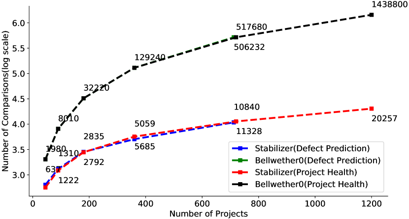
Figure 1. RQ2 results: Number of comparisons.

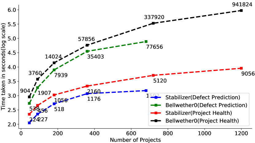
Figure 2. RQ2 results: Median run-time (secs).

5.2. RQ2: Is STABILIZER efficient?

To assess the speed of STABILIZER and compare it against the conventional bellwether, we ran both defect prediction and project health estimation case study on the STABILIZER framework on a sixteen core machine running at 2.3GHz with 32GB of RAM to measure their run time. We also measure the number of comparisons performed in conventional bellwether and our proposed model on both frameworks.

Figure 1 shows the median (over multiple runs) number of comparisons required for finding a bellwether project using conventional bellwether vs STABILIZER for different community sizes ranging from 45 to 1200 projects for both case studies (for defect prediction maximum was 711 projects). The Green and the Black lines show the number of comparisons required for conventional bellwether on the defect prediction and project health estimation case study, respectively. Simultaneously, the Blue and the Red line show the number of comparisons for our STABILIZER algorithm. Here the y-axis is plotted in a log scale while the numbers shown are the actual number of comparisons performed.

Similarly, Figure 2 shows the median run time required for finding a bellwether. We can see from Figure 1 and Figure 2, with increasing community size, the number of comparisons and run-time time increases rapidly for the conventional bellwether method. In contrast, STABILIZER requires a relatively small number of comparisons and run-time (it increases less than linearly).

In summary, STABILIZER will scale to a large space of projects. Its run-time increases less-than-linearly as the project community size increases. STABILIZER is very efficient, requiring less than an hour to terminate for both case studies (756 and 1628 Github projects for defect prediction and project health estimate). Those run-times are 29 to 104 times faster than those seen in Krishna et al.’s BELLWETHER algorithm (the prior SOTA in this area (Krishna and Menzies, 2018)).

5.3. RQ3: Is STABILIZER effective?

The speed improvements reported in RQ2 are only useful if this faster method can also deliver adequate predictions (i.e., predictions that are not worse than those generated by baselines and SOTA).

(a) Defect prediction: Figure 3 shows the performance of all learners from §4.3 on the defect prediction case study. These results are grouped by the “rank” in the left-hand-side column (and this rank was generated using the statistical methods of §4.4).

Looking at our results, in Figure 3, we recommend STABILIZER0; i.e., use the single model found at the root of the STABILIZER tree. We say this since, in all performance measures, STABILIZER0 performs statistically similar or better than our baseline and SOTA methods while also returning the fewest models. To defend this recommendation, we note that:

• We would not recommend Krishna et al.’s Bellwether0 since its run-time is much slower $\Theta(N^{2})$ and that longer run-time is not associated with an outstandingly better performance.

• Nor would we recommend TPTL since it has the outstandingly worst false alarm rate and precision).

• Nor would we recommend STABILIZER1/STABILIZER2 since these never perform statistically different and better than STABILIZER0. Also, they produce more models than STABILIZER0.

• Finally, we see our recommended model STABILIZER0 performs similar to self (which is reference model) in most cases, the only case where self beats STABILIZER0 is recall. This shows that our recommended model performs similarly to the reference model, indicating our transfer learning approach is reaching respectable performance while being able to stable conclusions.

Overall, we summarize Figure 3 results as follows: “Across multiple performance criteria, the faster STABILIZER0 never performs worse than Bellwether0. Furthermore, measured in terms of recall, STABILIZER0 performs statistically better. And thus suitable for transfer learning and generating stable conclusions”.

criteria	rank	treatment	median	IQR
Recall	1	Bellwether0	63	38
	2	TPTL	71	8
	3	STABILIZER0	84	36
	3	STABILIZER1	85	28
	3	global	87	28
	3	STABILIZER2	88	26
	4	self	94	11
False alarm	1	Bellwether0	3	6
	1	STABILIZER0	4	8
	1	self	5	7
	1	STABILIZER1	6	12
	2	STABILIZER2	10	24
	3	global	20	44
	4	TPTL	31	27
Precision	1	TPTL	61	25
	2	global	69	35
	3	STABILIZER2	81	33
	4	STABILIZER1	88	18
	5	STABILIZER0	90	14
	5	self	91	12
	5	Bellwether0	91	13
Popt20	1	TPTL	65	13
	1	global	67	22
	1	self	70	19
	1	STABILIZER2	71	23
	2	STABILIZER1	76	24
	2	STABILIZER0	79	29
	2	Bellwether0	80	20
ifa	1	TPTL	0	1
	1	self	2	5
	1	STABILIZER1	3	6
	1	STABILIZER0	3	5
	1	global	3	10
	1	STABILIZER2	3	7
	1	Bellwether0	3	6

Figure 3. RQ3 results (for defect prediction case study). The “rank” column at left comes from the statistical analysis methods of §4.4. In this study, since we want to minimize false alarm and ifa, then the lowest ranks (i.e., rank=1) are best. But for other measures, which we want to maximize (recall, precision, Popt20), the largest ranks are best.

Goal	Rank	treatment	med	IQR	Goal	Rank	treatment	med	IQR
	1	STABILIZER1	0	0.82		1	self	0.31	0.57
	1	self	0.25	0.7		2	STABILIZER1	0.39	0.79
	1	STABILIZER2	0.25	0.85		2	STABILIZER0	0.46	1
	2	STABILIZER0	0.31	1		2	STABILIZER2	0.53	0.93
	2	Bellwether0	0.79	0.93		2	global	0.7	0.51
MCP	3	global	0.9	0.5	MOP	2	Bellwether0	0.77	0.68
	1	self	0.37	0.44		1	self	0.67	0.57
	2	STABILIZER2	0.52	0.44		2	STABILIZER2	0.76	0.53
	2	STABILIZER1	0.56	0.44		2	STABILIZER1	0.79	1.13
	3	Bellwether0	0.61	0.81		2	global	0.9	0.27
	3	STABILIZER0	0.75	0.82		2	STABILIZER0	0.91	1.58
MCI	3	global	0.75	0.82	MOI	2	Bellwether0	1	0.5
	1	self	0.54	1.09		1	self	0.38	0.41
	1	STABILIZER1	0.6	0.68		2	STABILIZER2	0.56	0.53
	1	STABILIZER2	0.68	0.63		2	STABILIZER1	0.56	0.41
	1	STABILIZER0	1.07	2.04		2	STABILIZER0	0.65	0.48
	1	global	1.16	1.79		2	global	0.65	0.89
MC	2	Bellwether0	8.75	59.48	MS	3	Bellwether0	2.94	5.43
	1	self	0.25	0.43
	2	STABILIZER2	0.38	0.49
	2	STABILIZER1	0.39	0.6
	2	STABILIZER0	0.48	0.51
	2	Bellwether0	0.5	0.74
MAC	2	global	0.62	0.61

Figure 4. RQ3 results (for project health). Same format as Figure 3. For definitions of our goal (MCP, MCI, MC. MAC, MS, MOI, MOP), see Table 3.

(b) Project health estimation: Figure 4 shows the results of the project health estimation case study. Here the performance criterion is MRE, as mentioned in §3.4. Unlike defect prediction case study, project health can be estimated in many ways, as shown in Table 5. For each of the seven goals, the new algorithm STABILIZER is compared against the reference model (i.e. “self”, that uses the local data), global model (“global”), and conventional bellwether (“Bellwether0”)

In all cases of project health estimation goals, our recommended STABILIZER1 did not beat the reference model. Our recommended model reached the reference model performance in two out of seven goals. At the same time, when compared to models that can generate stable conclusions, STABILIZER1 is statistically as good as or better than Bellwether0, global, STABILIZER0 and STABILIZER2. Hence, if the goal is to generate stable conclusions, then the best method seen here (for project health estimation) is STABILIZER1.

5.4. RQ4:Is STABILIZER parsimonious (only generates a few models)?

To answer this question, we count the number of models generated at the best level of STABILIZER’s cluster tree.

According to Figure 3, for defect prediction, the best level is the root of the tree (see the STABILIZER0 results). Since the number of models returned here is one, we can say that, for defect prediction, STABILIZER is very parsimonious.

According to Figure 4, for project health estimation, the best level is the one just down from the root (see the STABILIZER1 results). Figure 4 shows results from seven metrics, and there are some differences in the models generated for each goal. The size of the level1 trees seen in Figure 4 has a mode of nine models:

(MC:8, MOI:8, MAC:9, MOP:9, MCP:9, MCI:9, MS:10)

Note that nine projects are still far less than 1628 used in this study. Hence, we say that STABILIZER for project health is far more parsimonious than using raw project data. That said, STABILIZER for project health is less parsimonious than defect prediction (where only one model is found).

5.5. RQ5:What are the stable conclusions we learned?

In this research question, we explore models which are stable across multiple projects and extract features from models from each case study. We do this to learn what metrics seemed to be most important for prediction and what conclusions can be generated from them? This is done by extracting features which are important for prediction according to the ML model built (i.e., impurity-based feature importance in our case extracted using the scikit-learn API). To determine which features are most important for prediction, we analyze both “locally important” and “globally important” features reported by the respective learners used in this study (Pedregosa et al., 2011a)). Some features are “globally important” since our analysis shows that, across many projects, they are the ones that most predict for defects and estimate for project health. While “locally important” features are feature importance aggregated over all the training projects. We call these features “locally important” since these results come from an analysis that is restricted to just one project at a time.

To show the feature importance of “globally important” and “locally important” features, we use two numbers $x/y$. Here the first number ($x$) is the aggregated feature importance for the best STABILIZER method and the second number ($y$) is feature importance from the local model (self) aggregated over all training projects. Here “globally important” features are those where $x$ is large. Here, (a) if $x/y$ is near one and both $x$ and $y$ are large, then that feature is both “globally” and “locally” important, (b) if $x/y$ is near one and both $x$ and $y$ are small, then that feature is both “globally” and “locally” unimportant, (c) if $x$ ¿ $y$, then that feature is “globally important” but “locally unimportant”, and (d) if $x$ ¡ $y$, then that feature is “locally important” but “globally unimportant”.

5.5.1. Defect Prediction

Table 4 shows the “globally important” features (marked in pink) in the STABILIZER0 defect prediction models. We observe that only three out of 21 features are important in predicting defects. Among these three features, (a) two are experience based metrics; (b) one is change related metric. We analyzed the decisions made by our model to differentiate between a defective and non-defective entry to generate recommendations for the community of 756 Github projects studied here

• The presence of age in the model suggests: review codes which are changed more often. The frequently a file is changed, the more problematic it can become.

• The presence of exp (experience) in our models lets us make the recommendation: minimize the use of amateurs dabbling around the codebase in areas that are unfamiliar to them.

• rexp (recent developer experience) as an important feature suggests: review codes more thoroughly when the changes are made by developers not familiar with the latest changes.

Table 4. Distribution of feature importance using the self model and the STABILIZER0 (Defect Prediction). The pink cells show important features from STABILIZER0. Each cell consists of two numbers(like x/y): the first one (x) is the feature importance for the STABILIZER0 model, and the second one (y) is feature importance for the self model. Learner is Random Forest.

Feature	Feature Importance	Feature	Feature Importance
la	0.0/0.02	avg_nddev	0.07/0.04
ld	0.0/0.05	avg_nadev	0.0/0.03
lt	0.0/0.01	avg_ncomm	0.0/0.01
age	0.22/0.1	ns	0.0/0.0
ddev	0.0/0.09	exp	0.21/0.03
nuc	0.0/0.09	sexp	0.0/0.02
own	0.09/0.07	rexp	0.38/0.07
minor	0.02/0.15	nd	0.0/0.0
ndev	0.0/0.05	sctr	0.0/0.07
ncomm	0.0/0.02	nadev	0.0/0.01
adev	0.0/0.04

Table 5. Distribution of features importance using the self model and the STABILIZER1 model (project health). Each column represents one of the goals mentioned in Table 3. The pink cells show important features from STABILIZER1 derived from the underlying model (i.e., Decision Tree Regressor). Each cell consists of two numbers(like x/y): the first one (x) is for the STABILIZER1 model and the second one (y) is for the self model.

		Target Variables
		MC	MAC	MOP	MCP	MOI	MCI	MS
	MCI	0/0.11	0.02/0.11	0/0.1	0.17/0.13	0/0.07	NA	0/0.08
	MCP	0.46/0.06	0/0.02	0/0.08	NA	0/0.02	0/0.08	0/0.05
	MC	NA	0.14/0.07	0/0.09	0.01/0.09	0/0.09	0/0.05	0/0.1
	MAC	0.28/0.09	NA	0/0.07	0/0.04	0/0.04	0/0.08	0/0.07
	MF	0/0.08	0.61/0.08	0/0.06	0/0.07	0/0.08	0/0.08	0/0.24
	MIC	0/0.1	0.01/0.1	0/0.07	0/0.08	0.22/0.09	1/0.09	0/0.13
	MMP	0.01/0.1	0/0.1	1/0.19	0/0.12	0/0.08	0/0.1	0.13/0.09
	MOI	0/0.07	0.04/0.03	0/0.03	0/0.08	NA	0/0.08	0/0.04
	MOP	0/0.11	0/0.13	NA	0.01/0.16	0/0.06	0/0.09	0.2/0.07
	MPC	0/0.08	0.17/0.08	0/0.11	0.81/0.09	0/0.11	0/0.06	0.67/0.06
	MPM	0.25/0.05	0/0.07	0/0.06	0/0.04	0/0.08	0/0.08	0/0.02
	MS	0/0.07	0/0.09	0/0.08	0/0.07	0.78/0.18	0/0.1	NA
Predictor Variables	MW	0/0.04	0/0.09	0/0.01	0.01/0.02	0/0.07	0/0.09	0/0.03

5.5.2. Project health estimation:

Table 5 shows the features which are “globally important” (marked in pink) for each of the seven project health estimation goals explored in this study. Each row in the table represents a predictor variable (13 variables as suggested by prior work (see § 4.2)), while each column represents one goal (seven goals in total). For each goal, we ask which features in practice are useful when we estimate project health. In this study, using the 1200 projects (from the group of 1628 projects) selected for training, we only find one to three features out of 13 are important.

In summary, we can say:

• MC: for predicting the number of commits in the future, the important features are related to collaboration (MCP, MPM) and activeness (MAC) of the project.

• MAC: for predicting how many active contributors will be there, level of activeness(MC), project popularity (MF), and collaboration (MPC) play an essential role.

• MOP: for estimating how many open PRs will still be active, the level of collaboration is a good indicator.

• MCP: enhancement (MCI) and amount of collaboration (MPC) in a project are good indicators of how many PRs will be closed in the next six months.

• MOI: how many new issues will be in open status in the next six months can be estimated from the amount of enhancement (MIC) and popularity (MS) in a project.

• MCI: the amount of enhancement (MIC) is an accurate indicator for the number of issues closed in the future.

• MS: for estimating the number of stargazers, the amount of collaboration (MMP, MOP, and MPC) is a good indicator.

6. Discussion

In this section we try to discuss what makes our STABILIZER framework unique and why it should be used based on the results of our study and goals set for this research.

Scalable: Unlike the bellwether method proposed by Krishna et al., our STABILIZER framework is scalable. The results from RQ 5.1 shows that STABILIZER framework is order of m times faster than Bellwether0 (aka bellwether method proposed by Krishna et al. (Krishna and Menzies, 2018)) in-case of theoretical average case computational complexity (expressed in-term of $\theta$), where $m$ is the number of clusters formed with $N$ projects. While the results from RQ 5.2 shows that shows that in both case studies STABILIZER framework if much more scalable as number of projects increases, as can be seen in Figure 1 and 2.

Largest Case Study: Exploiting this scalability, we have shown here that STABILIZER with two very large cases studies (one with 756 projects for defect prediction case study and one with 1628 projects for project health estimation case study). In terms of transfer learning lessons learned between multiple projects, this paper is the largest such case study yet reported in the software analytics literature. As stated above in section 1, most prior papers reported their results based on only 20 projects (median value).

Model-agnostic: While version of STABILIZER used here was only tested on random forests, we note that there is nothing in principle preventing the application of this method to a range of other learners. For example, when testing a large number of variants of a deep learner, we would predict that STABILIZER’s divide-and-conqueror (and promote) approach would speed up that analysis.

Performance: We can effectively use the STABILIZER framework if and only if it shows similar or better performance than reference and SOTA methods. In RQ 5.3 we compared our STABILIZER framework with other SOTA and reference models in-term of prediction performance measured with 5 widely used metrics for defect prediction case study and 1 for project health estimation case study. We see that the STABILIZER reaches similar performance to the reference model while performing better then SOTA methods for defect prediction case study, while for project health estimation STABILIZER did not show similar performance to the reference model, but it did out performed other SOTA methods. This result signifies that STABILIZER framework performs significantly better, while being significantly faster.

Conclusion Stability: One goal of this researcher is to find conclusions which are stable across a larger number of projects. If we can’t effectively reduce the number of models generated then we had not solved the problem of conclusion instability. the results from RQ 5.4 shows that can achieve conclusion stability using the STABILIZER framework as the framework found 1 project which can be used as bellwether project for the whole community, signifying the features learned from the model build from that project is stable across 756 projects for the defect prediction case study. While for the project health estimation case study, we find median of 9 projects each specialized for a set of $\approx 200$ projects, signifying features learned from each of these bellwether project’s models is stable across those $\approx 200$ projects. This shows the STABILIZER framework can achieve conclusion stability across a large community of project.

Generally-used Conclusions: Conclusion stability says that new data is not perpetually changing old models. Once that is achieved, the next question to ask is “are those stable conclusions useful?”. RQ 5.5 shows what conclusions can be reached about what features are important in predicting defects and estimating project health in the respective case studies and explains in details whats the importance of each feature in the stable conclusion.

7. Threats to Validity

As with any large-scale empirical study, biases can affect the final results. Therefore, any conclusions made from this work must be considered with the following issues in mind:

(a) Evaluation Bias: While those results are accurate, the conclusion is scoped by the evaluation metrics. It is possible that using other measurements; there may well be a difference in these different kinds of projects. This is a matter that needs to be explored in future research.

(b) Construct Validity: We made many engineering decisions using advice from the literature. That said, we acknowledge that other constructs might lead to different conclusions.

(c) External Validity: The defect prediction dataset was collected using “commit_guru”. It is possible using other tools or methods may result in different outcomes. That said, the “commit_guru” is a tool that is widely used and has detailed documentation.

(d) Statistical Validity: We applied two statistical tests, bootstrap, and the a12. Hence, anytime in this paper, we reported that “X was different from Y” then that report was based on both effect size and statistical significance test.

(e) Sampling Bias: Our conclusions are based on the 756 projects (defect prediction) and 1628 projects (project health estimation). It is possible that different projects would have lead to different conclusions. That said, this sample is very large, so we have some confidence that this sample represents an interesting range of projects.

8. Conclusion

Software engineering suffers from the conclusion instability problem. Ideally, we should be able to generalize to a single model. However, given the diversity of SE, we warn that it is folly to assume that all projects can be represented within a single model.

We presented a method called STABILIZER that recursively replaces many models (clustered into a tree) with one model per sub-tree. That model is then moved up the tree to see if it can replace any higher-level models. Sometimes, this process results in a single model (as in the case of defect prediction). On the other hand, sometimes it does not: for project health estimation, we found that STABILIZER reports nine (median values) models per goal.

It should be emphasized that this approach has only been tested from predictions of defects or project health. However, within that restriction, we say that it is not necessary to always reason about each new project as a new concept that might generate a new model. Even in our worse case (project health), 1628 projects can be represented as nine exemplary models (median value).

Looking forward, based on this conclusion, we make two comments. Firstly, we think this work offers a more rational basis for SE research and SE textbooks. SE is a diverse process, but at least some aspects of that work can be captured in a handful of models. Such a small set of models could be the basis of (e.g.) a 14-week graduate class (one model per week) or a product line of software project tools (one product per model).

Secondly, we warn that much of the prior work on homogeneous transfer learning may have complicated the process with needlessly complicated methods. When building increasingly complex and expensive methods, we strongly recommend that researchers pause and compare their sophisticated methods against simpler alternatives. Going forward from this paper, we would recommend that the transfer learning community uses STABILIZER as a baseline method against which they can test more complex methods.

References

- (1)
- Agrawal and Menzies (2018) Amritanshu Agrawal and Tim Menzies. 2018. ”Better Data” is Better than ”Better Data Miners”(Benefits of Tuning SMOTE for Defect Prediction). ICSE (2018).
- Arar and Ayan (2015) Ömer Faruk Arar and Kürşat Ayan. 2015. Software defect prediction using cost-sensitive neural network. Applied Soft Computing 33 (2015), 263–277.
- Bao et al. (2019) Lingfeng Bao, Xin Xia, David Lo, and Gail C Murphy. 2019. A large scale study of long-time contributor prediction for GitHub projects. IEEE TSE (2019).
- Bidoki et al. (2018) Neda Hajiakhoond Bidoki, Gita Sukthankar, Heather Keathley, and Ivan Garibay. 2018. A Cross-Repository Model for Predicting Popularity in GitHub. In CSCI. IEEE, 1248–1253.
- Bird et al. (2015) Christian Bird, Tim Menzies, and Thomas Zimmermann. 2015. The Art and Science of Analyzing Software Data (1st ed.). Morgan Kaufmann Publishers Inc., San Francisco, CA, USA.
- Bird et al. (2011) Christian Bird, Nachiappan Nagappan, Brendan Murphy, Harald Gall, and Premkumar Devanbu. 2011. Don’t touch my code! Examining the effects of ownership on software quality. In FSE. 4–14.
- Boehm et al. (2000) Barry Boehm, Chris Abts, A Winsor Brown, Sunita Chulani, Bradford K Clark, Ellis Horowitz, Ray Madachy, Donald J Reifer, and Bert Steece. 2000. Cost estimation with COCOMO II. ed: Upper Saddle River, NJ: Prentice-Hall (2000).
- Breiman (2001) Leo Breiman. 2001. Random forests. Machine learning 45, 1 (2001), 5–32.
- Breiman et al. (1984) Leo Breiman, Jerome Friedman, Charles J Stone, and Richard A Olshen. 1984. Classification and regression trees. CRC press.
- Briand et al. (1993) Lionel C Briand, VR Brasili, and Christopher J Hetmanski. 1993. Developing interpretable models with optimized set reduction for identifying high-risk software components. IEEE TSE 19, 11 (1993), 1028–1044.
- Challagulla et al. (2008) Venkata Udaya B Challagulla, Farokh B Bastani, I-Ling Yen, and Raymond A Paul. 2008. Empirical assessment of machine learning based software defect prediction techniques. International Journal on Artificial Intelligence Tools 17, 02 (2008), 389–400.
- Chawla et al. (2002) Nitesh V. Chawla, Kevin W. Bowyer, Lawrence O. Hall, and W. Philip Kegelmeyer. 2002. SMOTE: Synthetic minority over-sampling technique. J. Artif. Intell. Res. 16 (2002). https://doi.org/10.1613/jair.953 arXiv:1106.1813
- Chen et al. (2014) Fangwei Chen, Lei Li, Jing Jiang, and Li Zhang. 2014. Predicting the number of forks for open source software project. In Proceedings of the 2014 3rd International Workshop on Evidential Assessment of Software Technologies. 40–47.
- Cheng et al. (2016) Ming Cheng, Guoqing Wu, Min Jiang, Hongyan Wan, Guoan You, and Mengting Yuan. 2016. Heterogeneous Defect Prediction via Exploiting Correlation Subspace.. In SEKE. 171–176.
- Clark and Madachy (2015) B. Clark and R. Madachy. 2015. Software Cost Estimation Metrics Manual for Defense Systems, Software. Metrics Inc., Haymarket, VA.
- Crowston and Howison (2006) Kevin Crowston and James Howison. 2006. Assessing the health of open source communities. Computer 39, 5 (2006), 89–91.
- Cruz and Ochimizu (2009) Ana Erika Camargo Cruz and Koichiro Ochimizu. 2009. Towards logistic regression models for predicting fault-prone code across software projects. In 2009 3rd international symposium on empirical software engineering and measurement. IEEE, 460–463.
- Devanbu et al. (2016) Premkumar Devanbu, Thomas Zimmermann, and Christian Bird. 2016. Belief & evidence in empirical software engineering. In ICSE. IEEE, 108–119.
- Foundation (2018) Apache Software Foundation. 2018. Apache Software Foundation Projects https://projects.apache.org/projects.html.
- Foundation (2020) Linux Foundation. 2020. Linux Foundation Projects https://www.linuxfoundation.org/projects/directory/.
- Fu et al. (2016a) Wei Fu, Tim Menzies, and Xipeng Shen. 2016a. Tuning for software analytics: Is it really necessary? IST Journal 76 (2016), 135–146.
- Fu et al. (2016b) Wei Fu, Vivek Nair, and Tim Menzies. 2016b. Why is differential evolution better than grid search for tuning defect predictors? arXiv preprint arXiv:1609.02613 (2016).
- Gao et al. (2015) Kehan Gao, Taghi M Khoshgoftaar, and Amri Napolitano. 2015. Combining Feature Subset Selection and Data Sampling for Coping with Highly Imbalanced Software Data.. In SEKE. 439–444.
- Garey and Johnson (1990) Michael R. Garey and David S. Johnson. 1990. Computers and Intractability; A Guide to the Theory of NP-Completeness. W. H. Freeman Co., USA.
- Ghotra et al. (2015) Baljinder Ghotra, Shane McIntosh, and Ahmed E Hassan. 2015. Revisiting the impact of classification techniques on the performance of defect prediction models. In 37th ICSE-Volume 1. IEEE Press, 789–800.
- Hall (1999) Mark Andrew Hall. 1999. Correlation-based feature selection for machine learning. (1999).
- Hamill and Goseva-Popstojanova (2009) M. Hamill and K. Goseva-Popstojanova. 2009. Common trends in software fault and failure data. TSE (2009).
- Hassan (2017) A. Hassan. 2017. Remarks made during a presentation to the UCL Crest Open Workshop.
- He et al. (2014) Peng He, Bing Li, and Yutao Ma. 2014. Towards cross-project defect prediction with imbalanced feature sets. arXiv preprint arXiv:1411.4228 (2014).
- Herbold (2013) Steffen Herbold. 2013. Training data selection for cross-project defect prediction. In Proceedings of the 9th international conference on predictive models in software engineering. 1–10.
- Hosni et al. (2017) Mohamed Hosni, Ali Idri, and Alain Abran. 2017. Investigating heterogeneous ensembles with filter feature selection for software effort estimation. In Proceedings of the 27th International Workshop on Software Measurement and 12th International Conference on Software Process and Product Measurement. 207–220.
- Jansen (2014) Slinger Jansen. 2014. Measuring the health of open source software ecosystems: Beyond the scope of project health. Information and Software Technology 56, 11 (2014), 1508–1519.
- Jarczyk et al. (2018) Oskar Jarczyk, Szymon Jaroszewicz, Adam Wierzbicki, Kamil Pawlak, and Michal Jankowski-Lorek. 2018. Surgical teams on GitHub: Modeling performance of GitHub project development processes. Information and Software Technology 100 (2018), 32–46.
- Jing et al. (2015) Xiaoyuan Jing, Fei Wu, Xiwei Dong, Fumin Qi, and Baowen Xu. 2015. Heterogeneous cross-company defect prediction by unified metric representation and CCA-based transfer learning. In FSE. ACM, 496–507.
- Kalliamvakou et al. (2014) Eirini Kalliamvakou, Georgios Gousios, Kelly Blincoe, Leif Singer, Daniel M. German, and Daniela Damian. 2014. The Promises and Perils of Mining GitHub (MSR 2014). ACM, 10 pages. https://doi.org/10.1145/2597073.2597074
- Khoshgoftaar et al. (2010) Taghi M Khoshgoftaar, Kehan Gao, and Naeem Seliya. 2010. Attribute selection and imbalanced data: Problems in software defect prediction. In Tools with Artificial Intelligence (ICTAI), 2010 22nd IEEE International Conference on, Vol. 1. IEEE.
- Kikas et al. (2016) Riivo Kikas, Marlon Dumas, and Dietmar Pfahl. 2016. Using dynamic and contextual features to predict issue lifetime in GitHub projects. In Proceedings of the 13th International Conference on Mining Software Repositories. ACM, 291–302.
- Kim et al. (2011) Miryung Kim, Dongxiang Cai, and Sunghun Kim. 2011. An empirical investigation into the role of API-level refactorings during software evolution. In Proceedings of the 33rd ICSE. ACM, 151–160.
- Kim et al. (2016) Miryung Kim, Thomas Zimmermann, Robert DeLine, and Andrew Begel. 2016. The Emerging Role of Data Scientists on Software Development Teams. In Proceedings of the 38th ICSE (Austin, Texas) (ICSE ’16). ACM, New York, NY, USA, 96–107. https://doi.org/10.1145/2884781.2884783
- Kocaguneli et al. (2015) Ekrem Kocaguneli, Tim Menzies, and Emilia Mendes. 2015. Transfer Learning in Effort Estimation. Empirical Softw. Engg. 20, 3 (June 2015), 813–843. https://doi.org/10.1007/s10664-014-9300-5
- Koru et al. (2009) A G. Koru, D. Zhang, K. El Emam, and H. Liu. 2009. An investigation into the functional form of the size-defect relationship for software modules. TSE (2009).
- Krishna and Menzies (2017) Rahul Krishna and Tim Menzies. 2017. Simpler Transfer Learning (Using” Bellwethers”). arXiv preprint arXiv:1703.06218. Under review, IEEE TSE (2017).
- Krishna and Menzies (2018) Rahul Krishna and Tim Menzies. 2018. Bellwethers: A Baseline Method For Transfer Learning. IEEE TSE (2018).
- Krishna et al. (2016a) Rahul Krishna, Tim Menzies, and Wei Fu. 2016a. Too Much Automation? The Bellwether Effect and Its Implications for Transfer Learning. In ASE’16.
- Krishna et al. (2016b) Rahul Krishna, Tim Menzies, and Wei Fu. 2016b. Too much automation? the bellwether effect and its implications for transfer learning. In ASE. ACM Press, New York, New York, USA. https://doi.org/10.1145/2970276.2970339
- Lee et al. (2016) Taek Lee, Jaechang Nam, Donggyun Han, Sunghun Kim, and Hoh Peter In. 2016. Developer micro interaction metrics for software defect prediction. IEEE TSE 42, 11 (2016), 1015–1035.
- Link and Germonprez (2018) Georg JP Link and Matt Germonprez. 2018. Assessing open source project health. (2018).
- Liu et al. (2019) Chao Liu, Dan Yang, Xin Xia, Meng Yan, and Xiaohong Zhang. 2019. A two-phase transfer learning model for cross-project defect prediction. Information and Software Technology 107 (2019), 125–136.
- Ma et al. (2012a) Ying Ma, Guangchun Luo, Xue Zeng, and Aiguo Chen. 2012a. Transfer learning for cross-company software defect prediction. Information and Software Technology 54, 3 (2012), 248–256.
- Ma et al. (2012b) Ying Ma, Guangchun Luo, Xue Zeng, and Aiguo Chen. 2012b. Transfer learning for cross-company software defect prediction. Information and Software Technology 54, 3 (2012), 248–256. https://doi.org/10.1016/j.infsof.2011.09.007
- Manikas and Hansen (2013) Konstantinos Manikas and Klaus Marius Hansen. 2013. Reviewing the health of software ecosystems-a conceptual framework proposal. In Proceedings of the 5th international workshop on software ecosystems (IWSECO). Citeseer, 33–44.
- Mantyla et al. (2004) Mika V Mantyla, Jari Vanhanen, and Casper Lassenius. 2004. Bad smells-humans as code critics. In 20th IEEE International Conference on Software Maintenance, 2004. Proceedings. IEEE, 399–408.
- Matsumoto et al. (2010) S. Matsumoto, Y. Kamei, A. Monden, K. Matsumoto, and M. Nakamura. 2010. An analysis of developer metrics for fault prediction. In 6th PROMISE.
- Mensah et al. (2017a) Solomon Mensah, Jacky Keung, Michael Franklin Bosu, Kwabena Ebo Bennin, and Patrick Kwaku Kudjo. 2017a. A Stratification and Sampling Model for Bellwether Moving Window.. In SEKE. 481–486.
- Mensah et al. (2017b) Solomon Mensah, Jacky Keung, Stephen G MacDonell, Michael F Bosu, and Kwabena E Bennin. 2017b. Investigating the significance of bellwether effect to improve software effort estimation. In Software Quality, Reliability and Security (QRS), 2017 IEEE International Conference on. IEEE, 340–351.
- Mensah et al. (2018) S. Mensah, J. Keung, S. G. MacDonell, M. F. Bosu, and K. E. Bennin. 2018. Investigating the Significance of the Bellwether Effect to Improve Software Effort Prediction: Further Empirical Study. IEEE Transactions on Reliability 67, 3 (Sept 2018), 1176–1198. https://doi.org/10.1109/TR.2018.2839718
- Menzies et al. (2013) Tim Menzies, Andrew Butcher, David Cok, Andrian Marcus, Lucas Layman, Forrest Shull, Burak Turhan, and Thomas Zimmermann. 2013. Local versus global lessons for defect prediction and effort estimation. IEEE TSE 39, 6 (2013), 822–834.
- Menzies et al. (2011) Tim Menzies, Andrew Butcher, Andrian Marcus, Thomas Zimmermann, and David Cok. 2011. Local vs. global models for effort estimation and defect prediction. In 2011 26th IEEE/ACM International Conference on Automated Software Engineering (ASE 2011). IEEE, 343–351.
- Minku et al. (2015) Leandro Minku, Federica Sarro, Emilia Mendes, and Filomena Ferrucci. 2015. How to make best use of cross-company data for web effort estimation?. In 2015 ACM/IEEE International Symposium on Empirical Software Engineering and Measurement (ESEM). IEEE, 1–10.
- Misirli et al. (2011) A. T. Misirli, A. Bener, and R. Kale. 2011. Ai-based software defect predictors: Applications and benefits in a case study. AI Magazine (2011).
- Mittas and Angelis (2013) Nikolaos Mittas and Lefteris Angelis. 2013. Ranking and clustering software cost estimation models through a multiple comparisons algorithm. IEEE TSE 39, 4 (2013), 537–551.
- Munaiah et al. (2017) Nuthan Munaiah, Steven Kroh, Craig Cabrey, and Meiyappan Nagappan. 2017. Curating GitHub for engineered software projects. Empirical Software Engineering 22, 6 (01 Dec 2017), 3219–3253. https://doi.org/10.1007/s10664-017-9512-6
- Nagappan et al. (2010) Nachiappan Nagappan, Andreas Zeller, Thomas Zimmermann, Kim Herzig, and Brendan Murphy. 2010. Change bursts as defect predictors. In 2010 IEEE 21st international symposium on software reliability engineering. IEEE, 309–318.
- Nam et al. (2017) Jaechang Nam, Wei Fu, Sunghun Kim, Tim Menzies, and Lin Tan. 2017. Heterogeneous defect prediction. IEEE TSE (2017).
- Nam and Kim (2015) Jaechang Nam and Sunghun Kim. 2015. Heterogeneous defect prediction. In Proc. 2015 10th Jt. Meet. Found. Softw. Eng. - ESEC/FSE 2015. ACM Press, New York, New York, USA, 508–519. https://doi.org/10.1145/2786805.2786814
- Nam et al. (2013) Jaechang Nam, Sinno Jialin Pan, and Sunghun Kim. 2013. Transfer defect learning. In Proceedings - ICSE. 382–391.
- Onan et al. (2016) Aytuğ Onan, Serdar Korukoğlu, and Hasan Bulut. 2016. A multiobjective weighted voting ensemble classifier based on differential evolution algorithm for text sentiment classification. Expert Systems with Applications 62 (2016).
- Ostrand et al. (2004) Thomas J Ostrand, Elaine J Weyuker, and Robert M Bell. 2004. Where the bugs are. ACM SIGSOFT Software Engineering Notes 29, 4 (2004), 86–96.
- Pan and Yang (2009) Sinno Jialin Pan and Qiang Yang. 2009. A survey on transfer learning. IEEE Transactions on knowledge and data engineering 22, 10 (2009), 1345–1359.
- Pedregosa et al. (2011a) Fabian Pedregosa, Gaël Varoquaux, Alexandre Gramfort, Vincent Michel, Bertrand Thirion, Olivier Grisel, Mathieu Blondel, Peter Prettenhofer, Ron Weiss, Vincent Dubourg, et al. 2011a. Scikit-learn: Machine learning in Python. the Journal of machine Learning research 12 (2011).
- Pedregosa et al. (2011b) F. Pedregosa, G. Varoquaux, A. Gramfort, V. Michel, B. Thirion, O. Grisel, M. Blondel, P. Prettenhofer, R. Weiss, V. Dubourg, J. Vanderplas, A. Passos, D. Cournapeau, M. Brucher, M. Perrot, and E. Duchesnay. 2011b. Scikit-learn: Machine Learning in Python. Journal of Machine Learning Research 12 (2011), 2825–2830.
- Pelayo and Dick (2007) Lourdes Pelayo and Scott Dick. 2007. Applying Novel Resampling Strategies To Software Defect Prediction. In NAFIPS 2007 - 2007 Annu. Meet. North Am. Fuzzy Inf. Process. Soc. IEEE, 69–72. https://doi.org/10.1109/NAFIPS.2007.383813
- Rahman and Devanbu (2013) Foyzur Rahman and Premkumar Devanbu. 2013. How, and Why, Process Metrics Are Better. In Proceedings of the 2013 ICSE (San Francisco, CA, USA) (ICSE ’13). IEEE Press, 432–441.
- Rodriguez et al. (2007) Daniel Rodriguez, Roberto Ruiz, J Cuadrado-Gallego, J Aguilar-Ruiz, and Miguel Garre. 2007. Attribute selection in software engineering datasets for detecting fault modules. In 33rd EUROMICRO Conference on Software Engineering and Advanced Applications (EUROMICRO 2007). IEEE.
- Rosen et al. (2015) Christoffer Rosen, Ben Grawi, and Emad Shihab. 2015. Commit guru: analytics and risk prediction of software commits. In Proceedings of the 2015 10th Joint Meeting on Foundations of Software Engineering. ACM, 966–969.
- Saeys et al. (2008) Yvan Saeys, Thomas Abeel, and Yves Van de Peer. 2008. Robust feature selection using ensemble feature selection techniques. In Joint European Conference on Machine Learning and Knowledge Discovery in Databases. Springer, 313–325.
- Sarro et al. (2016) Federica Sarro, Alessio Petrozziello, and Mark Harman. 2016. Multi-objective software effort estimation. In Proceedings of the 38th ICSE. ACM, 619–630.
- Sawyer (2013) Robert Sawyer. 2013. BI’s Impact on Analyses and Decision Making Depends on the Development of Less Complex Applications. In Principles and Applications of Business Intelligence Research. IGI Global, 83–95.
- Sayyad et al. (2013a) Abdel Salam Sayyad, Joseph Ingram, Tim Menzies, and Hany Ammar. 2013a. Scalable Product Line Configuration: A Straw to Break the Camel’s Back. In ASE (ASE’13). IEEE Press, 465–474. https://doi.org/10.1109/ASE.2013.6693104
- Sayyad et al. (2013b) Abdel Salam Sayyad, Tim Menzies, and Hany Ammar. 2013b. On the Value of User Preferences in Search-based Software Engineering: A Case Study in Software Product Lines. In Proceedings of the 2013 ICSE (ICSE ’13). 492–501.
- Shepperd and MacDonell (2012) Martin Shepperd and Steve MacDonell. 2012. Evaluating prediction systems in software project estimation. Information and Software Technology 54, 8 (2012), 820–827.
- Shrikanth and Menzies (2019) NC Shrikanth and Tim Menzies. 2019. Assessing Practitioner Beliefs about Software Defect Prediction. arXiv (2019), arXiv–1912.
- Sjøberg et al. (2012) Dag IK Sjøberg, Aiko Yamashita, Bente CD Anda, Audris Mockus, and Tore Dybå. 2012. Quantifying the effect of code smells on maintenance effort. IEEE TSE 39, 8 (2012), 1144–1156.
- Storn and Price (1997) R. Storn and K. Price. 1997. Differential evolution–a simple and efficient heuristic for global optimization over cont. spaces. JoGO 11, 4 (1997), 341–359.
- Sun et al. (2012) Zhongbin Sun, Qinbao Song, and Xiaoyan Zhu. 2012. Using coding-based ensemble learning to improve software defect prediction. IEEE Transactions on Systems, Man, and Cybernetics, Part C (Applications and Reviews) 42, 6 (2012), 1806–1817.
- Tan et al. (2015) Ming Tan, Lin Tan, Sashank Dara, and Caleb Mayeux. 2015. Online defect prediction for imbalanced data. In 2015 IEEE/ACM 37th IEEE ICSE, Vol. 2. IEEE.
- Tan and Chan (2016) Shiang-Yen Tan and Taizan Chan. 2016. Defining and conceptualizing actionable insight: a conceptual framework for decision-centric analytics. arXiv preprint arXiv:1606.03510 (2016).
- Tantithamthavorn et al. (2018) Chakkrit Tantithamthavorn, Shane McIntosh, Ahmed E Hassan, and Kenichi Matsumoto. 2018. The impact of automated parameter optimization on defect prediction models. IEEE TSE 45, 7 (2018), 683–711.
- Tufano et al. (2015) Michele Tufano, Fabio Palomba, Gabriele Bavota, Rocco Oliveto, Massimiliano Di Penta, Andrea De Lucia, and Denys Poshyvanyk. 2015. When and why your code starts to smell bad. In 2015 IEEE/ACM 37th IEEE ICSE, Vol. 1. IEEE, 403–414.
- Turhan et al. (2009a) Burak Turhan, Tim Menzies, Ayşe B Bener, and Justin Di Stefano. 2009a. On the relative value of cross-company and within-company data for defect prediction. Empirical Software Engineering 14, 5 (2009), 540–578.
- Turhan et al. (2009b) Burak Turhan, Tim Menzies, Ayşe B Bener, and Justin Di Stefano. 2009b. On the relative value of cross-company and within-company data for defect prediction. Empirical Software Engineering 14, 5 (2009), 540–578.
- Uddin and Uddiny (2015) Md Taufeeq Uddin and Md Azher Uddiny. 2015. A guided random forest based feature selection approach for activity recognition. In ICEEICT. IEEE, 1–6.
- Wahyudin et al. (2007) Dindin Wahyudin, Khabib Mustofa, Alexander Schatten, Stefan Biffl, and A Min Tjoa. 2007. Monitoring the “health” status of open source web-engineering projects. International Journal of Web Information Systems (2007).
- Wan et al. (2018) Zhiyuan Wan, Xin Xia, Ahmed E Hassan, David Lo, Jianwei Yin, and Xiaohu Yang. 2018. Perceptions, expectations, and challenges in defect prediction. IEEE TSE (2018).
- Wang and Yao (2013) Shuo Wang and Xin Yao. 2013. Using class imbalance learning for software defect prediction. IEEE Transactions on Reliability 62, 2 (2013), 434–443.
- Wang et al. (2018) Tao Wang, Yang Zhang, Gang Yin, Yue Yu, and Huaimin Wang. 2018. Who Will Become a Long-Term Contributor? A Prediction Model based on the Early Phase Behaviors. In Proceedings of the Tenth Asia-Pacific Symposium on Internetware. 1–10.
- Wynn Jr (2007) Donald Wynn Jr. 2007. Assessing the health of an open source ecosystem. In Emerging Free and Open Source Software Practices. IGI Global, 238–258.
- Xia (2021) Tianpei Xia. 2021. Principles of Project health for Open Source Software.
- Xia et al. (2020) Tianpei Xia, Wei Fu, Rui Shu, and Tim Menzies. 2020. Predicting Project Health for Open Source Projects (using the DECART Hyperparameter Optimizer). arXiv preprint arXiv:2006.07240 (2020).
- Xu et al. (2019) Zhou Xu, Shuai Pang, Tao Zhang, Xia-Pu Luo, Jin Liu, Yu-Tian Tang, Xiao Yu, and Lei Xue. 2019. Cross project defect prediction via balanced distribution adaptation based transfer learning. Journal of Computer Science and Technology 34, 5 (2019), 1039–1062.
- Yang et al. (2017) Xinli Yang, David Lo, Xin Xia, and Jianling Sun. 2017. TLEL: A two-layer ensemble learning approach for just-in-time defect prediction. Information and Software Technology 87 (2017), 206–220.
- Yu et al. (2017) Qiao Yu, Shujuan Jiang, and Yanmei Zhang. 2017. A feature matching and transfer approach for cross-company defect prediction. Journal of Systems and Software 132 (2017), 366–378.
- Zhang et al. (2018) Chong Zhang, Kay Chen Tan, Haizhou Li, and Geok Soon Hong. 2018. A cost-sensitive deep belief network for imbalanced classification. IEEE transactions on neural networks and learning systems 30, 1 (2018), 109–122.
- Zhang et al. (2016) Feng Zhang, Audris Mockus, Iman Keivanloo, and Ying Zou. 2016. Towards building a universal defect prediction model with rank transformed predictors. Empirical Software Engineering 21, 5 (2016), 2107–2145.
- Zhang et al. (1996) Tian Zhang, Raghu Ramakrishnan, and Miron Livny. 1996. BIRCH: an efficient data clustering method for very large databases. In ACM Sigmod Record, Vol. 25. ACM, 103–114.
- Zhou et al. (2010) Yuming Zhou, Baowen Xu, and Hareton Leung. 2010. On the ability of complexity metrics to predict fault-prone classes in object-oriented systems. Journal of Systems and Software 83, 4 (2010), 660–674.
- Zimmermann et al. (2009) Thomas Zimmermann, Nachiappan Nagappan, Harald Gall, Emanuel Giger, and Brendan Murphy. 2009. Cross-project defect prediction: a large scale experiment on data vs. domain vs. process. In FSE. 91–100.
- Zimmermann et al. (2007) Thomas Zimmermann, Rahul Premraj, and Andreas Zeller. 2007. Predicting defects for eclipse. In Proceedings of the Third International Workshop on Predictor Models in Software Engineering. IEEE Computer Society, 9.
- Zitzler et al. (2002) Eckart Zitzler, Marco Laumanns, and Lothar Thiele. 2002. SPEA2: Improving the Strength Pareto Evolutionary Algorithm for Multiobjective Optimization. In Evolutionary Methods for Design, Optimisation, and Control. CIMNE, Barcelona, Spain, 95–100.