Negativity-Mutual Information conversion and coherence in two-coupled harmonic oscillators

Abstract

Quantum information is a common topic of research in many areas of quantum physics, such as quantum communication and quantum computation, as well as quantum thermodynamics. It can be encoded in discrete or continuous variable systems, with the appropriated formalism to treat it generally depending on the quantum system to be chosen. For continuous variable systems, it is convenient to employ a quasi-probability function to represent quantum states and non-classical signatures. The Wigner function is a special quasi-probability function because it allows to describe a quantum system in the phase space very similar to the classical one. In this work we consider some informational aspects of two-mode continuous variables systems. In particular we illustrate how the mutual information may be useful to transfer the non-Gaussianity property between two states. Moreover, the coherence of a Gaussian state is studied when the system is coupled to a thermal reservoir but also with an extra single-mode Gaussian state. Our results may be, in principle, investigated in trapped ions setups, where the two-mode system can be encoded in the vibrational modes of the ion.

I Introduction

The complete ability of quantification and manipulation of quantum information is a paramount challenge to design new micro and nano devices based on quantum properties of systems. It is expected that this fine control would have important impacts on quantum communication and quantum cryptography Pleni02 ; Weekbrook2014 ; Pirandola2017 ; Pirandola2015 , quantum metrology Cirac2019 ; Adesso2017 , quantum thermodynamics Camati2019 ; Kosloff2019 ; Shanhe2019 , and quantum computation Zureck01 ; Supre2019 ; Silva2015 . These current and future implications emphasize the importance in understanding quantum information in as many points of view as possible, mainly because different experimental platforms require an appropriated set of tools to manipulate information. Encoding and processing information depend on the quantum system to be considered. There are basically two broad classes of quantum systems for these purposes, the two-level and continuous variable systems. The first of them has a large numbers of studies, ranging from the use of quantum information to reverse the direction of heat in quantum thermodynamics Partovi2008 ; Jevtic2012 ; Serra2019 , to investigate backflow of information in non-Markovian dynamics Maniscalco2018 ; Maniscalco2017 ; Camati2020 . The latter, despite of some relevant works as, for instance, in squeezed states Feig2019 ; Giovannetti01 ; Serafini2018 and in photon addition and subtraction Su2019 , possesses relevant points to be addressed, as the quality of squeezing sources and detectors, and quantum computation architecture Adesso ; Weedbrook2012 .

In what concerns the case of quantum information in two-level systems, it is considered that the most adequate formalism is the wave function or, in general cases, the density operator approach Petruccione01 ; Nielsen . On the other hand, for continuous variable quantum systems, such as in quantum optics Quantumopticsbook , trapped ions Wineland2003 ; Sage2019 , cold atoms Biedermann2015 and cavity QED Han2018 ; Werlang2018 , it is common to employ, besides the density operator, a quasi-probability function to represent the state of some system Zachosbook . When dealing with the quantum to classical transition, the most suitable of these functions is the Wigner function Wigner1932 ; Case2008 , which is represented in a phase space similarly to that of the classical physics. The Wigner function has given important contribution in quantum physics, for instance, in implementing teleportation of a quantum gate Chou2018 and in general uncertainty relations in quantum systems Santos2015 ; Santos2016 ; Bernardini01 . However, in many cases it has been used more as a mean of visualization than to properly describe the state of the system. There exist, nonetheless, the so-called phase-space formalism of quantum mechanics, in which the Wigner function is the state of some system and all the observables are complex functions represented in the phase space.

The core of the phase-space formalism of quantum mechanics is the Weyl tranform Case2008 ; Rosenbaum2006 , which converts a given operator in a complex function. The Wigner function is then defined as the Weyl transform of the density operator, for pure or mixed states. The Moyal product Zachosbook is also an important ingredient, once it provides the appropriated inner product, in order to guarantee the uncertainty relations of the quantum theory. Based on these main elements, a formalism to treat quantum information, non-classicality signatures, and coherence can be established. In this work, we study some properties of two-mode continuous variables systems from the point of view of quantum information. In particular, we investigated the mutual information between two systems and show that it can be employed to transfer the negativity of a number state to a Gaussian one in a unitary dynamics. Moreover, we quantify the coherence of a Gaussian state when the system is in contact with a thermal reservoir but also with another harmonic oscillator. We verify the increase of the coherence in some time interval during the dynamics and that this effect is in accordance with a non-trivial behavior of the fidelity.

We note that these effects could be, in principle, experimentally performed in trapped ions setups, where the two-mode system is encoded in the vibrational models of the ions Twamley1997 ; Wineland1996 ; Zhong2018 ; Ortiz2017 . On the other hand, the negativity of CV states are important in quantum information, where they can be employed as resources in different protocols Paris2018 .

This manuscript is organized as follows. In section II we provide the basic properties of the Wigner function and the phase-space formalism of quantum mechanics. In section III we consider a two-mode state evolving unitarily in order to show that the mutual information allows the transference of the negativity of a number state to a Gaussian one. Section IV is devoted to study the dissipative dynamics of a one-mode Gaussian state interacting with a thermal reservoir as well as with another harmonic oscillator, from the point of view of the coherence during the dynamics. Here it is shown that the fidelity works as a witness of non-Markovian like-effect. We briefly discuss a trapped ions approach that could be useful to implement our findings in Section V. Finally, we draw our conclusions and final remarks in section VI.

II Theoretical framework

In this section we review some relevant properties of the Wigner function and the phase-space formalism of quantum mechanics. The standard formalism of quantum mechanics is based on operators that act on the Hilbert space, $\mathcal{H}$. A quantum system can be described by means of a wave function in the position representation or, through the Fourier transform, in the momentum representation. Moreover, there is the well-known commutation relation between position and momentum operators, $[\hat{q}_{i},\hat{p}_{j}]=i\hbar\delta_{ij}$, where $i$ and $j$ run over all the Hilbert space.

The operators-based formalism is not the only way to describe quantum mechanics. The phase-space formalism of quantum mechanics (PSQM) is another interesting way to study quantum mechanical systems, being relevant in a large number of scenarios. In the PSQM, the Wigner function represents the state of a given system and has the important property of carrying out simultaneously information about position and momentum of the system. In order to introduce the Wigner function and the phase-space formalism, we consider the Weyl transform of an operator $\hat{\mathcal{O}}(\hat{q},\hat{p})$, defined as Zachosbook ; Case2008 ,

$$A^{W}(q,p)=\int dy\,e^{-ipy/\hbar}\langle q+y/2|\hat{\mathcal{O}}(\hat{q},\hat{p})|q-y/2\rangle,$$ (1)

where $W$ stands for Weyl transform. The Weyl transform converts an operator in a c-function and it is a natural connection between operators-based and phase-space formalisms.

Next, considering a system described by a pure state, $|\psi\rangle$, we can write the density operator, $\hat{\rho}=|\psi\rangle\langle\psi|$. The Wigner function can be defined just as the Weyl tranform of the density operator,

$$W(q,p) =h^{-1}\int dy\,e^{-ipy/\hbar}\langle q+y/2|\hat{\mathcal{\rho}}|q-y/2\rangle,$$

$$=h^{-1}\int dy\,e^{-ipy/\hbar}|\psi(q+y/2)\rangle\langle\psi(q-y/2)|.$$ (2)

Some important properties of the Wigner function are that it is normalized when integrated over all phase-space, additionally providing the marginal probability distribution for momentum $|\phi(p)|^{2}$, and position $|\psi(q)|^{2}$,

$$\int dq\,W(q,p)=|\phi(p)|^{2},\quad\int dp\,W(q,p)=|\psi(q)|^{2}.$$ (3)

From the Wigner function, it is also possible to obtain the expectation the value of an observable $\mathcal{O}$,

$$\langle\mathcal{O}\rangle=h^{-1}\int\int dqdp\,W(q,p)\mathcal{O}^{W}(q,p).$$ (4)

The generalization of the Wigner function for mixed states is straightforward. For a mixed state $\rho=\sum_{j}p_{j}|\psi_{j}\rangle\langle\psi_{j}|$, where $p_{j}$ is the probability of each state and it is always positive, with $\sum_{j}p_{j}=1$, the Wigner function is simply given by,

$$W(q,p)=\sum_{j}p_{j}W_{j}(q,p),$$ (5)

with $W_{j}(q,p)$ the Wigner function associated to each part of the ensemble.

One of the basic ingredients in considering the PSQM formalism is the Moyal product, which is introduced once we are now dealing with c-functions and no longer with operators. The Moyal product, defined for position and momentum variables Zachosbook , reads $\mathcal{A}^{W}(q,p)\star\mathcal{B}^{W}(q,p),$ where,

$$\star=\text{exp}\left[\frac{i\hbar}{2}\left(\frac{\overleftarrow{\partial}}{\partial q}\frac{\overrightarrow{\partial}}{\partial p}-\frac{\overleftarrow{\partial}}{\partial p}\frac{\overrightarrow{\partial}}{\partial q}\right)\right].$$ (6)

In introducing the Moyal product into the PSQM formalism we obtain a set of important tools to treat quantum systems, most of them being very similar to the classical case. In particular, for a unitary dynamics, the time evolution of an observable $\mathcal{O}^{W}$is dictated by the equation,

$$\dot{\mathcal{O}}^{W}(q,p;t) =-\frac{i}{\hbar}\left[\mathcal{O}^{W}(q,p;0),H^{W}(q,p;t)\right]_{\star}$$

$$=\frac{i}{\hbar}\mathcal{O}^{W}(q,p;0)\star H^{W}(q,p;t)$$ (7)

$$-\frac{i}{\hbar}H^{W}(q,p;t)\star\mathcal{O}^{W}(q,p;0),$$ (8)

well known as Moyal equation. For a generalization of the Moyal equation for open quantum systems we refer to Ref. Deering2015 .

In addition, applying the Weyl tranform on the eigenvalue equation and using the Moyal product, we obtain the so-called stargenvalue equation, given by Zachosbook ; Rosenbaum2006 ,

$$H^{W}(q,p)\star W(q,p)=EW(q,p),$$ (9)

where $H^{W}(q,p)$ is the Weyl tranform of the Hamiltonian of a quantum system and $E$ sets for the eigenvalues of energy. In the case of a quantum system with $N$ dimensions, the selection of a particular sub phase space $(q_{k},p_{k})$ is performed by integrating over the rest of the variables,

$$W(q_{k},p_{k})=\int\int dq_{N-k}dp_{N-k}\,W(q_{\ell},p_{\ell}).$$ (10)

Additionally, we present how to obtain the time evolution of the Wigner function using the Moyal product in the case of a unitary operation. Once the initial Wigner function is obtained from Eq. (9), the time evolution is given by the unitary operator Zachosbook ,

$$U_{\star}(q_{\ell},p_{\ell};t) =e^{itH^{W}/\hbar}=1+(it/\hbar)H^{W}$$ (11)

$$+\frac{(it/\hbar)^{2}}{2!}H^{W}\star H^{W}+...,$$ (12)

with $\ell=1,...,N,$and $N$ the dimension of the system, resulting in,

$$W(q_{\ell},p_{\ell};t)=U_{\star}^{-1}(q_{\ell},p_{\ell};t)\star W(q_{\ell},p_{\ell};0)\star U_{\star}(q_{\ell},p_{\ell};t).$$ (13)

Finally, for the case in which the system is a two-mode Gaussian state, we can introduce a vector collecting all the coordinates of the phase space, $\vec{R}(q_{1},p_{1},q_{2},p_{2})$. The two-mode Gaussian state is then completely characterized in terms of its first moments and the covariance matrix, defined as $\vec{d}=(\langle q_{1}\rangle,\langle p_{1}\rangle,\langle q_{2}\rangle,\langle p_{2}\rangle)$ and $\sigma=\sigma_{11}\oplus\sigma_{22}$ , respectively, with,

$$\sigma_{ii}=\left(\begin{array}[]{cc}\sigma_{q_{i}q_{i}}&\sigma_{p_{i}q_{i}}\\ \sigma_{q_{i}p_{i}}&\sigma_{p_{i}p_{i}}\end{array}\right),$$ (14)

and $\sigma_{AB}=\langle AB+BA\rangle-2\langle A\rangle\langle B\rangle$. This results in a convenient expression for obtaining the Wigner function Adesso ; Weedbrook2012 ,

$$W_{G}(\vec{R})=\frac{exp\left[-(1/2)(\vec{R}-\vec{d})\sigma^{-1}(\vec{R}-\vec{d})\right]}{(2\pi)^{4}\sqrt{Det[\sigma]}},$$ (15)

particularizing the expression for two modes.

Now, we present some informational quantifiers which will be relevant for our discussion. The first point to be addressed is the introduction of linear entropy. The treatment will be restricted for a bipartite system. Since a direct translation of the von Neumann entropy to the phase-space is not generally possible because the Wigner function may assume negative values, the main alternative adopted is to employ the well-known linear entropy, defined as Mandredi2000 ,

$$S=1-(2\pi\hbar)^{2}\int\int dq_{i}dp_{i}\,W^{2}(q_{i},p_{i}),$$ (16)

with $i=1,2$.

The Eq. (16) holds for pure and mixed quantum states and satisfies the relation $0\leq S\leq 1$, where $S=0$ for a pure state.

Mutual information. The linear entropy is useful to define the mutual information between two parts of a bipartite quantum system. Let consider a quantum system described by a Wigner function $W(q_{i},p_{i})$ where the parts may have some physical interaction. The mutual information shared between the two parts is defined as Santos2015 ; Bernardini01 ; Mandredi2000 ,

$$I^{(1:2)}=S(W_{1})+S(W_{2})-S(W),$$ (17)

where $W_{1}$ and $W_{2}$ are the local Wigner functions of each part,

$$W_{1} =W(q_{1},p_{1})=\int\int dq_{2}dp_{2}\,W(q_{i},p_{i}),$$

$$W_{2} =W(q_{2},p_{2})=\int\int dq_{1}dp_{1}\,W(q_{i},p_{i}).$$

The mutual information measures the total correlation, classical or quantum, between two parts of a system. When the bipartite system is separable, $W(q_{i},p_{i})=W(q_{1},p_{1})W(q_{2},p_{2})$, the mutual information is zero.

Wigner function negativity. Another way of quantifying non-classical effects in a system is the negativity of the local Wigner function, defined in a bipartite system as Kenfack2014 ,

$$\delta(W_{1}) =\int\int dq_{1}dp_{1}\,|W_{1}|-\int\int dq_{1}dp_{1}\,W_{1},$$

$$\delta(W_{2}) =\int\int dq_{2}dp_{2}\,|W_{2}|-\int\int dq_{2}dp_{2}\,W_{2}.$$

The negativity of the Wigner function has been used in different cases for investigating non-classical effects Rundle2017 ; Treps2017 ; Svozil=0000EDk2018 and reported experimentally in Ref. Haroche2000 , with applications in quantum computation Okay2014 . For separable or correlated bipartite states the negativity is directly related to non-classical effects of each part. Thus, using the mutual information and the negativity it is possible to have a broad knowledge on the correlations shared between the two parts of a system.

Particular case: Gaussian states

Here we detail some quantum information quantities in the particular case in which the Wigner function is Gaussian, i.e. completely characterized by the first and second moments Adesso ; Serafini ; Hiroshima2007 ; Weedbrook2012 .

Fidelity. The fidelity is a suitable way of comparing how similar (or distinct) two states are. Consider two Gaussian states, characterized by their first and seconds moments (covariance matrix), $\vec{d}$ and $\sigma$, respectively, such that we can write the states as $W_{1}(\vec{d}_{1},\sigma_{1})$ and $W_{2}(\vec{d}_{2},\sigma_{2})$. The fidelity is given by Holevo ; Scutaru ,

$$F(\sigma_{1},\vec{d}_{1};\sigma_{2},\vec{d}_{2})=\frac{2}{\sqrt{\Delta+\delta}-\sqrt{\delta}}e^{-\frac{1}{2}\vec{d}^{T}\sigma_{+}^{-1}\vec{d}},$$ (18)

where $\Delta\equiv Det[\sigma_{1}+\sigma_{2}]$, $\delta=(Det[\sigma_{1}]-1)(Det[\sigma_{2}]-1)$, $\vec{d}\equiv\vec{d}_{1}-\vec{d}_{2}$, and $\sigma_{+}=\sigma+\sigma_{2}$. The fidelity is bounded by $0\leq F\leq 1$, with $F=1$ and $F=0$ for identical and completely different states, respectively. Equation (18) has particular importance in quantum information processing with Gaussian states because it allows, for example, to quantify the quality of a given noisy communication channel, where we have Gaussian states as input and output Hiroshima2007 . Another important point is that the covariance matrix is experimentally accessible, in particular in quantum optical devices Hage2007 .

Coherence. An important quantum signature is the presence of quantum coherence in states. This quantity has been addressed in a series of recent articles in quantum information Winter2016 ; Plenio2014 , and also in quantum thermodynamics Camati2019 ; Feldmann2006 ; Rezek2006 . The quantification of coherence as a resource was firstly proposed in Ref. Plenio2014 and extended for Gaussian states in Ref. Xu2016 . In order to quantify the coherence in a given one-mode Gaussian state $\rho(\sigma,\vec{d})$, where $\sigma$ and $\vec{d}$ are the covariance matrix and the first moments, respectively, Ref. Xu2016 introduces a quantifier defined as $C[\rho(\sigma,\vec{d})]=\text{min}\left\{S[\rho(\sigma,\vec{d})||\rho^{th}]\right\}$, where $S[\bullet||\bullet]$ is the relative entropy and the minimum is evaluated over all thermal states $\rho^{th}$. The coherence quantifier for one-mode Gaussian states assumes the following expression when minimized Xu2016 ,

$$C[\rho(\sigma,\vec{d})] =\frac{\nu-1}{2}log_{2}\left(\frac{\nu-1}{2}\right)-\frac{\nu+1}{2}log_{2}\left(\frac{\nu+1}{2}\right)$$

$$+(\bar{n}+1)log_{2}\left(\bar{n}+1\right)-(\bar{n})log_{2}\left(\bar{n}\right)$$ (19)

$$=S(\rho^{th})-S(\rho),$$ (20)

where $\nu=\sqrt{\sigma_{11}\sigma_{22}-\sigma_{12}^{2}}$, and $\bar{n}=(1/4)(\sigma_{11}+\sigma_{22}+d_{1}^{2}+d_{2}^{2}-2)$. As we will observe in the following examples, this quantity is appropriated to capture the coherence of Gaussian states due to the displacement operator.

Dissipative dynamics of Gaussian states. When a system is in thermal contact with a Markovian environment, in general it is affected by decoherence effects Petruccione01 . In the particular case when the system is a one-mode Gaussian state $\rho(\sigma,\vec{d})$ the complete characterization of dissipation effects is encoded into the dynamics of the first moments and the covariance matrix Serafini ; Giovanneti01 . The time evolution of the first moments and the covariance matrix during the thermalization process is obtained from the two uncoupled differential equations,

$$\dot{\sigma} = \Gamma\sigma+\Gamma(2\bar{m}+1)\mathbb{I}_{2\times 2},$$

$$\dot{\vec{d}} = -(\Gamma/2)\vec{d},$$

where $\Gamma$ and $\bar{m}$ are the decay rate and the mean number of photons of the thermal environment, respectively. The solutions for the above equations are straightforward and given by,

$$\sigma(t) =e^{-\Gamma t}\sigma(0)+(1-e^{-\Gamma t})(2\bar{m}+1)\mathbb{I}_{2\times 2},$$ (21)

$$\vec{d}(t) =e^{-\Gamma t/2}\vec{d}(0),$$ (22)

with $\vec{d}(0)$ and $\sigma(0)$ the initial first moments and covariance matrix of the system. Naturally, when $t\rightarrow\infty$, the first moments and the covariance matrix tend to the asymptotic thermal state.

III Negativity transference due to mutual information

In this section we consider a unitary dynamics of two correlated systems and show that the mutual information works as a kind of resource to allow the transference of negativity. We assume the following Hamiltonian,

$$H(q_{i},p_{i})=\alpha^{2}p_{i}+\beta^{2}q_{i}^{2}+\gamma(p_{1}q_{2}-p_{2}q_{1}),$$ (23)

with $\alpha^{2}=1/(2m)$ and $\beta^{2}=m\omega^{2}/2$, where $m$ and $\omega$ are the mass and frequency of the system, respectively, and $\gamma$ represents the coupling constant between the two oscillators.

The Hamiltonian (23) illustrates many important scenarios in physics, ranging from fluctuation relations for a particle in a magnetic field Sahoo2007 to general uncertainty relations Rosenbaum2006 ; Bernardini01 ; Santos2015 ; Santos2016 and quantum heat engines Munos2014 ; Santos2017 . For example, Eq. (23) could describe a particle moving in a plane in the presence of an orthogonal uniform magnetic field. Another important scenario where this Hamiltonian could be interesting is in trapped ions setup, where the vibrational modes of the ion is described by continuous variables systems \cite[Generation and stabilization of entangled coherent states for the vibrational modes of a trapped ion]. In Appendix A we provide a detailed derivation of the Wigner function and associated eigenvalues for the Hamiltonian (23) using Eq. (9). Denoting by $W_{n_{1},n_{2}}(q_{i},p_{i})$ the Wigner function with eigenvalues $E_{n_{1},n_{2}}$ reads

$$W_{n_{1},n_{2}}(q_{i},p_{i}) =\frac{(-1)^{n_{1}+n_{2}}}{\pi^{2}\hbar^{2}}\text{exp}\left[-\frac{1}{\hbar}\left(\frac{\alpha}{\beta}q_{i}^{2}+\frac{\beta}{\alpha}p_{i}^{2}\right)\right]$$

$$\times L_{n_{1}}[\Omega_{+}/\hbar]L_{n_{2}}[\Omega_{-}/\hbar],$$ (24)

with $\Omega_{\pm}=(\alpha/\beta)q_{i}^{2}+(\beta/\alpha)p_{i}^{2}\mp 2\sum_{i,j=1}^{2}(\epsilon_{ij}p_{i}q_{j})$, $n_{1(2)}$ are interger and nonnegative numbers, $L_{n_{1}(n_{2})}$ are the associated Laguerre polynomials, and the eigenvalues are,

$$E_{n_{1},n_{2}}=2\hbar\alpha\beta(n_{1}+n_{2}+1)+\hbar\gamma(n_{1}-n_{2}).$$ (25)

For our purpose the dynamics of the whole system is unitary and it is obtained by evaluating the Eq. (7), which results in set of uncoupled four equations of motions for $H(q_{i},p_{i})$,

$$q_{1}(t) =x_{0}\cos(\omega t)\cos(\gamma t)+y_{0}\cos(\omega t)\sin(\gamma t)$$

$$+\frac{\beta}{\alpha}[p_{y_{0}}\sin(\omega t)\sin(\gamma t)+p_{x_{0}}\sin(\omega t)\cos(\gamma t)],$$ (26)

$$q_{2}(t) =y_{0}\cos(\omega t)\cos(\gamma t)-x_{0}\cos(\omega t)\sin(\gamma t)$$

$$-\frac{\beta}{\alpha}[p_{x_{0}}\sin(\omega t)\sin(\gamma t)-p_{y_{0}}\sin(\omega t)\cos(\gamma t)],$$ (27)

$$p_{1}(t) =p_{x_{0}}\cos(\omega t)\cos(\gamma t)+p_{y_{0}}\cos(\omega t)\sin(\gamma t)$$

$$-\frac{\alpha}{\beta}[y\sin(\omega t)\sin(\gamma t)+x\sin(\omega t)\cos(\gamma t)],$$ (28)

$$p_{2}(t) =p_{y_{0}}\cos(\omega t)\cos(\gamma t)-p_{x_{0}}\cos(\omega t)\sin(\gamma t)$$

$$+\frac{\alpha}{\beta}[x_{0}\sin(\omega t)\sin(\gamma t)-y_{0}\sin(\omega t)\cos(\gamma t)],$$ (29)

where $x_{0}$, $y_{0}$, $p_{x_{0}}$, and $p_{y_{0}}$ are arbitrary initial parameters.

The Wigner function in Eq. (24) are clearly stationary. Based on Ref. Bernardini01 , we can write an initial state $W_{k,\ell}(q_{i},p_{i})$ which are stationary only for the particular case of $\gamma=0$ and is time dependent for any other value of $\gamma$. Following Ref. Bernardini01 , this state reads,

$$W_{k,\ell}(q_{i},p_{i})=\frac{(-1)^{k+\ell}}{\pi^{2}\hbar^{2}}\exp\left[-\xi_{1(2)}^{2}/\hbar\right]L_{k(\ell)}^{(0)}\left[2\xi_{1(2)}^{2}/\hbar\right],$$ (30)

with

$$\xi_{1}^{2} =\left(\frac{\alpha}{\beta}q_{1}^{2}+\frac{\beta}{\alpha}p_{1}^{2}\right)\cos(\gamma t)^{2}+\left(\frac{\alpha}{\beta}q_{2}^{2}+\frac{\beta}{\alpha}p_{2}^{2}\right)\sin(\gamma t)^{2}$$

$$-\left(\frac{\alpha}{\beta}q_{1}q_{2}+\frac{\beta}{\alpha}p_{1}p_{2}\right)\sin(2\gamma t),$$

$$\xi_{2}^{2} =\left(\frac{\alpha}{\beta}q_{1}^{2}+\frac{\beta}{\alpha}p_{1}^{2}\right)\sin(\gamma t)^{2}+\left(\frac{\alpha}{\beta}q_{2}^{2}+\frac{\beta}{\alpha}p_{2}^{2}\right)\cos(\gamma t)^{2}$$

$$+\left(\frac{\alpha}{\beta}q_{1}q_{2}+\frac{\beta}{\alpha}p_{1}p_{2}\right)\sin(2\gamma t).$$

Figure (1) shows the mutual information (black solid line) and the negativity of the local Wigner functions for two sets of quantum numbers, $(k,\ell)=(1,0)$ and $(k,\ell)=(2,1)$. In the first case, Fig. (1)-(a), we observe that the negativity of $W_{1}(q_{1},p_{1})$ (blue dotted line) and $W_{2}(q_{2},p_{2})$ (red dashed line) are initially non-zero and zero values, respectively, as expected, once these states are the first and the ground (Gaussian) states of the harmonic oscillator. As the time evolves, the mutual information shared between the subsystems $(q_{1},p_{1})$ and $(q_{2},p_{2})$ increases up to the negativity of $W_{1}(q_{1},p_{1})$ reaches the minimum value, resulting in a decrease of the negativity of $W_{1}(q_{1},p_{1})$. Then, the mutual information starts to decrease while the negativity of $W_{2}(q_{2},p_{2})$ increases up to the maximum value. In the second case, Fig. (1)-(b), we have two non-Gaussian states initially with non-zero initial values of negativity of the local Wigner functions. Similarly to the first case, the negativities decrease as the increase of the mutual information and, after a period of time, the mutual information decreases while the negativies increases with inverse values. In both cases, we note the negativity-mutual information conversion, highlighting the role of the negativity in supplying correlations. Our results can be, in principle, experimentally implemented in continuous variable platforms, such as in specific ions trap in which there are two vibrational degrees of freedom accessible Twamley1997 .

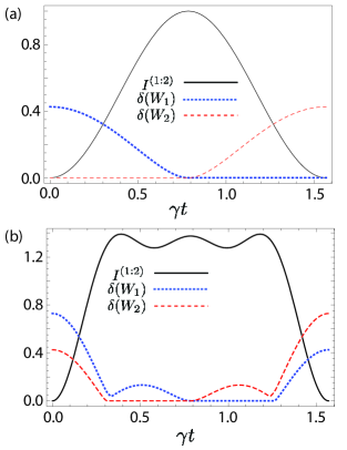
Figure 1: (Color online): Mutual information (black solid line) and negativity of the local Wigner functions $W_{1}(q_{1},p_{1})$ (blue dotted line) and $W_{2}(q_{2},p_{2})$ (red dashed line ) as function of the dimensionless time $\gamma t$ for two different cases, (a) $(k,\ell)=(1,0)$ and (b) $(k,\ell)=(2,1)$, in order to illustrate how the mutual information depends on the non-classicality of local states of the system. It is possible to note the inversion of the negativities in both cases, as well as that the minimum value of them is reached when the mutual information is maximum. We considered unities such that $\hbar=m=\omega=1$.

IV Dissipative dynamics

For this purpose, we shall assume that the states of the subsystems $(q_{1},p_{1})$ and $(q_{2},p_{2})$ are Gaussian, i.e. $W_{1}(q_{1},p_{1})$ and $W_{2}(q_{2},p_{2})$ are completely characterized by their first moments and covariance matrix, and defining our system as being $W_{sys}\equiv W_{1}(q_{1},p_{1})$. Besides, we consider that $\Gamma$ and $\gamma$ are constants mediating the coupling between the thermal reservoir with the subsystem $(q_{1},p_{1})$, and the subsystems $(q_{1},p_{1})$ and $(q_{2},p_{2})$, respectively. Figure (2) shows an illustration of the considered dissipative process. We restrict our attention to investigate the dynamics of $W_{sys}$ and observe how the coupling $\gamma$ impacts its dissipative dynamics when in thermal contact with a Markovian environment. From a physical point of view, we consider that the time evolution of $W_{sys}$ is strictly Markovian when $\gamma\rightarrow 0$. Moreover, in tracing out the degrees of freedom $(q_{2},p_{2})$ and restricting our attention only to $W_{sys}$, we are assuming that the coupling between the thermal environment and the degrees of freedom $(q_{2},p_{2})$ is sufficiently weak such that it does not cause any effect on the evolution of $W_{sys}$.

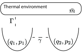
Figure 2: Illustration of the system which is considered, $W_{sys}=W_{1}(q_{1},p_{1})$, coupled to another quantum oscillator $(q_{2},p_{2})$ by the coupling $\gamma$, and also coupled to a thermal environment with coupling $\Gamma$. We are considering that the coupling between the thermal environment and the quantum oscillator $(q_{2},p_{2})$ is sufficiently weak such that any effect due to it is negligible for the evolution of the system $W_{sys}$.

Figure (3) shows the fidelity (black solid line) and the normalized coherence (red dashed line) for a heating process, i.e. $\bar{n}>\bar{m}$, with $\bar{n}$ and $\bar{m}$ the mean number of photons of the system and the thermal environment, respectively. In order to guarantee that the environment itself generates a Markovian evolution on the system, we show the case in which $\gamma=0$, Fig. (3)(inset), i.e. there is no coupling of the system with any other degree of freedom. In the case with $\gamma=0.1$, we observe the non-monotonic behavior of the fidelity and the increase of the coherence in some time intervals.

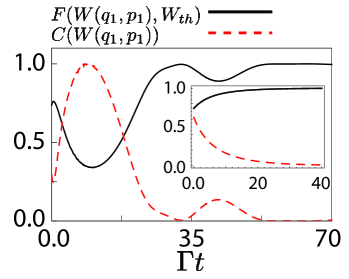
Figure 3: (Color online): Fidelity and normalized coherence for the system defined as $W_{sys}=W_{1}(q_{1},p_{1})$ as function of the dimensionless time of thermalization with the thermal environment for $\gamma=0.1$. The inset shows the same quantities for $\gamma=0$. We considered $(x,p_{x},y,p_{y})=(1,1,1,1)$, $(\bar{n},\bar{m})=(2,4)$ with $\bar{n}$ and $\bar{m}$ the mean number of photons of the system and thermal environment, respectively, and $\hbar=m=\omega=1$.

Non-Markonian-like effect

In Fig. (3) we note that the fidelity for $\gamma\neq 0$ presents a non-monotonic behavior during the thermalization process with a thermal environment. This profile in the fidelity has been recently associated to a non-Markovian dynamics on the system characterizing an information backflow from the environment to the system Breuer2016 ; Rendell2010 ; Rivas2010 ; Breuer2009 . Here the considered thermal environment generates a Markovian dynamics on the system, as we note from the Fig. (3) (inset) for $\gamma=0$. Thus, any non-Markovian-like behavior arises due to the coupling constant $\gamma\neq 0$. Physically, the fidelity is a witness of non-Markovianity and the condition is that $F(\rho_{1}(\tau),\rho_{2}(\tau))\leq F(\rho_{1}(t),\rho_{2}(t))$, with $\rho_{1(2)}$ two arbitrary states of the system and $\tau$ and $t$ arbitrary times such that $\tau>t$ Breuer2016 ; Rendell2010 . Figure (3) presents basically two time intervals for $\gamma=0.1$ with this behavior. Furthermore, the coherence increases during the same time intervals, evidencing a memory effect on the system. Again, it is worth to note that this behavior is exclusively due to the coupling $\gamma$ and does not depend on the structure of the thermal environment. Here, a similar experiment as performed in Ref. Cuevas2019 could be useful to simulate the non-Markovian-like effect employing coherent (Gaussian) states in a quantum optical device.

V Trapped ions approach for two-coupled harmonic oscillators

In this section we present some well-know results that show the ability to implement our findings in trapped ions, employing the vibrational modes of the ion. The simplest ion trap Hamiltonian reads Ortiz2017 ,

$$H=H_{0}+H_{I},$$ (31)

where $H_{I}$ is the interaction Hamiltonian and $H_{0}$ represents the free dynamics of the ion and is given by

$$H_{0}=\frac{1}{2}\hbar\omega_{0}\sigma_{z}+\hbar\omega_{x}a_{x}a_{x}^{\dagger}+\hbar\omega_{y}a_{y}a_{y}^{\dagger},$$ (32)

with $\omega_{0}$ the transition frequency associated to the electronic modes, $\sigma_{z}$ the Pauli matrix, $\omega_{i}$, $i=x,y$ the natural frequencies relative to the vibrational models, which are written in terms of the creation and annihilation operators $a_{i}$ and $a_{i}^{\dagger}$. In general, the complexity of the dynamics depends on the well-known Lamb-Dicke parameters, $\eta_{i}=k_{0}/\sqrt{2\omega_{i}m}$, with $k_{0}$ and $m$ the wavevector component and mass of the ion, respectively. Let consider the Lamb-Dicke regime, $\eta_{x},\eta_{y}\ll 1$. In Ref. Ortiz2017 , the interaction Hamiltonian is expanding in terms of the Lamb-Dicke parameters,

$$H_{I}=H^{(0)}+\eta_{x}H_{x}^{(1)}+\eta_{y}H_{y}^{(1)}-\eta_{x}^{2}H_{x}^{(2)}-\eta_{y}^{2}H_{y}^{(2)}-2\eta_{x}\eta_{y}^{2}H_{xy}^{(2)}+\mathcal{O}(\eta_{i}^{3}).$$ (33)

Focusing only on the first-order terms (the other terms can be seen in Ref. Ortiz2017 ), they are given by

$$H_{i}^{(1)} =\frac{1}{2}\hbar\Omega\left(e^{-i(\Delta+\omega_{i})t}\sigma_{+}\hat{i}+e^{i(\Delta+\omega_{i})t}\sigma_{-}\hat{i}^{\dagger}\right)$$

$$+\frac{1}{2}\hbar\Omega\left(e^{-i(\Delta-\omega_{i})t}\sigma_{+}\hat{i}^{\dagger}+e^{i(\Delta-\omega_{i})t}\sigma_{-}\hat{i}\right),$$ (34)

with $\Omega$ the Rabbi frequency, $\Delta=\omega_{L}-\omega_{0}$ the radiation-atom detuning, $\omega_{L}$ the frequency of the applied electric field, and $\sigma_{-}=|e\rangle\langle g|$ and $\sigma_{+}=|g\rangle\langle e|$ are the operators associated to the electronic transitions. This type of interaction can be useful to experimentally simulate the first part of our results, ie., the use of the mutual information in the exchange of negativity between two Fock states. The interaction Hamiltonian in Eq. (34) allows to create the respective Fock states, once the electronic mode can be used to create or annihilate phonons in the vibrational modes.

On the other hand, to consider the dissipative dynamics, as in our second result, we can use Ref. Zhong2018 and explore the generation of cat states in trapped ions setup. Following Ref.Zhong2018 we can write the master equation for a ion composed of one electronic mode and two vibrational modes as,

$$\frac{d\rho}{dt} =-i[H_{i},\rho]+\frac{\Gamma}{2}\left(2\sigma_{-}\rho\sigma_{+}-\sigma_{+}\sigma_{-}\rho-\rho\sigma_{-}\sigma_{+}\right)$$ (35)

$$+\frac{\gamma_{x}}{2}(2a_{x}\rho a_{x}^{\dagger}-a_{x}^{\dagger}a_{x}\rho-\rho a_{x}a_{x}^{\dagger})+\frac{\gamma_{y}}{2}(2a_{y}\rho a_{y}^{\dagger}-a_{y}^{\dagger}a_{y}\rho-\rho a_{y}a_{y}^{\dagger}),$$ (36)

with $\hbar=1$, and $\Gamma$, $\gamma_{i}$ are the decay rates to the electronic and vibrational modes, respectively, and the state $\rho$ encodes both electronic and vibrational modes. Of course, the coupling with the reservoir can be turned off for one vibrational mode, thus the simulation of our results in section IV could be experimentally implemented.

VI Conclusions

In this work we have considered a system composed of two-coupled harmonic oscillators and explored some properties related to the unitary and the dissipative dynamics. In the first case, we investigated how the mutual information between two states allows to transfer the non-Gaussian aspect (quantified by the negativity of the Wigner function) between two Fock states. On the other hand, for dissipative dynamics of Gaussian states, it was possible to note that for Gaussian states initially with coherence, the effect of the coupling between the two subsystems may generate some non-trivial behavior in the fidelity comparing the state of the system and the asymptotic one, similarly to a non-Markovian-like effect. Moreover, the same effect can be observed in the coherence during the time evolution, with coherence revivals in specific time intervals.

Among some experimental platforms which could be useful to experimentally simulate our results, for instance, quantum optics and optomechanical systems, we highlighted the trapped ions setup, where the vibrational modes of the ion could encode the two-coupled harmonic oscillators we investigated here, and the electronic mode could be useful to prepare the desired states. Finally, we reinforce that the quantum information quantities used here have been largely employed in quantum thermodynamics protocols, showing that our results can be also applied to this field.

Appendix A Derivation of the Wigner function for two-coupled harmonic oscillators in phase-space

In this appendix we derived with some details the Wigner function for two-coupled harmonic oscillators, described in the Hamiltonian (23). By introducing the creation and annihilation operators,

$$a_{i}=\frac{\alpha}{\sqrt{2\hbar\alpha\beta}}q_{i}+i\frac{\beta}{\sqrt{2\hbar\alpha\beta}}p_{i},$$ (37)

$$a_{i}^{\dagger}=\frac{\alpha}{\sqrt{2\hbar\alpha\beta}}q_{i}-i\frac{\beta}{\sqrt{2\hbar\alpha\beta}}p_{i},$$ (38)

with $i=1,2$, these operators $a_{i}$ and $a_{i}^{\dagger}$ satisfy the following condition,

$$\left[\hat{a}_{i},\hat{a}_{j}^{\dagger}\right]=\delta_{ij},\quad\left[\hat{a}_{i},\hat{a}_{i}^{\dagger}\right]=\left[\hat{a}_{j},\hat{a}_{j}^{\dagger}\right]=0.$$ (39)

Now we can write the equation (23) as,

$$H(q_{i},p_{i}) =2\hbar\alpha\beta\left(a_{1}^{\dagger}a_{1}+a_{2}^{\dagger}a_{2}\right)$$

$$-i\hbar\gamma(a_{1}a_{2}^{\dagger}-a_{2}a_{1}^{\dagger})$$ (40)

Note that still there exists a coupling between operators $a_{1}$ and $a_{2}$. Then, it is interesting to define the new set of creation and annihilation operators,

$$A_{\pm}=\frac{1}{\sqrt{2}}\left(a_{1}\mp ia_{2}\right),\quad A_{\pm}^{\dagger}=\frac{1}{\sqrt{2}}\left(a_{1}^{\dagger}\pm ia_{2}^{\dagger}\right),$$ (41)

with these operators obeying the following commutation relations,

$$\left[A_{\pm},A_{\pm}\right] =\left[A_{\pm},A_{\mp}\right]=0$$

$$\left[A_{\pm}^{\dagger},A_{\pm}^{\dagger}\right] =\left[A_{\pm}^{\dagger},\hat{A}\right]=0,$$

$$\left[A_{\pm},A_{\pm}^{\dagger}\right] =\left[A_{\mp},A_{\mp}^{\dagger}\right]=1$$

$$\left[A_{\mp},A_{\pm}^{\dagger}\right] =\left[A_{\pm},A_{\mp}^{\dagger}\right]=0$$

Therefore, the Hamiltonian (40) is given by,

$$H(q_{i},p_{i}) =2\hbar\alpha\beta\left(A_{+}^{\dagger}A_{+}+A_{-}^{\dagger}A_{-}+1\right)$$

$$-\hbar\gamma\left(A_{+}^{\dagger}A_{+}-A_{-}^{\dagger}A_{-}\right).$$ (42)

The next step is to rewrite the Moyal product (6) in terms of these new operators. Denoting by $A_{\pm}^{+}$ and $A_{\pm}$ as the Weyl transform of the operators $A_{\pm}^{\dagger}$ and $A_{\pm}$, respectively, we can write the Moyal product as,

$$\star =\exp\left[\frac{1}{2}\left(\overleftarrow{\partial}_{A_{+}}\overrightarrow{\partial}_{A_{+}^{+}}-\overleftarrow{\partial}_{A_{+}^{+}}\overrightarrow{\partial}_{A_{+}}\right)\right]$$

$$\times\text{exp}\left[\frac{1}{2}\left(\overleftarrow{\partial}_{A_{-}}\overrightarrow{\partial}_{A_{-}^{+}}-\overleftarrow{\partial}_{A_{-}^{+}}\overrightarrow{\partial}_{A_{-}}\right)\right],$$

with $A_{+}^{+}\star A_{+}=A_{+}^{+}A_{+}-1/2.$

Defining new variables $\eta_{1}=A_{+}^{+}A_{+}$ and $\eta_{2}=A_{-}^{+}A_{-}$, the Weyl transform of the Hamiltonian (42) reads,

$$H^{W}(\eta_{1},\eta_{2})=(2\hbar\alpha\beta-\hbar\gamma)\eta_{1}+(2\hbar\alpha\beta+\hbar\gamma)\eta_{2}.$$ (43)

In addition, applying the so-called stargenvalue equation (9) for the system,

$$H^{W}(\eta_{1},\eta_{2})\star W(\eta_{1},\eta_{2})=EW(\eta_{1},\eta_{2}),$$ (44)

we have that,

$$H^{W}(\eta_{1},\eta_{2})\star W(\eta_{1},\eta_{2}) =[(2\hbar\alpha\beta-\hbar\gamma)\eta_{1}+(2\hbar\alpha\beta+\hbar\gamma)\eta_{2}$$

$$+\frac{1}{2}(2\hbar\alpha\beta-\hbar\gamma)+\left(A_{+}^{+}\frac{\partial}{\partial A_{+}^{+}}-A_{+}\frac{\partial}{\partial A_{+}}\right)$$

$$+\frac{1}{2}(2\hbar\alpha\beta+\hbar\gamma)+\left(A_{-}^{+}\frac{\partial}{\partial A_{-}^{+}}-A_{-}\frac{\partial}{\partial A_{-}}\right)$$

$$-\frac{1}{4}(2\hbar\alpha\beta-\hbar\gamma)-\frac{\partial^{2}}{\partial A_{+}\partial A_{+}^{+}}$$

$$-\frac{1}{4}(2\hbar\alpha\beta+\hbar\gamma)-\frac{\partial^{2}}{\partial A_{-}\partial A_{-}^{+}}]$$

$$=EW(\eta_{1},\eta_{2}).$$

After some mathematical manipulations we obtain two uncoupled differential equations given by,

$$\left[\eta_{1(2)}-\frac{1}{4}\left(\frac{\partial}{\partial\eta_{1(2)}}+\eta_{1(2)}\frac{\partial^{2}}{\partial\eta_{1(2)}^{2}}\right)-E_{1(2)}\right]$$

$$\times\chi_{1(2)}(\eta_{1(2)}) =0$$ (45)

The explicit solutions of Eqs. (45) can be written in terms of the Laguerre polynomials,

$$\chi_{1(2)}(\eta_{1(2)})=(-1)^{n_{1(2)}}\exp\left[-2\chi_{1(2)}\right]L_{n_{1(2)}}\left[4\chi_{1(2)}\right],$$ (46)

with $n_{1(2)}$ non-negative integers and $n_{1(2)}=(E_{1(2)}-1/2)$, resulting in,

$$E_{n_{1},n_{2}}=2\hbar\alpha\beta\left(n_{1}+n_{2}+1\right)+\hbar\gamma\left(n_{1}-n_{2}\right).$$ (47)

Finally, writing as function of canonical phase-space variables, the Wigner function in (24) is obtained.

References

- (1) A. Bermudez, T. Schaetz, and M. B. Plenio, Dissipation-Assisted Quantum Information Processing with Trapped Ions, Phys. Rev. Lett. , 110502 (2013).
- (2) K. Marshall and C. Weedbrook, Device-independent quantum cryptography for continuous variables, Phys. Rev. A 90, 042311 (2014).
- (3) P. Papanastasiou, C. Ottaviani, and S. Pirandola, Finite-size analysis of measurement-device-independent quantum cryptography with continuous variables, Phys. Rev. A 96, 042332 (2017).
- (4) C. Ottaviani, S. Mancini, and S. Pirandola, Two-way Gaussian quantum cryptography against coherent attacks in direct reconciliation, Phys. Rev. A 92, 062323 (2015).
- (5) M. Perarnau-Llobet, A. González-Tudela, J. I. Cirac, Multimode Fock states with large photon number: effective descriptions and applications in quantum metrology, arXiv:1910.03323.
- (6) Pietro Liuzzo-Scorpo, Andrea Mari, Vittorio Giovannetti, and Gerardo Adesso, Optimal Continuous Variable Quantum Teleportation with Limited Resources, Phys. Rev. Lett. 119, 120503 (2017).
- (7) P. A. Camati, J. F. G. Santos, and R. M. Serra, Coherence effects in the performance of the quantum Otto heat engine, Phys. Rev. A 99, 062103 (2019).
- (8) R. Dann and R. Kosloff, Quantum Signatures in the Quantum Carnot Cycle, arXiv:1906.0694.
- (9) S.Su, W. Shen, J. Du, and J. Chen, Coherence induced work in quantum heat engines with Larmor precession, arXiv:1908.06443.
- (10) W. H. Zurek, Reversibility and Stability of Information Processing Systems, Phys. Rev. Lett. , 391 (1984).
- (11) F. Arute, K. Arya, R. Babbush, et al. Quantum supremacy using a programmable superconducting processor. Nature 574, 505-510 (2019).
- (12) Z. Gedik, I. A. Silva, B. Çakmak, G. Karpat, E. L. G. Vidoto, D. O. Soares-Pinto, E. R. deAzevedo and F. F. Fanchini, Computational speed-up with a single qudit, Sci. Rep. 5, 14671 (2015).
- (13) M. H. Partovi, Entanglement versus stosszahlansatz: disappearance of the thermodynamic arrow in a high-correlation environment. Phys. Rev. E 77, 021110 (2008).
- (14) S. Jevtic, D. Jennings, and T. Rudolph, Maximally and minimally correlated states attainable within a closed evolving system. Phys. Rev. Lett. 108, 110403 (2012).
- (15) K. Micadei, J.P.S. Peterson, A.M. Souza et al. Reversing the direction of heat flow using quantum correlations. Nat Commun 10, 2456 (2019).
- (16) S. Hamedani Raja, M. Borrelli, R. Schmidt, J. P. Pekola, S. Maniscalco, Thermodynamic fingerprints of non-Markovianity, Phys. Rev. A 97, 032133 (2018).
- (17) M. Cianciaruso, S. Maniscalco, and G. Adesso, Role of non-Markovianity and backflow of information in the speed of quantum evolution, Phys. Rev. A 96, 012105 (2017).
- (18) P. A. Camati, J. F. G. Santos, and R. M. Serra, Employing Non-Markovian effects to improve the performance of a quantum Otto refrigerator. In preparation.
- (19) W. Ge, B. C. Sawyer, J. W. Britton, K. Jacobs, J. J. Bollinger, and M. Foss-Feig, Trapped Ion Quantum Information Processing with Squeezed Phonons, Phys. Rev. Lett. 122, 030501 (2019).
- (20) A. Carlini, A. Mari, and V. Giovannetti, Time-optimal thermalization of single-mode Gaussian states, Phys. Rev. A , 052324 (2014).
- (21) F. Albarelli, U. S.-Bennett, and A. Serafini, Locally optimal control of continuous-variable entanglement, Phys. Rev. A 98, 062312 (2018).
- (22) D.Su, C. R. Myers, and K. K. Sabapathy, Conversion of Gaussian states to non-Gaussian states using photon-number-resolving detectors, Phys. Rev. A 100, 052301 (2019).
- (23) G. Adesso, S. Ragy, and A. R. Lee, Continuous variable quantum information: Gaussian states and beyond, Open Syst. Inf. Dyn., 1440001 (2014).
- (24) C. Weedbrook, S. Pirandola, R. García-Patrón, N. J. Cerf, T. C. Ralph, J. H. Shapiro, and S. Lloyd, Gaussian quantum information, Rev. Mod. Phys. 84, 621 (2012).
- (25) H. P. Breuer and F. Petruccione, The Theory of Open Quantum Systems, (Oxdord University Press, Oxford, 2002).
- (26) M. A. Nielsen and I. L. Chuang, Quantum Computation and Quantum Information, (Cambridge University Press, Cambridge, 2010).
- (27) M. O. Scully and M. S. Zubairy, Quantum optics, (Cambridge University Press, Cambridge, 2012).
- (28) D. Leibfried, R. Blatt, C. Monroe, and D. Wineland, Quantum dynamics of single trapped ions, Rev. Mod. Phys. 75, 281 (2003).
- (29) C. D. Bruzewicz, J. Chiaverini, R.t McConnell, and J.M. Sage, Trapped-Ion Quantum Computing: Progress and Challenges, arXiv:1904.04178.
- (30) G. W. Biedermann, X. Wu, L. Deslauriers, S. Roy, C. Mahadeswaraswamy, and M. A. Kasevich, Testing gravity with cold-atom interferometers, Phys. Rev. A 91, 033629 (2015).
- (31) Y. Han, C. Zhu, X. Huang, Y. Yang, Electromagnetic control of nonclassicality in cavity QED system, Physical Review A 98, 033828 (2018).
- (32) A. V. Dodonov, D. Valente, T. Werlang, Quantum power boost in a nonstationary cavity-QED quantum heat engine, J. Phys. A: Math. Theor. 51, 365302 (2018).
- (33) C. K Zachos, D. B Fairlie, and T. L Curtright, Quantum Mechanics in Phase Space: An Overview with Selected Papers, (World Scientific Pub. Co. Inc., Singapure, 2005).
- (34) E. Wigner, On the Quantum Correction For Thermodynamic Equilibrium, Phys. Rev. 40, 749 (1932).
- (35) W. B. Case, Wigner functions and Weyl transforms for pedestrians, Am. J. Phys. 76, 937 (2008).
- (36) K.S. Chou, J.Z. Blumoff, C.S. Wang et al. Deterministic teleportation of a quantum gate between two logical qubits. Nature 561, 368 (2018).
- (37) J. F. G. Santos, A. E. Bernardini, and C. Bastos, Probing phase-space noncommutativity through quantum mechanics and thermodynamics of free particles and quantum rotors, Physica A , 340 (2015)
- (38) J. F. G. Santos and A. E. Bernardini, Gaussian fidelity distorted by external fields, Physica A , 75 (2016).
- (39) A. E. Bernardini and O. Bertolami, Probing phase-space noncommutativity through quantum beating, missing information and the thermodynamic limit, Phys. Rev. A , 012101 (2013).
- (40) M. Rosenbaum and J. D. Vergara, The -value equation and Wigner distributions in noncommutative Heisenberg algebras, Gen. Rel. Grav. 38, 607 (2006).
- (41) J. Steinbach, J. Twamley, and P. L. Knight, Engineering two-mode interactions in ion traps, Phys. Rev. A 56, 4815 (1997).
- (42) C. Monroe, D. M. Meekhof, B. E. King, and D. J. Wineland, A “Schrödinger Cat” Superposition State of an Atom, Science 272, 5265 (1996).
- (43) Z.-R. Zhong, X.-J. Huang, Z.-B.Yang, L.-T. Shen, and S.-B. Zheng, Generation and stabilization of entangled coherent states for the vibrational modes of a trapped ion, Phys. Rev. A 98, 032311 (2018).
- (44) L. Ortiz-Gutiérrez, B. Gabrielly, L. F. Muñoz, K. T. Pereira, J. G. Filgueiras, and A. S. Villar, Continuous variables quantum computation over the vibrational modes of a single trapped ion, Optics Communications 397, (2017).
- (45) F. Albarelli, M. G. Genoni, and M. G. A. Paris, Resource theory of quantum non-Gaussianity and Wigner negativity, Phys. Rev. A 98, 052350 (2018).
- (46) K.-P. Marzlin and S. Deering, The Moyal equation for open quantum systems, J. Phys. A: Math. Theor. 48, 205301 (2015).
- (47) G. Manfredi, and M. R. Feix, Entropy and Wigner functions, Phys. Rev. E 62, 4665 (2000).
- (48) A. Kenfack and K. Zyczkowski, Negativity of the Wigner function as an indicator of non-classicality, J. Opt. B: Quantum Semiclass. Opt. 6 396 (2004).
- (49) R. P. Rundle, P. W. Mills, Todd Tilma, J. H. Samson, and M. J. Everitt, Simple procedure for phase-space measurement and entanglement validation, Phys. Rev. A Phys. Rev. A 96, 022117 (2017).
- (50) M.Walschaers, C. Fabre, V. Parigi, and N. Treps, Entanglement and Wigner Function Negativity of Multimode Non-Gaussian States, Phys. Rev. Lett. 119, 183601 (2017).
- (51) I. I. Arkhipov, A.Barasiński, and J. Svozilík, Negativity volume of the generalized Wigner function as an entanglement witness for hybrid bipartite states, Sci. Rep. 8, 16955 (2018).
- (52) G. Nogues, A. Rauschenbeutel, S. Osnaghi, P. Bertet, M. Brune, J. M. Raimond, S. Haroche, L. G. Lutterbach, and L. Davidovich, Measurement of a negative value for the Wigner function of radiation, Phys. Rev. A 62, 054101 (2000).
- (53) R.Raussendorf, D. E. Browne, N. Delfosse, C. Okay, and J. Bermejo-Vega, Contextuality and Wigner-function negativity in qubit quantum computation, Phys. Rev. A 95, 052334 (2014).
- (54) X.-B. Wang, T. Hiroshima, A. Tomita, and M. Hayashi, Quantum information with Gaussian states, Physics Reports 448, (2007).
- (55) A. Serafini, Quantum Continuous Variables. A primer of Theoretical Methods, (CRC Press, Boca Raton, 2017).
- (56) A. S. Holevo, Some statistical problems for quantum Gaussian states, IEEE Trans. Inf. Theory , 533 (1975).
- (57) H. Scutaru, Fidelity for displaced squeezed states and the oscillator semigroup, J. Phys. A , 3659 (1998).
- (58) J. DiGuglielmo, B. Hage, A. Franzen, J. Fiurášek, and Roman Schnabel, Experimental characterization of Gaussian quantum-communication channels, Phys. Rev. A 76, 012323 (2007).
- (59) A. Winter and D. Yang, Operational Resource Theory of Coherence, Phys. Rev. Lett. 116, 120404 (2016).
- (60) T. Baumgratz, M. Cramer, and M. B. Plenio, Quantifying coherence, Phys. Rev. Lett. 113, 140401 (2014).
- (61) T. Feldmann and R. Kosloff, Quantum lubrication: Suppression of friction in a first-principles four-stroke heat engine, Phys. Rev. E 73, 025107(R) (2006).
- (62) Y. Rezek and R. Kosloff, Irreversible performance of a quantum harmonic heat engine, New J. Phys. 8, 83 (2006).
- (63) J. Xu, Quantifying coherence of Gaussian states, Phys. Rev. A , 032111 (2016).
- (64) A. Carlini, A. Mari, and V. Giovanneti, Time-Optimal Thermalization of Single-Mode Gaussian States, Phys. Rev. A , 052324 (2014).
- (65) A. M. Jayannavar and Mamata Sahoo, Charged particle in a magnetic field: Jarzynski equality, Phys. Rev. A 75, 032102 (2007).
- (66) E. Muñoz and F. J. Peña, Magnetically driven quantum heat engine Phys. Rev. E 89, 052107 (2014).
- (67) J. F. G. Santos, A. E. Bernardini, Quantum engines and the range of the second law of thermodynamics in the noncommutative phase-space, Eur. Phys. J. Plus 132, 260 (2017).
- (68) Á. Rivas, S. F. Huelga, and M. B. Plenio, Entanglement and Non-Markovianity of Quantum Evolutions, Phys. Rev. Lett. , 050403 (2010).
- (69) H.-P. Breuer, E.-M. Laine, and J. Piilo, Measure for the Degree of Non-Markovian Behavior of Quantum Processes in Open Systems, Phys. Rev. Lett. , 210401 (2009).
- (70) H.-P. Breuer, E.-M. Laine, J. Piilo, and B. Vacchini, Colloquium: Non-Markovian dynamics in open quantum systems, Rev. Mod. Phys. , 021002 (2016).
- (71) A. K. Rajagopal, A. R. Usha Devi, and R. W. Rendell, Kraus representation of quantum evolution and fidelity as manifestations of Markovian and non-Markovian forms A., Phys. Rev. A , 042107 (2010).
- (72) Á. Cuevas, A. Geraldi, C. Liorni et al. All-optical implementation of collision-based evolutions of open quantum systems. Sci Rep 9, 3205 (2019).