Privacy-Preserving Multiple Tensor Factorization for Synthesizing Large-Scale Location Traces with Cluster-Specific Features

Abstract

With the widespread use of LBSs (Location-based Services), synthesizing location traces plays an increasingly important role in analyzing spatial big data while protecting user privacy. In particular, a synthetic trace that preserves a feature specific to a cluster of users (e.g., those who commute by train, those who go shopping) is important for various geo-data analysis tasks and for providing a synthetic location dataset. Although location synthesizers have been widely studied, existing synthesizers do not provide sufficient utility, privacy, or scalability, hence are not practical for large-scale location traces. To overcome this issue, we propose a novel location synthesizer called PPMTF (Privacy-Preserving Multiple Tensor Factorization). We model various statistical features of the original traces by a transition-count tensor and a visit-count tensor. We factorize these two tensors simultaneously via multiple tensor factorization, and train factor matrices via posterior sampling. Then we synthesize traces from reconstructed tensors, and perform a plausible deniability test for a synthetic trace. We comprehensively evaluate PPMTF using two datasets. Our experimental results show that PPMTF preserves various statistical features including cluster-specific features, protects user privacy, and synthesizes large-scale location traces in practical time. PPMTF also significantly outperforms the state-of-the-art methods in terms of utility and scalability at the same level of privacy.

1 Introduction

LBSs (Location-based Services) have been used in a variety of applications such as POI (Point-of-Interest) search, route finding, and geo-social networking. Consequently, numerous location traces (time-series location trails) have been collected into the LBS provider. The LBS provider can provide these location traces (also called spatial big data [61]) to a third party (or data analyst) to perform various geo-data analysis tasks; e.g., finding popular POIs [76], semantic annotation of POIs [19, 71], modeling human mobility patterns [17, 40, 42, 64], and road map inference [5, 41].

Although such geo-data analysis is important for industry and society, some important privacy issues arise. For example, users’ sensitive locations (e.g., homes, hospitals), profiles (e.g., age, profession) [33, 44, 74], activities (e.g., sleeping, shopping) [39, 74], and social relationships [6, 24] can be estimated from traces.

Synthesizing location traces [8, 15, 32, 36, 65, 73] is one of the most promising approaches to perform geo-data analysis while protecting user privacy. This approach first trains a generative model from the original traces (referred to as training traces). Then it generates synthetic traces (or fake traces) using the trained generative model. The synthetic traces preserve some statistical features (e.g., population distribution, transition matrix) of the original traces because these features are modeled by the generative model. Consequently, based on the synthetic traces, a data analyst can perform the various geo-data analysis tasks explained above.

In particular, a synthetic trace that preserves a feature specific to a cluster of users who exhibit similar behaviors (e.g., those who commute by car, those who often go to malls) is important for tasks such as semantic annotation of POIs [19, 71], modeling human mobility patterns [17, 40, 42, 64], and road map inference [5, 41]. The cluster-specific features are also necessary for providing a synthetic dataset for research [30, 52] or anonymization competitions [2]. In addition to preserving various statistical features, the synthetic traces are (ideally) designed to protect privacy of users who provide the original traces from a possibly malicious data analyst or any others who obtain the synthetic traces.

Ideally, a location synthesizer should satisfy the following three features: (i) high utility: it synthesizes traces that preserve various statistical features of the original traces; (ii) high privacy: it protect privacy of users who provide the original traces; (iii) high scalability: it generates numerous traces within an acceptable time; e.g., within days or weeks at most. All of these features are necessary for spatial big data analysis or providing a large-scale synthetic dataset.

Although many location synthesizers [8, 12, 13, 15, 28, 32, 36, 65, 73] have been studied, none of them are satisfactory in terms of all three features:

Related work.  Location privacy has been widely studied ([11, 27, 37, 57] presents related surveys) and synthesizing location traces is promising in terms of geo-data analysis and providing a dataset, as explained above. Although location synthesizers have been widely studied for over a decade, Bindschaedler and Shokri [8] showed that most of them (e.g., [15, 32, 36, 65, 73]) do not satisfactorily preserve statistical features (especially, semantic features of human mobility, e.g., “many people spend night at home”), and do not provide high utility.

A synthetic location traces generator in [8] (denoted by SGLT) is a state-of-the-art location synthesizer. SGLT first trains semantic clusters by grouping semantically similar locations (e.g., homes, offices, and malls) based on training traces. Then it generates a synthetic trace from a training trace by replacing each location with all locations in the same cluster and then sampling a trace via the Viterbi algorithm. Bindschaedler and Shokri [8] showed that SGLT preserves semantic features explained above and therefore provides high utility.

However, SGLT presents issues of scalability, which is crucially important for spatial big data analysis. Specifically, the running time of semantic clustering in SGLT is quadratic in the number of training users and cubic in the number of locations. Consequently, SGLT cannot be used for generating large-scale traces. For example, we show that when the numbers of users and locations are about $200000$ and $1000$, respectively, SGLT would require over four years to execute even by using $1000$ nodes of a supercomputer in parallel.

Bindschaedler et al. [9] proposed a synthetic data generator (denoted by SGD) for any kind of data using a dependency graph. However, SGD was not applied to location traces, and its effectiveness for traces was unclear. We apply SGD to location traces, and show that it cannot preserve cluster-specific features (hence cannot provide high utility) while keeping high privacy. Similarly, the location synthesizers in [12, 13, 28] generate traces only based on parameters common to all users, and hence do not preserve cluster-specific features.

Our contributions.  In this paper, we propose a novel location synthesizer called PPMTF (Privacy-Preserving Multiple Tensor Factorization), which has high utility, privacy, and scalability. Our contributions are as follows:

• We propose PPMTF for synthesizing traces. PPMTF models statistical features of training traces, including cluster-specific features, by two tensors: a transition-count tensor and visit-count tensor. The transition-count tensor includes a transition matrix for each user, and the visit-count tensor includes a time-dependent histogram of visited locations for each user. PPMTF simultaneously factorizes the two tensors via MTF (Multiple Tensor Factorization) [35, 66], and trains factor matrices (parameters in our generative model) via posterior sampling [68]. Then it synthesizes traces from reconstructed tensors, and performs the PD (Plausible Deniability) test [9] to protect user privacy. Technically, this work is the first to propose MTF in a privacy preserving way, to our knowledge.

• We comprehensively show that the proposed method (denoted by PPMTF) provides high utility, privacy, and scalability (for details, see below).

Regarding utility, we show that PPMTF preserves all of the following statistical features.

(a) Time-dependent population distribution.  The population distribution (i.e., distribution of visited locations) is a key feature to find popular POIs [76]. It can also be used to provide information about the number of visitors at a specific POI [29]. The population distribution is inherently time-dependent. For example, restaurants have two peak times corresponding to lunch and dinner periods [71].

(b) Transition matrix.  The transition matrix is a main feature for modeling human movement patterns [42, 64]. It is used for predicting the next POI [64] or recommending POIs [42].

(c) Distribution of visit-fractions.  A distribution of visit-fractions (or visit-counts) is a key feature for semantic annotation of POIs [19, 71]. For example, [19] reports that many people spend $60\%$ of the time at their home and $20\%$ of the time at work/school. [71] reports that most users visit a hotel only once, whereas $5\%$ of users visit a restaurant more than ten times.

(d) Cluster-specific population distribution.  At an individual level, a location distribution differs from user to user, and forms some clusters; e.g., those who live in Manhattan, those who commute by car, and those who often visit malls. The population distribution for such a cluster is useful for modeling human location patterns [17, 40], road map inference [5, 41], and smart cities [17].

We show that SGD does not consider cluster-specific features in a practical setting (similarly, [12, 13, 28] do not preserve cluster-specific features), and therefore provides neither (c) nor (d). In contrast, we show that PPMTF provides all of (a)-(d). Moreover, PPMTF automatically finds user clusters in (d); i.e., manual clustering is not necessary. Note that user clustering is very challenging because it must be done in a privacy preserving manner (otherwise, user clusters may reveal information about users who provide the original traces).

Regarding privacy, there are two possible scenarios about parameters of the generative model: (i) the parameters are made public and (ii) the parameters are kept secret (or discarded after synthesizing traces) and only synthetic traces are made public. We assume scenario (ii) in the same way as [8]. In this scenario, PPMTF provides PD (Plausible Deniability) in [9] for a synthetic trace. Here we use PD because both SGLT [8] and SGD [9] use PD as a privacy metric (and others [12, 13, 28] do not preserve cluster-specific features). In other words, we can evaluate how much PPMTF advances the state-of-the-art in terms of utility and scalability at the same level of privacy. We also empirically show that PPMTF can prevent re-identification (or de-anonymization) attacks [63, 26, 47] and membership inference attacks [62, 31] in scenario (ii). One limitation is that PPMTF does not guarantee privacy in scenario (i). We clarify this issue at the end of Section 1.

Regarding scalability, for a larger number $|\mathcal{U}|$ of training users and a larger number $|\mathcal{X}|$ of locations, PPMTF’s time complexity $O(|\mathcal{U}||\mathcal{X}|^{2})$ is much smaller than SGLT’s complexity $O(|\mathcal{U}|^{2}|\mathcal{X}|^{3})$. Bindschaedler and Shokri [8] evaluated SGLT using training traces of only $30$ users. In this paper, we use the Foursquare dataset in [69] (we use six cities; $448839$ training users in total) and show that PPMTF generates the corresponding traces within $60$ hours (about $10^{6}$ times faster than SGLT) by using one node of a supercomputer. PPMTF can also deal with traces of a million users.

In summary, PPMTF is the first to provide all of the utility in terms of (a)-(d), privacy, and scalability to our knowledge. We implemented PPMTF with C++, and published it as open-source software [1]. PPMTF was also used as a part of the location synthesizer to provide a dataset for an anonymization competition [2].

Limitations.  Our results would be stronger if user privacy was protected even when we published the parameters of the generative model; i.e., scenario (i). However, PPMTF does not guarantee meaningful privacy in this scenario. Specifically, in Appendix G, we use DP (Differential Privacy) [21, 22] as a privacy metric in scenario (i), and show that the privacy budget $\varepsilon$ in DP needs to be very large to achieve high utility. For example, if we consider neighboring data sets that differ in one trace, then $\varepsilon$ needs to be larger than $2\times 10^{4}$ (which guarantees no meaningful privacy) to achieve high utility. Even if we consider neighboring data sets that differ in a single location (rather than one trace), $\varepsilon=45.6$ or more. We also explain the reason that a small $\varepsilon$ is difficult in Appendix G. We leave providing strong privacy guarantees in scenario (i) as future work. In Section 5, we also discuss future research directions towards this scenario.

2 Preliminaries

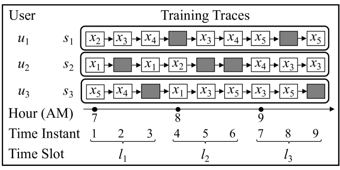
Figure 1: Training traces ($|\mathcal{U}|=3$, $|\mathcal{X}|=5$, $|\mathcal{T}|=9$, $|\mathcal{L}|=3$). Missing events are marked with gray.

2.1 Notations

Let $\mathbb{N}$, $\mathbb{Z}_{\geq 0}$, $\mathbb{R}$, and $\mathbb{R}_{\geq 0}$ be the set of natural numbers, non-negative integers, real numbers, and non-negative real numbers, respectively. For $n\in\mathbb{N}$, let $[n]=\{1,2,\cdots,n\}$. For a finite set $\mathcal{Z}$, let $\mathcal{Z}^{*}$ be the set of all finite sequences of elements of $\mathcal{Z}$. Let $\mathcal{P}(\mathcal{Z})$ be the power set of $\mathcal{Z}$.

We discretize locations by dividing the whole map into distinct regions or by extracting POIs. Let $\mathcal{X}$ be a finite set of discretized locations (i.e., regions or POIs). Let $x_{i}\in\mathcal{X}$ be the $i$-th location. We also discretize time into time instants (e.g., by rounding down minutes to a multiple of $20$, as in Figure 1), and represent a time instant as a natural number. Let $\mathcal{T}\subset\mathbb{N}$ be a finite set of time instants under consideration.

In addition to the time instant, we introduce a time slot as a time resolution in geo-data analysis; e.g., if we want to compute the time-dependent population distribution for every hour, then the length of each time slot is one hour. We represent a time slot as a set of time instants. Formally, let $\mathcal{L}\subseteq\mathcal{P}(\mathcal{T})$ be a finite set of time slots, and $l_{i}\in\mathcal{L}$ be the $i$-th time slot. Figure 1 shows an example of time slots, where $l_{1}=\{1,2,3\}$, $l_{2}=\{4,5,6\}$, $l_{3}=\{7,8,9\}$, and $\mathcal{L}=\{l_{1},l_{2},l_{3}\}$. The time slot can comprise either one time instant or multiple time instants (as in Figure 1). The time slot can also comprise separated time instants; e.g., if we set the interval between two time instants to $1$ hour, and want to average the population distribution for every two hours over two days, then $l_{1}=\{1,2,25,26\},l_{2}=\{3,4,27,28\},\cdots,l_{12}=\{23,24,47,48\}$, and $\mathcal{L}=\{l_{1},\cdots l_{12}\}$.

Next we formally define traces as described below. We refer to a pair of a location and a time instant as an event, and denote the set of all events by $\mathcal{E}=\mathcal{X}\times\mathcal{T}$. Let $\mathcal{U}$ be a finite set of all training users, and $u_{n}\in\mathcal{U}$ be the $n$-th training user. Then we define each trace as a pair of a user and a finite sequence of events, and denote the set of all traces by $\mathcal{R}=\mathcal{U}\times\mathcal{E}^{*}$. Each trace may be missing some events. Without loss of generality, we assume that each training user has provided a single training trace (if a user provides multiple temporally-separated traces, we can concatenate them into a single trace by regarding events between the traces as missing). Let $\mathcal{S}\subseteq\mathcal{R}$ be the finite set of all training traces, and $s_{n}\in\mathcal{S}$ be the $n$-th training trace (i.e., training trace of $u_{n}$). In Figure 1, $s_{1}=(u_{1},(x_{2},1),(x_{3},2),(x_{4},3),(x_{3},5),\allowbreak(x_{4},6),\allowbreak(x_{5},7),(x_{5},9))$ and $\mathcal{S}=\{s_{1},s_{2},s_{3}\}$.

We train parameters of a generative model (e.g., semantic clusters in SGLT [8], factor matrices in PPMTF) from training traces, and use the model to synthesize a trace. Since we want to preserve cluster-specific features, we assume a type of generative model in [8, 9] as described below. Let $y\in\mathcal{R}$ be a synthetic trace. For $n\in[|\mathcal{U}|]$, let $\mathcal{M}_{n}$ be a generative model of user $u_{n}$ that outputs a synthetic trace $y\in\mathcal{R}$ with probability $p(y=\mathcal{M}_{n})$. $\mathcal{M}_{n}$ is designed so that the synthetic trace $y$ (somewhat) resembles the training trace $s_{n}$ of $u_{n}$, while protecting the privacy of $u_{n}$. Let $\mathcal{M}$ be a probabilistic generative model that, given a user index $n\in[|\mathcal{U}|]$ as input, outputs a synthetic trace $y\in\mathcal{R}$ produced by $\mathcal{M}_{n}$; i.e., $p(y=\mathcal{M}(n))=p(y=\mathcal{M}_{n})$. $\mathcal{M}$ consists of $\mathcal{M}_{1},\cdots,\mathcal{M}_{|\mathcal{U}|}$, and the parameters of $\mathcal{M}_{1},\cdots,\mathcal{M}_{|\mathcal{U}|}$ are trained from training traces $\mathcal{S}$. A synthetic trace $y$ that resembles $s_{n}$ too much can violate the privacy of $u_{n}$, whereas it preserves a lot of features specific to clusters $u_{n}$ belongs to. Therefore, there is a trade-off between the cluster-specific features and user privacy. In Appendix C, we show an example of $\mathcal{M}_{n}$ in SGD [9].

In Appendix A, we also show tables summarizing the basic notations and abbreviations.

2.2 Privacy Metric

We explain PD (Plausible Deniability) [8, 9] as a privacy metric. The notion of PD was originally introduced by Bindschaedler and Shokri [8] to quantify how well a trace $y$ synthesized from a generative model $\mathcal{M}$ provides privacy for an input user $u_{n}$. However, PD in [8] was defined using a semantic distance between traces, and its relation with DP was unclear. Later, Bindschaedler et al. [9] modified PD to clarify the relation between PD and DP. In this paper, we use PD in [9]:

Definition 1 ($(k,\eta)$-PD).

Let $k\in\mathbb{N}$ and $\eta\in\mathbb{R}_{\geq 0}$. For a training trace set $\mathcal{S}$ with $|\mathcal{S}|\geq k$, a synthetic trace $y\in\mathcal{R}$ output by a generative model $\mathcal{M}$ with an input user index $d_{1}\in[|\mathcal{U}|]$ is releasable with $(k,\eta)$-PD if there exist at least $k-1$ distinct training user indexes $d_{2},\cdots,d_{k}\in[|\mathcal{U}|]\backslash\{d_{1}\}$ such that for any $i,j\in[k]$,

$$e^{\!-\eta}p(y{=}\mathcal{M}(d_{j}))\leq p(y{=}\mathcal{M}(d_{i}))\leq e^{\eta}p(y{=}\mathcal{M}(d_{j})).$$ (1)

The intuition behind $(k,\eta)$-PD can be explained as follows. Assume that user $u_{n}$ is an input user of the synthetic trace $y$. Since $y$ resembles the training trace $s_{n}$ of $u_{n}$, it would be natural to consider an adversary who attempts to recover $s_{n}$ (i.e., infer a pair of a user and the whole sequence of events in $s_{n}$) from $y$. This attack is called the tracking attack, and is decomposed into two phases: re-identification (or de-anonymization) and de-obfuscation [63]. The adversary first uncovers the fact that user $u_{n}$ is an input user of $y$, via re-identification. Then she infers events of $u_{n}$ via de-obfuscation. $(k,\eta)$-PD can prevent re-identification because it guarantees that the input user $u_{n}$ is indistinguishable from at least $k-1$ other training users. Then the tracking attack is prevented even if de-obfuscation is perfectly done. A large $k$ and a small $\eta$ are desirable for strong privacy.

$(k,\eta)$-PD can be used to alleviate the linkage of the input user $u_{n}$ and the synthetic trace $y$. However, $y$ may also leak information about parameters of the generative model $\mathcal{M}_{n}$ because $y$ is generated using $\mathcal{M}_{n}$. In Section 3.5, we discuss the overall privacy of PPMTF including this issue in detail.

3 Privacy-Preserving Multiple Tensor Factorization (PPMTF)

We propose PPMTF for synthesizing location traces. We first present an overview (Section 3.1). Then we explain the computation of two tensors (Section 3.2), the training of our generative model (Section 3.3), and the synthesis of traces (Section 3.4). Finally, we introduce the PD (Plausible Deniability) test (Section 3.5).

3.1 Overview

Proposed method.  Figure 2 shows an overview of PPMTF (we formally define the symbols that newly appear in Figure 2 in Sections 3.2 to 3.4). It comprises the following four steps.

1. We compute a transition-count tensor $\mathbf{R}^{\mathrm{I}}$ and visit-count tensor $\mathbf{R}^{\mathrm{II}}$ from a training trace set $\mathcal{S}$.

   The transition-count tensor $\mathbf{R}^{\mathrm{I}}$ comprises the “User,” “Location,” and “Next Location” modes. Its ($n,i,j$)-th element includes a transition-count of user $u_{n}\in\mathcal{U}$ from location $x_{i}\in\mathcal{X}$ to $x_{j}\in\mathcal{X}$. In other words, this tensor represents the movement pattern of each training user in the form of transition-counts. The visit-count tensor $\mathbf{R}^{\mathrm{II}}$ comprises the “User,” “Location,” and “Time Slot” modes. The ($n,i,j$)-th element includes a visit-count of user $u_{n}$ at location $x_{i}$ in time slot $l_{j}\in\mathcal{L}$. That is, this tensor includes a histogram of visited locations for each user and each time slot.

2. We factorize the two tensors $\mathbf{R}^{\mathrm{I}}$ and $\mathbf{R}^{\mathrm{II}}$ simultaneously via MTF (Multiple Tensor Factorization) [35, 66], which factorizes multiple tensors into low-rank matrices called factor matrices along each mode (axis). In MTF, one tensor shares a factor matrix from the same mode with other tensors.

   In our case, we factorize $\mathbf{R}^{\mathrm{I}}$ and $\mathbf{R}^{\mathrm{II}}$ into factor matrices $\mathbf{A}$, $\mathbf{B}$, $\mathbf{C}$, and $\mathbf{D}$, which respectively correspond to the “User,” “Location,” “Next Location,” and “Time Slot” mode. Here $\mathbf{A}$ and $\mathbf{B}$ are shared between the two tensors. $\mathbf{A}$, $\mathbf{B}$, $\mathbf{C}$, and $\mathbf{D}$ are parameters of our generative model, and therefore we call them the MTF parameters. Let $\Theta=(\mathbf{A},\mathbf{B},\mathbf{C},\mathbf{D})$ be the tuple of MTF parameters. We train MTF parameters $\Theta$ from the two tensors via posterior sampling [68], which samples $\Theta$ from its posterior distribution given $\mathbf{R}^{\mathrm{I}}$ and $\mathbf{R}^{\mathrm{II}}$.

   

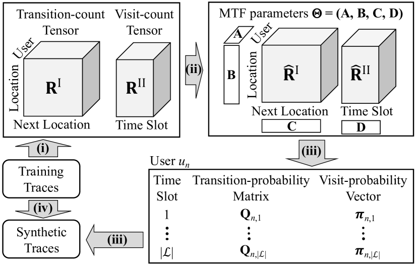
   Figure 2: Overview of PPMTF with the following four steps: (i) computing a transition-count tensor and visit-count tensor, (ii) training MTF parameters via posterior sampling, (iii) computing a transition-probability matrix and visit-probability vector via the MH algorithm and synthesizing traces, and (iv) the PD test.

3. We reconstruct two tensors from $\Theta$. Then, given an input user index $n\in[|\mathcal{U}|]$, we compute a transition-probability matrix $\mathbf{Q}_{n,i}$ and visit-probability vector $\pi_{n,i}$ of user $u_{n}\in\mathcal{U}$ for each time slot $l_{i}\in\mathcal{L}$. We compute them from the reconstructed tensors via the MH (Metropolis-Hastings) algorithm [50], which modifies the transition matrix so that $\pi_{n,i}$ is a stationary distribution of $\mathbf{Q}_{n,i}$. Then we generate a synthetic trace $y\in\mathcal{R}$ by using $\mathbf{Q}_{n,i}$ and $\pi_{n,i}$.

4. Finally, we perform the PD test [9], which verifies whether $y$ is releasable with $(k,\eta)$-PD.

We explain steps (i), (ii), (iii), and (iv) in Sections 3.2, 3.3, 3.4, and 3.5, respectively. We also explain how to tune hyperparameters (parameters to control the training process) in PPMTF in Section 3.5. Below we explain the utility, privacy, and scalability of PPMTF.

Utility.  PPMTF achieves high utility by modeling statistical features of training traces using two tensors. Specifically, the transition-count tensor represents the movement pattern of each user in the form of transition-counts, whereas the visit-count tensor includes a histogram of visited locations for each user and time slot. Consequently, our synthetic traces preserve a time-dependent population distribution, a transition matrix, and a distribution of visit-counts per location; i.e., features (a), (b), and (c) in Section 1.

Furthermore, PPMTF automatically finds a cluster of users who have similar behaviors (e.g., those who always stay in Manhattan; those who often visit universities) and locations that are semantically similar (e.g., restaurants and bars) because factor matrices in tensor factorization represent clusters [16]. Consequently, our synthetic traces preserve the mobility behavior of similar users and the semantics of similar locations. They also preserve a cluster-specific population distribution; i.e., feature (d) in Section 1,

More specifically, each column in $\mathbf{A}$, $\mathbf{B}$, $\mathbf{C}$, and $\mathbf{D}$ represents a user cluster, location cluster, location cluster, and time cluster, respectively. For example, elements with large values in the first column in $\mathbf{B}$, $\mathbf{C}$, and $\mathbf{D}$ may correspond to bars, bars, and night, respectively. Then elements with large values in the first column in $\mathbf{A}$ represent a cluster of users who go to bars at night.

In Section 4, we present visualization of some clusters, which can be divided into geographic clusters (e.g., north-eastern part of Tokyo) and semantic clusters (e.g., trains, malls, universities). Semantic annotation of POIs [19, 71] can also be used to automatically find what each cluster represents (i.e., semantic annotation of clusters).

PPMTF also addresses sparseness of the tensors by sharing $\mathbf{A}$ and $\mathbf{B}$ between the two tensors. It is shown in [66] that the utility is improved by sharing factor matrices between tensors, especially when one of two tensors is extremely sparse. In Appendix E, we also show that the utility is improved by sharing $\mathbf{A}$ and $\mathbf{B}$.

Privacy.  PPMTF uses the PD test in [9] to provide PD for a synthetic trace. In our experiments, we show that PPMTF provides $(k,\eta)$-PD for reasonable $k$ and $\eta$.

We also note that a posterior sampling-based Bayesian learning algorithm, which produces a sample from a posterior distribution with bounded log-likelihood, provides DP without additional noise [68]. Based on this, we sample $\Theta$ from a posterior distribution given $\mathbf{R}^{\mathrm{I}}$ and $\mathbf{R}^{\mathrm{II}}$ to provide DP for $\Theta$. However, the privacy budget $\varepsilon$ needs to be very large to achieve high utility in PPMTF. We discuss this issue in Appendix G.

Scalability.  Finally, PPMTF achieves much higher scalability than SGLT [8]. Specifically, the time complexity of [8] (semantic clustering) is $O(|\mathcal{U}|^{2}|\mathcal{X}|^{3}|\mathcal{L}|)$, which is very large for training traces with large $|\mathcal{U}|$ and $|\mathcal{X}|$. On the other hand, the time complexity of PPMTF is $O(|\mathcal{U}||\mathcal{X}|^{2}||\mathcal{L}|)$ (see Appendix B for details), which is much smaller than the synthesizer in [8]. In our experiments, we evaluate the run time and show that our method is applicable to much larger-scale training datasets than SGLT.

3.2 Computation of Two Tensors

We next explain details of how to compute two tensors from a training trace set $\mathcal{S}$ (i.e., step (i)).

Two tensors.  Figure 3 presents an example of the two tensors computed from the training traces in Figure 1.

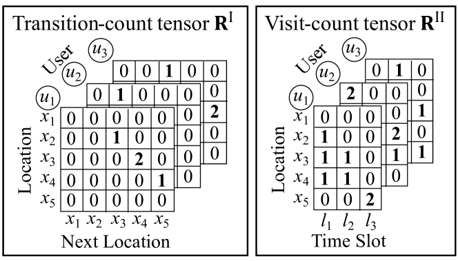
Figure 3: Two tensors obtained from the training traces in Figure 1.

The transition-count tensor includes a transition-count matrix for each user. Let $\mathbf{R}^{\mathrm{I}}\in\mathbb{Z}_{\geq 0}^{|\mathcal{U}|\times|\mathcal{X}|\times|\mathcal{X}|}$ be the transition-count tensor, and $r_{n,i,j}^{\mathrm{I}}\in\mathbb{Z}_{\geq 0}$ be its ($n,i,j$)-th element. For example, $r_{1,3,4}^{\mathrm{I}}=2$ in Figure 3 because two transitions from $x_{3}$ to $x_{4}$ are observed in $s_{1}$ of $u_{1}$ in Figure 1. The visit-count tensor includes a histogram of visited locations for each user and each time slot. Let $\mathbf{R}^{\mathrm{II}}\in\mathbb{Z}_{\geq 0}^{|\mathcal{U}|\times|\mathcal{X}|\times|\mathcal{L}|}$ be the visit-count tensor, and $r_{n,i,j}^{\mathrm{II}}\in\mathbb{Z}_{\geq 0}$ be its ($n,i,j$)-th element. For example, $r_{1,5,3}^{\mathrm{II}}=2$ in Figure 3 because $u_{1}$ visits $x_{5}$ twice in $l_{3}$ (i.e., from time instant $7$ to $9$) in Figure 1.

Let $\mathbf{R}=(\mathbf{R}^{\mathrm{I}},\mathbf{R}^{\mathrm{II}})$. Typically, $\mathbf{R}^{\mathrm{I}}$ and $\mathbf{R}^{\mathrm{II}}$ are sparse; i.e., many elements are zeros. In particular, $\mathbf{R}^{\mathrm{I}}$ can be extremely sparse because its size $|\mathbf{R}^{\mathrm{I}}|$ is quadratic in $|\mathcal{X}|$.

Trimming.  For both tensors, we randomly delete positive elements of users who have provided much more positive elements than the average (i.e., outliers) in the same way as [43]. This is called trimming, and is effective for matrix completion [34]. The trimming is also used to bound the log-likelihood in the posterior sampling method [43] (we also show in Appendix G that the log-likelihood is bounded by the trimming). Similarly, we set the maximum value of counts for each element, and truncate counts that exceed the maximum number.

Specifically, let $\lambda^{\mathrm{I}},\lambda^{\mathrm{II}}\in\mathbb{N}$ respectively represent the maximum numbers of positive elements per user in $\mathbf{R}^{\mathrm{I}}$ and $\mathbf{R}^{\mathrm{II}}$. Typically, $\lambda^{\mathrm{I}}\ll|\mathcal{X}|\times|\mathcal{X}|$ and $\lambda^{\mathrm{II}}\ll|\mathcal{X}|\times|\mathcal{L}|$. For each user, if the number of positive elements in $\mathbf{R}^{\mathrm{I}}$ exceeds $\lambda^{\mathrm{I}}$, then we randomly select $\lambda^{\mathrm{I}}$ elements from all positive elements, and delete the remaining positive elements. Similarly, we randomly delete extra positive elements in $\lambda^{\mathrm{II}}$. In addition, let $r_{max}^{\mathrm{I}},r_{max}^{\mathrm{II}}\in\mathbb{N}$ be the maximum counts for each element in $\mathbf{R}^{\mathrm{I}}$ and $\mathbf{R}^{\mathrm{II}}$, respectively. For each element, we truncate $r_{n,i,j}^{\mathrm{I}}$ to $r_{max}^{\mathrm{I}}$ if $r_{n,i,j}^{\mathrm{I}}>r_{max}^{\mathrm{I}}$ (resp. $r_{n,i,j}^{\mathrm{II}}$ to $r_{max}^{\mathrm{II}}$ if $r_{n,i,j}^{\mathrm{II}}>r_{max}^{\mathrm{II}}$).

In our experiments, we set $\lambda^{\mathrm{I}}=\lambda^{\mathrm{II}}=10^{2}$ (as in [43]) and $r_{max}^{\mathrm{I}}=r_{max}^{\mathrm{II}}=10$ because the number of positive elements per user and the value of counts were respectively less than $100$ and $10$ in most cases. In other words, the utility does not change much by increasing the values of $\lambda^{\mathrm{I}}$, $\lambda^{\mathrm{II}}$, $r_{max}^{\mathrm{I}}$, and $r_{max}^{\mathrm{II}}$. We also confirmed that much smaller values (e.g., $\lambda^{\mathrm{I}}=\lambda^{\mathrm{II}}=r_{max}^{\mathrm{I}}=r_{max}^{\mathrm{II}}=1$) result in a significant loss of utility.

3.3 Training MTF Parameters

After computing $\mathbf{R}=(\mathbf{R}^{\mathrm{I}},\mathbf{R}^{\mathrm{II}})$, we train the MTF parameters $\Theta=(\mathbf{A},\mathbf{B},\mathbf{C},\mathbf{D})$ via posterior sampling (i.e., step (ii)). Below we describe our MTF model and the training of $\Theta$.

Model.  Let $z\in\mathbb{N}$ be the number of columns (factors) in each factor matrix. Let $\mathbf{A}\in\mathbb{R}^{|\mathcal{U}|\times z}$, $\mathbf{B}\in\mathbb{R}^{|\mathcal{X}|\times z}$, $\mathbf{C}\in\mathbb{R}^{|\mathcal{X}|\times z}$, and $\mathbf{D}\in\mathbb{R}^{|\mathcal{L}|\times z}$ be the factor matrices. Typically, the number of columns is much smaller than the numbers of users and locations; i.e., $z\ll\min\{|\mathcal{U}|,|\mathcal{X}|\}$. In our experiments, we set $z=16$ as in [49] (we also changed the number $z$ of factors from $16$ to $32$ and confirmed that the utility was not changed much).

Let $a_{i,k},b_{i,k},c_{i,k},d_{i,k}\in\mathbb{R}$ be the $(i,k)$-th elements of $\mathbf{A}$, $\mathbf{B}$, $\mathbf{C}$, and $\mathbf{D}$, respectively. In addition, let $\hat{\mathbf{R}}^{\mathrm{I}}\in\mathbb{R}^{|\mathcal{U}|\times|\mathcal{X}|\times|\mathcal{X}|}$ and $\hat{\mathbf{R}}^{\mathrm{II}}\in\mathbb{R}^{|\mathcal{U}|\times|\mathcal{X}|\times|\mathcal{L}|}$ respectively represent two tensors that can be reconstructed from $\Theta$. Specifically, let $\hat{r}_{n,i,j}^{\mathrm{I}}\in\mathbb{R}$ and $\hat{r}_{n,i,j}^{\mathrm{II}}\in\mathbb{R}$ be the ($n,i,j$)-th elements of $\hat{\mathbf{R}}^{\mathrm{I}}$ and $\hat{\mathbf{R}}^{\mathrm{II}}$, respectively. Then $\hat{\mathbf{R}}^{\mathrm{I}}$ and $\hat{\mathbf{R}}^{\mathrm{II}}$ are given by:

$$\hat{r}_{n,i,j}^{\mathrm{I}}=\sum_{k\in[z]}a_{n,k}b_{i,k}c_{j,k},~{}\hat{r}_{n,i,j}^{\mathrm{II}}=\sum_{k\in[z]}a_{n,k}b_{i,k}d_{j,k},$$ (2)

where $\mathbf{A}$ and $\mathbf{B}$ are shared between $\hat{\mathbf{R}}^{\mathrm{I}}$ and $\hat{\mathbf{R}}^{\mathrm{II}}$.

For MTF parameters $\Theta$, we use a hierarchical Bayes model [59] because it outperforms the non-hierarchical one [58] in terms of the model’s predictive accuracy. Specifically, we use a hierarchical Bayes model shown in Figure 4. Below we explain this model in detail.

For the conditional distribution $p(\mathbf{R}|\Theta)$ of the two tensors $\mathbf{R}=(\mathbf{R}^{\mathrm{I}},\mathbf{R}^{\mathrm{II}})$ given the MTF parameters $\Theta=(\mathbf{A},\mathbf{B},\mathbf{C},\mathbf{D})$, we assume that each element $r_{n,i,j}^{\mathrm{I}}$ (resp. $r_{n,i,j}^{\mathrm{II}}$) is independently generated from a normal distribution with mean $\hat{r}_{n,i,j}^{\mathrm{I}}$ (resp. $\hat{r}_{n,i,j}^{\mathrm{II}}$) and precision (reciprocal of the variance) $\alpha\in\mathbb{R}_{\geq 0}$. In our experiments, we set $\alpha$ to various values from $10^{-6}$ to $10^{3}$.

Figure 4: Graphical model of PPMTF.

Here we randomly select a small number of zero elements in $\mathbf{R}$ to improve the scalability in the same way as [3, 54]. Specifically, we randomly select $\rho^{\mathrm{I}}\in\mathbb{N}$ and $\rho^{\mathrm{II}}\in\mathbb{N}$ zero elements for each user in $\mathbf{R}^{\mathrm{I}}$ and $\mathbf{R}^{\mathrm{II}}$, respectively, where $\rho^{\mathrm{I}}\ll|\mathcal{X}|\times|\mathcal{X}|$ and $\rho^{\mathrm{II}}\ll|\mathcal{X}|\times|\mathcal{L}|$ (in our experiments, we set $\rho^{\mathrm{I}}=\rho^{\mathrm{II}}=10^{3}$). We treat the remaining zero elements as missing. Let $I_{n,i,j}^{\mathrm{I}}$ (resp. $I_{n,i,j}^{\mathrm{II}}$) be the indicator function that takes $0$ if $r_{n,i,j}^{\mathrm{I}}$ (resp. $r_{n,i,j}^{\mathrm{II}}$) is missing, and takes $1$ otherwise. Note that $I_{n,i,j}^{\mathrm{I}}$ (resp. $I_{n,i,j}^{\mathrm{II}}$) takes 1 at most $\lambda^{\mathrm{I}}+\rho^{\mathrm{I}}$ (resp. $\lambda^{\mathrm{II}}+\rho^{\mathrm{II}}$) elements for each user, where $\lambda^{\mathrm{I}}$ (resp. $\lambda^{\mathrm{II}}$) is the maximum number of positive elements per user in $\mathbf{R}^{\mathrm{I}}$ (resp. $\mathbf{R}^{\mathrm{II}}$).

Then the distribution $p(\mathbf{R}|\Theta)$ can be written as:

$$\mathbin{\phantom{=}}p(\mathbf{R}|\Theta) =p(\mathbf{R}^{\mathrm{I}}|\mathbf{A},\mathbf{B},\mathbf{C})p(\mathbf{R}^{\mathrm{II}}|\mathbf{A},\mathbf{B},\mathbf{D})$$

$$=\mbox{\small$\displaystyle\prod_{n,i,j}$}[\mathcal{N}(r_{n,i,j}^{\mathrm{I}}|\hat{r}_{n,i,j}^{\mathrm{I}},\alpha^{\!-1})]^{I_{n,i,j}^{\mathrm{I}}}$$

$$\hskip 12.80373pt\cdot\mbox{\small$\displaystyle\prod_{n,i,j}$}[\mathcal{N}(r_{n,i,j}^{\mathrm{II}}|\hat{r}_{n,i,j}^{\mathrm{II}},\alpha^{\!-1})]^{I_{n,i,j}^{\mathrm{II}}},$$ (3)

where $\mathcal{N}(r|\mu,\alpha^{\!-1})$ denotes the probability of $r$ in the normal distribution with mean $\mu$ and precision $\alpha$ (i.e., variance $\alpha^{\!-1}$).

Let $\mathbf{a}_{i},\mathbf{b}_{i},\mathbf{c}_{i},\mathbf{d}_{i}\in\mathbb{R}^{z}$ be the $i$-th rows of $\mathbf{A}$, $\mathbf{B}$, $\mathbf{C}$, and $\mathbf{D}$, respectively. For a distribution of $\Theta=(\mathbf{A},\mathbf{B},\allowbreak\mathbf{C},\mathbf{D})$, we assume the multivariate normal distribution:

$$p(\mathbf{A}|\Psi_{\mathbf{A}}) =\textstyle\prod_{n}\mathcal{N}(\mathbf{a}_{n}|\mu_{\mathbf{A}},\Lambda_{\mathbf{A}}^{\!-1})$$

$$p(\mathbf{B}|\Psi_{\mathbf{B}}) =\textstyle\prod_{n}\mathcal{N}(\mathbf{b}_{n}|\mu_{\mathbf{B}},\Lambda_{\mathbf{B}}^{\!-1})$$

$$p(\mathbf{C}|\Psi_{\mathbf{C}}) =\textstyle\prod_{n}\mathcal{N}(\mathbf{c}_{n}|\mu_{\mathbf{C}},\Lambda_{\mathbf{C}}^{\!-1})$$

$$p(\mathbf{D}|\Psi_{\mathbf{D}}) =\textstyle\prod_{n}\mathcal{N}(\mathbf{d}_{n}|\mu_{\mathbf{D}},\Lambda_{\mathbf{D}}^{\!-1}),$$

where $\mu_{\mathbf{A}},$ $\mu_{\mathbf{B}}$, $\mu_{\mathbf{C}}$, $\mu_{\mathbf{D}}\in\mathbb{R}^{z}$ are mean vectors, $\Lambda_{\mathbf{A}}$, $\Lambda_{\mathbf{B}}$, $\Lambda_{\mathbf{C}}$, $\Lambda_{\mathbf{D}}\in\mathbb{R}^{z\times z}$ are precision matrices, and $\Psi_{\mathbf{A}}=(\mu_{\mathbf{A}},\Lambda_{\mathbf{A}})$, $\Psi_{\mathbf{B}}=(\mu_{\mathbf{B}},\Lambda_{\mathbf{B}})$, $\Psi_{\mathbf{C}}=(\mu_{\mathbf{C}},\Lambda_{\mathbf{C}})$, $\Psi_{\mathbf{D}}=(\mu_{\mathbf{D}},\Lambda_{\mathbf{D}})$.

The hierarchical Bayes model assumes a distribution for each of $\Psi_{\mathbf{A}}$, $\Psi_{\mathbf{B}}$, $\Psi_{\mathbf{C}}$, and $\Psi_{\mathbf{D}}$, which is called a hyperprior. We assume $\Psi_{\mathbf{Z}}\in\{\Psi_{\mathbf{A}},\Psi_{\mathbf{B}},\Psi_{\mathbf{C}},\Psi_{\mathbf{D}}\}$ follows a normal-Wishart distribution [10], i.e., the conjugate prior of a multivariate normal distribution:

$$p(\Psi_{\mathbf{Z}}) =p(\mu_{\mathbf{Z}}|\Lambda_{\mathbf{Z}})p(\Lambda_{\mathbf{Z}})$$

$$=\mathcal{N}(\mu_{\mathbf{Z}}|\mu_{0},(\beta_{0}\Lambda_{\mathbf{Z}})^{\!-1})\mathcal{W}(\Lambda_{\mathbf{Z}}|W_{0},\nu_{0}),$$ (4)

where $\mu_{0}\in\mathbb{R}^{z}$, $\beta_{0}\in\mathbb{R}$, and $\mathcal{W}(\Lambda|W_{0},\nu_{0})$ denotes the probability of $\Lambda\in\mathbb{R}^{z\times z}$ in the Wishart distribution with parameters $W_{0}\in\mathbb{R}^{z\times z}$ and $\nu_{0}\in\mathbb{R}$ ($W_{0}$ and $\nu_{0}$ represent the scale matrix and the number of degrees of freedom, respectively). $\mu_{0}$, $\beta_{0}$, $W_{0}$, and $\nu_{0}$ are parameters of the hyperpriors, and are determined in advance. In our experiments, we set $\mu_{0}=0$, $\beta_{0}=2$, $\nu_{0}=z$, and $W_{0}$ to the identity matrix, in the same way as [59].

Posterior sampling of $\Theta$.  We train $\Theta$ based on the posterior sampling method [68]. This method trains $\Theta$ from $\mathbf{R}$ by sampling $\Theta$ from the posterior distribution $p(\Theta|\mathbf{R})$. To sample $\Theta$ from $p(\Theta|\mathbf{R})$, we use Gibbs sampling [50], which samples each variable in turn, conditioned on the current values of the other variables.

Specifically, we sample $\Psi_{\mathbf{A}}$, $\Psi_{\mathbf{B}}$, $\Psi_{\mathbf{C}}$, $\Psi_{\mathbf{D}}$, $\mathbf{A}$, $\mathbf{B}$, $\mathbf{C}$, and $\mathbf{D}$ in turn. We add superscript “(t)” to these variables to denote the sampled values at the $t$-th iteration. For initial values with “(0)”, we use a random initialization method [4] that initializes each element as a random number in $[0,1]$ because it is widely used. Then, we sample $\Psi_{\mathbf{A}}^{(t)}$, $\Psi_{\mathbf{B}}^{(t)}$, $\Psi_{\mathbf{C}}^{(t)}$, $\Psi_{\mathbf{D}}^{(t)}$, $\mathbf{A}^{(t)}$, $\mathbf{B}^{(t)}$, $\mathbf{C}^{(t)}$, and $\mathbf{D}^{(t)}$ from the conditional distribution given the current values of the other variables, and iterate the sampling for a fixed number of times (see Appendix H for details of the sampling algorithm).

Gibbs sampling guarantees that the sampling distributions of $\mathbf{A}^{(t)},\cdots,\mathbf{D}^{(t)}$ approach the posterior distributions $p(\mathbf{A}|\mathbf{R}),\allowbreak\cdots,p(\mathbf{D}|\mathbf{R})$ as $t$ increases. Therefore, $\Theta^{(t)}=(\mathbf{A}^{(t)},\allowbreak\mathbf{B}^{(t)},\allowbreak\mathbf{C}^{(t)},\mathbf{D}^{(t)})$ approximates $\Theta$ sampled from the posterior distribution $p(\Theta|\mathbf{R})$ for large $t$. In our experiments, we discarded the first $99$ samples as “burn-in”, and used $\Theta^{(100)}$ as an approximation of $\Theta$. We also confirmed that the model’s predictive accuracy converged within $100$ iterations.

3.4 Generating Traces via MH

After training $\Theta=(\mathbf{A},\mathbf{B},\mathbf{C},\mathbf{D})$, we generate synthetic traces via the MH (Metropolis-Hastings) algorithm [50] (i.e., step (iii)). Specifically, given an input user index $n\in[|\mathcal{U}|]$, we generate a synthetic trace $y\in\mathcal{R}$ that resembles $s_{n}$ of user $u_{n}\in\mathcal{U}$ from $(\mathbf{a}_{n},\mathbf{B},\mathbf{C},\mathbf{D})$. In other words, the parameters of the generative model $\mathcal{M}_{n}$ of user $u_{n}$ are $(\mathbf{a}_{n},\mathbf{B},\mathbf{C},\mathbf{D})$.

Let $\mathcal{Q}$ be the set of $|\mathcal{X}|\times|\mathcal{X}|$ transition-probability matrices, and $\mathcal{C}$ be the set of $|\mathcal{X}|$-dimensional probability vectors (i.e., probability simplex). Given a transition-probability matrix $\mathbf{Q}\in\mathcal{Q}$ and a probability vector $\pi\in\mathcal{C}$, the MH algorithm modifies $\mathbf{Q}$ to $\mathbf{Q}^{\prime}\in\mathcal{Q}$ so that the stationary distribution of $\mathbf{Q}^{\prime}$ is equal to $\pi$. $\mathbf{Q}$ is a conditional distribution called a proposal distribution, and $\pi$ is called a target distribution.

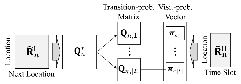
Figure 5: Computation of $(\mathbf{Q}_{n,i},\pi_{n,i})$ via MH. We compute $\mathbf{Q}_{n}^{*}$ from $\hat{\mathbf{R}}_{n}^{\mathrm{I}}$, and $\pi_{n,i}$ from $\hat{\mathbf{R}}_{n}^{\mathrm{II}}$. Then for each time slot $l_{i}\in\mathcal{L}$, we modify $\mathbf{Q}_{n}^{*}$ to $\mathbf{Q}_{n,i}$ whose stationary distribution is $\pi_{n,i}$.

In step (iii), given the input user index $n\in[|\mathcal{U}|]$, we reconstruct the transition-count matrix and visit-count matrix of user $u_{n}$, and use the MH algorithm to make a transition-probability matrix of $u_{n}$ consistent with a visit-probability vector of $u_{n}$ for each time slot. Figure 5 shows its overview. Specifically, let $\hat{\mathbf{R}}_{n}^{\mathrm{I}}\in\mathbb{R}^{|\mathcal{X}|\times|\mathcal{X}|}$ and $\hat{\mathbf{R}}_{n}^{\mathrm{II}}\in\mathbb{R}^{|\mathcal{X}|\times|\mathcal{L}|}$ be the $n$-th matrices in $\hat{\mathbf{R}}^{\mathrm{I}}$ and $\hat{\mathbf{R}}^{\mathrm{II}}$, respectively (i.e., reconstructed transition-count matrix and visit-count matrix of user $u_{n}$). We first compute $\hat{\mathbf{R}}_{n}^{\mathrm{I}}$ and $\hat{\mathbf{R}}_{n}^{\mathrm{II}}$ from $(\mathbf{a}_{n},\mathbf{B},\mathbf{C},\mathbf{D})$ by (2). Then we compute a transition-probability matrix $\mathbf{Q}_{n}^{*}\in\mathcal{Q}$ of user $u_{n}$ from $\hat{\mathbf{R}}_{n}^{\mathrm{I}}$ by normalizing counts to probabilities. Similarly, we compute a visit-probability vector $\pi_{n,i}\in\mathcal{C}$ of user $u_{n}$ for each time slot $l_{i}\in\mathcal{L}$ from $\hat{\mathbf{R}}_{n}^{\mathrm{II}}$ by normalizing counts to probabilities. Then, for each time slot $l_{i}\in\mathcal{L}$, we modify $\mathbf{Q}_{n}^{*}$ to $\mathbf{Q}_{n,i}\in\mathcal{Q}$ via the MH algorithm so that the stationary distribution of $\mathbf{Q}_{n,i}$ is equal to $\pi_{n,i}$. Then we generate a synthetic trace using $(\mathbf{Q}_{n,i},\pi_{n,i})$.

Below we explain step (iii) in more detail.

Computing $(\mathbf{Q}_{n,i},\pi_{n,i})$ via MH.  We first compute the $n$-th matrix $\hat{\mathbf{R}}_{n}^{\mathrm{I}}\in\mathbb{R}^{|\mathcal{X}|\times|\mathcal{X}|}$ in $\hat{\mathbf{R}}^{\mathrm{I}}$ from $\Theta$ by (2). Then we compute $\mathbf{Q}_{n}^{*}\in\mathcal{Q}$ from $\hat{\mathbf{R}}_{n}^{\mathrm{I}}$ by normalizing counts to probabilities as explained below. We assign a very small positive value $\phi\in\mathbb{R}_{\geq 0}$ ($\phi=10^{-8}$ in our experiments) to elements in $\hat{\mathbf{R}}_{n}^{\mathrm{I}}$ with values smaller than $\phi$. Then we normalize $\hat{\mathbf{R}}_{n}^{\mathrm{I}}$ to $\mathbf{Q}_{n}^{*}$ so that the sum over each row in $\mathbf{Q}_{n}^{*}$ is $1$. Since we assign $\phi$ ($=10^{-8}$) to elements with smaller values in $\hat{\mathbf{R}}_{n}^{\mathrm{I}}$, the transition-probability matrix $\mathbf{Q}_{n}^{*}$ is regular [50]; i.e., it is possible to get from any location to any location in one step. This allows $\pi_{n,i}$ to be the stationary distribution of $\mathbf{Q}_{n,i}$, as explained later in detail.

We then compute the $n$-th matrix $\hat{\mathbf{R}}_{n}^{\mathrm{II}}\in\mathbb{R}^{|\mathcal{X}|\times|\mathcal{L}|}$ in $\hat{\mathbf{R}}^{\mathrm{II}}$ from $\Theta$ by (2). For each time slot $l_{i}\in\mathcal{L}$, we assign $\phi$ ($=10^{-8}$) to elements with smaller values in $\hat{\mathbf{R}}_{n}^{\mathrm{II}}$. Then we normalize the $i$-th column of $\hat{\mathbf{R}}_{n}^{\mathrm{II}}$ to $\pi_{n,i}\in\mathcal{C}$ so that the sum of $\pi_{n,i}$ is one.

We use $\mathbf{Q}_{n}^{*}$ as a proposal distribution and $\pi_{n,i}$ as a target distribution, and apply the MH algorithm to obtain a transition-probability matrix $\mathbf{Q}_{n,i}$ whose stationary distribution is $\pi_{n,i}$. For $\mathbf{Q}\in\mathcal{Q}$ and $a,b\in[|\mathcal{X}|]$, we denote by $\mathbf{Q}(x_{b}|x_{a})\in[0,1]$ the transition probability from $x_{a}\in\mathcal{X}$ to $x_{b}\in\mathcal{X}$ (i.e., the $(a,b)$-th element of $\mathbf{Q}$). Similarly, given $\pi\in\mathcal{C}$, we denote by $\pi(x_{a})\in[0,1]$ the visit probability at $x_{a}\in\mathcal{X}$. Then, the MH algorithm computes $\mathbf{Q}_{n,i}(x_{b}|x_{a})$ for $x_{a}\neq x_{b}$ as follows:

$$\mathbf{Q}_{n,i}(x_{b}|x_{a})=\mathbf{Q}_{n}^{*}(x_{b}|x_{a})\min\big{(}1,{\textstyle\frac{\pi_{n,i}(x_{b})\mathbf{Q}_{n}^{*}(x_{a}|x_{b})}{\pi_{n,i}(x_{a})\mathbf{Q}_{n}^{*}(x_{b}|x_{a})}}\big{)},$$ (5)

and computes $\mathbf{Q}_{n,i}(x_{a}|x_{a})$ as follows: $\mathbf{Q}_{n,i}(x_{a}|x_{a})=1-\sum_{b\neq a}\mathbf{Q}_{n,i}(x_{b}|x_{a})$. Note that $\mathbf{Q}_{n,i}$ is regular because all elements in $\mathbf{Q}_{n}^{*}$ and $\pi_{n,i}$ are positive. Then the MH algorithm guarantees that $\pi_{n,i}$ is a stationary distribution of $\mathbf{Q}_{n,i}$ [50].

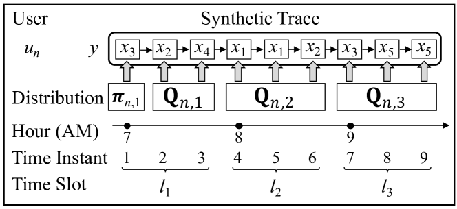
Figure 6: Generation of a synthetic trace ($|\mathcal{X}|=5$, $|\mathcal{T}|=9$, $|\mathcal{L}|=3$). Each location is randomly generated from a distribution in the same time slot.

Generating traces.  After computing $(\mathbf{Q}_{n,i},\pi_{n,i})$ via the MH algorithm, we synthesize a trace $y\in\mathcal{R}$ of user $u_{n}$ as follows. We randomly generate the first location in time slot $l_{1}$ from the visit-probability distribution $\pi_{n,1}$. Then we randomly generate the subsequent location in time slot $l_{i}$ using the transition-probability matrix $\mathbf{Q}_{n,i}$. Figure 6 shows an example of synthesizing a trace $y$ of user $u_{n}$. In this example, a location at time instant $7$ is randomly generated from the conditional distribution $\mathbf{Q}_{n,3}$ given the location $x_{2}$ at time instant $6$.

The synthetic trace $y$ is generated in such a way that a visit probability in time slot $l_{i}$ is given by $\pi_{n,i}$. In addition, the transition matrix is computed by using $\mathbf{Q}_{n}^{*}$ as a proposal distribution. Therefore, we can synthesize traces that preserve the statistical feature of training traces such as the time-dependent population distribution and the transition matrix.

3.5 Privacy Protection

We finally perform the PD test for a synthetic trace $y$.

Let $\mathcal{M}_{\textit{PPMTF}}$ be our generative model in step (iii) that, given an input user index $n\in[|\mathcal{U}|]$, outputs a synthetic trace $y\in\mathcal{R}$ with probability $p(y=\mathcal{M}_{\textit{PPMTF}}(n))$. Let $\sigma:\mathcal{T}\rightarrow\mathcal{X}$ be a function that, given time instant $t\in\mathcal{T}$, outputs an index of the location at time instant $t$ in $y$; e.g., $\sigma(1)=3,\sigma(2)=2,\cdots,\sigma(9)=5$ in Figure 6. Furthermore, let $\omega:\mathcal{T}\rightarrow\mathcal{L}$ be a function that, given time instant $t\in\mathcal{T}$, outputs an index of the corresponding time slot; e.g., $\omega(1)=\omega(2)=\omega(3)=1,\cdots,\omega(7)=\omega(8)=\omega(9)=3$ in Figure 6.

Recall that the first location in $y$ is randomly generated from $\pi_{n,1}$, and the subsequent location at time instant $t\in\mathcal{T}$ is randomly generated from $\mathbf{Q}_{n,\omega(t)}$. Then,

$$p(y=\mathcal{M}_{\textit{PPMTF}}(n))$$

$$=\pi_{n,1}(x_{\sigma(1)})\textstyle\prod_{t=2}^{|\mathcal{T}|}\mathbf{Q}_{n,\omega(t)}(x_{\sigma(t)}|x_{\sigma(t-1)}).$$

Thus, given $y\in\mathcal{R}$, we can compute $p(y=\mathcal{M}_{\textit{PPMTF}}(m))$ for any $m\in[|\mathcal{U}|]$ as follows: (i) compute $(\mathbf{Q}_{m,i},\pi_{m,i})$ for each time slot $l_{i}\in\mathcal{L}$ via the MH algorithm (as described in Section 3.4); (ii) compute $p(y=\mathcal{M}_{\textit{PPMTF}}(m))$ using $(\mathbf{Q}_{m,i},\pi_{m,i})$. Then we can verify whether $y$ is releasable with $(k,\eta)$-PD by counting the number of training users such that (1) holds.

Specifically, we use the following PD test in [9]:

Privacy Test 1 (Deterministic Test).

Let $k\in\mathbb{N}$ and $\eta\in\mathbb{R}_{\geq 0}$. Given a generative model $\mathcal{M}$, training user set $\mathcal{U}$, input user index $n\in[|\mathcal{U}|]$, and synthetic trace $y$, output pass or fail as follows:

1. Let $i\in\mathbb{Z}_{\geq 0}$ be a non-negative integer that satisfies:

   $$e^{-(i+1)\eta}<p(y=\mathcal{M}(n))\leq e^{-i\hskip 0.85358pt\eta}.$$ (6)

2. Let $k^{\prime}\in\mathbb{Z}_{\geq 0}$ be the number of training user indexes $m\in[|\mathcal{U}|]$ such that:

   $$e^{-(i+1)\eta}<p(y=\mathcal{M}(m))\leq e^{-i\hskip 0.85358pt\eta}.$$ (7)

3. If $k^{\prime}\geq k$, then return pass, otherwise return fail.

By (1), (6), and (7), if $y$ passes Privacy Test 1, then $y$ is releasable with $(k,\eta)$-PD. In addition, $(k,\eta)$-PD is guaranteed even if $\Theta$ is not sampled from the exact posterior distribution $p(\Theta|\mathbf{R})$.

The time complexity of Privacy Test 1 is linear in $|\mathcal{U}|$. In this paper, we randomly select a subset $\mathcal{U}^{*}\subseteq\mathcal{U}$ of training users from $\mathcal{U}$ (as in [9]) to ascertain more quickly whether $k^{\prime}\geq k$ or not. Specifically, we initialize $k^{\prime}$ to $0$, and check (7) for each training user in $\mathcal{U}^{*}\cup\{u_{n}\}$ (increment $k^{\prime}$ if (7) holds). If $k^{\prime}\geq k$, then we return pass (otherwise, return fail). The time complexity of this faster version of Privacy Test 1 is linear in $|\mathcal{U}^{*}|$ ($\leq|\mathcal{U}|$). A smaller $|\mathcal{U}^{*}|$ leads to a faster $(k,\eta)$-PD test at the expense of fewer synthetic traces passing the test.

In Section 4, we use the faster version of Privacy Test 1 with $|\mathcal{U}^{*}|=32000$, $k=10$ to $200$, and $\eta=1$ to guarantee $(k,\eta)$-PD for reasonable $k$ and $\eta$ (note that $\varepsilon=1$ is considered to be reasonable in $\varepsilon$-DP [23, 38]).

Overall privacy.  As described in Section 2.2, even if a synthetic trace $y$ satisfies $(k,\eta)$-PD, $y$ may leak information about the MTF parameters. We finally discuss the overall privacy of $y$ including this issue.

Given the input user index $n$, PPMTF generates $y$ from $(\mathbf{a}_{n},\mathbf{B},\mathbf{C},\mathbf{D})$, as described in Section 3.4. Since the linkage of the input user $u_{n}$ and $y$ is alleviated by PD, the leakage of $\mathbf{a}_{n}$ is also alleviated by PD. Therefore, the remaining issue is the leakage of $(\mathbf{B},\mathbf{C},\mathbf{D})$.

Here we note that $\mathbf{B}$ and $\mathbf{C}$ are information about locations (i.e., location profiles), and $\mathbf{D}$ is information about time (i.e., time profile). Thus, even if the adversary perfectly infers $(\mathbf{B},\mathbf{C},\mathbf{D})$ from $y$, it is hard to infer private information (i.e., training traces $\mathbf{S}$) of users $\mathcal{U}$ from $(\mathbf{B},\mathbf{C},\mathbf{D})$ (unless she obtains user profile $\mathbf{A}$). In fact, some studies on privacy-preserving matrix factorization [45, 53] release an item profile publicly. Similarly, SGLT [8] assumes that semantic clusters of locations (parameters of their generative model) leak almost no information about $\mathcal{U}$ because the location clusters are a kind of location profile. We also assume that the location and time profiles leak almost no information about users $\mathcal{U}$. Further analysis is left for future work.

Tuning hyperparameters.  As described in Sections 3.2, 3.3, and 3.5, we set $\lambda^{\mathrm{I}}=\lambda^{\mathrm{II}}=10^{2}$, $r_{max}^{\mathrm{I}}=r_{max}^{\mathrm{II}}=10$ (because the number of positive elements per user and the value of counts were respectively less than $100$ and $10$ in most cases), $z=16$ (as in [49]), $\rho^{\mathrm{I}}=\rho^{\mathrm{II}}=10^{3}$, $|\mathcal{U}^{*}|=32000$, and changed $\alpha$ from $10^{-6}$ and $10^{3}$ in our experiments. If we set these values to very small values, the utility is lost (we show its example by changing $\alpha$ in our experiments). For the parameters of the hyperpriors, we set $\mu_{0}=0$, $\beta_{0}=2$, $\nu_{0}=z$, and $W_{0}$ to the identity matrix in the same way as [59].

We set the hyperparameters as above based on the previous work or the datasets. To optimize the hyperparameters, we could use, for example, cross-validation [10], which assesses the hyperparameters by dividing a dataset into a training set and testing (validation) set.

4 Experimental Evaluation

In our experiments, we used two publicly available datasets: the SNS-based people flow data [52] and the Foursquare dataset in [69]. The former is a relatively small-scale dataset with no missing events. It is used to compare the proposed method with two state-of-the-art synthesizers [8, 9]. The latter is one of the largest publicly available location datasets; e.g., much larger than [14, 56, 70, 75]. Since the location synthesizer in [8] cannot be applied to this large-scale dataset (as shown in Section 4.4), we compare the proposed method with [9].

4.1 Datasets

SNS-based People Flow Data.  The SNS-based people flow data [52] (denoted by PF) includes artificial traces around the Tokyo metropolitan area. The traces were generated from real geo-tagged tweets by interpolating locations every five minutes using railway and road information [60].

We divided the Tokyo metropolitan area into $20\times 20$ regions; i.e., $|\mathcal{X}|=400$. Then we set the interval between two time instants to $20$ minutes, and extracted traces from 9:00 to 19:00 for $1000$ users (each user has a single trace comprising $30$ events). We also set time slots to $20$ minutes long from 9:00 to 19:00. In other words, we assumed that each time slot comprises one time instant; i.e., $|\mathcal{L}|=30$. We randomly divided the $1000$ traces into $500$ training traces and $500$ testing traces; i.e., $|\mathcal{U}|=500$. The training traces were used for training generative models and synthesizing traces. The testing traces were used for evaluating the utility.

Since the number of users is small in PF, we generated ten synthetic traces from each training trace (each synthetic trace is from 9:00 to 19:00) and averaged the utility and privacy results over the ten traces to stabilize the performance.

Foursquare Dataset.  The Foursquare dataset (Global-scale Check-in Dataset with User Social Networks) [69] (denoted by FS) includes $90048627$ real check-ins by $2733324$ users all over the world.

We selected six cities with numerous check-ins and with cultural diversity in the same way as [69]: Istanbul (IST), Jakarta (JK), New York City (NYC), Kuala Lumpur (KL), San Paulo (SP), and Tokyo (TKY). For each city, we extracted $1000$ POIs, for which the number of visits from all users was the largest; i.e., $|\mathcal{X}|=1000$. We set the interval between two time instants to $1$ hour (we rounded down minutes), and assigned every $2$ hours into one of $12$ time slots $l_{1}$ ($0$-$2$h), $\cdots$, $l_{12}$ ($22$-$24$h) in a cyclic manner; i.e., $|\mathcal{L}|=12$. For each city, we randomly selected $80\%$ of traces as training traces and used the remaining traces as testing traces. The numbers $|\mathcal{U}|$ of users in IST, JK, NYC, KL, SP, and TKY were $219793$, $83325$, $52432$, $51189$, $42100$, and $32056$, respectively. Note that there were many missing events in FS because FS is a location check-in dataset. The numbers of temporally-continuous events in the training traces of IST, JK, NYC, KL, SP, and TKY were $109027$, $19592$, $7471$, $25563$, $13151$, and $47956$, respectively.

From each training trace, we generated one synthetic trace with the length of one day.

4.2 Location Synthesizers

We evaluated the proposed method (PPMTF), the synthetic location traces generator in [8] (SGLT), and the synthetic data generator in [9] (SGD).

In PPMTF, we set $\lambda^{\mathrm{I}}=\lambda^{\mathrm{II}}=10^{2}$, $r_{max}^{\mathrm{I}}=r_{max}^{\mathrm{II}}=10$, $z=16$, $\rho^{\mathrm{I}}=\rho^{\mathrm{II}}=10^{3}$, $\mu_{0}=0$, $\beta_{0}=2$, $\nu_{0}=z$, and $W_{0}$ to the identity matrix, as explained in Section 3. Then we evaluated the utility and privacy for each value.

In SGLT [8], we used the SGLT tool (C++) in [7]. We set the location-removal probability $par_{c}$ to $0.25$, the location merging probability $par_{m}$ to $0.75$, and the randomization multiplication factor $par_{v}$ to $4$ in the same way as [8] (for details of the parameters in SGLT, see [8]). For the number $c$ of semantic clusters, we attempted various values: $c=50$, $100$, $150$, or $200$ (as shown later, SGLT provided the best performance when $c=50$ or $100$). For each case, we set the probability $par_{l}$ of removing the true location in the input user to various values from $0$ to $1$ ($par_{l}=1$ in [8]) to evaluate the trade-off between utility and privacy.

In SGD [9], we trained the transition matrix for each time slot ($|\mathcal{L}|\times|\mathcal{X}|\times|\mathcal{X}|$ elements in total) and the visit-probability vector for the first time instant ($|\mathcal{X}|$ elements in total) from the training traces via maximum likelihood estimation. Note that the transition matrix and the visit-probability vector are common to all users. Then we generated a synthetic trace from an input user by copying the first $\xi\in\mathbb{Z}_{\geq 0}$ events of the input user and generating the remaining events using the trained transition matrix. When $\xi=0$, we randomly generated a location at the first time instant using the visit-probability vector. For more details of SGD for location traces, see Appendix C. We implemented PPMTF and SGD with C++, and published it as open-source software [1].

4.3 Performance Metrics

Utility.  We evaluated the utility listed in Section 1.

(a) Time-dependent population distribution.  We computed a frequency distribution ($|\mathcal{X}|$-dim vector) of the testing traces and that of the synthetic traces for each time slot. Then we evaluated the average total variation between the two distributions over all time slots (denoted by TP-TV).

Frequently visited locations are especially important for some tasks [19, 76]. Therefore, for each time slot, we also selected the top $50$ locations, whose frequencies in the testing traces were the largest, and regarded the absolute error for the remaining locations in TP-TV as $0$ (TP-TV-Top50).

(b) Transition matrix.  We computed an average transition-probability matrix ($|\mathcal{X}|\times|\mathcal{X}|$ matrix) over all users and all time instances from the testing traces. Similarly, we computed an average transition-probability matrix from the synthetic traces.

Since each row of the transition matrix represents a conditional distribution, we evaluated the EMD (Earth Mover’s Distance) between the two conditional distributions over the $x$-axis (longitude) and $y$-axis (latitude), and averaged it over all rows (TM-EMD-X and TM-EMD-Y). TM-EMD-X and TM-EMD-Y represent how the two transition matrices differ over the $x$-axis and $y$-axis, respectively. They are large especially when one matrix allows only a transition between close locations and the other allows a transition between far-away locations (e.g., two countries). The EMD is also used in [8] to measure the difference in two transition matrices. We did not evaluate the two-dimensional EMD, because the computational cost of the EMD is expensive.

(c) Distribution of visit-fractions.  Since we used POIs in FS (regions in PF), we evaluated how well the synthetic traces preserve a distribution of visit-fractions in FS. We first excluded testing traces that have a few events (fewer than $5$). Then, for each of the remaining traces, we computed a fraction of visits for each POI. Based on this, we computed a distribution of visit-fractions for each POI by dividing the fraction into $24$ bins as $(0,\frac{1}{24}],(\frac{1}{24},\frac{2}{24}],\cdots,(\frac{23}{24},1)$. Similarly, we computed a distribution of visit-fractions for each POI from the synthetic traces. Finally, we evaluated the total variation between the two distributions (VF-TV).

(d) Cluster-specific population distribution.  To show that PPMTF is also effective in this respect, we conducted the following analysis. We used the fact that each column in the factor matrix $\mathbf{A}$ represents a cluster ($z=16$ clusters in total). Specifically, for each column in $\mathbf{A}$, we extracted the top $10\%$ users whose values in the column are the largest. These users form a cluster who exhibit similar behavior. For some clusters, we visualized factor matrices and the frequency distributions (i.e., cluster-specific population distributions) of the training traces and synthetic traces.

Privacy.  In PF, we evaluated the three synthesizers. Although PPMTF and SGD provide $(k,\eta)$-PD in Definition 1, SGLT provides PD using a semantic distance between traces [8], which differs from PD in Definition 1.

To compare the three synthesizers using the same privacy metrics, we considered two privacy attacks: re-identification (or de-anonymization) attack [63, 26, 47] and membership inference attack [62, 31]. In the re-identification attack, the adversary identifies, for each synthetic trace $y$, an input user of $y$ from $|\mathcal{U}|=500$ training users. We evaluated a re-identification rate as the proportion of correctly identified synthetic traces.

In the membership inference attack, the adversary obtains all synthetic traces. Then the adversary determines, for each of $1000$ users ($500$ training users and $500$ testing users), whether her trace is used for training the model. Here training users are members and testing users are non-members (they are randomly chosen, as described in Section 4.1). We used membership advantage [72] as a privacy metric in the same way as [31]. Specifically, let $tp$, $tn$, $fp$, and $fn$ be the number of true positives, true negatives, false positives, and false negatives, respectively, where “positive/negative” represents a member/non-member. Then membership advantage is defined in [72] as the difference between the true positive rate and the false positive rate; i.e., membership advantage $=\frac{tp}{tp+fn}-\frac{fp}{fp+tn}=\frac{tp-fp}{500}$. Note that membership advantage can be easily translated into membership inference accuracy, which is the proportion of correct adversary’s outputs ($=\frac{tp+tn}{tp+tn+fp+fn}=\frac{tp+tn}{1000}$), as follows: $\text{membership inference accuracy}=\frac{\text{membership advantage}+1}{2}$ (since $tn+fp=500$). A random guess that randomly outputs “member” with probability $q\in[0,1]$ achieves advantage $=0$ and accuracy $=0.5$.

For both the re-identification attack and membership inference attack, we assume the worst-case scenario about the background knowledge of the adversary; i.e., maximum-knowledge attacker model [20]. Specifically, we assumed that the adversary obtains the $1000$ original traces ($500$ training traces and $500$ testing traces) in PF. Note that the adversary does not know which ones are training traces (and therefore performs the membership inference attack). The adversary uses the $1000$ original traces to build an attack model. For a re-identification algorithm, we used the Bayesian re-identification algorithm in [47]. For a membership inference algorithm, we implemented a likelihood-ratio based membership inference algorithm, which partly uses the algorithm in [48]. For details of the attack algorithms, see Appendix D.

Note that evaluation might be difficult for a partial-knowledge attacker who has less background knowledge. In particular, when the amount of training data is small, it is very challenging to accurately train an attack model (transition matrices) [46, 48, 47]. We note, however, that if a location synthesizer is secure against the maximum-knowledge attacker, then we can say that it is also secure against the partial-knowledge attacker, without implementing clever attack algorithms. Therefore, we focus on the maximum-knowledge attacker model.

In FS, we used $(k,\eta)$-PD in Definition 1 as a privacy metric because we evaluated only PPMTF and SGD. As a PD test, we used the (faster) Privacy Test 1 with $|\mathcal{U}^{*}|=32000$, $k=10$ to $200$, and $\eta=1$.

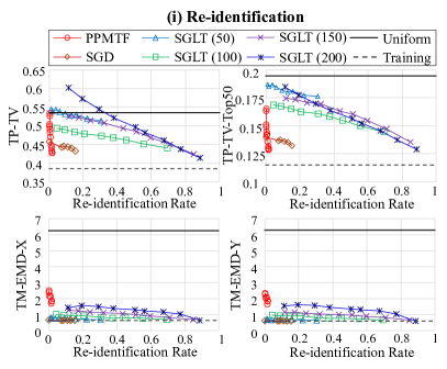
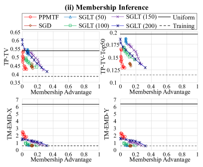
Figure 7: Privacy and utility in PF. The number in SGLT represents the number $c$ of clusters. In PPMTF, SGLT and SGD, we varied $\alpha$, $par_{l}$ and $\xi$, respectively. Lower is better in all of the utility metrics.

Scalability.  We measured the time to synthesize traces using the ABCI (AI Bridging Cloud Infrastructure) [51], which is a supercomputer ranking 8th in the Top 500 (as of June 2019). We used one computing node, which consists of two Intel Xeon Gold 6148 processors (2.40 GHz, 20 Cores) and 412 GB main memory.

4.4 Experimental Results in PF

Utility and privacy.  Figure 7 shows the re-identification rate, membership advantage, and utility with regard to (a) the time-dependent population distribution and (b) transition matrix in PF. Here, we set the precision $\alpha$ in PPMTF to various values from $0.5$ to $1000$. Uniform represents the utility when all locations in synthetic traces are independently sampled from a uniform distribution. Training represents the utility of the training traces; i.e., the utility when we output the training traces as synthetic traces without modification. Ideally, the utility of the synthetic traces should be much better than that of Uniform and close to that of Training.

Figure 7 shows that PPMTF achieves TP-TV and TP-TV-Top50 close to Training for while protecting user privacy. For example, PPMTF achieves TP-TV $=0.43$ and TP-TV-Top50 $=0.13$, both of which are close to those of Training (TP-TV $=0.39$ and TP-TV-Top50 $=0.12$), while keeping re-identification rate $<0.02$ and membership advantage $<0.055$ (membership inference accuracy $<0.53$). We consider that PPMTF achieved low membership advantage because (1) held for not only $k-1$ training users but testing users (non-members).

In SGLT and SGD, privacy rapidly gets worse with decrease in TP-TV and TP-TV-Top50. This is because both SGLT and SGD synthesize traces by copying over some events from the training traces. Specifically, SGLT (resp. SGD) increases the number of copied events by decreasing $par_{l}$ (resp. increasing $\xi$). Although a larger number of copied events result in a decrease of both TP-TV and TP-TV-Top50, they also result in the rapid increase of the re-identification rate. This result is consistent with the uniqueness of location data; e.g., only three locations are sufficient to uniquely characterize $80\%$ of the individuals among $1.5$ million people [18].

Figure 7 also shows that PPMTF performs worse than SGLT and SGD in terms of TM-EMD-X and TM-EMD-Y. This is because PPMTF modifies the transition matrix so that it is consistent with a visit-probability vector using the MH algorithm (SGLT and SGD do not modify the transition matrix). It should be noted, however, that PPMTF significantly outperforms Uniform with regard to TM-EMD-X and TM-EMD-Y. This means that PPMTF preserves the transition matrix well.

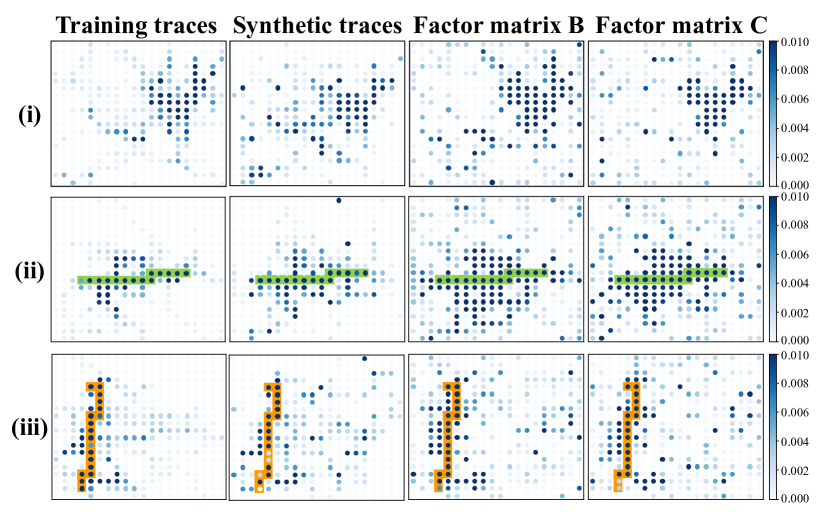
Figure 8: Frequency distributions and the columns of factor matrices $\mathbf{B}$ and $\mathbf{C}$ for three clusters ($50$ users for each cluster) in PF. The green line in (ii) and the orange line in (iii) represent subways (Shinjuku and Fukutoshin lines, respectively).

Analysis on cluster-specific features.  Next, we show the utility with regard to (d) the cluster-specific population distribution. Specifically, we show in Figure 8 the frequency distributions of training traces and synthetic traces and the columns of factor matrices B and C for three clusters (we set $\alpha=200$ because it provided almost the best utility in Figure 7; we also normalized elements in each column of B and C so that the square-sum is one). Recall that for each cluster, we extracted the top $10\%$ users; i.e., $50$ users.

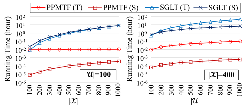
Figure 9: Running time in PF. “T” and “S” in the parentheses represent the time to train a generative model (i.e., MTF parameters in PPMTF and semantic clusters in SGLT) and the time to generate $500$ synthetic traces, respectively.

Figure 8 shows that the frequency distributions of training traces differ from cluster to cluster, and that the users in each cluster exhibit similar behavior; e.g., the users in (i) stay in the northeastern area of Tokyo; the users in (ii) and (iii) often use the subways. PPMTF models such a cluster-specific behavior via B and C, and synthesizes traces that preserve the behavior using B and C. Figure 8 shows that PPMTF is useful for geo-data analysis such as modeling human location patterns [40] and map inference [5, 41].

Scalability.  We also measured the time to synthesize traces from training traces. Here we generated one synthetic trace from each training trace ($500$ synthetic traces in total), and measured the time. We also changed the numbers of users and locations (i.e., $|\mathcal{U}|$, $|\mathcal{X}|$) for various values from $100$ to $1000$ to see how the running time depends on $|\mathcal{U}|$ and $|\mathcal{X}|$.

Figure 9 shows the results (we set $\alpha=200$ in PPMTF, and $c=100$ and $par_{l}=1$ in SGLT; we also obtained almost the same results for other values). Here we excluded the running time of SGD because it was very small; e.g., less than one second when $|\mathcal{U}|=1000$ and $|\mathcal{X}|=400$ (we compare the running time of PPMTF with that of SGD in FS, as described later). The running time of SGLT is much larger than that of PPMTF. Specifically, the running time of SGLT is quadratic in $|\mathcal{U}|$ (e.g., when $|\mathcal{X}|=400$, SGLT(T) requires $0.47$ and $47$ hours for $|\mathcal{U}|=100$ and $1000$, respectively) and cubic in $|\mathcal{X}|$ (e.g., when $|\mathcal{U}|=100$, SGLT(T) requires $8.1\times 10^{-3}$ and $8.4$ hours for $|\mathcal{X}|=100$ and $1000$, respectively). On the other hand, the running time of PPMTF is linear in $|\mathcal{U}|$ (e.g., PPMTF(S) requires $6.3\times 10^{-5}$ and $5.9\times 10^{-4}$ hours for $|\mathcal{U}|=100$ and $1000$, respectively) and quadratic in $|\mathcal{X}|$ (e.g., PPMTF(S) requires $9.3\times 10^{-3}$ and $0.96$ hours for $|\mathcal{X}|=100$ and $1000$, respectively). This is consistent with the time complexity described in Section 3.1.

From Figure 9, we can estimate the running time of SGLT for generating large-scale traces. Specifically, when $|\mathcal{U}|=219793$ and $|\mathcal{X}|=1000$ as in IST of FS, SGLT(T) (semantic clustering) would require about 4632 years (=$8.4\times(219793/\allowbreak 100)^{2}/(365\times 24)$). Even if we use $1000$ nodes of the ABCI (which has $1088$ nodes [51]) in parallel, SGLT(T) would require more than four years. Consequently, SGLT cannot be applied to IST. Therefore, we compare PPMTF with SGD in FS.

4.5 Experimental Results in FS

Utility and privacy.  In FS, we set $\alpha=200$ in PPMTF (as in Figures 8 and 9). In SGD, we set $\xi=0$ for the following two reasons: (1) the re-identification rate is high for $\xi\geq 1$ in Figure 7 because of the uniqueness of location data [18]; (2) the event in the first time slot is missing for many users in FS, and cannot be copied. Note that SGD with $\xi=0$ always passes the PD test because it generates synthetic traces independently of the input data record [9]. We evaluated all the utility metrics for PPMTF and SGD.

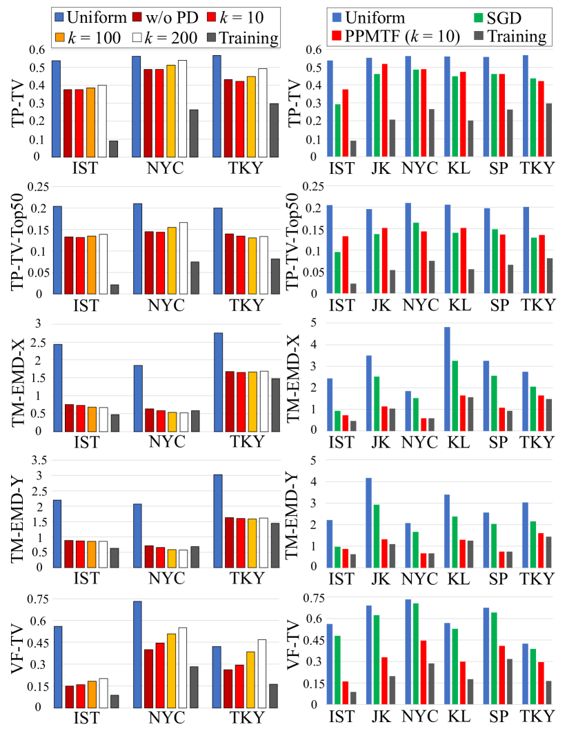
Figure 10: Utility of synthetic traces with $(k,1)$-PD in FS. The left graphs show the utility of PPMTF without the PD test, with $k=10$, $100$ or $200$. Lower is better in all of the utility metrics.

Figure 10 shows the results. The left graphs show PPMTF without the PD test, with $k=10$, $100$, or $200$ in IST, NYC, and TKY (we confirmed that the results of the other cities were similar to those of NYC and TKY). The right graphs show PPMTF with $k=10$ and SGD.

The left graphs show that all of the utility metrics are minimally affected by running the PD test with $k=10$ in all of the cities. Similarly, all of the utility metrics are minimally affected in IST, even when $k=200$. We confirmed that about $70\%$ of the synthetic traces passed the PD test when $k=10$, whereas only about $20\%$ of the synthetic traces passed the PD test when $k=200$ (see Appendix F for details). Nevertheless, PPMTF significantly outperforms Uniform in IST. This is because the number of users is very large in IST ($|\mathcal{U}|=219793$). Consequently, even if the PD test pass rate is low, many synthetic traces still pass the test and preserve various statistical features. Thus PPMTF achieves high utility especially for a large-scale dataset.

The right graphs in Figure 10 show that for TP-TV and TP-TV-Top50, PPMTF is roughly the same as SGD. For TM-EMD-X and TM-EMD-Y, PPMTF outperforms SGD, especially in JK, NYC, KL, and SP. This is because many missing events exist in FS and the transitions in the training traces are few in JK, NYC, KL, and SP (as described in Section 4.1).

A crucial difference between PPMTF and SGD lies in the fact that PPMTF models the cluster-specific mobility features (i.e., both (c) and (d)), whereas SGD ($\xi=0$) does not. This causes the results of VF-TV in Figure 10. Specifically, for VF-TV, SGD performs almost the same as Uniform, whereas PPMTF significantly outperforms SGD. Below we perform more detailed analysis to show how well PPMTF provides (c) and (d).

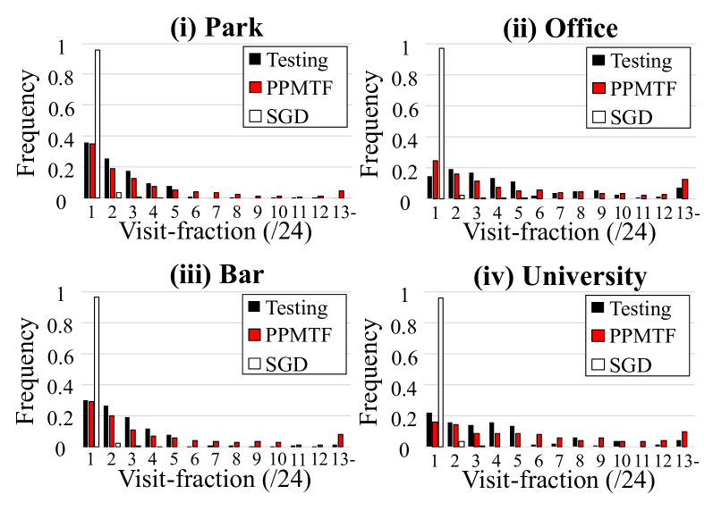
Figure 11: Distributions of visit-fractions in NYC. PPMTF provides $(10,1)$-PD.

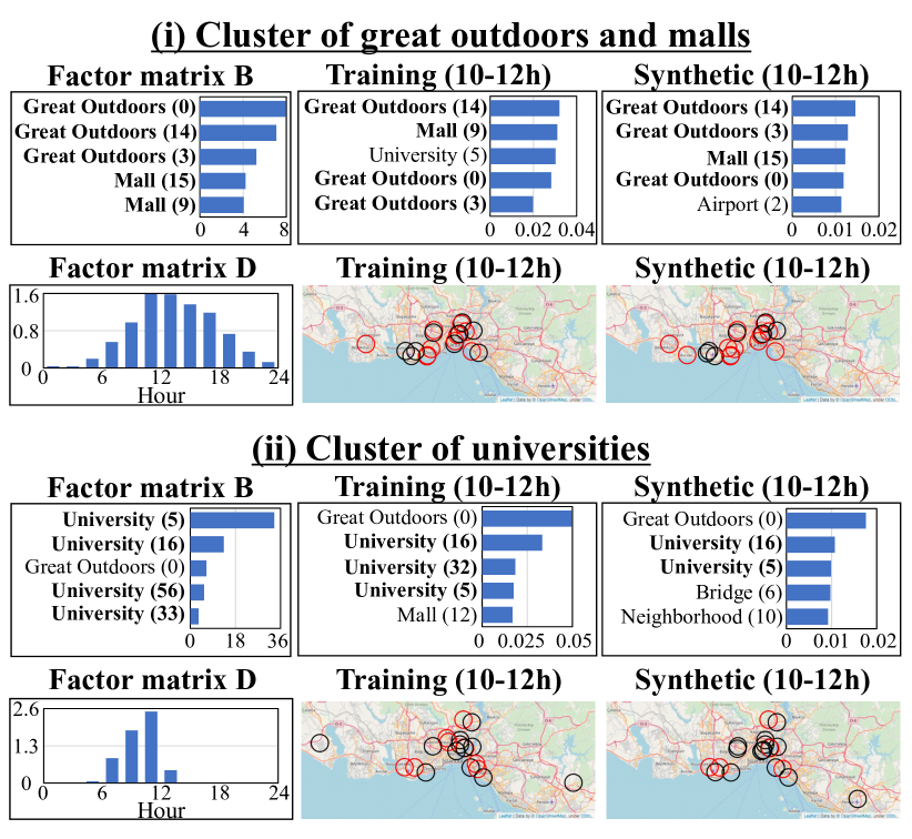
Figure 12: Two clusters in IST ($21980$ users for each cluster). Here PPMTF provides ($10,1$)-PD. For B and training/synthetic traces, we show the top $5$ POIs (numbers in parentheses represent POI IDs), whose values or frequencies from 10:00 to 12:00 are the highest. We show the top $20$ POIs by circles in the map. Red circles in (i) (resp. (ii)) represent outdoors/malls (resp. universities).

Analysis on cluster-specific features.  First, we show in Figure 11 the distributions of visit-fractions for four POI categories in NYC (Testing represents the distribution of testing traces). The distribution of SGD concentrates at the visit-fraction of $1/24$ (i.e., $0$ to $0.042$). This is because SGD ($\xi=0$) uses the transition matrix and visit-probability vector common to all users, and synthesizes traces independently of input users. Consequently, all users spend almost the same amount of time on each POI category. On the other hand, PPMTF models a histogram of visited locations for each user via the visit-count tensor, and generates traces based on the tensor. As a result, the distribution of PPMTF is similar to that of Testing, and reflects the fact that about $30$ to $35\%$ of users spend less than $1/24$ of their time at a park or bar, whereas about $80\%$ of users spend more than $1/24$ of their time at an office or university. This result explains the low values of VF-TV in PPMTF. Figure 11 also shows that PPMTF is useful for semantic annotation of POIs [19, 71].

Next, we visualize in Figure 12 the columns of factor matrices B and D and training/synthetic traces for two clusters. As with PF, the training users in each cluster exhibit a similar behavior; e.g., the users in (i) enjoy great outdoors and shopping at a mall, whereas the users in (ii) go to universities. Note that users and POIs in each cluster are semantically similar; e.g., people who enjoy great outdoors also enjoy shopping at a mall; many users in (ii) would be students, faculty, or staff. The activity times are also different between the two clusters. For example, we confirmed that many training users in (i) enjoy great outdoors and shopping from morning until night, whereas most training users in (ii) are not at universities at night. PPMTF models such a behavior via factor matrices, and synthesizes traces preserving the behavior. We emphasize that this feature is useful for various analysis; e.g., modeling human location patterns, semantic annotation of POIs.

SGD ($\xi=0$) and others [12, 13, 28] do not provide such cluster-specific features because they generate traces only based on parameters common to all users.

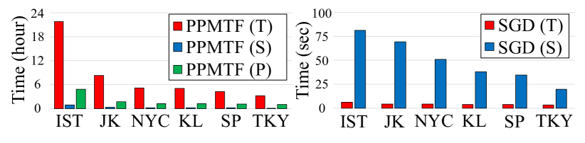
Figure 13: Running time in FS. “T”, “S”, and “P” represent the time to train a generative model, synthesize traces, and run the PD test, respectively.

Scalability.  Figure 13 shows the running time in FS. SGD is much faster than PPMTF. The reason for this lies in the simplicity of SGD; i.e., SGD trains a transition matrix for each time slot via maximum likelihood estimation; it then synthesizes traces using the transition matrix. However, SGD does not generate cluster-specific traces. To generate such traces, PPMTF is necessary.

Note that even though we used a supercomputer in our experiments, we used a single node and did not parallelize the process. We can also run PPMTF on a regular computer with large memory. For example, assume that we use $8$ bytes to store a real number, and that we want to synthesize all of $219793$ traces in IST. Then, $8|\mathcal{U}|(\lambda^{\mathrm{I}}+\rho^{\mathrm{I}}+\lambda^{\mathrm{II}}+\rho^{\mathrm{II}})+8z(|\mathcal{U}|+2|\mathcal{X}|+|\mathcal{L}|)=3.9$ GB memory is required to perform MTF, and the other processes need less memory. PPMTF could also be parallelized by using asynchronous Gibbs sampling [67].

5 Conclusion

In this paper, we proposed PPMTF (Privacy-Preserving Multiple Tensor Factorization), a location synthesizer that preserves various statistical features, protects user privacy, and synthesizes large-scale location traces in practical time. Our experimental results showed that PPMTF significantly outperforms two state-of-the-art location synthesizers [8, 9] in terms of utility and scalability at the same level of privacy.

We assumed a scenario where parameters of the generative model are kept secret (or discarded after synthesizing traces). As future work, we would like to design a location synthesizer that provides strong privacy guarantees in a scenario where the parameters of the generative model are made public. For example, one possibility might be to release only parameters $(\mathbf{B},\mathbf{C},\mathbf{D})$ (i.e., location and time profiles) and randomly generate $\mathbf{A}$ (i.e., user profile) from some distribution. We would like to investigate how much this approach can reduce $\varepsilon$ in DP.

Appendix A Notations and Abbreviations

Tables 1 and 2 respectively show the basic notations and abbreviations used in this paper.

Table 1: Basic notations in this paper ($\dagger$ represents $\mathrm{I}$ or $\mathrm{II}$).

Symbol Description $\mathcal{U}$ Finite set of training users. $\mathcal{X}$ Finite set of locations. $\mathcal{T}$ Finite set of time instants over $\mathbb{N}$. $\mathcal{L}$ Finite set of time slots ($\mathcal{L}\subseteq\mathcal{P}(\mathcal{T})$). $\mathcal{E}$ Finite set of events ($\mathcal{E}=\mathcal{X}\times\mathcal{T}$). $\mathcal{R}$ Finite set of traces ($\mathcal{R}=\mathcal{U}\times\mathcal{E}^{*}$). $\mathcal{S}$ Finite set of training traces ($\mathcal{S}\subseteq\mathcal{R}$). $\mathcal{F}$ Randomized algorithm with domain $\mathcal{P}(\mathcal{R})$. $\mathcal{M}$ Generative model. $u_{n}$ $n$-th training user ($u_{n}\in\mathcal{U}$). $x_{i}$ $i$-th location ($x_{i}\in\mathcal{X}$). $s_{n}$ $n$-th training trace ($s_{n}\in\mathcal{S}$). $y$ Synthetic trace ($y\in\mathcal{R}$). $\mathbf{R}$ Tuple of two tensors ($\mathbf{R}=(\mathbf{R}^{\mathrm{I}},\mathbf{R}^{\mathrm{II}})$). $\hat{\mathbf{R}}^{\dagger}$ Reconstructed tensors by $\Theta$. $r_{n,i,j}^{\dagger}$ ($n,i,j$)-th element of $\mathbf{R}^{\dagger}$. $\hat{r}_{n,i,j}^{\dagger}$ ($n,i,j$)-th element of $\hat{\mathbf{R}}^{\dagger}$. $\Theta$ Tuple of MTF parameters ($\Theta=(\mathbf{A},\mathbf{B},\mathbf{C},\mathbf{D})$). $z$ Number of columns in each factor matrix. $\mathcal{F}_{\textit{PPMTF}}$ Proposed training algorithm. $\mathcal{M}_{\textit{PPMTF}}$ Proposed generative model. $\mathbf{Q}_{n,i}$ Transition-probability matrix of user $u_{n}$ for time slot $l_{i}$ in $\mathcal{M}_{\textit{PPMTF}}$. $\pi_{n,i}$ Visit-probability vector of user $u_{n}$ for time slot $l_{i}$ in $\mathcal{M}_{\textit{PPMTF}}$. $\lambda^{\dagger}$ Maximum number of positive elements per user in $\mathbf{R}^{\dagger}$. $\rho^{\dagger}$ Number of selected zero elements per user in $\mathbf{R}^{\dagger}$. $r_{max}^{\dagger}$ Maximum value of counts for each element in $\mathbf{R}^{\dagger}$. $I_{n,i,j}^{\dagger}$ Indicator function that takes $0$ if $r_{n,i,j}^{\dagger}$ is missing, and takes $1$ otherwise.

Table 2: Abbreviations in this paper.

Abbreviation Description PPMTF Proposed location traces generator. SGLT Synthetic location traces generator in [8]. SGD Synthetic data generator in [9]. PF SNS-based people flow data [52]. FS Foursquare dataset [69]. IST/JK/NYC/ Istanbul/Jakarta/New York City/ KL/SP/TKY Kuala Lumpur/San Paulo/Tokyo. TP-TV(-Top50) Average total variation between time- dependent population distributions (over $50$ frequently visited locations). TM-EMD-X/Y Earth Mover’s Distance between transition- probability matrices over the $x$/$y$-axis. VF-TV Total variation between distributions of visit-fractions.

Appendix B Time Complexity

Assume that we generate a synthetic trace from each training trace $s_{n}\in\mathcal{S}$ (i.e., $|\mathcal{U}|$ synthetic traces in total). Assume that $\lambda^{\mathrm{I}}$, $\rho^{\mathrm{I}}$, $\lambda^{\mathrm{II}}$, $\rho^{\mathrm{II}}$, $z$, and $|\mathcal{U}^{*}|$ are constants.

In step (i), we simply count the number of transitions and the number of visits from a training trace set $\mathcal{S}$. Consequently, the computation time of this step is much smaller than that of the remaining three steps.

In step (ii), we first randomly select $\rho^{\mathrm{I}}$ and $\rho^{\mathrm{II}}$ zero elements for each user in $\mathbf{R}^{\mathrm{I}}$ and $\mathbf{R}^{\mathrm{II}}$, respectively. This can be done in $O(|\mathcal{U}|)$ time in total by using a sampling technique in [25]. Subsequently, we train the MTF parameters $\Theta$ via Gibbs sampling. The computation time of Gibbs sampling can be expressed as $O(|\mathcal{U}|+|\mathcal{X}|+|\mathcal{L}|)$.

In step (iii), we generate synthetic traces via the MH algorithm. This is dominated by computation of the transition-probability matrices $\mathbf{Q}_{n}^{*}$, $\mathbf{Q}_{n,1},\cdots,\mathbf{Q}_{n,|\mathcal{L}|}$ for each training trace $s_{n}$, which takes $O(|\mathcal{U}||\mathcal{X}|^{2}|\mathcal{L}|)$ time in total. Then we generate a synthetic trace $y$, which takes $O(|\mathcal{U}||\mathcal{X}||\mathcal{L}|)$ time.

In step (iv), the faster version of Privacy Test 1 in Section 3.5 computes the transition-probability matrices $\mathbf{Q}_{m}^{*}$, $\mathbf{Q}_{m,1},\cdots,\mathbf{Q}_{m,|\mathcal{L}|}$ for each training trace $s_{m}\in\mathcal{S}^{*}$, which takes $O(|\mathcal{X}|^{2}|\mathcal{L}|)$ time in total. Subsequently, we check whether $k^{\prime}\geq k$ for each training trace $s_{n}\in\mathcal{S}$, which takes $O(|\mathcal{U}||\mathcal{X}||\mathcal{L}|)$ time in total.

In summary, the time complexity of the proposed method can be expressed as $O(|\mathcal{U}||\mathcal{X}|^{2}|\mathcal{L}|)$.

Appendix C Details on SGD

SGD [9] is a synthetic generator for any kind of data, which works as follows: (i) Train the dependency structure (graph) between data attributes; (ii) Train conditional probabilities for each attribute given its parent attributes; (iii) Generate a synthetic data record from an input data record by copying the top $\gamma\in\mathbb{Z}_{\geq 0}$ attributes from the input data record and generating the remaining attributes using the trained conditional probabilities. Note that the dependency structure and the conditional probabilities are common to all users.

We applied SGD to synthesis of location traces as follows. We regarded an event as an attribute, and a location trace of length $|\mathcal{T}|$ as a data record with $|\mathcal{T}|$ attributes. Then it would be natural to consider that the dependency structure is given by the time-dependent Markov chain model as in PPMTF and SGLT, and the conditional probabilities are given by the transition matrix for each time slot. In other words, we need not train the dependency structure; i.e., we can skip (i).

We trained the transition matrix $\tilde{\mathbf{Q}}_{i}\in\mathcal{Q}$ for each time slot $l_{i}\in\mathcal{L}$ ($|\mathcal{L}|\times|\mathcal{X}|\times|\mathcal{X}|$ elements in total) and the visit-probability vector $\tilde{\pi}\in\mathcal{C}$ for the first time instant ($|\mathcal{X}|$ elements in total) from the training traces via maximum likelihood estimation. Then we synthesized a trace from an input user $u_{n}$ by copying the first $\gamma$ events in the training trace $s_{n}$ of $u_{n}$ and by generating the remaining events using the transition matrix. When $\gamma=0$, we generated a location at the first time instant using the visit-probability vector. Thus the parameters of the generative model $\mathcal{M}_{n}$ of user $u_{n}$ can be expressed as: $(\tilde{\mathbf{Q}}_{1},\cdots,\tilde{\mathbf{Q}}_{|\mathcal{L}|},\tilde{\pi},s_{n}$).

SGD can provide $(\varepsilon,\delta)$-DP for one synthetic trace $y$ by using a randomized test [9], which randomly selects an input user $u_{n}$ from $\mathcal{U}$ and adds the Laplacian noise to the parameter $k$ in $(k,\eta)$-PD. However, both $\varepsilon$ and $\delta$ can be large for multiple synthetic traces generated from the same input user, as discussed in [9]. Thus we did not use the randomized test in our experiments.

Appendix D Details on Privacy Attacks

Re-identification algorithm.  We used the Bayesian re-identification algorithm in [47]. Specifically, we first trained the transition matrix for each training user from the training traces via maximum likelihood estimation. Then we re-identified each synthetic trace $y$ by selecting a training user whose posterior probability of being the input user is the highest. Here we computed the posterior probability by calculating a likelihood for each training user and assuming a uniform prior for users. We calculated the likelihood by simply calculating a likelihood for each transition in $y$ using the transition matrix and multiplying them. We assigned a small positive value ($=10^{-8}$) to zero elements in the transition matrix so that the likelihood never becomes $0$.

Membership inference algorithm.  We considered a likelihood ratio-based membership inference algorithm, which partly uses the algorithm in [48] as follows.

Let $\mathcal{V}$ be a finite set of all training and testing users (each of them is either a member or a non-member; $|\mathcal{V}|=1000$ in PF), and $v_{n}\in\mathcal{V}$ be the $n$-th user. Assume that the adversary attempts to determine whether user $v_{n}$ is a training user (i.e., member) or not. Since each training user is used as an input user to generate a synthetic trace, the adversary can perform the membership inference by determining, for each synthetic trace $y$, whether $v_{n}$ is used as an input user to generate $y$. To perform this two-class classification (i.e., $v_{n}$ is an input user of $y$ or not), we used the likelihood ratio-based two-class classification algorithm in [48].

Specifically, given user $v_{n}$ and synthetic trace $y$, let $H_{1}$ (resp. $H_{0}$) be the hypothesis that $v_{n}$ is (resp. is not) an input user of $y$. We first trained the transition matrix for each of $|\mathcal{V}|=1000$ users from her (original) trace. Let $\mathbf{W}_{n}$ be the transition matrix of user $v_{n}$. We calculated a population transition matrix $\mathbf{W}_{0}$, which models the average behavior of users other than $v_{n}$ as the average of $\mathbf{W}_{m}$ ($m\neq n$); i.e., $\mathbf{W}_{0}=\frac{1}{|\mathcal{V}|-1}\sum_{m\neq n}\mathbf{W}_{m}$. Let $z_{1}$ (resp. $z_{0}$) $\in\mathbb{R}$ be the likelihood of $y$ given $H_{1}$ (resp. $H_{0}$). We calculated $z_{1}$ (resp. $z_{0}$) simply by calculating a likelihood for each transition in $y$ using the transition matrix $\mathbf{W}_{n}$ (resp. $\mathbf{W}_{0}$) and multiplying them (as in the re-identification attack). Then we compared the log-likelihood ratio $\log\frac{z_{1}}{z_{0}}$ with a threshold $\psi\in\mathbb{R}$. If $\log\frac{z_{1}}{z_{0}}\geq\psi$, we accepted $H_{1}$; otherwise, we accepted $H_{0}$.

We performed this two-class classification for each synthetic trace $y$. If we accepted $H_{1}$ for at least one synthetic trace $y$, then we decided that $v_{n}$ is a member. Otherwise, we decided that $v_{n}$ is a non-member.

In our experiments, we changed the threshold $\psi$ to various values. Then we evaluated, for each location synthesizer, the maximum membership advantage over the various thresholds (Figure 8 shows the results).

Appendix E Effect of Sharing A and B

The proposed method (PPMTF) shares the factor matrices A and B between two tensors. Here we show the effects of sharing them. Specifically, we compare the proposed method with a method that independently factorizes each tensor; i.e., factorizes $\mathbf{R}^{\mathrm{I}}$ into factor matrices $\mathbf{A}^{\mathrm{I}}\in\mathbb{R}^{|\mathcal{U}|\times z}$, $\mathbf{B}^{\mathrm{I}}\in\mathbb{R}^{|\mathcal{X}|\times z}$, $\mathbf{C}^{\mathrm{I}}\in\mathbb{R}^{|\mathcal{X}|\times z}$, and $\mathbf{R}^{\mathrm{II}}$ into factor matrices $\mathbf{A}^{\mathrm{II}}\in\mathbb{R}^{|\mathcal{U}|\times z}$, $\mathbf{B}^{\mathrm{II}}\in\mathbb{R}^{|\mathcal{X}|\times z}$, $\mathbf{D}^{\mathrm{II}}\in\mathbb{R}^{|\mathcal{L}|\times z}$, respectively. We train these factor matrices via Gibbs sampling. Then we generate synthetic traces via the MH algorithm in the same way as PPMTF. We denote this method by ITF (Independent Tensor Factorization).

We compare PPMTF with ITF using the Foursquare dataset (FS). Here we selected Tokyo (TKY) as a city (we also evaluated the other cities and obtained similar results). We used the same parameters as those described in Section 4.2. Then we evaluated the reconstruction errors of $\mathbf{R}^{\mathrm{I}}$ and $\mathbf{R}^{\mathrm{II}}$. Specifically, we evaluated the sum of the $l_{1}$-loss (absolute error) between $\mathbf{R}^{\mathrm{I}}$ and $\hat{\mathbf{R}}^{\mathrm{I}}$. We first evaluated the sum of the $l_{1}$-loss for observed elements (i.e., positive elements or zero elements treated as 0s). Then we evaluated the sum of the $l_{1}$-loss for unobserved elements (i.e., zero elements treated as missing). Note that the number of unobserved elements is very large. Specifically, let $\zeta^{\mathrm{I}}\in\mathbb{Z}_{\geq 0}$ be the total number of unobserved elements in $\mathbf{R}^{\mathrm{I}}$. Then $\zeta^{\mathrm{I}}$ is close to $|\mathcal{U}|\times|\mathcal{X}|\times|\mathcal{X}|$ ($=47956\times 1000\times 1000$) because $\mathbf{R}^{\mathrm{I}}$ is very sparse (note that $\lambda^{\mathrm{I}}=10^{2}$ and $\rho^{\mathrm{I}}=10^{3}$, as described in Section 4.2). Thus, we randomly selected $1000$ unobserved elements for each user and evaluated the sum of the $l_{1}$-loss for the selected elements. Then we multiplied the $l_{1}$-loss by $\frac{\zeta^{\mathrm{I}}}{1000|\mathcal{U}|}$ to estimate the $l_{1}$-loss for all of the unobserved elements. We evaluated the $l_{1}$-loss for the observed and unobserved elements in $\mathbf{R}^{\mathrm{II}}$ in the same way. We also evaluated all of the utility metrics in Section 4.3.

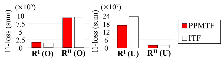
Figure 14: Reconstruction errors (sum of the $l_{1}$ loss) in $\mathbf{R}^{\mathrm{I}}$ and $\mathbf{R}^{\mathrm{II}}$ (TKY). “O” and “U” in the parentheses represent observed elements and unobserved elements, respectively.

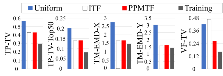
Figure 15: Utility of PPMTF and ITF (TKY).

Figure 14 shows the reconstruction errors in $\mathbf{R}^{\mathrm{I}}$ and $\mathbf{R}^{\mathrm{II}}$. PPMTF significantly outperforms ITF with regard to the reconstruction error of unobserved elements in $\mathbf{R}^{\mathrm{I}}$. This is because $\mathbf{R}^{\mathrm{I}}$ (which includes $47956\times 1000\times 1000$ elements) is much more sparse than $\mathbf{R}^{\mathrm{II}}$ (which includes $47956\times 1000\times 24$ elements) and $\mathbf{R}^{\mathrm{II}}$ compensates for the sparseness of $\mathbf{R}^{\mathrm{I}}$ in PPMTF by sharing $\mathbf{A}$ and $\mathbf{B}$. This is consistent with the experimental results in [66], where multiple tensor factorization works well especially when one of two tensors is extremely sparse.

Figure 15 shows the utility of PPMTF and ITF (here we do not run the PD test; even if we use the ($10,1$)-PD test, the utility of PPMTF is hardly changed, as shown in Figure 10). PPMTF significantly outperforms ITF in terms of VF-TV. We consider that this is because PPMTF trains $\mathbf{A}$ and $\mathbf{B}$, which model the similarity structure among users and locations, respectively, more accurately by sharing them between $\mathbf{R}^{\mathrm{I}}$ and $\mathbf{R}^{\mathrm{II}}$. Consequently, PPMTF generates user-specific (or cluster-specific) traces more effectively.

In summary, PPMTF addresses the sparseness of $\mathbf{R}^{\mathrm{I}}$ and achieves high utility by sharing factor matrices.

Appendix F Relationship between $k$ and the PD Test Pass Rate

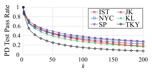
Figure 16: Relationship between $k$ and the PD test pass rate.

We evaluated the PD test pass rate, which is the proportion of synthetic traces that have passed the PD test to all synthetic traces when we changed $k$ from $1$ to $200$. We set the other parameters to the same values as in Section 4 (e.g., $\eta=1$, $|\mathcal{U}^{*}|=32000$).

Figure 16 shows the results obtained for six cities in FS. The PD test pass rate decreases with an increase in $k$. For example, the PD test pass rate is about $70\%$ when $k=10$, whereas it is about $20\%$ when $k=200$.

Note that when $k=200$, the PD test pass rate of IST ($17.9\%$) is lower than that of NYC ($26.9\%$), as shown in Figure 16. Nevertheless, PPMTF significantly outperforms Uniform with regard to all of the utility metrics in IST, as shown in Figure 10. This is because the number of users is very large in IST ($|\mathcal{U}|=219793$). Consequently, even if the PD test pass rate is low, many synthetic traces still pass the test and preserve various statistical features.

Therefore, PPMTF achieves high utility especially for a large-scale dataset.

Appendix G DP for the MTF parameters $\Theta$

Here we explain DP (Differential Privacy) [21, 22] as a privacy metric (Appendix G.1). Then we analyze the privacy budget $\varepsilon$ in DP for the MTF parameters $\Theta$ in PPMTF (Appendix G.2), and evaluate $\varepsilon$ for $\Theta$ using the Foursquare dataset (Appendix G.3).

G.1 Differential Privacy

We define the notion of neighboring data sets in the same way as [22, 43, 68] as follows. Let $\mathcal{S},\mathcal{S}^{\prime}\subseteq\mathcal{R}$ be two sets of training traces. We say $\mathcal{S}$ and $\mathcal{S}^{\prime}$ are neighboring if they differ by at most one trace and include the same number of traces, i.e., $|\mathcal{S}|=|\mathcal{S}^{\prime}|$. For example, given a trace $s^{\prime}_{1}\in\mathcal{R}$, $\mathcal{S}=\{s_{1},s_{2},s_{3}\}$ and $\mathcal{S}^{\prime}=\{s^{\prime}_{1},s_{2},s_{3}\}$ are neighboring. Then DP [21, 22] is defined as follows:

Definition 2 ($\varepsilon$-DP).

Let $\varepsilon\in\mathbb{R}_{\geq 0}$. A randomized algorithm $\mathcal{F}$ with domain $\mathcal{P}(\mathcal{R})$ provides $\varepsilon$-DP if for any neighboring $\mathcal{S},\mathcal{S}^{\prime}\subseteq\mathcal{R}$ and any $Z\subseteq\mathrm{Range}(\mathcal{F})$,

$$e^{-\varepsilon}p(\mathcal{F}(\mathcal{S}^{\prime})\in Z)\leq p(\mathcal{F}(\mathcal{S})\in Z)\leq e^{\varepsilon}p(\mathcal{F}(\mathcal{S}^{\prime})\in Z).$$ (8)

$\varepsilon$-DP guarantees that an adversary who has observed the output of $\mathcal{F}$ cannot determine, for any pair of $\mathcal{S}$ and $\mathcal{S}^{\prime}$, whether it comes from $\mathcal{S}$ or $\mathcal{S}^{\prime}$ (i.e., a particular user’s trace is included in the training trace set) with a certain degree of confidence. As the privacy budget $\varepsilon$ approaches $0$, $\mathcal{S}$ and $\mathcal{S}^{\prime}$ become almost equally likely, which means that a user’s privacy is strongly protected.

G.2 Theoretical Analysis

We now analyze the privacy budget $\varepsilon$ in DP for the MTF parameters $\Theta$ in PPMTF.

Let $\mathcal{F}_{\textit{PPMTF}}$ be our training algorithm in step (ii), which takes as input the training trace set $\mathcal{S}$ and outputs the MTF parameters $\Theta$. Assume that $\Theta$ is sampled from the exact posterior distribution $p(\Theta|\mathbf{R})$.

Recall that the maximum counts in $\mathbf{R}^{\mathrm{I}}$ and $\mathbf{R}^{\mathrm{II}}$ are $r_{max}^{\mathrm{I}}$ and $r_{max}^{\mathrm{II}}$, respectively, as defined in Section 3.2. Let $\kappa\in\mathbb{R}_{\geq 0}$ be a non-negative real number such that $\hat{r}_{n,i,j}^{\mathrm{I}}\in[-\kappa,\allowbreak r_{max}^{\mathrm{I}}+\kappa]$ and $\hat{r}_{n,i,j}^{\mathrm{II}}\in[-\kappa,r_{max}^{\mathrm{II}}+\kappa]$ for each triple ($n,i,j$). The value of $\kappa$ can be made small by iterating the sampling of $\Theta$ until we find $\Theta$ with small $\kappa$ [43]. Note that this “retry if fail” procedure guarantees that $\Theta$ is sampled from the posterior distribution under the constraint that $\hat{r}_{n,i,j}^{\mathrm{I}}$ and $\hat{r}_{n,i,j}^{\mathrm{II}}$ are bounded as above (see the proof of Theorem 1 in [43]). Then we obtain:

Proposition 1.

$\mathcal{F}_{\textit{PPMTF}}$ provides $\varepsilon$-DP, where

$$\varepsilon= \alpha\left(\min\{3\lambda^{\mathrm{I}},\lambda^{\mathrm{I}}+\rho^{\mathrm{I}}\}(r_{max}^{\mathrm{I}}+\kappa)^{2}\right.$$

$$\left.+\min\{3\lambda^{\mathrm{II}},\lambda^{\mathrm{II}}+\rho^{\mathrm{II}}\}(r_{max}^{\mathrm{II}}+\kappa)^{2}\right).$$ (9)

Proof.

By (3), $\ln p(\Theta|\mathbf{R})$ can be written as follows:

$$\ln p(\Theta|\mathbf{R})$$

$$= \ln p(\mathbf{R}|\Theta)+\ln p(\Theta)-\ln p(\mathbf{R})~{}~{}~{}(\text{by Bayes' theorem})$$

$$= -\sum_{n=1}^{|\mathcal{U}|}\sum_{i=1}^{|\mathcal{X}|}\sum_{j=1}^{|\mathcal{X}|}I_{n,i,j}^{\mathrm{I}}\left(\frac{\alpha(r_{n,i,j}^{\mathrm{I}}-\hat{r}_{n,i,j}^{\mathrm{I}})^{2}}{2}+\ln\sqrt{\frac{\alpha}{2\pi}}\right)$$

$$-\sum_{n=1}^{|\mathcal{U}|}\sum_{i=1}^{|\mathcal{X}|}\sum_{j=1}^{|\mathcal{L}|}I_{n,i,j}^{\mathrm{II}}\left(\frac{\alpha(r_{n,i,j}^{\mathrm{II}}-\hat{r}_{n,i,j}^{\mathrm{II}})^{2}}{2}+\ln\sqrt{\frac{\alpha}{2\pi}}\right)$$

$$+\ln p(\Theta)-\ln p(\mathbf{R}).$$ (10)

The sum of the first and second terms in (10) is the log-likelihood $\ln p(\mathbf{R}|\Theta)$, and is bounded by the trimming that ensures $r_{n,i,j}^{\mathrm{I}}\in[0,r_{max}^{\mathrm{I}}]$ and $r_{n,i,j}^{\mathrm{II}}\in[0,r_{max}^{\mathrm{II}}]$.

Let $G$ be a function that takes as input $\mathbf{R}$ and $\Theta$ and outputs $G(\mathbf{R},\Theta)\in\mathbb{R}$ as follows:

$$G(\mathbf{R},\Theta)= \sum_{n=1}^{|\mathcal{U}|}\sum_{i=1}^{|\mathcal{X}|}\sum_{j=1}^{|\mathcal{X}|}\frac{\alpha\hskip 1.42262ptI_{n,i,j}^{\mathrm{I}}(r_{n,i,j}^{\mathrm{I}}-\hat{r}_{n,i,j}^{\mathrm{I}})^{2}}{2}$$

$$+\sum_{n=1}^{|\mathcal{U}|}\sum_{i=1}^{|\mathcal{X}|}\sum_{j=1}^{|\mathcal{L}|}\frac{\alpha\hskip 1.42262ptI_{n,i,j}^{\mathrm{II}}(r_{n,i,j}^{\mathrm{II}}-\hat{r}_{n,i,j}^{\mathrm{II}})^{2}}{2}$$

$$-\ln p(\Theta).$$ (11)

Note that $\ln\sqrt{\frac{\alpha}{2\pi}}$ and $\ln p(\mathbf{R})$ in (10) do not depend on $\Theta$. Thus, by (11), $\ln p(\Theta|\mathbf{R})$ in (10) can be expressed as:

$$p(\Theta|\mathbf{R})=\frac{\exp[-G(\mathbf{R},\Theta)]}{\int_{\Theta}\exp[-G(\mathbf{R},\Theta)]d\Theta}.$$ (12)

Then, Proposition 1 can be proven by using the fact that $\mathcal{F}_{PPMTF}$ is the exponential mechanism [22] that uses $-G(\mathbf{R},\Theta)$ as a utility function. Specifically, let $\mathbf{R}^{\prime}$ be the tuple of two tensors that differ from $\mathbf{R}$ at most one user’s elements; i.e., $\mathbf{R}$ and $\mathbf{R}^{\prime}$ are neighboring. We write $\mathbf{R}\sim\mathbf{R}^{\prime}$ to represent that $\mathbf{R}$ and $\mathbf{R}^{\prime}$ are neighboring. Let $\Delta G\in\mathbb{R}$ be the sensitivity of $G$ given by:

$$\Delta G=\underset{\Theta}{\max}\underset{\mathbf{R},\mathbf{R}^{\prime}:\mathbf{R}\sim\mathbf{R}^{\prime}}{\max}|G(\mathbf{R},\Theta)-G(\mathbf{R}^{\prime},\Theta)|.$$ (13)

Here we note that when $\rho^{\mathrm{I}}$ is large, many zero elements are common in $\mathbf{R}^{\mathrm{I}}$ and ${\mathbf{R}^{\prime}}^{\mathrm{I}}$. Specifically, for each user, we can randomly select $\rho^{\mathrm{I}}$ zero elements as follows: (i) randomly select $\rho^{\mathrm{I}}$ elements from $\mathbf{R}^{\mathrm{I}}$ (including non-zero elements), (ii) count the number $\rho_{0}^{\mathrm{I}}$ ($\leq\lambda^{\mathrm{I}}$) of non-zero elements in the selected elements, (iii) randomly reselect $\rho_{0}^{\mathrm{I}}$ elements from zero (and not selected) elements in $\mathbf{R}^{\mathrm{I}}$. Note that this algorithm eventually selects $\rho^{\mathrm{I}}$ zero elements from $\mathbf{R}^{\mathrm{I}}$ at random. In this case, for each user, at least $\max\{\rho^{\mathrm{I}}-2\lambda^{\mathrm{I}},0\}$ zero elements are common in $\mathbf{R}^{\mathrm{I}}$ and ${\mathbf{R}^{\prime}}^{\mathrm{I}}$ (since $\mathbf{R}^{\mathrm{I}}$ and ${\mathbf{R}^{\prime}}^{\mathrm{I}}$ have at most $2\lambda^{\mathrm{I}}$ reselected elements in total).

Except for such common zero elements, $I_{n,i,j}^{\mathrm{I}}$ in (11) takes 1 at most $\min\{3\lambda^{\mathrm{I}},\lambda^{\mathrm{I}}+\rho^{\mathrm{I}}\}$ elements for each user (since $(\lambda^{\mathrm{I}}+\rho^{\mathrm{I}})-(\rho^{\mathrm{I}}-2\lambda^{\mathrm{I}})=3\lambda^{\mathrm{I}}$). Similarly, except for common zero elements, $I_{n,i,j}^{\mathrm{II}}$ in (11) takes 1 at most $\min\{3\lambda^{\mathrm{II}},\lambda^{\mathrm{II}}+\rho^{\mathrm{II}}\}$ elements for each user. In addition, $r_{n,i,j}^{\mathrm{I}}\in[0,r_{max}^{\mathrm{I}}]$, $r_{n,i,j}^{\mathrm{II}}\in[0,r_{max}^{\mathrm{II}}]$, $\hat{r}_{n,i,j}^{\mathrm{I}}\in[-\kappa,r_{max}^{\mathrm{I}}+\kappa]$, and $\hat{r}_{n,i,j}^{\mathrm{II}}\in[-\kappa,r_{max}^{\mathrm{II}}+\kappa]$ for each triple ($n,i,j$), as described in Section 3.5. Moreover, the “retry if fail” procedure, which iterates the sampling of $\Theta$ until $\hat{r}_{n,i,j}^{\mathrm{I}}$ and $\hat{r}_{n,i,j}^{\mathrm{II}}$ are bounded as above, guarantees that $\Theta$ is sampled from the posterior distribution under this constraint [43].

Consequently, the sum of the first and second terms in (11) is less than (resp. more than) or equal to $\frac{\varepsilon}{2}$ (resp. $0$), where $\varepsilon$ is given by (9). Then, since the third term in (11) is the same for $G(\mathbf{R},\Theta)$ and $G(\mathbf{R}^{\prime},\Theta)$ in (13), $\Delta G$ can be bounded above by $\frac{\varepsilon}{2}$: i.e., $\Delta G\leq\frac{\varepsilon}{2}$. Since the exponential mechanism with sensitivity $\frac{\varepsilon}{2}$ provides $\varepsilon$-DP [22], $\mathcal{F}_{PPMTF}$ provides $\varepsilon$-DP. ∎

$\varepsilon$ for a single location.  We also analyze $\varepsilon$ for neighboring data sets $\mathbf{R}$ and $\mathbf{R}^{\prime}$ that differ in a single location. Here we assume $\rho^{\mathrm{I}}=\rho^{\mathrm{II}}=0$ to simplify the analysis (if $\rho^{\mathrm{I}}>0$ or $\rho^{\mathrm{II}}>0$, then $\varepsilon$ will be larger because selected zero elements can be different in $\mathbf{R}$ and $\mathbf{R}^{\prime}$). In this case, $\mathbf{R}^{\mathrm{I}}$ and ${\mathbf{R}^{\prime}}^{\mathrm{I}}$ (resp. $\mathbf{R}^{\mathrm{II}}$ and ${\mathbf{R}^{\prime}}^{\mathrm{II}}$) differ in at most two (resp. four) elements, and the value in each element differs by $1$. Then by (11) and (13), we obtain:

$$\Delta G \leq 2\cdot\frac{\alpha}{2}\left((r_{max}^{\mathrm{I}}+\kappa)^{2}-(r_{max}^{\mathrm{I}}+\kappa-1)^{2}\right)$$

$$\hskip 9.95845pt+4\cdot\frac{\alpha}{2}\left((r_{max}^{\mathrm{II}}+\kappa)^{2}-(r_{max}^{\mathrm{II}}+\kappa-1)^{2})\right)$$

$$=\alpha(2r_{max}^{\mathrm{I}}+4r_{max}^{\mathrm{II}}+6\kappa-3),$$

and therefore $\varepsilon=\alpha(4r_{max}^{\mathrm{I}}+8r_{max}^{\mathrm{II}}+12\kappa-6)$.

Note that a trace $y$ is synthesized from $\Theta$ after $\mathcal{F}_{\textit{PPMTF}}$ outputs $\Theta$. Then by the immunity to post-processing [22], $\mathcal{F}_{\textit{PPMTF}}$ also provides $\varepsilon$-DP for all synthetic traces. However, $\varepsilon$ needs to be large to achieve high utility, as shown in Appendix G.3.

G.3 Experimental Evaluation

We evaluated the privacy budget $\varepsilon$ in DP for $\Theta$ and the utility by changing $\alpha$ in Proposition 1 from $10^{-6}$ and $10^{3}$ using the Foursquare dataset [69]. Figure 17 shows the results in IST (Istanbul), where $\varepsilon$ is the value in Proposition 1 when $\kappa=0$. In practice, $\varepsilon$ can be larger than this value because $\kappa\geq 0$.

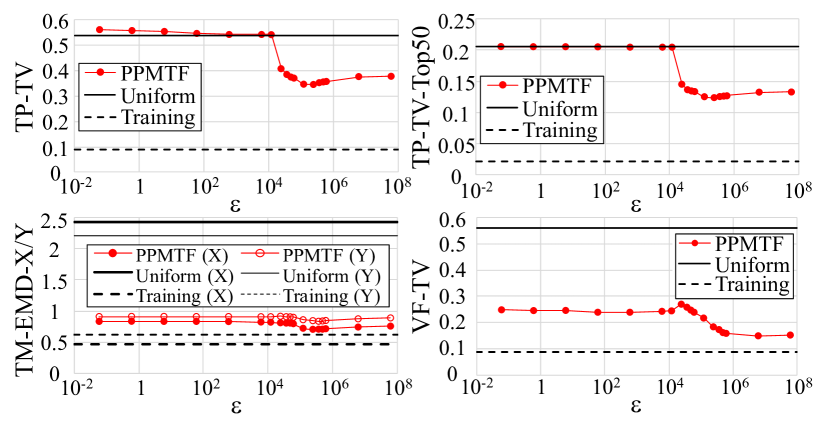
Figure 17: Relation between $\varepsilon$ and utility in IST ($\kappa=0$).

Figure 17 shows that $\varepsilon$ needs to be larger than $2\times 10^{4}$ to provide high utility. This is because $\alpha$ in Proposition 1 needs to be large to achieve high utility. Specifically, by (3), $\alpha$ needs to be large so that $\hat{r}_{n,i,j}^{\mathrm{I}}$ and $\hat{r}_{n,i,j}^{\mathrm{II}}$ in (3) are close to $r_{n,i,j}^{\mathrm{I}}$ and $r_{n,i,j}^{\mathrm{II}}$, respectively. For example, when $\alpha=0.01$ (i.e., standard deviation in (3) $=10$), transition/visit-counts can be frequently changed by $\pm{10}$ after sampling (e.g., $\hat{r}_{n,i,j}^{\mathrm{I}}=r_{n,i,j}^{\mathrm{I}}\pm 10$), which destroys the utility. In Figure 17, we need $\alpha\geq 0.4$ to achieve high utility, which results in $\varepsilon>2\times 10^{4}$.

If we consider neighboring data sets $\mathcal{S}$ and $\mathcal{S}^{\prime}$ that differ in a single location (rather than one trace), $\varepsilon$ becomes much smaller. However, $\varepsilon$ is still large. Specifically, if $\kappa=\rho^{\mathrm{I}}=\rho^{\mathrm{II}}=0$, then $\varepsilon=\alpha(4r_{max}^{\mathrm{I}}+8r_{max}^{\mathrm{II}}-6)$; otherwise, $\varepsilon$ is larger than this value (see Appendix G.2). Thus, when $\alpha=0.4$, the privacy budget is $\varepsilon=45.6$ or more (since $r_{max}^{\mathrm{I}}=r_{max}^{\mathrm{II}}=10$).

Finally, we note that adding the Laplacian noise to $\Theta$ (rather than sampling $\Theta$) does not provide DP. For example, assume that $\Theta$ is trained from $\mathcal{S}$ by the MAP (Maximum a Posteriori) estimation algorithm $\mathcal{F}$ [10], which calculates $\Theta$ that maximizes $p(\Theta|\mathcal{S})$; i.e., $\mathcal{F}(\mathcal{S})=\operatornamewithlimits{argmax}_{\Theta}p(\Theta|\mathcal{S})$. If $p(\Theta|\mathcal{S})$ is uniform (or nearly uniform), then $\mathcal{F}(\mathcal{S}^{\prime})$ can take any value for neighboring trace set $\mathcal{S}^{\prime}$. Therefore, the sensitivity is unbounded and adding the Laplacian noise does not provide DP.

For these reasons, providing a small $\varepsilon$ in DP is difficult in our location synthesizer.

Appendix H Details of Gibbs Sampling

Let $\Psi=(\Psi_{\mathbf{A}},\Psi_{\mathbf{B}},\Psi_{\mathbf{C}},\Psi_{\mathbf{D}})$. $\Psi_{\mathbf{A}}$, $\Psi_{\mathbf{B}}$, $\Psi_{\mathbf{C}}$, and $\Psi_{\mathbf{D}}$ are called hyper-parameters in Bayesian statistics. We explain details of how to sample the hyper-parameters $\Psi$ and the MTF parameters $\Theta$ using Gibbs sampling.

In the $t$-th iteration, we sample $\Psi_{\mathbf{A}}^{(t)}$, $\Psi_{\mathbf{B}}^{(t)}$, $\Psi_{\mathbf{C}}^{(t)}$, $\Psi_{\mathbf{D}}^{(t)}$, $\mathbf{A}^{(t)}$, $\mathbf{B}^{(t)}$, $\mathbf{C}^{(t)}$, and $\mathbf{D}^{(t)}$ from the conditional distribution given the current values of the other variables. Specifically, based on the graphical model in Figure 4, we sample each variable as follows:

$$\Psi_{\mathbf{A}}^{(t)} \sim p(\Psi_{\mathbf{A}}|\mathbf{A}^{(t-1)})$$ (14)

$$\Psi_{\mathbf{B}}^{(t)} \sim p(\Psi_{\mathbf{B}}|\mathbf{B}^{(t-1)})$$ (15)

$$\Psi_{\mathbf{C}}^{(t)} \sim p(\Psi_{\mathbf{C}}|\mathbf{C}^{(t-1)})$$ (16)

$$\Psi_{\mathbf{D}}^{(t)} \sim p(\Psi_{\mathbf{D}}|\mathbf{D}^{(t-1)})$$ (17)

$$\mathbf{A}^{(t)} \sim p(\mathbf{A}|\mathbf{R},\mathbf{B}^{(t-1)},\mathbf{C}^{(t-1)},\mathbf{D}^{(t-1)},\Psi_{\mathbf{A}}^{(t)})$$ (18)

$$\mathbf{B}^{(t)} \sim p(\mathbf{B}|\mathbf{R},\mathbf{A}^{(t)},\mathbf{C}^{(t-1)},\mathbf{D}^{(t-1)},\Psi_{\mathbf{B}}^{(t)})$$ (19)

$$\mathbf{C}^{(t)} \sim p(\mathbf{C}|\mathbf{R}^{\mathrm{I}},\mathbf{A}^{(t)},\mathbf{B}^{(t)},\Psi_{\mathbf{C}}^{(t)})$$ (20)

$$\mathbf{D}^{(t)} \sim p(\mathbf{D}|\mathbf{R}^{\mathrm{II}},\mathbf{A}^{(t)},\mathbf{B}^{(t)},\Psi_{\mathbf{D}}^{(t)})$$ (21)

Below we explain details of how to compute the sampling distribution for the hyper-parameters and MTF parameters.

Sampling of the hyper-parameters.  We explain the computation of the right-hand side of (14) in Gibbs sampling. We omit the computation of (15), (16), and (17) because they are computed in the same way as (14); i.e., (15), (16), and (17) can be computed by replacing $\mathbf{A}$ in (14) with $\mathbf{B}$, $\mathbf{C}$, and $\mathbf{D}$, respectively. Below we omit superscripts $(t)$ and $(t-1)$.

$p(\Psi_{\mathbf{A}}|\mathbf{A})$ in (14) can be computed by using the fact that the Normal-Wishart distribution is a conjugate prior of the multivariate normal distribution [10]. Specifically, following [59], we compute $p(\Psi_{\mathbf{A}}|\mathbf{A})$ in (14) as follows:

$$p(\Psi_{\mathbf{A}}|\mathbf{A}) ={\textstyle\frac{p(\mathbf{A}|\Psi_{\mathbf{A}})p(\Psi_{\mathbf{A}})}{p(\mathbf{A})}}~{}~{}\text{(by Bayes' theorem)}$$

$$=\mathcal{N}(\mu_{\mathbf{A}}|\mu_{0}^{*},(\beta_{0}^{*}\Lambda_{\mathbf{A}})^{\!-1})\mathcal{W}(\Lambda_{\mathbf{A}}|W_{0}^{*},\nu_{0}^{*}),$$ (22)

where

$$\mu_{0}^{*} ={\textstyle\frac{\beta_{0}\mu_{0}+|\mathcal{U}|\bar{\mathbf{a}}}{\beta_{0}+|\mathcal{U}|}}$$ (23)

$$\beta_{0}^{*} =\beta_{0}+|\mathcal{U}|$$ (24)

$$W_{0}^{*} =\left[W_{0}^{\!-1}+|\mathcal{U}|\bar{\mathbf{S}}+{\textstyle\frac{\beta_{0}|\mathcal{U}|}{\beta_{0}+|\mathcal{U}|}}(\mu_{0}-\bar{\mathbf{a}})^{\top}(\mu_{0}-\bar{\mathbf{a}})\right]^{\!-1}$$ (25)

$$\nu_{0}^{*} =\nu_{0}+|\mathcal{U}|$$ (26)

$$\bar{\mathbf{a}} ={\textstyle\frac{1}{|\mathcal{U}|}}\sum_{n=1}^{|\mathcal{U}|}\mathbf{a}_{n}$$ (27)

$$\bar{\mathbf{S}} ={\textstyle\frac{1}{|\mathcal{U}|}}\sum_{n=1}^{|\mathcal{U}|}\mathbf{a}_{n}^{\top}\mathbf{a}_{n}.$$ (28)

Therefore, we compute $p(\Psi_{\mathbf{A}}|\mathbf{A})$ by (22) to (28). Then we sample $\Psi_{\mathbf{A}}$ from $p(\Psi_{\mathbf{A}}|\mathbf{A})$.

Sampling of the MTF parameters.  Next we explain the computation of (18) and (20). We omit the computation of (19) and (21) because they are computed in the same way as (18) and (20), respectively; i.e., (19) and (21) can be computed by exchanging $\mathbf{A}$ for $\mathbf{B}$ in (18), and $\mathbf{C}$ for $\mathbf{D}$ in (20).

$p(\mathbf{A}|\mathbf{R},\mathbf{B},\mathbf{C},\mathbf{D},\Psi_{\mathbf{A}})$ in (18) can be written as follows:

$$p(\mathbf{A}|\mathbf{R},\mathbf{B},\mathbf{C},\mathbf{D},\Psi_{\mathbf{A}}) =\prod_{n=1}^{|\mathcal{U}|}p(\mathbf{a}_{n}|\mathbf{R}_{n}^{\mathrm{I}},\mathbf{R}_{n}^{\mathrm{II}},\mathbf{B},\mathbf{C},\mathbf{D},\Psi_{\mathbf{A}}),$$ (29)

where $\mathbf{R}_{n}^{\mathrm{I}}$ and $\mathbf{R}_{n}^{\mathrm{II}}$ are the $n$-th matrices in $\mathbf{R}^{\mathrm{I}}$ and $\mathbf{R}^{\mathrm{II}}$, respectively. By Bayes’ theorem and the graphical model in Figure 4, $p(\mathbf{a}_{n}|\mathbf{R}_{n}^{\mathrm{I}},\mathbf{R}_{n}^{\mathrm{II}},\mathbf{B},\mathbf{C},\mathbf{D},\Psi_{\mathbf{A}})$ in (29) can be written as follows:

$$p(\mathbf{a}_{n}|\mathbf{R}_{n}^{\mathrm{I}},\mathbf{R}_{n}^{\mathrm{II}},\mathbf{B},\mathbf{C},\mathbf{D},\Psi_{\mathbf{A}})$$

$$= \frac{p(\mathbf{R}_{n}^{\mathrm{I}},\mathbf{R}_{n}^{\mathrm{II}}|\mathbf{a}_{n},\mathbf{B},\mathbf{C},\mathbf{D},\Psi_{\mathbf{A}})p(\mathbf{a}_{n}|\mathbf{B},\mathbf{C},\mathbf{D},\Psi_{\mathbf{A}})}{p(\mathbf{R}_{n}^{\mathrm{I}},\mathbf{R}_{n}^{\mathrm{II}}|\mathbf{B},\mathbf{C},\mathbf{D},\Psi_{\mathbf{A}})}$$

$$= \frac{p(\mathbf{R}_{n}^{\mathrm{I}}|\mathbf{a}_{n},\mathbf{B},\mathbf{C})p(\mathbf{R}_{n}^{\mathrm{II}}|\mathbf{a}_{n},\mathbf{B},\mathbf{D})p(\mathbf{a}_{n}|\Psi_{\mathbf{A}})}{p(\mathbf{R}_{n}^{\mathrm{I}},\mathbf{R}_{n}^{\mathrm{II}}|\mathbf{B},\mathbf{C},\mathbf{D},\Psi_{\mathbf{A}})}.$$ (30)

Note that $p(\mathbf{R}_{n}^{\mathrm{I}}|\mathbf{a}_{n},\mathbf{B},\mathbf{C})$, $p(\mathbf{R}_{n}^{\mathrm{II}}|\mathbf{a}_{n},\mathbf{B},\mathbf{D})$, and $p(\mathbf{a}_{n}|\Psi_{\mathbf{A}})$ are normal distributions (as described in Section 3.3), and $p(\mathbf{R}_{n}^{\mathrm{I}},\mathbf{R}_{n}^{\mathrm{II}}|\mathbf{B},\mathbf{C},\mathbf{D},\Psi_{\mathbf{A}})$ is a normalization constant so that the sum of $p(\mathbf{a}_{n}|\mathbf{R}_{n}^{\mathrm{I}},\mathbf{R}_{n}^{\mathrm{II}},\mathbf{B},\mathbf{C},\mathbf{D},\Psi_{\mathbf{A}})$ over all values of $\mathbf{a}_{n}$ is one. In addition, let $\mathbf{bc}_{ij}\in\mathbb{R}^{z}$ and $\mathbf{bd}_{ij}\in\mathbb{R}^{z}$ are shorthand for $\mathbf{b}_{i}\circ\mathbf{c}_{j}$ and $\mathbf{b}_{i}\circ\mathbf{d}_{j}$, respectively, where $\circ$ represents the Hadamard product. Then by (2), $\hat{r}_{n,i,j}^{\mathrm{I}}$ and $\hat{r}_{n,i,j}^{\mathrm{II}}$ can be expressed as: $\hat{r}_{n,i,j}^{\mathrm{I}}=\mathbf{a}_{n}^{\top}\mathbf{bc}_{ij}$ and $\hat{r}_{n,i,j}^{\mathrm{II}}=\mathbf{a}_{n}^{\top}\mathbf{bd}_{ij}$, respectively.

Thus, $p(\mathbf{a}_{n}|\mathbf{R}_{n}^{\mathrm{I}},\mathbf{R}_{n}^{\mathrm{II}},\mathbf{B},\mathbf{C},\mathbf{D},\Psi_{\mathbf{A}})$ can be expressed as:

$$p(\mathbf{a}_{n}|\mathbf{R}_{n}^{\mathrm{I}},\mathbf{R}_{n}^{\mathrm{II}},\mathbf{B},\mathbf{C},\mathbf{D},\Psi_{\mathbf{A}})$$

$$= d_{1}\exp\Biggl{[}\sum_{i=1}^{|\mathcal{X}|}\sum_{j=1}^{|\mathcal{X}|}\alpha\hskip 0.56905ptI_{n,i,j}^{\mathrm{I}}(\mathbf{a}_{n}^{\top}\mathbf{bc}_{ij}-r_{n,i,j}^{\mathrm{I}})^{2}$$

$$\hskip 39.83385pt+\sum_{i=1}^{|\mathcal{X}|}\sum_{j=1}^{|\mathcal{L}|}\alpha\hskip 0.56905ptI_{n,i,j}^{\mathrm{II}}(\mathbf{a}_{n}^{\top}\mathbf{bd}_{ij}-r_{n,i,j}^{\mathrm{II}})^{2}$$

$$\hskip 39.83385pt+(\mathbf{a}_{n}-\mu_{A})^{\top}\Lambda_{\mathbf{A}}(\mathbf{a}_{n}-\mu_{A})\Biggr{]},$$ (31)

where $d_{1}\in\mathbb{R}$ is a normalization constant.

To simplify (29) and (31), we use the following two facts. First, for any $v\in\mathbb{R}$ and any $\mathbf{w}\in\mathbb{R}^{z}$, we obtain:

$$v^{2} =v(\mathbf{w}^{-1\top}\mathbf{w})(\mathbf{w}^{\top}\mathbf{w}^{-1})v$$

$$=((v\mathbf{w}^{-1})^{\top}\mathbf{w})(\mathbf{w}^{\top}(v\mathbf{w}^{-1}))$$

$$=(v\mathbf{w}^{-1})^{\top}(\mathbf{w}\mathbf{w}^{\top})(v\mathbf{w}^{-1}))~{}~{}\text{(by associativity)}.$$

Thus,

$$(\mathbf{a}_{n}^{\top}\mathbf{bc}_{ij}-r_{n,i,j}^{\mathrm{I}})^{2}$$

$$= (\mathbf{a}_{n}-r_{n,i,j}^{\mathrm{I}}\mathbf{bc}_{ij}^{-1})^{\top}(\mathbf{bc}_{ij}\mathbf{bc}_{ij}^{\top})(\mathbf{a}_{n}-r_{n,i,j}^{\mathrm{I}}\mathbf{bc}_{ij}^{-1})$$

and

$$(\mathbf{a}_{n}^{\top}\mathbf{bd}_{ij}-r_{n,i,j}^{\mathrm{II}})^{2}$$

$$= (\mathbf{a}_{n}-r_{n,i,j}^{\mathrm{II}}\mathbf{bd}_{ij}^{-1})^{\top}(\mathbf{bd}_{ij}\mathbf{bd}_{ij}^{\top})(\mathbf{a}_{n}-r_{n,i,j}^{\mathrm{II}}\mathbf{bd}_{ij}^{-1}).$$

Therefore, we obtain:

$$p(\mathbf{a}_{n}|\mathbf{R}_{n}^{\mathrm{I}},\mathbf{R}_{n}^{\mathrm{II}},\mathbf{B},\mathbf{C},\mathbf{D},\Psi_{\mathbf{A}})$$

$$= d_{2}\prod_{i=1}^{|\mathcal{X}|}\prod_{j=1}^{|\mathcal{X}|}\mathcal{N}(\mathbf{a}_{n}|r_{n,i,j}^{\mathrm{I}}\mathbf{bc}_{ij}^{-1},(\alpha\hskip 0.56905ptI_{n,i,j}^{\mathrm{I}}\mathbf{bc}_{ij}\mathbf{bc}_{ij}^{\top})^{-1})$$

$$\hskip 11.38109pt\cdot\prod_{i=1}^{|\mathcal{X}|}\prod_{j=1}^{|\mathcal{L}|}\mathcal{N}(\mathbf{a}_{n}|r_{n,i,j}^{\mathrm{II}}\mathbf{bd}_{ij}^{-1},(\alpha\hskip 0.56905ptI_{n,i,j}^{\mathrm{II}}\mathbf{bd}_{ij}\mathbf{bd}_{ij}^{\top})^{-1})$$

$$\hskip 11.38109pt\cdot\mathcal{N}(\mathbf{a}_{n}|\mu_{A},\Lambda_{\mathbf{A}}^{-1}),$$ (32)

where $d_{2}\in\mathbb{R}$ is a normalization constant.

Second, the product of two Gaussian densities is proportional to a Gaussian density [55]. Specifically, for any $\mathbf{w}\in\mathbb{R}^{z}$, any $\mathbf{m}_{1},\mathbf{m}_{2}\in\mathbb{R}^{z}$, and any $\Lambda_{1},\Lambda_{2}\in\mathbb{R}^{z\times z}$, we obtain:

$$\mathcal{N}(\mathbf{w}|\mathbf{m}_{1},\Lambda_{1}^{-1})\cdot\mathcal{N}(\mathbf{w}|\mathbf{m}_{2},\Lambda_{2}^{-1})=d_{3}\mathcal{N}(\mathbf{w}|\mathbf{m}_{c},\Lambda_{c}^{-1}),$$ (33)

where

$$d_{3} =\mathcal{N}(\mathbf{m}_{1}|\mathbf{m}_{2},\Lambda_{1}^{-1}+\Lambda_{2}^{-1})$$

$$\mathbf{m}_{c} =(\Lambda_{1}+\Lambda_{2})^{-1}(\Lambda_{1}\mathbf{m}_{1}+\Lambda_{2}\mathbf{m}_{2})$$

$$\Lambda_{c} =\Lambda_{1}+\Lambda_{2}.$$ (34)

By (32), (33), and (34), $p(\mathbf{A}|\mathbf{R},\mathbf{B},\mathbf{C},\mathbf{D},\Psi_{\mathbf{A}})$ in (29) can be written as follows:

$$p(\mathbf{A}|\mathbf{R},\mathbf{B},\mathbf{C},\mathbf{D},\Psi_{\mathbf{A}})=\prod_{n=1}^{|\mathcal{U}|}\mathcal{N}(\mathbf{a}_{n}|\mu_{\mathbf{A},n}^{*},\Lambda_{\mathbf{A},n}^{*}),$$ (35)

where

$$\Lambda_{\mathbf{A},n}^{*} =\Lambda_{\mathbf{A}}+\alpha\hskip 0.56905ptI_{n,i,j}^{\mathrm{I}}\sum_{i=1}^{|\mathcal{X}|}\sum_{j=1}^{|\mathcal{X}|}(\mathbf{bc}_{ij}\mathbf{bc}_{ij}^{\top})$$ (36)

$$\hskip 9.95845pt+\alpha\hskip 0.56905ptI_{n,i,j}^{\mathrm{II}}\sum_{i=1}^{|\mathcal{X}|}\sum_{j=1}^{|\mathcal{L}|}(\mathbf{bd}_{ij}\mathbf{bd}_{ij}^{\top})$$

$$\mu_{\mathbf{A},n}^{*} =[\Lambda_{\mathbf{A},n}^{*}]^{-1}\left(\Lambda_{\mathbf{A}}\mu_{\mathbf{A}}+\alpha I_{n,i,j}^{\mathrm{I}}\sum_{i=1}^{|\mathcal{X}|}\sum_{j=1}^{|\mathcal{X}|}r_{n,i,j}^{\mathrm{I}}\mathbf{bc}_{ij}\right.$$

$$\hskip 54.06023pt+\left.\alpha I_{n,i,j}^{\mathrm{II}}\sum_{i=1}^{|\mathcal{X}|}\sum_{j=1}^{|\mathcal{L}|}r_{n,i,j}^{\mathrm{II}}\mathbf{bd}_{ij}\right).$$ (37)

Similarly, $p(\mathbf{C}|\mathbf{R}^{\mathrm{I}},\mathbf{A},\mathbf{B},\Psi_{\mathbf{C}})$ in (20) can be written as follows:

$$p(\mathbf{C}|\mathbf{R}^{\mathrm{I}},\mathbf{A},\mathbf{B},\Psi_{\mathbf{C}}) =\prod_{j=1}^{|\mathcal{X}|}p(\mathbf{c}_{j}|\mathbf{R}^{\mathrm{I}},\mathbf{A},\mathbf{B},\Psi_{\mathbf{C}})$$

$$=\prod_{j=1}^{|\mathcal{X}|}\mathcal{N}(\mathbf{c}_{j}|\mu_{\mathbf{C},j}^{*},\Lambda_{\mathbf{C},j}^{*}),$$ (38)

where

$$\Lambda_{\mathbf{C},j}^{*} =\Lambda_{\mathbf{C}}+\alpha\hskip 0.56905ptI_{n,i,j}^{\mathrm{I}}\sum_{n=1}^{|\mathcal{U}|}\sum_{i=1}^{|\mathcal{X}|}\mathbf{ab}_{ni}\mathbf{ab}_{ni}^{\top}$$ (39)

$$\mu_{\mathbf{C},j}^{*} =[\Lambda_{\mathbf{C},j}^{*}]^{-1}\left(\Lambda_{\mathbf{C}}\mu_{\mathbf{C}}+\alpha\hskip 0.56905ptI_{n,i,j}^{\mathrm{I}}\sum_{n=1}^{|\mathcal{U}|}\sum_{i=1}^{|\mathcal{X}|}r_{n,i,j}^{\mathrm{I}}\mathbf{ab}_{ni}\right)$$ (40)

and $\mathbf{ab}_{ni}$ is shorthand for $\mathbf{a}_{n}\circ\mathbf{b}_{i}$. Thus we compute $p(\mathbf{A}|\mathbf{R},\allowbreak\mathbf{B},\mathbf{C},\mathbf{D},\Psi_{\mathbf{A}})$ and $p(\mathbf{C}|\mathbf{R}^{\mathrm{I}},\mathbf{A},\mathbf{B},\allowbreak\Psi_{\mathbf{C}})$ by (35) to (37) and (38) to (40), respectively. Then we sample $\mathbf{A}$ and $\mathbf{C}$ from these distributions.

References

- [1] Tool: Privacy-preserving multiple tensor factorization (PPMTF). https://github.com/PPMTF/PPMTF.
- [2] PWS Cup 2019. https://www.iwsec.org/pws/2019/cup19_e.html, 2019.
- [3] C. C. Aggarwal. Recommender Systems. Springer, 2016.
- [4] R. Albright, J. Cox, D. Duling, A. N. Langville, and C. D. Meyer. Algorithms, initializations, and convergence for the nonnegative matrix factorization. SAS Technical Report, pages 1–18, 2014.
- [5] J. Biagioni and J. Eriksson. Inferring road maps from global positioning system traces: Survey and comparative evaluation. Journal of the Transportation Research Board, 2291(2291):61–71, 2012.
- [6] I. Bilogrevic, K. Huguenin, M. Jadliwala, F. Lopez, J.-P. Hubaux, P. Ginzboorg, and V. Niemi. Inferring social ties in academic networks using short-range wireless communications. In Proceedings of the 12th ACM Workshop on Privacy in the Electronic Society (WPES’13), pages 179–188, 2013.
- [7] V. Bindschaedler and R. Shokri. Synthetic location traces generator (sglt). https://vbinds.ch/node/70.
- [8] V. Bindschaedler and R. Shokri. Synthesizing plausible privacy-preserving location traces. In Proceedings of the 2016 IEEE Symposium on Security and Privacy (S&P’16), pages 546–563, 2016.
- [9] V. Bindschaedler, R. Shokri, and C. A. Gunter. Plausible deniability for privacy-preserving data synthesis. Proceedings of the VLDB Endowment, 10(5):481–492, 2017.
- [10] C. Bishop. Pattern Recognition and Machine Learning. Springer, 2006.
- [11] K. Chatzikokolakis, E. Elsalamouny, C. Palamidessi, and A. Pazii. Methods for location privacy: A comparative overview. Foundations and Trends in Privacy and Security, 1(4):199–257, 2017.
- [12] R. Chen, G. Acs, and C. Castelluccia. Differentially private sequential data publication via variable-length n-grams. In Proceedings of the 19th ACM Conference on Computer and Communications Security (CCS’12), pages 638–649, 2012.
- [13] R. Chen, B. C. M. Fung, B. C. Desai, and N. M. Sossou. Differentially private transit data publication: A case study on the montreal transportation system. In Proceedings of the 18th ACM SIGKDD International Conference on Knowledge Discovery and Data Mining (KDD’12), pages 213–221, 2012.
- [14] E. Cho, S. A. Myers, and J. Leskovec. Friendship and mobility: User movement in location-based social networks. In Proceedings of the 17th ACM SIGKDD International Conference on Knowledge Discovery and Data Mining (KDD’11), pages 1082–1090, 2011.
- [15] R. Chow and P. Golle. Faking contextual data for fun, profit, and privacy. In Proceedings of the 8th ACM Workshop on Privacy in the Electronic Society (WPES’09), pages 105–108, 2009.
- [16] A. Cichocki, R. Zdunek, A. H. Phan, and S. Amari. Nonnegative Matrix and Tensor Factorizations: Applications to Exploratory Multi-way Data Analysis and Blind Source Separation. Wiley, 2009.
- [17] J. Cranshaw, R. Schwartz, J. I. Hong, and N. Sadeh. The livehoods project: Utilizing social media to understand the dynamics of a city. In Proceedings of the Sixth International AAAI Conference on Weblogs and Social Media (ICWSM’12), pages 58–65, 2012.
- [18] Y.-A. de Montjoye, C. A. Hidalgo, M. Verleysen, and V. D. Blondel. Unique in the crowd: The privacy bounds of human mobility. Scientific Reports, 3(1376):1–5, 2013.
- [19] T. M. T. Do and D. Gatica-Perez. The places of our lives: Visiting patterns and automatic labeling from longitudinal smartphone data. IEEE Transactions on Mobile Computing, 13(3):638–648, 2013.
- [20] J. Domingo-Ferrer, S. Ricci, and J. Soria-Comas. Disclosure risk assessment via record linkage by a maximum-knowledge attacker. In Proceedings of the 13th Annual Conference on Privacy, Security and Trust (PST’15), pages 3469–3478, 2015.
- [21] C. Dwork. Differential privacy. In Proceedings of the 33rd international conference on Automata, Languages and Programming (ICALP’06), pages 1–12, 2006.
- [22] C. Dwork and A. Roth. The Algorithmic Foundations of Differential Privacy. Now Publishers, 2014.
- [23] C. Dwork and A. Smith. Differential privacy for statistics: What we know and what we want to learn. Journal of Privacy and Confidentiality, 1(2):135–154, 2009.
- [24] N. Eagle, A. Pentland, and D. Lazer. Inferring friendship network structure by using mobile phone data. Proceedings of the National Academy of Sciences (PNAS), 106(36):15274–15278, 2009.
- [25] J. Ernvall and O. Nevalainen. An algorithm for unbiased random sampling. The Computer Journal, 25(1):45–47, 1982.
- [26] S. Gambs, M.-O. Killijian, and M. Núñez del Prado Cortez. De-anonymization attack on geolocated data. Journal of Computer and System Sciences, 80(8):1597–1614, 2014.
- [27] G. Ghinita. Privacy for Location-based Services. Morgan & Claypool Publishers, 2013.
- [28] X. He, G. Cormode, A. Machanavajjhala, C. M. Procopiuc, and D. Srivastava. DPT: Differentially private trajectory synthesis using hierarchical reference systems. Proceedings of the VLDB Endowment, 11(8):1154–1165, 2015.
- [29] H. Hu, J. Xu, Q. Chen, and Z. Yang. Authenticating location-based services without compromising location privacy. In Proceedings of the 2012 ACM SIGMOD International Conference on Management of Data (SIGMOD’12), pages 301–312, 2012.
- [30] T. Iwata and H. Shimizu. Neural collective graphical models for estimating spatio-temporal population flow from aggregated data. In Proceedings of the 33rd AAAI Conference on Artificial Intelligence (AAAI’19), pages 3935–3942, 2019.
- [31] B. Jayaraman and D. Evans. Evaluating differentially private machine learning in practice. In Proceedings of the 28th USENIX Security Symposium (USENIX Security’19), pages 1895–1912, 2019.
- [32] R. Kato, M. Iwata, T. Hara, A. Suzuki, X. Xie, Y. Arase, and S. Nishio. A dummy-based anonymization method based on user trajectory with pauses. In Proceedings of the 20th International Conference on Advances in Geographic Information Systems (SIGSPATIAL’12), pages 249–258, 2012.
- [33] Y. Kawamoto and T. Murakami. Local obfuscation mechanisms for hiding probability distributions. In Proceedings of the 24th European Symposium on Research in Computer Security (ESORICS’19), pages 128–148, 2019.
- [34] R. H. Keshavan, A. Montanari, and S. Oh. Matrix completion from noisy entries. In Proceedings of the 22nd Conference on Neural Information Processing Systems (NIPS’09), pages 952–960, 2009.
- [35] S. A. Khan and S. Kaski. Bayesian multi-view tensor factorization. In Proceeding of the European Conference on Machine Learning and Principles and Practice of Knowledge Discovery in Databases (ECML PKDD’14), pages 656–671, 2014.
- [36] H. Kido, Y. Yanagisawa, and T. Satoh. An anonymous communication technique using dummies for location-based services. Proceedings of the 2005 IEEE International Conference on Pervasive Services (ICPS’05), pages 88–97, 2005.
- [37] J. Krumm. A survey of computational location privacy. Personal and Ubiquitous Computing, 13(6):391–399, 2009.
- [38] N. Li, M. Lyu, and D. Su. Differential Privacy: From Theory to Practice. Morgan & Claypool Publishers, 2016.
- [39] L. Liao, D. Fox, and H. Kautz. Extracting places and activities from gps traces using hierarchical conditional random fields. International Journal of Robotics Research, 26(1):119–134, 2007.
- [40] M. Lichman and P. Smyth. Modeling human location data with mixtures of kernel densities. In Proceedings of the 20th ACM SIGKDD International Conference on Knowledge Discovery and Data Mining (KDD’14), pages 35–44, 2014.
- [41] X. Liu, J. Biagioni, J. Eriksson, Y. Wang, G. Forman, and Y. Zhu. Mining large-scale, sparse gps traces for map inference: Comparison of approaches. In Proceedings of the 18th ACM SIGKDD international conference on Knowledge discovery and data mining (KDD’12), pages 669–677, 2012.
- [42] X. Liu, Y. Liu, K. Aberer, and C. Miao. Personalized point-of-interest recommendation by mining users’ preference transition. In Proceedings of the 22nd ACM international conference on Information & Knowledge Management (CIKM’13), pages 733–738, 2013.
- [43] Z. Liu, Y.-X. Wang, and A. J. Smola. Fast differentially private matrix factorization. In Proceedings of the 9th ACM Conference on Recommender Systems (RecSys’15), pages 171–178, 2015.
- [44] Y. Matsuo, N. Okazaki, K. Izumi, Y. Nakamura, T. Nishimura, and K. Hasida. Inferring long-term user properties based on users’ location history. In Proceedings of the 20th International Joint Conference on Artifical Intelligence (IJCAI’07), pages 2159–2165, 2007.
- [45] X. Meng, S. Wang, K. Shu, J. Li, B. Chen, H. Liu, and Y. Zhang. Personalized privacy-preserving social recommendation. In Proceedings of 32nd AAAI Conference on Artificial Intelligence (AAAI’18), pages 1–8, 2018.
- [46] T. Murakami. Expectation-maximization tensor factorization for practical location privacy attacks. Proceedings on Privacy Enhancing Technologies (PoPETs), 4:138–155, 2017.
- [47] T. Murakami, A. Kanemura, and H. Hino. Group sparsity tensor factorization for de-anonymization of mobility traces. In Proceedings of the 14th IEEE International Conference on Trust, Security and Privacy in Computing and Communications (TrustCom’15), pages 621–629, 2015.
- [48] T. Murakami, A. Kanemura, and H. Hino. Group sparsity tensor factorization for re-identification of open mobility traces. IEEE Transactions on Information Forensics and Security, 12(3):689–704, 2017.
- [49] T. Murakami and H. Watanabe. Localization attacks using matrix and tensor factorization. IEEE Transactions on Information Forensics and Security, 11(8):1647–1660, 2016.
- [50] K. P. Murphy. Machine Learning: A Probabilistic Perspective. The MIT Press, 2012.
- [51] National Institute of Advanced Industrial Science and Technology (AIST). AI bridging cloud infrastructure (ABCI). https://abci.ai/.
- [52] Nightley and Center for Spatial Information Science at the University of Tokyo (CSIS). SNS-based people flow data. http://nightley.jp/archives/1954, 2014.
- [53] V. Nikolaenko, S. Ioannidis, U. Weinsberg, M. Joye, N. Taft, and D. Boneh. Privacy-preserving matrix factorization. In Proceedings of the 2013 ACM SIGSAC Conference on Computer & Communications Security (CCS’13), pages 801–812, 2013.
- [54] R. Pan, Y. Zhou, B. Cao, N. N. Liu, R. Lukose, M. Scholz, and Q. Yang. One-class collaborative filtering. In Proceedings of the 8th IEEE International Conference on Data Mining (ICDM’08), pages 502–511, 2008.
- [55] K. B. Petersen and M. S. Pedersen. The matrix cookbook. http://matrixcookbook.com, 2012.
- [56] M. Piorkowski, N. Sarafijanovic-Djukic, and M. Grossglauser. CRAWDAD dataset epfl/mobility (v. 2009-02-24). http://crawdad.org/epfl/mobility/20090224, 2009.
- [57] V. Primault, A. Boutet, S. B. Mokhtar, and L. Brunie. The long road to computational location privacy: A survey. IEEE Communications Surveys & Tutorials, 21(3):2772–2793, 2019.
- [58] R. Salakhutdinov and A. Mnih. Probabilistic matrix factorization. In Proceedings of the 20th International Conference on Neural Information Processing Systems (NIPS’07), pages 1257–1264, 2007.
- [59] R. Salakhutdinov and A. Mnih. Bayesian probabilistic matrix factorization using markov chain monte carlo. In Proceedings of the 25th International Conference on Machine Learning (ICML’08), pages 880–887, 2008.
- [60] Y. Sekimoto, R. Shibasaki, H. Kanasugi, T. Usui, and Y. Shimazaki. PFlow: Reconstructing people flow recycling large-scale social survey data. IEEE Pervasive Computing, 10(4):27–35, 2011.
- [61] S. Shekhar, M. R. Evans, V. Gunturi, and K. Yang. Spatial big-data challenges intersecting mobility and cloud computing. In Proceedings of the 11th ACM International Workshop on Data Engineering for Wireless and Mobile Access (MobiDE’12), pages 1–12, 2012.
- [62] R. Shokri, M. Stronati, C. Song, and V. Shmatikov. Membership inference attacks against machine learning models. In Proceedings of the 2017 IEEE Symposium on Security and Privacy (S&P’17), pages 3–18, 2017.
- [63] R. Shokri, G. Theodorakopoulos, J.-Y. L. Boudec, and J.-P. Hubaux. Quantifying location privacy. In Proceedings of the 2011 IEEE Symposium on Security and Privacy (S&P’11), pages 247–262, 2011.
- [64] L. Song, D. Kotz, R. Jain, and X. He. Evaluating next-cell predictors with extensive wi-fi mobility data. IEEE Transactions on Mobile Computing, 5(12):1633–1649, 2006.
- [65] A. Suzuki, M. Iwata, Y. Arase, T. Hara, X. Xie, and S. Nishio. A user location anonymization method for location based services in a real environment. In Proceedings of the 18th SIGSPATIAL International Conference on Advances in Geographic Information Systems (GIS’10), pages 398–401, 2010.
- [66] K. Takeuchi, R. Tomioka, K. Ishiguro, A. Kimura, and H. Sawada. Non-negative multiple tensor factorization. In Proceedings of the IEEE 13th International Conference on Data Mining (ICDM’13), pages 1199–1204, 2013.
- [67] A. Terenin, D. Simpson, and D. Draper. Asynchronous gibbs sampling. In Proceedings of the 23rdInternational Conference on Artificial Intelligence and Statistics (AISTATS’20), pages 144–154, 2020.
- [68] Y.-X. Wang, S. E. Fienberg, and A. J. Smola. Privacy for free: Posterior sampling and stochastic gradient monte carlo. In Proceedings of the 32nd International Conference on International Conference on Machine Learning (ICML’15), pages 2493–2502, 2015.
- [69] D. Yang, B. Qu, J. Yang, and P. Cudre-Mauroux. Revisiting user mobility and social relationships in LBSNs: A hypergraph embedding approach. In Proceedings of the 2019 World Wide Web Conference (WWW’19), pages 2147–2157, 2019.
- [70] D. Yang, D. Zhang, and B. Qu. Participatory cultural mapping based on collective behavior data in location based social network. ACM Transactions on Intelligent Systems and Technology, 7(3):30:1–30:23, 2016.
- [71] M. Ye, D. Shou, W.-C. Lee, P. Yin, and K. Janowicz. On the semantic annotation of places in location-based social networks. In Proceedings of the 17th ACM SIGKDD International Conference on Knowledge Discovery and Data Mining (KDD’11), pages 520–528, 2011.
- [72] S. Yeom, I. Giacomelli, M. Fredrikson, and S. Jha. Privacy risk in machine learning: Analyzing the connection to overfitting. In Proceedings of the 2018 IEEE 31st Computer Security Foundations Symposium (CSF’18), pages 268–282, 2018.
- [73] T.-H. You, W.-C. Peng, and W.-C. Lee. Protecting moving trajectories with dummies. In Proceedings of the 2007 International Conference on Mobile Data Management (MDM’07), pages 278–282, 2007.
- [74] V. W. Zheng, Y. Zheng, and Q. Yang. Joint learning user’s activities and profiles from GPS data. In Proceedings of the 2009 International Workshop on Location Based Social Networks (LBSN’09), pages 17–20, 2009.
- [75] Y. Zheng, X. Xie, and W.-Y. Ma. GeoLife: A collaborative social networking service among user, location and trajectory. IEEE Data Engineering Bulletin, 32(2):32–40, 2010.
- [76] Y. Zheng, L. Zhang, X. Xie, and W.-Y. Ma. Mining interesting locations and travel sequences from GPS trajectories. In Proceedings of the 18th International Conference on World Wide Web (WWW’09), pages 791–800, 2009.