Numerical modelling of
coupled linear dynamical systems

Abstract

Numerical modelling of several coupled passive linear dynamical systems (LDS) is considered. Since such component systems may arise from partial differential equations, transfer function descriptions, lumped systems, measurement data, etc., the first step is to discretise them into finite-dimensional LDSs using, e.g., the finite element method, autoregressive techniques, and interpolation. The finite-dimensional component systems may satisfy various types of energy (in)equalities due to passivity that require translation into a common form such as the scattering passive representation. Only then can the component systems be coupled in a desired feedback configuration by computing pairwise Redheffer star products of LDSs.

Unfortunately, a straightforward approach may fail due to ill-posedness of feedback loops between component systems. Adversities are particularly likely if some component systems have no energy dissipation at all, and this may happen even if the fully coupled system could be described by a finite-dimensional LDS. An approach is proposed for obtaining the coupled system that is based on passivity preserving regularisation. Two practical examples are given to illuminate the challenges and the proposed methods to overcome them: the Butterworth low-pass filter and the termination of an acoustic waveguide to an irrational impedance.

I Introduction

In practical modelling work, various kinds of linear dynamical systems need be interconnected. The ultimate purpose is to produce computer software that is able to approximate the composite system behaviour in frequency and time domains to a sufficient degree. Not only is the discretisation of the component systems a challenge in itself (not to be addressed in this work), but also the original, undiscretised component systems may be represented in various mutually incompatible ways. The purpose of this article is to show how tools from mathematical systems theory can be used to overcome these challenges in mathematical modelling.

Let us continue the discussion in terms of an example from acoustics that will be treated in Section VIII-B below. The Webster’s lossless horn model

$$\frac{\partial^{2}\phi}{\partial t^{2}}=\frac{c^{2}}{\mathcal{A}(\chi)}\frac{\partial}{\partial\chi}\left(\mathcal{A}(\chi)\frac{\partial\phi}{\partial\chi}\right)\quad\text{for all }\quad\chi\in(0,L)\quad\text{and }\quad t\geq 0$$ (1)

describes the longitudinal acoustics of a tubular acoustic waveguide of length $L$ and the intersectional area $\mathcal{A}=\mathcal{A}(\chi)$ where $c>0$ denotes the speed of sound. The solution $\phi=\phi(t,\chi)$ is the velocity potential, and the (perturbation) volume velocity $i=i(t,\chi)$ and the sound pressure $p=p(t,\chi)$ are given by $i=-\mathcal{A}(\chi)\tfrac{\partial\phi}{\partial\chi}$ and $p=\rho\tfrac{\partial\phi}{\partial\chi}$, respectively, where $\rho>0$ is the density of the medium. The external control for Eq. (1) takes place through the boundary conditions

$$-\mathcal{A}(0)\frac{\partial\phi}{\partial\chi}(0,t)=i_{1}(t)\quad\text{and }\quad\mathcal{A}(L)\frac{\partial\phi}{\partial\chi}(L,t)=i_{2}(t)\quad\text{for }\quad t\geq 0$$ (2)

where the acoustic volume velocities $i_{1}$ and $i_{2}$ represent input signals of corresponding to currents at the ends of the waveguide. There is an output signal at both ends of the waveguide, given by

$$p_{1}(t)=\rho\frac{\partial\phi}{\partial t}(0,t)\quad\text{and }\quad p_{2}(t)=\rho\frac{\partial\phi}{\partial t}(L,t)\quad\text{for }\quad t\geq 0$$ (3)

that represent sound pressures that are the acoustic counterparts of voltages.

Now, consider the end $\chi=L$ of the waveguide in Eqs. (1)–(3) to be coupled to infinitely large exterior space where both the parameters $c$ and $\rho$ remain the same. A classical and much used model for the exterior space acoustics is provided by Morse and Ingard [1] where they consider a piston (with diameter $a>0$) in a cylinder that opens to the 3D half space bounded by a hard, perfectly reflecting wall. Instead of giving a time-domain model such as Eq. (1), [1] derives a mechanical impedance. In terms of the acoustical impedance, the piston model is given by the irrational analytic function

$$Z(s)=Z_{0}\left(1-\frac{c}{as}\left(iJ_{1}\left(-\frac{2ai}{c}s\right)+H_{1}\left(-\frac{2ai}{c}s\right)\right)\right)\quad\text{for }\quad{\mathrm{R}e\,}{s}>0$$ (4)

where $Z_{0}=\rho c/\mathcal{A}_{0}$, $\mathcal{A}_{0}=\pi a^{2}$, is the characteristic impedance of an acoustic waveguide having a constant cross-section area $\mathcal{A}_{0}$, and $J_{1}(\cdot)$ and $H_{1}(\cdot)$ are the Bessel and Struve functions, respectively; see [2, Eqs. (9.1.20) and (12.1.6)].

Rigorously treating the direct coupling of the two infinite-dimensional conservative dynamical systems described by Eqs. (1)–(3) and Eq. (4) appears to be quite difficult. If also the exterior space system of Eq. (4) was given as a PDE in terms of a boundary control system in time domain, then both the systems in Eqs. (1)–(3) and Eq. (4) could thus be described using impedance conservative strong boundary nodes due to their finite-dimensional signals; see [3, Definition 4.4 and Theorem 4.7]. Then their composition could be understood as a transmission graph whose impedance conservativity and internal well-posedness follows from [4, Theorem 3.3]. Another popular framework for treating such couplings is provided by the port-Hamiltonian systems in, e.g., [5] and the references therein. The objective of this article is, however, more practical: to propose methods for coupling finite-dimensional, (spatially) discretised versions of systems that are suitable for numerical simulations. We seek to approximate Eqs. (1)–(3) by the finite-dimensional linear dynamical system $\Sigma_{ac}$ given by

$$\begin{cases}x^{\prime}(t)&=A_{ac}x(t)+B_{ac}\left[\begin{smallmatrix}i_{1}(t)\\ i_{2}(t)\end{smallmatrix}\right],\\ \left[\begin{smallmatrix}p_{1}(t)\\ p_{2}(t)\end{smallmatrix}\right]&=C_{ac}x(t)\quad\text{for }t\geq 0,\end{cases}$$

and Eq. (4) by the transfer function

$$\hat{p}_{2}(s)=\left(D_{ex}+C_{ex}(s-A_{ex})^{-1}B_{ex}\right)\hat{i}_{2}(s)\quad\text{for}\quad{\mathrm{R}e\,}{s}>0$$

of another finite-dimensional system $\Sigma_{ex}$. Possible choices for the approximations, Finite Element Method (FEM) and Löwner interpolation, are discussed in Sections VIII-B1 and VIII-B2, respectively. The required feedback connection between $\Sigma_{ac}$ and $\Sigma_{ex}$ can — at least in principle — be computed as the Redheffer star product (see, e.g., [6, Section 4], [7, Section 10], [8, Chapter XIV]) of certain externally Cayley transformed versions of systems $\Sigma_{ac}$ and $\Sigma_{ex}$ as explained in Section VI below.

Unfortunately, complications due to the lack of well-posedness of the explicitly treated feedback loop make it sometimes impossible to directly compute the closed loop system. Within passive systems, these complications are typically showstoppers for those systems that are, in fact, conservative. Indeed, conservative systems lack all energy dissipative mechanisms that could help feedback loops to satisfy a version of the Nyquist stability criterion. That the system described by Eqs. (1)–(3) is, indeed, (impedance) conservative follows from [9, Corollary 5.2] recalling [3, Definition 3.2]. Our approach is to artificially regularise such systems to be properly passive (see Definition 3) by adding artificial resistive losses scaled by a regularisation parameter $\varepsilon$, carrying out the feedback connection using the Redheffer star product for $\varepsilon>0$, and finally extirpating the singular terms at $\epsilon=0$ while letting $\varepsilon\to 0$ in order to remove the regularisation. A tractable example of this process is given in Section VIII-A whereas the resistive regularisation is used for spectral tuning in Section VIII-B.

Both the models in Eqs. (1) and (4) were originally derived by theoretical considerations which is not always feasible or even necessary. A sufficient approximation of time- or frequency-domain behaviour can often be obtained by measurements, leading to empirical models whose quality is typically not assessed by, say, mathematical error estimates rather than by validation experiments. In time domain, autoregressive techniques such as Linear Prediction (LP, or LPC) can be used to estimate the parameters of a (discrete time) rational filter from measured signals, however, often under some a priori model assumptions. For example, the filter transfer function is always all-pole in [10, 11], and this is relevant for transimpedances of transmission lines (such as the one defined by Eqs. (1)–(3)) and their counterparts consisting of discrete components (such as the passive circuit for the fifth order Butterworth filter with impedance given by Eq. (51)). The subsequent realisation of the rational filter transfer function as a discrete time linear system can be carried out by using, e.g., the controllable canonical realisation (see [12, Theorem 10.2], [13, Section 4.4.2] [7, Section 3]). The transformation to a continuous time system, if necessary, is best carried out using the inverse internal Cayley transformation (see, e.g., [14], [15, Section 12.2]), and the systems can finally be coupled using properly passive regularisation and the Redheffer star product.

Considering the empirical modelling in frequency domain, direct impedance measurements from physical circuits could be used as interpolation data for Löwners method; see, e.g., [13, Section 4.5]. In high frequency work on electronic devices, one would prefer using scattering parameter data to start with, produced by a Vector Network Analyser (VNA), for interpolation in a similar manner. In all cases, the outcome would be a quadruple of four matrices $A,B,C$ and $D$ giving rise to dynamical systems in Eq. (5) and transfer functions in Eq. (18) below. Numerical performance may require additional dimension reduction by, e.g., interpolation or balanced realisations; see, e.g., [13, Section 7], [16, Section 10], [17].

The purpose of this article is to present an economical toolbox of mathematical systems theory techniques that is — at least within reasonable approximations, regularisations, and validations — rich enough for creating numerical time-domain solvers of physically realistic passive linear feedback systems that are composed of more simple passive components. The proposed toolbox is introduced in a fairly self-contained manner, and it consists of basic realisation algebra and system diagrams (Section III), internal and external transformations of realisations (Section IV), and passivity preserving regularisation methods for treating possible singularities in system matrices (Section VII). Our focus is to show how these tools can be fruitfully used in simulations of two physically motivated applications in Section (VIII). The inconvenient singularities may appear as three kinds of showstoppers:

1. Realisability: There are impedance conservative systems in finite dimensions that cannot be described in terms of realisation theory of Section II.

2. Well-posedness: There are feedback configurations of scattering conservative systems that are not well-posed, and, hence, cannot be treated within finite-dimensional systems as such.

3. Technical issues: There may be a technical, restrictive but removable assumption that is required only by the mathematical apparatus.

A trivial example of a non-realisable impedance conservative, non-well-posed physical system is the impedance $Z_{L}(s):=sL$ of a single inductor or the admittance $A_{C}(s):=sC$ of a single capacitor since $\lim_{\left|s\right|\to\infty}{Z_{L}(s)}=\lim_{\left|s\right|\to\infty}{A_{C}(s)}=\infty$ whereas $\lim_{\left|s\right|\to\infty}{\mathbf{G}_{\Sigma}(s)}=D$ in Eq. (18) for any finite-dimensional system $\Sigma$. The most trivial example of a non-well-posed feedback loop is provided by $\mathbf{G}(s)=(s-1)/(s+1)$ and $\mathbf{K}(s)\equiv 1$ that are both transfer functions of a finite-dimensional scattering conservative systems whereas the closed loop transfer function $(s-1)/2$ is not a transfer function of any finite-dimensional system. An example of a technical issue can be found in Section VI if one attempts to compute the Redheffer star product using the chain transformation and Theorem 15: There is an extra invertibility condition required by the intermediate chain transformation which is not required by the Redheffer star product as discussed right after Eq. (45). The challenge in using finite-dimensional realisation theory for practical modelling is to avoid these three kinds of showstoppers by an expedient use of what mathematical systems theory offers and regularise component systems when all other attempts fail.

As a side product, some extensions and clarifications of the underlying mathematical systems theory framework are indicated: Theorem 2 and Corollary 3 for second order passive systems, the extended definition of the external Cayley transformation allowing arbitrary characteristic impedances of coupling channels in Section IV-B, Propositions 12 and 13 for dealing with the passivity properties of this extension as well as both the reciprocal transformations, and Theorem 18 for well-posedness of a feedback connection of two impedance passive systems. An almost elementary proof of Theorem 15 on the computation of Redheffer star products using chain scattering is provided in terms of system diagram rules and their state space counterparts in Sections III-B and III-C. The new Definition 3 of proper passivity is due to the requirements of the regularisation process introduced in Section VII.

II Background on systems and passivity

In this article, we consider continuous time finite-dimensional linear (dynamical) systems described by the state space equations

$$\begin{cases}x^{\prime}(t)&=Ax(t)+Bu(t),\\ y(t)&=Cx(t)+Du(t),\end{cases}\quad\text{or, briefly,}\quad\left[\begin{matrix}x^{\prime}(t)\\ y(t)\end{matrix}\right]=\left[\begin{matrix}A&B\\ C&D\end{matrix}\right]\left[\begin{matrix}x(t)\\ u(t)\end{matrix}\right]\quad\text{for}\quad t\in I.$$ (5)

The quadruple $\Sigma=\left[\begin{smallmatrix}A&B\\ C&D\end{smallmatrix}\right]$ defining Eq. (5) is identified with the linear system. The temporal domain $I\subset{\mathbb{R}}$ is an interval, and it is not necessary to specify it for the purposes of this article except in Corollary 3.

Standing Assumption 1.

We assume that all linear dynamical systems $\Sigma$ are real and finite-dimensional in the sense that the dimensions of the submatrices in $\Sigma$ make Eq. (5) well-defined. We assume that all signals in systems are real and sufficiently smooth for the classical solvability Eq. (5). Furthermore, all vector norms and inner products are assumed to be euclidean, and all matrix norms are induced by the euclidean vector norm.

We call $A$ the semigroup generator, $D$ the feedthrough matrix, and $B$, $C$, input and output matrices, respectively. The input signal $u(\cdot)$, the state trajectory $x(\cdot)$, and the output signal $y(\cdot)$ are all column vectors. We assume that $D$ is always a square matrix, and thus the input and output signals are of the same dimension.

System $\Sigma=\left[\begin{smallmatrix}A&B\\ C&D\end{smallmatrix}\right]$ is called impedance passive if the functions in Eq. (5) satisfy the energy inequality

$$\frac{d}{dt}\left\|{x(t)}\right\|^{2}\leq 2\left<u(t),y(t)\right>\quad\text{for all }t\in I.$$

If this inequality is satisfied as an equality, the system is then called impedance conservative. Both of these properties can be checked in terms of a Linear Matrix Inequality (LMI):

Proposition 1.

Let $\Sigma=\left[\begin{smallmatrix}A&B\\ C&D\end{smallmatrix}\right]$ be linear system. Then $\Sigma$ is impedance passive if and only if

$$\left[\begin{matrix}A^{T}+A&B-C^{T}\\ B^{T}-C&-D^{T}-D\end{matrix}\right]\leq\left[\begin{matrix}0&0\\ 0&0\end{matrix}\right].$$

It is impedance conservative if and only if the inequality holds as an equality.

This is the finite-dimensional version of [18, Theorem 4.2(vi)].

A passive system is sometimes represented as a second order multivariate system as in Section VIII-B where Finite Element discretisation is used.

Theorem 2.

Let $M$, $P$, and $K$ be symmetric positive definite $m\times m$ matrices of which $M$ and $K$ are invertible. Let $F$ be a $m\times k$ matrix and $Q_{1}$, $Q_{2}$ $m\times m$ matrices. Then the following holds:

1. The second order coupled system of ODEs

   $$\begin{cases}&Mz^{\prime\prime}(t)+Pz^{\prime}(t)+Kz(t)=Fu(t),\\ &y(t)=Q_{1}z(t)+Q_{2}z^{\prime}(t),\quad t\in I\end{cases}$$ (6)

   defines a linear system $\Sigma_{i}$ (with the state space of dimension $n=2m$) by

   $$\begin{cases}x^{\prime}(t)&=\left[\begin{matrix}0&K^{1/2}M^{-1/2}\\ -M^{-1/2}K^{1/2}&-M^{-1/2}PM^{-1/2}\end{matrix}\right]x(t)+\frac{1}{\sqrt{2}}\left[\begin{matrix}0\\ M^{-1/2}F\end{matrix}\right]u(t)\\ y(t)&=\sqrt{2}\left[\begin{matrix}Q_{1}K^{-1/2}&Q_{2}M^{-1/2}\end{matrix}\right]x(t),\quad t\in I\end{cases}$$ (7)

   where $x(t):=\frac{1}{\sqrt{2}}\left[\begin{matrix}K^{1/2}z(t)\\ M^{1/2}z^{\prime}(t)\end{matrix}\right]$.

2. $\Sigma_{i}$ is impedance passive if and only if $Q_{1}=0$ and $Q_{2}=\tfrac{1}{2}F^{T}$.

3. $\Sigma_{i}$ is impedance conservative if and only if $P=Q_{1}=0$ and $Q_{2}=\tfrac{1}{2}F^{T}$.

Observe that if $M,P,K$ are positive scalars in a damped mass-spring system, then $\left\|{x(t)}\right\|^{2}=\frac{1}{2}\left\|{K^{1/2}z(t)}\right\|^{2}+\frac{1}{2}\left\|{M^{1/2}z^{\prime}(t)}\right\|^{2}$ which is the sum of the potential and kinetic energies. For this reason, the matrices $M$ and $K$ are called mass and stiffness matrices, respectively, and they define the physical energy norm of the system requiring the normalisation $1/\sqrt{2}$ in equations. That $Q_{1}=0$ is a necessary condition for impedance passivity reflects the fact that such physical systems must have co-located sensors and actuators in the sense of, e.g., [19]. A scattering conservative analogue of Theorem 2 is given in [20, Theorems 1.1 and 1.2] in infinite dimensions.

Proof.

Claim (i): The transfer function of the system described by Eq. (6) is given by

$$\mathbf{G}(s)=\left(Q_{1}+sQ_{2}\right)\left(s^{2}M+sP+K\right)^{-1}F=\left(\frac{Q_{1}}{s^{2}}+\frac{Q_{2}}{s}\right)\left(M+\frac{P}{s}+\frac{K}{s^{2}}\right)^{-1}F.$$

Since $M$ is invertible, the matrix $M+\frac{P}{s}+\frac{K}{s^{2}}$ is invertible for all $s$ with $\left|s\right|$ large enough, implying $D_{i}:=\lim_{\left|s\right|\to\infty}{\mathbf{G}(s)}=0$. Hence, the feedthrough matrix $D_{i}$ vanishes for any realisation modelling Eq. (6). Otherwise, it is a matter of straightforward computations to see that Eqs. (6) and (7) are equivalent; see the proof of Corollary 3 where the invertibility of $K$ is not assumed.

Claim (ii): By Proposition 1 and the invertibility of $K$ and $M$, the system $\Sigma_{i}$ is impedance passive if and only if

$$\left[\begin{matrix}\underbrace{\left[\begin{matrix}0\end{matrix}\right]}_{m\times m}&\underbrace{\left[\begin{matrix}0\end{matrix}\right]}_{m\times m}&Q_{1}^{T}\\ \underbrace{\left[\begin{matrix}0\end{matrix}\right]}_{m\times m}&P&Q_{2}^{T}-\frac{1}{2}F\\ Q_{1}&Q_{2}-\frac{1}{2}F^{T}&\underbrace{\left[\begin{matrix}0\end{matrix}\right]}_{m\times m}\end{matrix}\right]\geq\underbrace{\left[\begin{matrix}0\end{matrix}\right]}_{3m\times 3m}.$$ (8)

To prove the nontrivial direction, assume that $\Sigma_{i}$ is impedance passive. Then both $P\geq 0$ and $\left[\begin{smallmatrix}P&T\\ T^{T}&0\end{smallmatrix}\right]\geq 0$ where $T:=Q_{2}^{T}-\frac{1}{2}F$. Lemma 4 implies that $T=0$, i.e., $Q_{2}=\frac{1}{2}F^{T}$. Eq. (8) with $T=0$ implies $\left[\begin{smallmatrix}0&Q_{1}^{T}\\ \ Q_{1}&0\end{smallmatrix}\right]\geq 0$, and $Q_{1}=0$ follows from Lemma 4.

Claim (iii): This can be directly seen from Eq. (8) which is satisfied as an equality in the impedance conservative case by Proposition 1. ∎

In many cases, the stiffness matrix $K\geq 0$ in Eq. (6) fails to be injective even though the mass matrix $M>0$ is invertible. The system in Section VIII-B1 is an example of this since the acoustic velocity potential is defined only up to an additive constant, and nothing in the observed physics depends on such a constant. Note that if $Q_{1}=0$ (a necessary condition for passivity), there is nothing in Eq. (7) that requires invertibility of $K$. This motivates a variant of Theorem 2:

Corollary 3.

Let $M$, $P$, and $K$ be symmetric positive definite $m\times m$ matrices, and assume that $M$ is invertible. Let $F$ be a $m\times k$ matrix and $u(\cdot)\in C([0,\infty);{\mathbb{R}}^{k})$. Then the following holds:

1. The linear system $\Sigma_{i}$ associated to the differential equation

   $$\begin{cases}x^{\prime}(t)&=\left[\begin{matrix}0&K^{1/2}M^{-1/2}\\ -M^{-1/2}K^{1/2}&-M^{-1/2}PM^{-1/2}\end{matrix}\right]x(t)+\left[\begin{matrix}0\\ M^{-1/2}F\end{matrix}\right]u(t)\\ y(t)&=\left[\begin{matrix}0&F^{T}M^{-1/2}\end{matrix}\right]x(t),\quad t\geq 0,\end{cases}$$ (9)

   is impedance passive.

2. Let $\alpha\in{\mathrm{r}ange}\left(K\right)$ and $\beta\in{\mathbb{R}}^{m}$ be arbitrary. Then the function $x\in C^{1}([0,\infty);{\mathbb{R}}^{2m})$, $x(t)=\left[\begin{smallmatrix}x_{1}(t)\\ x_{2}(t)\end{smallmatrix}\right]$, satisfies Eq. (9) with $x(0)=\left[\begin{smallmatrix}\alpha\\ \beta\end{smallmatrix}\right]$ if and only if the function $z\in C^{2}([0,\infty);R^{m})$, given by

   $$z(t)=\int_{0}^{t}{M^{-1/2}x_{2}(\tau)\,d\tau}+\gamma,\quad t\geq 0,$$ (10)

   satisfies $x_{1}(t)=K^{1/2}z(t)$ and

   $$\begin{cases}&Mz^{\prime\prime}(t)+Pz^{\prime}(t)+Kz(t)=Fu(t),\\ &y(t)=F^{T}z^{\prime}(t),\quad t\geq 0,\quad\text{and}\\ &z(0)=\gamma,\quad z^{\prime}(0)=M^{-1/2}\beta\end{cases}$$ (11)

   for some (hence, for all) $\gamma\in{\mathbb{R}}^{m}$ satisfying $K^{1/2}\gamma=\alpha$.

Note that Eq. (9) is equivalent with Eq. (7) if $Q_{1}=0$ and $Q_{2}=\tfrac{1}{2}F^{T}$ apart from the normalisations by $1/\sqrt{2}$. In particular, the transfer functions given by Eqs. (7) and (9) are the same. To simulate the input/output behaviour of these systems, it is possible to use $\alpha=\beta=\gamma=0$.

Proof.

Claim (i) follows the same way as Claim (ii) of Proposition 1 since nothing in the proof depends on the invertibility of $K$. For the rest of the proof, fix $\alpha\in{\mathrm{r}ange}\left(K\right)={\mathrm{r}ange}\left(K^{1/2}\right)$ and $\beta\in{\mathbb{R}}^{m}$, and let $\gamma$ be arbitrary such that $K^{1/2}\gamma=\alpha$ holds.

Claim (ii), necessity: From Eq. (10) we get $x_{2}=M^{1/2}z^{\prime}$. Since $x_{1}=K^{1/2}z$, it follows that

$$\left[\begin{matrix}0&K^{1/2}M^{-1/2}\\ -M^{-1/2}K^{1/2}&-M^{-1/2}PM^{-1/2}\end{matrix}\right]\left[\begin{matrix}x_{1}(t)\\ x_{2}(t)\end{matrix}\right]+\left[\begin{matrix}0\\ M^{-1/2}F\end{matrix}\right]u(t)$$

$$=\left[\begin{matrix}K^{1/2}M^{-1/2}x_{2}(t)\\ -M^{-1/2}K^{1/2}x_{1}(t)-M^{-1/2}PM^{-1/2}x_{2}(t)+M^{-1/2}Fu(t)\end{matrix}\right]$$

$$=\left[\begin{matrix}K^{1/2}z^{\prime}(t)\\ M^{-1/2}\left(-Kz(t)-Pz^{\prime}(t)+Fu(t)\right)\end{matrix}\right]=\left[\begin{matrix}K^{1/2}z^{\prime}(t)\\ M^{1/2}z^{\prime\prime}(t)\end{matrix}\right]=\left[\begin{matrix}x_{1}^{\prime}(t)\\ x_{2}^{\prime}(t)\end{matrix}\right]$$

where we used the assumption that Eq. (11) holds. Obviously, $\left[\begin{matrix}0&F^{T}M^{-1/2}\end{matrix}\right]x=F^{T}M^{-1/2}x_{2}=F^{T}z^{\prime}=y$ and $x(0)=\left[\begin{smallmatrix}K^{1/2}z(0)\\ M^{1/2}z^{\prime}(0)\end{smallmatrix}\right]=\left[\begin{smallmatrix}K^{1/2}\gamma\\ M^{1/2}M^{-1/2}\beta\end{smallmatrix}\right]=\left[\begin{smallmatrix}\alpha\\ \beta\end{smallmatrix}\right]$ from which the necessity part follows.

Claim (ii), sufficiency: Assume that $x(t)=\left[\begin{smallmatrix}x_{1}(t)\\ x_{2}(t)\end{smallmatrix}\right]$ satisfies Eq. (9) with the initial condition $x(0)=\left[\begin{smallmatrix}\alpha\\ \beta\end{smallmatrix}\right]$, and define $z$ by Eq. (10) satisfying $z^{\prime}=M^{-1/2}x_{2}$ as well as the initial conditions $z(0)=\gamma$ and $z^{\prime}(0)=M^{-1/2}\beta$. From the top row of the first equation in Eq. (9) we conclude that $x_{1}^{\prime}=K^{1/2}M^{-1/2}z_{2}=K^{1/2}z^{\prime}$, and thus $x_{1}=K^{1/2}z+\delta$ for some $\delta\in{\mathbb{R}}^{m}$. Now, $\alpha=x_{1}(0)=K^{1/2}z(0)+\delta=K^{1/2}\gamma+\delta=\alpha+\delta$, and hence $\delta=0$. We have now concluded that $x=\left[\begin{smallmatrix}x_{1}\\ x_{2}\end{smallmatrix}\right]=\left[\begin{smallmatrix}K^{1/2}z\\ M^{1/2}z^{\prime}\end{smallmatrix}\right]$, and the differential equation in Eq. (11) follows from Eq. (9) by the computation given in the necessity part of this claim. Since the observation equations in Eqs. (9) and (11) are equivalent, the proof is complete. ∎

It remains to give a technical lemma for the proof of Theorem 2:

Lemma 4.

Let $P$ and $U$ be $m\times m$ matrices with $P\geq 0$. Then $\left[\begin{smallmatrix}P&U\\ U^{T}&0\end{smallmatrix}\right]\geq 0$ if and only if $U=0$.

Proof.

Only the “only if” part requires proof. By a change of basis, we may assume without loss of generality that $U=\left[\begin{matrix}U_{0}&0\end{matrix}\right]$ where $m_{1}:=\mathop{rank}(U)>0$ and $U_{0}=\left[\begin{matrix}\boldsymbol{u}_{1}&\ldots&\boldsymbol{u}_{m}\end{matrix}\right]^{T}$ is an injective $m\times m_{1}$ matrix.

Now, removing some of the row vectors $\boldsymbol{u}_{j_{k}}\in{\mathbb{R}}^{m_{1}}$ of $U_{0}$ for $k=1,\ldots,m-m_{1}$ from $U_{0}$, we get a $m_{1}\times m_{1}$ invertible matrix $\tilde{U}$. Similarly removing $j_{k}$’th column and row vectors from $P$ for all $k=1,\ldots,m-m_{1}$ we obtain $m_{1}\times m_{1}$ matrix $\tilde{P}\geq 0$ so that $Q:=\left[\begin{smallmatrix}\tilde{P}&\tilde{U}\\ \tilde{U}^{T}&0\end{smallmatrix}\right]$ is a compression of $\left[\begin{smallmatrix}P&U\\ U^{T}&0\end{smallmatrix}\right]$ into a $2m_{1}$-dimensional subspace with the additional property that $\tilde{U}$ is invertible.

By the Schur complement, we observe that for any $\varepsilon\neq 0$ $\mathop{det}{\left[\begin{smallmatrix}\tilde{P}&\tilde{U}\\ \tilde{U}^{T}&\varepsilon I\end{smallmatrix}\right]}=\mathop{det}{\left(\varepsilon\tilde{P}-\tilde{U}\tilde{U}^{T}\right)}$, and letting $\varepsilon\to 0$ implies $\mathop{det}{Q}=\mathop{det}{\left(-\tilde{U}\tilde{U}^{T}\right)}=(-1)^{m_{1}}\mathop{det}{\left(\tilde{U}\tilde{U}^{T}\right)}$ where $\mathop{det}{\left(\tilde{U}\tilde{U}^{T}\right)}>0$ by positivity and invertibility. If $m_{1}$ is odd, it directly follows that $\mathop{det}{Q}<0$ which contradicts $Q\geq 0$ and, hence, $\left[\begin{smallmatrix}P&U\\ U^{T}&0\end{smallmatrix}\right]>0$.

It remains to consider the case when $m_{1}$ is even. Because $\mathop{det}(\tilde{U})\neq 0$, some of its $(i,j)$ minors for $1\leq i,j\leq m_{1}$ is nonvanishing. Define the invertible $(m_{1}-1)\times(m_{1}-1)$ matrix $\hat{U}$ by removing the $i$’th row and $j$’th column from $\tilde{U}$. Further, define $\hat{P}\geq 0$ by removing the $i$’th row and column from $\tilde{P}$. Thus, the matrix $\hat{Q}:=\left[\begin{smallmatrix}\hat{P}&\hat{U}\\ \hat{U}^{T}&0\end{smallmatrix}\right]$ is a compression of $Q$ into $2(m_{1}-1)$-dimensional subspace where $m_{1}-1$ is now odd. The above argument shows that $\hat{Q}\geq 0$ does not hold, and hence the same holds for $Q$ and $\left[\begin{smallmatrix}P&U\\ U^{T}&0\end{smallmatrix}\right]$, too. ∎

Another important class are scattering passive systems. System $\Sigma=\left[\begin{smallmatrix}A&B\\ C&D\end{smallmatrix}\right]$ is scattering passive if the signals in Eq. (5) satisfy the energy inequality

$$\frac{d}{dt}\left\|{x(t)}\right\|^{2}\leq\left\|{u(t)}\right\|^{2}-\left\|{y(t)}\right\|^{2}\quad\text{for all}\quad t\in I.$$ (12)

If this inequality is satisfied as an equality, then $\Sigma$ is scattering conservative.

A simple characterisation of scattering passivity in terms of LMI’s such as Eq. (1) does not exists. However, a formulation involving the resolvent of $A$ is given in [15, Theorem 11.1.5] or [21, Proposition 5.2]; see also Proposition 7 below. However, scattering conservative finite-dimensional systems can be characterised concisely:

Proposition 5.

A linear system $\Sigma=\left[\begin{smallmatrix}A&B\\ C&D\end{smallmatrix}\right]$ is scattering conservative if and only if

$$A+A^{T}=-C^{T}C=-BB^{T},\quad C=-DB^{T}\quad\text{and}\quad D^{T}D=I.$$

This follows from [21, Eqs. (1.4)–(1.5)].

We occasionally need also discrete time systems as time discretised versions of $\Sigma$ as in Section VIII-B3. Also these systems are defined in terms of quadruples of matrices $\phi=\left(\begin{smallmatrix}A_{d}&B_{d}\\ C_{d}&D_{d}\end{smallmatrix}\right)$ associated with the difference equations

$$\begin{cases}x_{j+1}&=A_{d}x_{j}+B_{d}u_{j},\\ y_{j}&=C_{d}x_{j}+D_{d}u_{j},\end{cases}\quad\text{or, briefly,}\quad\left[\begin{matrix}x_{j+1}\\ y_{j}\end{matrix}\right]=\left[\begin{matrix}A_{d}&B_{d}\\ C_{d}&D_{d}\end{matrix}\right]\left[\begin{matrix}x_{j}\\ u_{j}\end{matrix}\right]$$ (13)

$$\quad\quad\quad\text{for all }j\in J\subset\{\ldots-1,0,1,2,\ldots\}.$$

We call system $\phi$ discrete time scattering passive if

$$\left\|{x_{j+1}}\right\|^{2}-\left\|{x_{j}}\right\|^{2}\leq\left\|{u_{j}}\right\|^{2}-\left\|{y_{j}}\right\|^{2}\quad\text{for all }j\in J,$$ (14)

and discrete time impedance passive if

$$\left\|{x_{j+1}}\right\|^{2}-\left\|{x_{j}}\right\|^{2}\leq 2\left<u_{j},y_{j}\right>\quad\text{for all }j\in J.$$ (15)

Moreover, such $\phi$ is scattering [impedance] conservative if the respective inequality is satisfied as an equality.

Proposition 6.

Let $\phi=\left(\begin{smallmatrix}A_{d}&B_{d}\\ C_{d}&D_{d}\end{smallmatrix}\right)$ a discrete time linear system. Then $\phi$ is scattering passive if and only if

$$\left[\begin{matrix}A_{d}&B_{d}\\ C_{d}&D_{d}\end{matrix}\right]^{T}\left[\begin{matrix}A_{d}&B_{d}\\ C_{d}&D_{d}\end{matrix}\right]\leq\left[\begin{matrix}I&0\\ 0&I\end{matrix}\right].$$ (16)

Similarly, $\phi$ is impedance passive if and only if

$$\\ \left[\begin{matrix}I-A_{d}^{T}A_{d}&C_{d}^{T}-A_{d}^{T}B_{d}\\ C_{d}-B_{d}^{T}A_{d}&D_{d}+D_{d}^{T}-B_{d}^{T}B_{d}\end{matrix}\right]\geq\left[\begin{matrix}0&0\\ 0&0\end{matrix}\right].$$ (17)

The system is scattering or impedance conservative if and only if the respective inequality holds as an equality.

Indeed, Eqs. (16) and (17) are equivalent with Eq. (14) and (15), respectively, by Eq. (13).

We can now give a characterisation for passive continuous time systems $\Sigma=\left[\begin{smallmatrix}A&B\\ C&D\end{smallmatrix}\right]$ in terms of discrete time systems:

Proposition 7.

Let $\Sigma=\left[\begin{smallmatrix}A&B\\ C&D\end{smallmatrix}\right]$ a linear system whose internal Cayley transform defined in Section IV-A below is denoted by $\phi_{\sigma}=\left(\begin{smallmatrix}A_{\sigma}&B_{\sigma}\\ C_{\sigma}&D_{\sigma}\end{smallmatrix}\right)$ for $\sigma>0$. Then the following are equivalent:

1. $\Sigma$ is scattering [impedance] passive;

2. $\phi_{\sigma}$ is discrete time scattering [impedance] passive for some $\sigma>0$; and

3. $\phi_{\sigma}$ is discrete time scattering [impedance] passive for all $\sigma>0$.

The equivalences remain true if the word “passive” is replaced by “conservative”.

The scattering passive part is a finite-dimensional special case of [21, Proposition 5.2] or [18, Theorem 3.3(v)]. For the impedance passive part, see [18, Theorem 4.2(v)] or use Proposition 1 with the identity

$$- \left[\begin{matrix}\sqrt{2\sigma}\left(\sigma-A^{T}\right)^{-1}&0\\ B^{T}\left(\sigma-A^{T}\right)^{-1}&I\end{matrix}\right]\left[\begin{matrix}A+A^{T}&B-C^{T}\\ B^{T}-C&-D-D^{T}\end{matrix}\right]\left[\begin{matrix}\sqrt{2\sigma}\left(\sigma-A\right)^{-1}&\left(\sigma-A\right)^{-1}B\\ 0&I\end{matrix}\right]$$

$$= \left[\begin{matrix}I-A_{\sigma}^{T}A_{\sigma}&C_{\sigma}^{T}-A_{\sigma}^{T}B_{\sigma}\\ C_{\sigma}-B_{\sigma}^{T}A_{\sigma}&D_{\sigma}+D_{\sigma}^{T}-B_{\sigma}^{T}B_{\sigma}\end{matrix}\right]\quad\text{for all }\sigma>0.$$

III Transfer functions, realisations, and signals

As discussed in the introduction, practical applications may require treating time-domain and frequency-domain models in a same framework. Passive linear systems $\Sigma=\left[\begin{smallmatrix}A&B\\ C&D\end{smallmatrix}\right]$ were reviewed in time domain in Section II, and it remains to give the frequency-domain description in terms of their transfer functions

$$\mathbf{G}_{\Sigma}(s):=D+C\left(s-A\right)^{-1}B\quad\text{for }s\notin\sigma(A).$$ (18)

Given a matrix-valued rational function $g(s)$, we call $\Sigma$ a realisation of $g(s)$ if $g(s)=\mathbf{G}_{\Sigma}(s)$ for infinitely many $s\in\mathbb{C}$. Manipulating realisations is one way of carrying out computations on rational functions (such as required by feedback systems analysis) in terms of matrix computations.

The first step is to describe the associative, typically non-commutative algebra (with unit) of rational transfer functions $\mathbf{G}_{\Sigma}(s)$ where the addition, scalar multiplication, and product of elements stand out as the elementary operations. Of course, the input/output signal dimension $m$ of system $\Sigma$ must be the same within such algebra for these operation to be universally feasible. Since the same rational transfer function has an infinite number of realisation, of which only some are controllable and observable (i.e., have a minimal state space), the algebraic structure must be described in terms of equivalence classes as described in Section III-A below. Symbolic and numerical computations must be carried out in terms of representatives of these classes, using specific formulas and system diagrams for realisations introduced in Sections III-B and III-C.

III-A Realisation algebra

Rational $m\times m$ matrix-valued rational functions constitute an algebra that can be described in terms of equivalence classes of realisations. This provides us a way of carrying out practical computations with transfer functions by using numerical linear algebra on their conveniently chosen realisations. We proceed to give a description of the rules of calculation involved.

We denote by $\Sigma=\left[\begin{smallmatrix}A&B\\ C&D\end{smallmatrix}\right]$, $\Sigma_{p}=\left[\begin{smallmatrix}A_{p}&B_{p}\\ C_{p}&D_{p}\end{smallmatrix}\right]$, and $\Sigma_{q}=\left[\begin{smallmatrix}A_{q}&B_{q}\\ C_{q}&D_{q}\end{smallmatrix}\right]$ linear systems with $m$-dimensional input and output signals. All the matrices are assumed to be real, and the transfer functions of $\Sigma_{p}$ and $\Sigma_{q}$ are given by $\mathbf{G}_{p}(s)=D_{p}+C_{p}(sI-A_{p})^{-1}B_{p}$ and $\mathbf{G}_{q}(s)=D_{q}+C_{q}(sI-A_{q})^{-1}B_{q}$ where we take the liberty of using complex valued $s$.

Definition 1.

1. Linear systems $\Sigma_{p}$ and $\Sigma_{q}$ are I/O equivalent if $\mathbf{G}_{p}(s)=\mathbf{G}_{q}(s)$ for infinitely many $s\in\mathbb{C}$. I/O equivalence is denoted by $\Sigma_{p}\sim\Sigma_{q}$.

2. The equivalence class containing $\Sigma_{p}$ is denoted by $\left[\Sigma_{p}\right]:=\left\{\Sigma\,:\,\Sigma\sim\Sigma_{p}\right\}$.

3. For $m\geq 1$, we denote

   $$\aleph_{m}:=\{\left[\Sigma\right]\,:\,\text{The input and output signals of }\Sigma\text{ are }m\text{ dimensional }\}.$$

Thus, the equivalence class $\left[\Sigma_{p}\right]$ and the transfer function $\mathbf{G}_{p}(s)$ are in one-to-one correspondence. In any nontrivial equivalence class, say $\left[\Sigma^{\prime}\right]$, there are infinitely many systems $\Sigma\in\left[\Sigma^{\prime}\right]$ that are minimal in the sense that they are observable and controllable; i.e.,

$$\mathop{rank}{\left[\begin{matrix}B&AB&\ldots A^{n-1}B\end{matrix}\right]}=\mathop{rank}{\left[\begin{matrix}C^{*}&A^{*}C^{*}&\ldots A^{*(n-1)}C^{*}\end{matrix}\right]}=n$$

where $A$ is a $n\times n$ matrix. Given a transfer function $\mathbf{G}_{\Sigma}(\cdot)$ of a minimal $\Sigma$, the number $n$ is called the McMillan degree of $\mathbf{G}_{\Sigma}(\cdot)$. It is well known that two minimal systems $\Sigma_{p}=\left[\begin{smallmatrix}A_{p}&B_{p}\\ C_{p}&D_{p}\end{smallmatrix}\right]$ and $\Sigma_{q}=\left[\begin{smallmatrix}A_{q}&B_{q}\\ C_{q}&D_{q}\end{smallmatrix}\right]$ having the same transfer function are state space isomorphic in the sense that $A_{p}=T^{-1}A_{q}T$, $B_{p}=T^{-1}B_{q}$, $C_{p}=C_{q}T$, and $D_{p}=D_{q}$ for some invertible matrix $T$. A non-minimal system $\Sigma$ can always be reduced to some minimal system by standard linear algebra means. For these facts, see any classical text on algebraic control theory such as [12] and [22]. Minimisation and state space isomorphism typically changes all of the original matrices $A$, $B$, and $C$ (that may bear resemblance to, e.g., the physical parameters of the problem) to an unrecognisable form which diminishes the appeal of them in applications.

Definition 2.

Let $\Sigma_{p}$ and $\Sigma_{q}$ be linear systems with $m$-dimensional state space.

1. For any $c\in{\mathbb{R}}$ the scalar multiple of $\Sigma_{p}$ is

   $$c\Sigma_{p}=\left[\begin{matrix}A_{p}&B_{p}\\ cC_{p}&cD_{p}\end{matrix}\right].$$

2. The parallel sum $+$ for $\Sigma_{p}$ and $\Sigma_{q}$ is

   $$\Sigma_{p}+\Sigma_{q}=\ \left[\begin{matrix}\begin{matrix}A_{p}&0\\ 0&A_{q}\end{matrix}&\begin{matrix}B_{p}\\ B_{q}\end{matrix}\\ \begin{matrix}C_{p}&C_{q}\end{matrix}&D_{p}+D_{q}\end{matrix}\right].$$

3. The cascade product $*$ for $\Sigma_{p}$ and $\Sigma_{q}$ is

   $$\Sigma_{p}*\Sigma_{q}=\left[\begin{matrix}\begin{matrix}A_{p}&B_{p}C_{q}\\ 0&A_{q}\end{matrix}&\begin{matrix}B_{p}D_{q}\\ B_{q}\end{matrix}\\ \begin{matrix}C_{p}&D_{p}C_{q}\end{matrix}&\begin{matrix}D_{p}D_{q}\end{matrix}\end{matrix}\right].$$

If both $\Sigma_{p}$ and $\Sigma_{q}$ are minimal, then so are $\Sigma_{p}+\Sigma_{q}$ and $c\Sigma_{p}$. However, the system $\Sigma_{p}*\Sigma_{q}$ can fail to be minimal since zero/pole cancellations may take place in the product of transfer functions. Obviously, $\mathbf{G}_{\Sigma_{p}*\Sigma_{q}}(s)=\mathbf{G}_{\Sigma_{p}}(s)\mathbf{G}_{\Sigma_{q}}(s)$, $\mathbf{G}_{\Sigma_{p}+\Sigma_{q}}(s)=\mathbf{G}_{\Sigma_{p}}(s)+\mathbf{G}_{\Sigma_{q}}(s)$, and $\mathbf{G}_{c\Sigma_{p}}(s)=c\mathbf{G}_{\Sigma_{p}}(s)$ for all but a finite number of $s\in\mathbb{C}$. Hence, the operation in Definition 2 can be extended to any $S_{m}$ by setting

$$c\left[\Sigma\right]:=\left[c\Sigma\right],\quad\left[\Sigma_{p}\right]+\left[\Sigma_{q}\right]:=\left[\Sigma_{p}+\Sigma_{q}\right],\text{ and }\left[\Sigma_{p}\right]*\left[\Sigma_{q}\right]:=\left[\Sigma_{p}*\Sigma_{q}\right].\quad$$ (19)

Proposition 8.

Let $m\geq 1$ and $\aleph_{m}$ as in Definition 1. Equipped with the operations in Eq. (19), the set $\aleph_{m}$ becomes an associative algebra over ${\mathbb{R}}$ with unit (i.e., $(\aleph_{m},+)$ is a real vector space, and $(\aleph_{m},+,*)$ is a ring.)

The required properties can be checked either directly from Eq. (19) in terms of elements of equivalence classes, or by observing the one-to-one correspondence with rational matrix-valued transfer functions known to be an algebra.

III-B System diagrams and splitted signals

We proceed by splitting the $m$-dimensional input and the output signals of $\Sigma=\left[\begin{smallmatrix}A&B\\ C&D\end{smallmatrix}\right]$. The need for such splitting arises from the fact that we consider the system $\Sigma$ represent a two-port of four-pole following [6]. Since the objective is to couple such systems in various ways, rules for drawing system diagrams are proposed. It appears that much of the proofs for results on couplings and feedbacks can be carried out simply by considering diagrams.

Figure 1: Four equivalent diagrams describing the same system $\Sigma=\left[\begin{smallmatrix}A&B\\ C&D\end{smallmatrix}\right]$ associated to Eq. (5). The first of the diagrams is drawn in standard form as defined in the text.

Standing Assumption 2.

We assume that the common dimension $m$ of the input and output signals $u(\cdot)$, $y(\cdot)$ in Eq. (5) is even, and the signals are splitted

$$u(t)=\left[\begin{matrix}u_{1}(t)\\ u_{2}(t)\end{matrix}\right]\quad\text{and}\quad y(t)=\left[\begin{matrix}y_{1}(t)\\ y_{2}(t)\end{matrix}\right]$$

where each of the signals $u_{1}(\cdot)$, $u_{2}(\cdot)$, $y_{1}(\cdot)$, and $y_{2}(\cdot)$ are column vector valued of the same dimension $m/2$.

The behaviour described by Eq. (5) can be illustrated in terms of system diagrams shown in Fig. 1. Each of the four signals $u_{1}(\cdot)$, $u_{2}(\cdot)$, $y_{1}(\cdot)$, and $y_{2}(\cdot)$ in these diagrams has two mathematical properties: a signal is either (i) input or output signal, and either (ii) top or bottom signal. That a signal is input is indicated by the arrow pointing to the frame in diagram. Otherwise, the signal is output of the system. That a signal is top is indicated by drawing it to top row of the diagram. We say that the diagram is in standard form when the signals $u_{1}(\cdot)$, $u_{2}(\cdot)$, $y_{1}(\cdot)$, and $y_{2}(\cdot)$ are in the same relative positions as they appear in their dynamical Eqs. (5). The diagrams in Fig. 1 describe the same dynamical system, and the top left panel describes it in standard form. The following coupling rule is a restriction for coupling in system diagrams: two inputs or two outputs cannot be coupled.

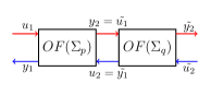
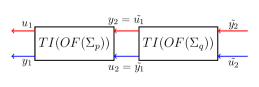
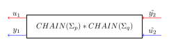
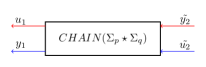
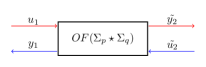
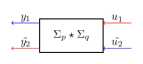
Figure 8: Equivalent system diagrams involving $\operatorname{OF}$ and $\operatorname{TI}$ operators and their composition $\operatorname{CHAIN}=\operatorname{TI}\circ\operatorname{OF}$ of Section III-C. The middle row represents Claim (ii) of Theorem 15. Together with the diagrams in Fig. 7, these constitute the proof of Claim (iii) of Theorem 15 since the same relations between signals $u_{1},u_{2},y_{1},y_{2},\tilde{u}_{1},\tilde{u}_{2},\tilde{y}_{1}$, and $\tilde{y}_{2}$ in all of them.

The system diagrams do not assume even the linearity of the underlying dynamical systems. Extremely complicated networks of dynamical systems can be described in terms of system diagrams ; see, e.g., Fig 8. The parallel and cascade connections of Definition 2 are shown in Fig. 2.

Figure 2: Parallel and cascade connections in terms of system diagrams drawn in standard form. The resulting realisations are denoted by $\Sigma_{p}+\Sigma_{q}$ and $\Sigma_{p}*\Sigma_{q}$ with formulas given in Definition 2.

III-C Fundamental operations of realisations

Figure 3: The representations of the three basic transformations of the original system $\Sigma=\left[\begin{smallmatrix}A&B\\ C&D\end{smallmatrix}\right]$ given in its standard diagrammatic form (top left). The mathematical relations between the signals $u_{1},u_{2},y_{1}$, and $y_{2}$ in all of these systems $\Sigma$, $\operatorname{OF}(\Sigma)$, $\operatorname{TI}(\Sigma)$, and $\operatorname{SR}(\Sigma)$ are by definition the same.

It appears that all couplings and feedback configurations required in this article are combinations of four elementary transformations of the original system $\Sigma=\left[\begin{smallmatrix}A&B\\ C&D\end{smallmatrix}\right]$ described diagrammatically in Fig. 3. In terms of the state space representation of the linear system $\Sigma$, these transformations are as follows:

1. Full Inversion ($\operatorname{FI}$)

   $$\left[\begin{matrix}A&B\\ C&D\end{matrix}\right]=\Sigma\mapsto\operatorname{FI}(\Sigma):=\left[\begin{matrix}A-BD^{-1}C&BD^{-1}\\ -D^{-1}C&D^{-1}\end{matrix}\right].$$ (20)

2. Output Flip ($\operatorname{OF}$)

   $$\left[\begin{matrix}A&B\\ \left[\begin{smallmatrix}C_{1}\\ C_{2}\end{smallmatrix}\right]&\left[\begin{smallmatrix}D_{1}\\ D_{2}\end{smallmatrix}\right]\end{matrix}\right]=\Sigma\mapsto\operatorname{OF}(\Sigma):=\left[\begin{matrix}A&B\\ \left[\begin{smallmatrix}0&I\\ I&0\end{smallmatrix}\right]\left[\begin{smallmatrix}C_{1}\\ C_{2}\end{smallmatrix}\right]&\left[\begin{smallmatrix}0&I\\ I&0\end{smallmatrix}\right]\left[\begin{smallmatrix}D_{1}\\ D_{2}\end{smallmatrix}\right]\end{matrix}\right].$$

3. Top Inversion ($\operatorname{TI}$)

   $$\left[\begin{matrix}A&\left[\begin{smallmatrix}B_{1}&B_{2}\end{smallmatrix}\right]\\ \left[\begin{smallmatrix}C_{1}\\ C_{2}\end{smallmatrix}\right]&\left[\begin{smallmatrix}D_{{11}}&D_{{12}}\\ D_{{21}}&D_{{22}}\end{smallmatrix}\right]\end{matrix}\right]=\Sigma\mapsto\operatorname{TI}(\Sigma):=\left[\begin{matrix}A-B_{1}D_{{11}}^{-1}C_{1}&\left[\begin{smallmatrix}-B_{1}D_{{11}}^{-1}&B_{2}-B_{1}D_{{11}}^{-1}D_{12}\end{smallmatrix}\right]\\ \left[\begin{smallmatrix}-D_{{11}}^{-1}C_{1}\\ C_{2}-D_{{21}}D_{{1}}^{-1}C_{1}\end{smallmatrix}\right]&\left[\begin{smallmatrix}-D_{{11}}^{-1}&-D_{{11}}^{-1}D_{{12}}\\ -D_{{12}}D_{{11}}^{-1}&D_{{22}}-D_{{21}}D_{{11}}^{-1}D_{{12}}\end{smallmatrix}\right]\end{matrix}\right].$$

4. Sign Reversal ($\operatorname{SR}$)

   $$\left[\begin{matrix}A&B\\ \left[\begin{smallmatrix}C_{1}\\ C_{2}\end{smallmatrix}\right]&\left[\begin{smallmatrix}D_{1}\\ D_{2}\end{smallmatrix}\right]\end{matrix}\right]=\Sigma\mapsto\operatorname{SR}(\Sigma):=\left[\begin{matrix}A&B\\ \left[\begin{smallmatrix}I&0\\ 0&-I\end{smallmatrix}\right]\left[\begin{smallmatrix}C_{1}\\ C_{2}\end{smallmatrix}\right]&\left[\begin{smallmatrix}I&0\\ 0&-I\end{smallmatrix}\right]\left[\begin{smallmatrix}D_{1}\\ D_{2}\end{smallmatrix}\right]\end{matrix}\right].$$

The realisation formula for $\operatorname{FI}(\Sigma)$ is called external reciprocal transformation in Section IV-B2. It is the only one of the four transformations that does not require the splitting of inputs to components $u_{1},u_{2}$ or outputs to $y_{1},y_{2}$. Observe that both $\operatorname{FI}(\Sigma)$ and $\operatorname{TI}(\Sigma)$ are only defined for $\Sigma$ for which the result is well-defined.

The compositions of these operations on realisations are denoted by $\circ$. Obviously, $\Sigma=\operatorname{OF}(\operatorname{OF}(\Sigma))=\operatorname{TI}(\operatorname{TI}(\Sigma))=\operatorname{SR}(\operatorname{SR}(\Sigma))$; i.e., $\operatorname{OF}^{-1}=\operatorname{OF}$, $\operatorname{TI}^{-1}=\operatorname{TI}$, and $\operatorname{SR}^{-1}=\operatorname{SR}$. Two further similar operations can be defined in terms of these, namely the Bottom Inversion defined as $\operatorname{BI}:=\operatorname{TI}\circ\operatorname{FI}=\operatorname{FI}\circ\operatorname{TI}$ whose realisation formula is plainly

$$\operatorname{BI}(\Sigma)=\left[\begin{matrix}A-B_{2}D_{{22}}^{-1}C_{2}&\left[\begin{matrix}B_{1}-B_{2}D_{{22}}^{-1}D_{{21}}&-B_{2}D_{{22}}^{-1}\end{matrix}\right]\\ \left[\begin{matrix}C_{1}-D_{{21}}D_{{22}}^{-1}C_{2}\\ -D_{{22}}^{-1}C_{2}\end{matrix}\right]&\left[\begin{matrix}D_{{11}}-D_{{12}}D_{{22}}^{-1}D_{{21}}&-D_{{12}}D_{{22}}^{-1}\\ -D_{{22}}^{-1}D_{{21}}&-D_{{22}}^{-1}\end{matrix}\right]\\ \end{matrix}\right].$$

Clearly, $\operatorname{FI}=\operatorname{TI}\circ\operatorname{BI}=\operatorname{BI}\circ\operatorname{TI}$. The Input Flip given by $\operatorname{IF}:=\operatorname{FI}\circ\operatorname{OF}\circ\operatorname{FI}$ has the realisation formula

$$\left[\begin{matrix}A&B\\ C&D\end{matrix}\right]=\Sigma\mapsto\operatorname{IF}(\Sigma):=\left[\begin{matrix}A&\left[\begin{smallmatrix}B_{1}&B_{2}\end{smallmatrix}\right]\left[\begin{smallmatrix}0&I\\ I&0\end{smallmatrix}\right]\\ C&\left[\begin{smallmatrix}D_{1}&D_{2}\end{smallmatrix}\right]\left[\begin{smallmatrix}0&I\\ I&0\end{smallmatrix}\right]\end{matrix}\right].$$

IV Transformations of realisations

IV-A Internal Cayley and reciprocal transformations

Let $\Sigma=\left[\begin{smallmatrix}A&B\\ C&D\end{smallmatrix}\right]$ be any continuous time system. We define for any $\sigma>0$ the matrices

$$A_{\sigma} :=\left(\sigma+A\right)\left(\sigma-A\right)^{-1},\quad B_{\sigma}:=\sqrt{2\sigma}\left(\sigma-A\right)^{-1}B,$$ (21)

$$C_{\sigma} :=\sqrt{2\sigma}\left(\sigma-A\right)^{-1}C,\quad D_{\sigma}:=D+C\left(\sigma-A\right)^{-1}B=\mathbf{G}_{\Sigma}(\sigma)$$

where $\mathbf{G}_{\Sigma}(\cdot)$ is the transfer function of $\Sigma$. The discrete time system $\phi_{\sigma}=\left(\begin{smallmatrix}A_{\sigma}&B_{\sigma}\\ C_{\sigma}&D_{\sigma}\end{smallmatrix}\right)$ obtained this way is known as the internal Cayley transform of $\Sigma$. The discrete time transfer function of $\phi_{\sigma}$ is given by $\mathbf{D}_{\sigma}(z)=D_{\sigma}+zC_{\sigma}\left(I+zA_{\sigma}\right)^{-1}B_{\sigma}$, and we have the correspondence

$$\mathbf{D}_{\sigma}(z)=\mathbf{G}_{\Sigma}\left(\sigma\frac{1-z}{1+z}\right)\quad\text{for}\quad z\in\mathbb{D}.$$ (22)

Conversely, if $-1\notin\sigma(A_{\sigma})$, we have

$$A =-\sigma\left(I+A_{\sigma}\right)^{-1}\left(I-A_{\sigma}\right),\quad B=\sqrt{2\sigma}\left(I+A_{\sigma}\right)^{-1}B_{\sigma},$$

$$C =\sqrt{2\sigma}C_{\sigma}\left(I+A_{\sigma}\right)^{-1},\quad D=D_{\sigma}-C_{\sigma}(I+A_{\sigma})^{-1}B_{\sigma}$$

since $(\sigma-A)^{-1}=\frac{1}{2\sigma}(I+A_{\sigma})$. The internal Cayley transform can be interpreted as the Crank–Nicolson time discretisation scheme (also known as Tustin’s method) as explained in [14] or as a spectral discretisation method as explained in [23, 24]; see also [15, Section 12.3]. That this time discretisation scheme respects passivity was already indicated in Proposition 7.

It remains to mention the internal reciprocal system $\Sigma_{-}=\left[\begin{smallmatrix}A_{-}&B_{-}\\ C_{-}&D_{-}\end{smallmatrix}\right]$ of $\Sigma=\left[\begin{smallmatrix}A&B\\ C&D\end{smallmatrix}\right]$. If the main operator $A$ is invertible, $\Sigma_{-}$ is defined by

$$A_{-} :=A^{-1},\quad B_{-}:=A^{-1}B,C_{-}:=-CA^{-1},\quad$$ (23)

$$D_{-} :=\mathbf{G}_{\Sigma}(0)=D-CA^{-1}B.$$

Obviously, $\left(\Sigma_{-}\right)_{-}=\Sigma$ and $\mathbf{G}_{\Sigma_{-}}(s)=\mathbf{G}_{\Sigma}\left(1/s\right)$. The reciprocal system is studied in [25],[15, Section 12.4], and it is useful for interchanging high and low frequency contributions in system responses when carrying out dimension reduction based on a desired frequency passband.

IV-B External transformations

Four fundamental operations on state space realisations $\Sigma$ were introduced in Section III-C. Three further combinations of these operations have an essential role in feedbacks of linear dynamical systems. We proceed to introduce them next, and we also discuss further the Full Inversion transformation in Section IV-B2.

Applications produce two variants of linear systems $\Sigma$ that impose different kinds of restriction on couplings of signals: (i) systems whose signals have two different the physical dimensions, and (ii) systems whose signals have the same physical dimensions but different physical directions. Systems of the first kind have transfer functions that typically represent acoustical or electric impedances or admittances. The systems of the second kind transfer energy through their inputs and outputs in three-dimensional space. Both kinds of mathematical systems may be used to describe the same physical configuration but requirements due to, e.g., measurement and instrumentation make different descriptions more preferable.

From now on, we add a purely semantic property to signals in system diagrams: the colour which is either red or blue. System diagrams are always required to satisfy the following colour rule: two signals of different colour cannot be coupled. Depending on the context, the colour of a signal may either refer to the physical dimension or the direction of energy flow in the underlying physics. The colour rule helps keeping track of the underlying physics in the Redheffer star products in Section VI even though mathematics itself is “colour blind”.

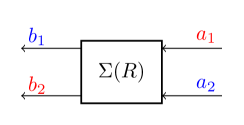
Figure 4: An impedance system with two inputs and two outputs (left). A scattering system $\Sigma(R)$ constructed of $\Sigma_{i}$ with the resistance matrix $R$ (right). The relation between signals is given in Eq. (26). Colour of the signals in left panel refers to the physical dimension and in the right channel to direction of the energy flow.

IV-B1 External Cayley transformations

Let $\Sigma_{i}=\left[\begin{smallmatrix}A_{i}&B_{i}\\ C_{i}&D_{i}\end{smallmatrix}\right]$ be a system whose input and output spaces are $m$-dimensional. Moreover, let $R:=\left[\begin{smallmatrix}R_{1}&0\\ 0&R_{2}\end{smallmatrix}\right]$ be positive, invertible, $m\times m$ resistance matrix. Define now the matrices

$$A :=A_{i}-B_{i}\left(D_{i}+R\right)^{-1}C_{i},\quad B:=\sqrt{2}B_{i}\left(D_{i}+R\right)^{-1}R^{1/2}$$ (24)

$$C :=\sqrt{2}R^{1/2}\left(D_{i}+R\right)^{-1}C_{i},\quad D:=I-2R^{1/2}\left(D_{i}+R\right)^{-1}R^{1/2},$$

comprising the system $\Sigma(R):=\left[\begin{smallmatrix}A&B\\ C&D\end{smallmatrix}\right]$ where it is assumed that $D_{i}+R$ is invertible; see Proposition 9 below. Conversely, we have

$$A_{i} =A+B(I-D)^{-1}C,\quad B_{i}=\sqrt{2}B\left(I-D\right)^{-1}R^{1/2}$$ (25)

$$C_{i} =\sqrt{2}R^{1/2}\left(I-D\right)^{-1}C,\quad D_{i}=R^{1/2}\left(I-D\right)^{-1}\left(I+D\right)R^{1/2}.$$

For reasons explained in Section V, we call $\Sigma_{i}$ and $\Sigma(R)$ the impedance system and scattering system with coupling channel resistance $R$, respectively. Observe that the discretisation parameter $\sigma>0$ in Eq. (21) for the internal Cayley transform and the resistance matrix $R>0$ for the external Cayley transform play somewhat analogous roles.

Any choice of $R>0$ is acceptable for an impedance passive system even though some values of $R$ are more desirable than others:

Proposition 9.

If $\Sigma_{i}=\left[\begin{smallmatrix}A_{i}&B_{i}\\ C_{i}&D_{i}\end{smallmatrix}\right]$ is an impedance passive system, then $\Sigma(R)$ defined by Eq. (24) exists for all invertible $R>0$. Moreover, the feedthrough matrix $D$ of $\Sigma(R)$ satisfies $1\notin\sigma(D)$.

There exists an impedance conservative $\Sigma_{i}$ for which $-1\in\sigma(D)$ since $D_{i}=0$ is possible, and in some physically motivated applications such as Example 1 it is even typical.

Proof.

We have for all $m$-vectors $u$

$$2{\mathrm{R}e\,}\left<(R+D_{i})u,u\right>=\left<(R+D_{i})u,u\right>+\left<u,(R+D_{i})u\right>$$

$$=2\left<Ru,u\right>+\left<(D_{i}+D_{i}^{T})u,u\right>\geq 2\left<Ru,u\right>>0$$

since $D_{i}+D_{i}^{T}\geq 0$ by Proposition 1. Thus $R+D_{i}$ is an invertible $m\times m$ matrix, and the first claim follows. That $1\notin\sigma(D)$ follows from the last equation in Eq. (24). ∎

Denoting the input and output signals of $\Sigma_{i}$ and $\Sigma(R)$ in their dynamical equations (analogously with Eqs. (5)) by $\left[\begin{smallmatrix}i_{1}\\ i_{2}\end{smallmatrix}\right]$, $\left[\begin{smallmatrix}v_{1}\\ v_{2}\end{smallmatrix}\right]$, $\left[\begin{smallmatrix}a_{1}\\ a_{2}\end{smallmatrix}\right]$, $\left[\begin{smallmatrix}b_{1}\\ b_{2}\end{smallmatrix}\right]$, respectively, we have the relations

$$\left[\begin{matrix}a_{1}\\ a_{2}\end{matrix}\right]=\frac{R^{-1/2}}{\sqrt{2}}\left[\begin{matrix}v_{1}+R_{1}i_{1}\\ v_{2}+R_{2}i_{2}\end{matrix}\right]\quad\text{and}\quad\\ \left[\begin{matrix}b_{1}\\ b_{2}\end{matrix}\right]=\frac{R^{-1/2}}{\sqrt{2}}\left[\begin{matrix}v_{1}-R_{1}i_{1}\\ v_{2}-R_{2}i_{2}\end{matrix}\right].$$ (26)

If the physical dimension of $i_{1}$ is current and $v_{1}$ is voltage, then the dimension of $v_{1}+R_{1}i_{1}$ is voltage. It follows, for example, that $\left|a_{1}\right|^{2}=\tfrac{1}{2R_{1}}\left|v_{1}+R_{1}i_{1}\right|^{2}$, and its dimension is thus power. The same holds for the all other signals $a_{2},b_{1},b_{2}$ of the scattering system $\Sigma(R)$.

In practice, both impedance and scattering measurements are used for passive circuits. Direct impedance measurements are impractical for, e.g, high frequency work often carried out using Vector Network Analysers (see, e.g., [26], [27, Section 12]) that are based on scattering parameters instead of voltages and currents. The external Cayley transformation with resistance matrix $R$ is plainly a translation of these frameworks in state space. Scattering systems $\Sigma(R)$ are also directly eligible for Redheffer star products introduced in Section VI.

IV-B2 External reciprocal transformation

The flow inverted system $\Sigma_{f}=\left[\begin{smallmatrix}A_{f}&B_{f}\\ C_{f}&D_{f}\end{smallmatrix}\right]$ of $\Sigma=\left[\begin{smallmatrix}A&B\\ C&D\end{smallmatrix}\right]$ is obtained by $\Sigma_{f}=\operatorname{FI}(\Sigma)$ as introduced in Section III-C. It follows that

$$\mathbf{G}_{\Sigma_{f}}(s)=\mathbf{G}_{\Sigma}(s)^{-1}\,\text{for }s\notin\sigma(A-BD^{-1}C),$$

and we call $\Sigma_{f}$ the external reciprocal transform of $\Sigma$. This transformation is possible if and only if the feedthrough $D$ or, equivalently, $D_{f}$ is an invertible matrix. Indeed, we observe that

$$\begin{cases}x^{\prime}(t)&=A_{f}x(t)+B_{f}y(t),\\ u(t)&=C_{f}x(t)+D_{f}y(t)\end{cases}$$ (27)

holds if and only if Eq. (5) holds. If the transfer function $\mathbf{G}_{\Sigma}(s)$ is an impedance of a passive circuit, then $\mathbf{G}_{\Sigma_{f}}(s)$ is the admittance of the same circuit. From purely mathematical systems theory point of view, the impedance and admittance are completely analogous concepts. However, for some circuits, either impedance, or admittance, or even both of them may not be realisable by a finite-dimensional system which is a restriction on how one should write the modelling equations.

We conclude that the external Cayley and the reciprocal transformations connect systems of scattering, impedance, and admittance type without further restrictions whenever a technical assumption concerning the feedthrough matrix holds:

Proposition 10.

Let $\Sigma=\left[\begin{smallmatrix}A&B\\ C&D\end{smallmatrix}\right]$ be a linear system and $R>0$ be an invertible matrix. Then the following holds:

1. The (impedance) system $\Sigma_{i}=\left[\begin{smallmatrix}A_{i}&B_{i}\\ C_{i}&D_{i}\end{smallmatrix}\right]$ given by Eq. (25) and its external reciprocal transform, the (admittance) system $\left(\Sigma_{i}\right)_{f}$ exist if and only if $\pm 1\notin\sigma(D)$.

2. Defining the (scattering) system $\Sigma(R)$ in terms of $\Sigma_{i}$ and Eqs. (24), we have $\Sigma(R)=\Sigma$.

3. The matrix $D$ is block diagonal in the same way as $R$ if and only if the matrix $D_{i}$ is block diagonal in the same way as $R$.

This follows by inspection of Eq. (25) and the definition of $\Sigma_{f}$.

IV-B3 Hybrid transformation

The two examples given in Section VIII use the external Cayley transformation to produce physically and mathematically realistic Redheffer products. There is yet another way of transforming an impedance passive system $\Sigma_{i}=\left[\begin{smallmatrix}A_{i}&B_{i}\\ C_{i}&D_{i}\end{smallmatrix}\right]$ into the hybrid system $\Sigma_{h}$ (see [6, Example 4.1]) so as to make the Redheffer product of two such (otherwise compatible) systems a physically realistic feedback connection. The corresponding operation for realisations is called the hybrid transformation, which we now introduce for the sake of completeness. The hybrid transformation is illustrated in Fig. 5 in terms of an impedance system

$$\Sigma_{i}=\left[\begin{matrix}A_{i}&\left[\begin{matrix}B_{i_{1}}&B_{i_{2}}\end{matrix}\right]\\ \left[\begin{matrix}C_{i_{1}}\\ C_{i_{2}}\end{matrix}\right]&\left[\begin{matrix}D_{i_{11}}&D_{i_{12}}\\ D_{i_{21}}&D_{i_{22}}\end{matrix}\right]\end{matrix}\right]$$ (28)

associated to differential equations

$$\begin{cases}x^{\prime}(t)&=A_{i}x(t)+B_{i}u(t),\\ y(t)&=C_{i}x(t)+D_{i}u(t)\end{cases}$$ (29)

with the (current) input signal $u(t)=\left[\begin{matrix}i_{1}(t)&i_{2}(t)\end{matrix}\right]^{T}$ and the (voltage) output signal $y(t)=\left[\begin{matrix}v_{1}(t)&v_{2}(t)\end{matrix}\right]^{T}$.

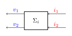
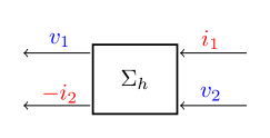
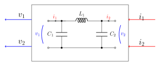
Figure 5: An impedance system $\Sigma_{i}$ (left top panel) and its hybrid transform $\Sigma_{h}$ (right top panel) in diagrammatic form. A $\pi$-topology circuit defining an impedance passive system to be used in Section VIII-A (bottom panel). In all of these diagrams, the relations between $i_{1},i_{2},v_{1},$ and $v_{2}$ are the same. The positive directions of currents in the circuit diagram point always into the circuit, following the convention of Ohm’s law and contrary to the one followed in [27]. When chaining such circuits together using the Redheffer star product, the directions of the currents in couplings must be compatible with Kirchhoff’s laws. This is achieved by including a sign reversal for $i_{2}$ in the hybrid transformation. Recall that the signal arrows in system diagrams separate system inputs from outputs, and they are not related to directions of currents in circuit diagrams.

To compute the realisation for $\Sigma_{h}$ in terms of $\Sigma_{i}$, the new output component $-i_{2}$ is solved from Eqs. (29) which is possible if and only if $D_{i_{22}}$ is invertible. Then the original output component $v_{2}$ becomes an input component. Straightforward computations lead to the realisation

$$\Sigma_{h}=\left[\begin{matrix}A_{i}-B_{i_{2}}D_{i_{22}}^{-1}C_{i_{2}}&\left[\begin{matrix}B_{i_{1}}-B_{i_{2}}D_{i_{22}}^{-1}D_{i_{21}}&B_{i_{2}}D_{i_{22}}^{-1}\end{matrix}\right]\\ \left[\begin{matrix}C_{i_{1}}-D_{i_{21}}D_{i_{22}}^{-1}C_{i_{2}}\\ D_{i_{22}}^{-1}C_{i_{2}}\end{matrix}\right]&\left[\begin{matrix}D_{i_{11}}-D_{i_{12}}D_{i_{22}}^{-1}D_{i_{21}}&D_{i_{12}}D_{i_{22}}^{-1}\\ D_{i_{22}}^{-1}D_{i_{21}}&-D_{i_{22}}^{-1}\end{matrix}\right]\end{matrix}\right].$$ (30)

Recall that the external reciprocal transform $\Sigma_{f}$ of $\Sigma_{i}$ is the full flow inversion given by Eq. (20), and the transfer function of $\Sigma_{f}$ models circuit admittance if $\Sigma_{i}$ is a model for impedance. The hybrid transformation is a partial flow inversion with an extra sign reversal. We leave it to the reader to derive the realisation formula for the inverse hybrid transformation $\Sigma_{h}\mapsto\Sigma_{i}$.

Given $\Sigma_{i}$, both the external Cayley transform $\Sigma(R)$ for $R>0$ and the hybrid transform $\Sigma_{h}$ can, at least in principle, be used for computing Redheffer star products of two systems. It remains to compare these two approaches. Compared to the external Cayley transformation, the benefit of the hybrid transformation is that a resistance matrix $R$ is not required. The invertibility requirement of $D_{i_{22}}$ is quite severe in physically realistic systems whereas any impedance passive $\Sigma_{i}$ has an external Cayley transform $\Sigma(R)$ for any suitable resistance block matrix $R>0$. In fact, the hybrid transformation is unusable for all impedance conservative real finite-dimensional systems with two-dimensional signals as shown in Example 2. Hence, the hybrid transformation is not further developed in this article apart from a few notes.

IV-B4 Chain transformation

It remains to introduce the last transformation of realisations, namely the chain transformation that is introduced in [6, Eq. (4.19) in Section 4.2] for solving the $H^{\infty}$ control problem. The benefit of the chain transformation is that the rather complicated Redheffer star product can be represented as the simple cascade product (see Definition 2) of chain transforms as shown in Theorem 15. We plainly define

$$\operatorname{CHAIN}(\Sigma):=\operatorname{TI}(\operatorname{OF}(\Sigma))\quad\text{for}\quad\Sigma=\left[\begin{matrix}A&\left[\begin{matrix}B_{1}&B_{2}\end{matrix}\right]\\ \left[\begin{matrix}C_{1}\\ C_{2}\end{matrix}\right]&\left[\begin{matrix}D_{{11}}&D_{{12}}\\ D_{{21}}&D_{{22}}\\ \end{matrix}\right]\end{matrix}\right]$$ (31)

whenever the invertibility conditions required by $\operatorname{CHAIN}(\Sigma)$ are satisfied. By direct computations, we get

$$\operatorname{CHAIN}(\Sigma)=\left[\begin{matrix}A-B_{1}D_{21}^{-1}C_{2}&\left[\begin{matrix}B_{2}-B_{1}D_{21}^{-1}D_{22}&B_{1}D_{21}^{-1}\end{matrix}\right]\\ \left[\begin{matrix}C_{1}-D_{11}D_{21}^{-1}C_{2}\\ -D_{21}^{-1}C_{2}\end{matrix}\right]&\left[\begin{matrix}D_{12}-D_{11}D_{21}^{-1}D_{22}&D_{11}D_{21}^{-1}\\ -D_{21}^{-1}D_{22}&D_{21}^{-1}\end{matrix}\right]\end{matrix}\right],$$ (32)

and, hence, $\operatorname{CHAIN}(\Sigma)$ exists if and only if $D_{21}$ is invertible. Conversely, the inverse operation for chain transformation satisfies $\operatorname{CHAIN}^{-1}=\left(\operatorname{TI}\circ\operatorname{OF}\right)^{-1}=\operatorname{OF}^{-1}\circ\operatorname{TI}^{-1}=\operatorname{OF}\circ\operatorname{TI}$. In terms of realisations, we have

$$\operatorname{CHAIN}^{-1}(\Sigma_{c})=\left[\begin{matrix}A_{c}-B_{c_{2}}D_{c_{22}}^{-1}C_{c_{2}}&\left[\begin{matrix}B_{c_{2}}D_{c_{22}}^{-1}&B_{c_{1}}-B_{c_{2}}D_{c_{22}}^{-1}D_{c_{21}}\end{matrix}\right]\\ \left[\begin{matrix}C_{c_{1}}-D_{c_{12}}D_{c_{22}}^{-1}C_{c_{2}}\\ -D_{c_{22}}^{-1}C_{c_{2}}\end{matrix}\right]&\left[\begin{matrix}D_{c_{12}}D_{c_{22}}^{-1}&D_{c_{11}}-D_{c_{12}}D_{c_{22}}^{-1}D_{c_{21}}\\ D_{c_{22}}^{-1}&-D_{c_{22}}^{-1}D_{c_{21}}\end{matrix}\right]\end{matrix}\right]$$ (33)

for

$$\Sigma_{c}=\left[\begin{matrix}A_{c}&\left[\begin{matrix}B_{c_{1}}&B_{c_{2}}\end{matrix}\right]\\ \left[\begin{matrix}C_{c_{1}}\\ C_{c_{2}}\end{matrix}\right]&\left[\begin{matrix}D_{c_{11}}&D_{c_{12}}\\ D_{c_{21}}&D_{c_{22}}\\ \end{matrix}\right]\end{matrix}\right].$$

As pointed out in Section IV-B3, computing Redheffer products is meaningful either for the external Cayley transform $\Sigma(R)$ for $R>0$ or the hybrid transform $\Sigma_{h}$ of an impedance passive $\Sigma_{i}$ splitted as in Eq. (28).

Proposition 11.

Let $\Sigma_{i}$ given by Eq. (28) be an impedance passive system with its external Cayley transform $\Sigma(R)$ for an invertible $R=\left[\begin{smallmatrix}R_{1}&0\\ 0&R_{2}\end{smallmatrix}\right]>0$. By $\Sigma_{h}$ denote the hybrid transform of $\Sigma_{i}$ (if it exists). Then the following holds:

1. $\operatorname{CHAIN}(\Sigma(R))$ exists if and only if $D_{i_{21}}$ is invertible.

2. Both $\Sigma_{h}$ and $\operatorname{CHAIN}(\Sigma_{h})$ exist if and only if both $D_{i_{21}}$ and $D_{i_{22}}$ are invertible.

Proof.

Claim (i): The proof is based on the fact that any block matrix $\left[\begin{smallmatrix}\alpha&\beta\\ \gamma&\delta\end{smallmatrix}\right]$ with square blocks and invertible $\delta$ satisfies

$$\left[\begin{matrix}\alpha&\beta\\ \gamma&\delta\end{matrix}\right]^{-1}=\left[\begin{matrix}(\alpha-\beta\delta^{-1}\gamma)^{-1}&-(\alpha-\beta\delta^{-1}\gamma)^{-1}\beta\delta^{-1}\\ -\delta^{-1}\gamma(\alpha-\beta\delta^{-1}\gamma)^{-1}&(\delta-\gamma\alpha^{-1}\beta)^{-1}\end{matrix}\right]$$

where $\alpha$ and both the Schur complements $\alpha-\beta\delta^{-1}\gamma$ and $\delta-\gamma\alpha^{-1}\beta$ are invertible as a consequence.

By Eq. (24), the feedthrough operator of $\Sigma(R)$ is given by $D=I-2R^{1/2}\left(D_{i}+R\right)^{-1}R^{1/2}$, and we are interested in the bottom left block, say $D_{21}$, of it. Now, $D_{21}$ is invertible if and only if the bottom left block of

$$R^{1/2}\left(D_{i}+R\right)^{-1}R^{1/2}=\left[\begin{matrix}R_{1}^{1/2}&0\\ 0&R_{2}^{1/2}\end{matrix}\right]\left[\begin{matrix}D_{i_{11}}+R_{1}&D_{i_{12}}\\ D_{i_{21}}&D_{i_{22}}+R_{2}\end{matrix}\right]^{-1}\left[\begin{matrix}R_{1}^{1/2}&0\\ 0&R_{2}^{1/2}\end{matrix}\right]$$ (34)

is invertible. Observe that $D_{i}^{T}+D_{i}\geq 0$ by impedance passivity of $\Sigma_{i}$, and $R>0$ is invertible by assumption. The invertibility of $D_{i}+R$ follows as in the proof of Proposition 9. Since $D_{i}^{T}+D_{i}\geq 0$, we have $D_{i_{22}}^{T}+D_{i_{22}}\geq 0$, and hence also $D_{i_{22}}+R_{2}$ is invertible. Since both $R_{1}^{1/2}$ and $R_{2}^{1/2}$ are positive invertible matrices, we only need consider the bottom left block of $(D_{i}+R)^{-1}$ in Eq. (34) which is given by

$$-(D_{i_{22}}+R_{2})^{-1}D_{i_{21}}(D_{i_{11}}+R_{1}-D_{i_{12}}(D_{i_{22}}+R_{2})^{-1}D_{i_{21}})^{-1}$$

using the Schur complements. Its invertibility is equivalent with the invertibility of $D_{i_{21}}$ as claimed.

Claim (ii) is seen to hold by inspection. ∎

It is unfortunate that many physically motivated impedance passive systems have vanishing feedthrough operators $D_{i}=0$ making straightforward chain transformation infeasible. Both of the applications in Section VIII are of this kind.

V Passivity of the transformed systems

The external Cayley transformation is impedance/scattering passivity preserving for any value of the resistance matrix, too.

Proposition 12.

Let $\Sigma(R)=\left[\begin{smallmatrix}A&B\\ C&D\end{smallmatrix}\right]$ and $\Sigma_{i}=\left[\begin{smallmatrix}A_{i}&B_{i}\\ C_{i}&D_{i}\end{smallmatrix}\right]$ be linear systems that are related by Eqs. (24)–(25) where $R>0$ is invertible. Then the following are equivalent:

1. $\Sigma_{i}$ is impedance passive;

2. $\Sigma(R)$ is scattering passive for some invertible $R>0$; and

3. $\Sigma(R)$ is scattering passive for all invertible $R>0$.

The equivalences remain true if the word “passive” is replaced by “conservative”.

Proof.

We prove first the implication (ii) $\Rightarrow$ (i). Let $\tilde{R}>0$ be such that $\Sigma(\tilde{R})=\left[\begin{smallmatrix}\tilde{A}&\tilde{B}\\ \tilde{C}&\tilde{D}\end{smallmatrix}\right]$ is scattering passive where

$$\tilde{A} :=A_{i}-B_{i}\left(D_{i}+\tilde{R}\right)^{-1}C_{i},\quad\tilde{B}:=\sqrt{2}B_{i}\left(D_{i}+\tilde{R}\right)^{-1}\tilde{R}^{1/2}$$

$$\tilde{C} :=\sqrt{2}\tilde{R}^{1/2}\left(D_{i}+\tilde{R}\right)^{-1}C_{i},\quad\tilde{D}:=I-2\tilde{R}^{1/2}\left(D_{i}+\tilde{R}\right)^{-1}\tilde{R}^{1/2}.$$

Because the external Cayley transformation with resistance $R=I$ maps between impedance and scattering passive systems by [18, Theorem 5.2], the system motivated by Eq. (25) with $R=I$

$$\Sigma_{i}(\tilde{R}) =\left[\begin{matrix}\tilde{A}_{i}&\tilde{B}_{i}\\ \tilde{C}_{i}&\tilde{D}_{i}\end{matrix}\right]:=\left[\begin{matrix}\tilde{A}+\tilde{B}(I-\tilde{D})^{-1}\tilde{C}&\sqrt{2}\tilde{B}\left(I-\tilde{D}\right)^{-1}\\ \sqrt{2}\left(I-\tilde{D}\right)^{-1}\tilde{C}&\left(I-\tilde{D}\right)^{-1}\left(I+\tilde{D}\right)\end{matrix}\right]$$ (35)

$$=\left[\begin{matrix}A_{i}&B_{i}\tilde{R}^{-1/2}\\ \tilde{R}^{-1/2}C_{i}&\tilde{R}^{-1/2}D_{i}\tilde{R}^{-1/2}\end{matrix}\right]$$

is impedance passive. Hence,

$$\left[\begin{matrix}\tilde{A}_{i}&\tilde{B}_{i}\\ \tilde{C}_{i}&\tilde{D}_{i}\end{matrix}\right]=\left[\begin{matrix}I&0\\ 0&\tilde{R}^{-1/2}\end{matrix}\right]\left[\begin{matrix}A_{i}&B_{i}\\ C_{i}&D_{i}\end{matrix}\right]\left[\begin{matrix}I&0\\ 0&\tilde{R}^{-1/2}\end{matrix}\right],$$

and it follows from Proposition 1 that $\Sigma_{i}$ is impedance passive.

That (i) $\Rightarrow$ (iii) follows by reading the above given reasoning in converse direction with an arbitrary $R>0$ in place of $\tilde{R}$. The final implication (iii) $\Rightarrow$ (ii) is trivial.

By inspection, the same arguments hold if the word “passive” is consistently replaced by the word “conservative” with the only difference that the LMI in Proposition 1 is then satisfied as equalities. ∎

Proposition 13.

Let $\Sigma=\left[\begin{smallmatrix}A&B\\ C&D\end{smallmatrix}\right]$ be a linear system. Then the following holds:

1. If the internal reciprocal transform $\Sigma_{-}$ of $\Sigma$ exists, it is impedance passive if and only if $\Sigma$ is impedance passive.

2. If the external reciprocal transform $\Sigma_{f}$ of $\Sigma$ exists, it is impedance passive if and only if $\Sigma$ is impedance passive.

Both the claims remain true if the word “passive” is replaced by “conservative”.

Proof.

Claim (i): Recalling Eq. (23), we have

$$\left[\begin{matrix}A_{-}^{T}+A_{-}&B_{-}-C_{-}^{T}\\ B_{-}^{T}-C_{-}&-D_{-}^{T}-D_{-}\end{matrix}\right]=\left[\begin{matrix}A^{-T}+A^{-1}&A^{-1}B+A^{-T}C^{T}\\ B^{T}A^{-T}+CA^{-1}&-D^{T}-D+B^{T}A^{-T}C^{T}+CA^{-1}B\end{matrix}\right].$$

Considering the left hand side, we carry out the following congruence transformation:

$$\left[\begin{matrix}A^{T}&0\\ B^{T}&-I\end{matrix}\right]\begin{bmatrix}A^{-T}+A^{-1}&A^{-1}B+A^{-T}C^{T}\\ B^{T}A^{-T}+CA^{-1}&-D^{T}-D+B^{T}A^{-T}C^{T}+CA^{-1}B\end{bmatrix}\left[\begin{matrix}A&B\\ 0&-I\end{matrix}\right]$$

$$= \left[\begin{matrix}A^{T}&0\\ B^{T}&-I\end{matrix}\right]\begin{bmatrix}A^{-T}A+I&(A^{-T}+A^{-1})B-(A^{-1}B+A^{-T}C^{T})\\ B^{T}A^{-T}A+C&(B^{T}A^{-T}+CA^{-1})B+D^{T}+D-B^{T}A^{-T}C^{T}-CA^{-1}B\end{bmatrix}$$

$$= \left[\begin{matrix}A^{T}&0\\ B^{T}&-I\end{matrix}\right]\begin{bmatrix}A^{-T}A+I&A^{-T}(B-C^{T})\\ B^{T}A^{-T}A+C&D^{T}+D-B^{T}A^{-T}(C^{T}-B)\end{bmatrix}$$

$$= \begin{bmatrix}A+A^{T}&B-C^{T}\\ B^{T}(A^{-T}A+I)-(B^{T}A^{-T}A+C)&B^{T}A^{-T}(B-C^{T})-D^{T}-D+B^{T}A^{-T}(C^{T}-B)\end{bmatrix}$$

$$= \begin{bmatrix}A+A^{T}&B-C^{T}\\ B^{T}-C&-D^{T}-D\end{bmatrix}.$$

Since $\left[\begin{smallmatrix}A_{-}^{T}+A_{-}&B_{-}-C_{-}^{T}\\ B_{-}^{T}-C_{-}&-D_{-}^{T}-D_{-}\end{smallmatrix}\right]$ and $\left[\begin{smallmatrix}A^{T}+A&B-C^{T}\\ B^{T}-C&-D^{T}-D\end{smallmatrix}\right]$ are simultaneously negative or vanish, the claim follows from Proposition 1.

Claim (ii): Now we need to study the block matrix

$$\left[\begin{matrix}A_{f}^{T}+A_{f}&B_{f}-C_{f}^{T}\\ B_{f}^{T}-C_{f}&-D_{f}^{T}-D_{f}\end{matrix}\right]=\left[\begin{matrix}A^{T}-C^{T}D^{-T}B^{T}+A-BD^{-1}C&BD^{-1}+C^{T}D^{-T}\\ D^{-1}C+D^{-T}B^{T}&-D^{-T}-D^{-1}\end{matrix}\right]$$

by Eq. (20). It remains to figure out another congruence transformation:

$$\left[\begin{matrix}I&C^{T}\\ 0&D^{T}\end{matrix}\right]\left[\begin{matrix}A^{T}-C^{T}D^{-T}B^{T}+A-BD^{-1}C&BD^{-1}+C^{T}D^{-T}\\ D^{-1}C+D^{-T}B^{T}&-D^{-T}-D^{-1}\end{matrix}\right]\left[\begin{matrix}I&0\\ C&D\end{matrix}\right]$$

$$= \left[\begin{matrix}I&C^{T}\\ 0&D^{T}\end{matrix}\right]\left[\begin{matrix}A^{T}+A-C^{T}D^{-T}B^{T}-BD^{-1}C+(BD^{-1}+C^{T}D^{-T})C&B+C^{T}D^{-T}D\\ D^{-1}C+D^{-T}B^{T}-(D^{-T}+D^{-1})C&-D^{-T}D-I\end{matrix}\right]$$

$$= \left[\begin{matrix}I&C^{T}\\ 0&D^{T}\end{matrix}\right]\left[\begin{matrix}A^{T}+A-C^{T}D^{-T}B^{T}+C^{T}D^{-T}C&B+C^{T}D^{-T}D\\ D^{-T}(B^{T}-C)&-D^{-T}D-I\end{matrix}\right]$$

$$= \left[\begin{matrix}A^{T}+A-C^{T}D^{-T}(B^{T}-C)+C^{T}D^{-T}(B^{T}-C)&B+C^{T}D^{-T}D+C^{T}(-D^{-T}D-I)\\ B^{T}-C&-D-D^{T}\end{matrix}\right]$$

$$= \left[\begin{matrix}A^{T}+A&B-C^{T}\\ B^{T}-C&-D-D^{T}\end{matrix}\right].$$

Again, $\left[\begin{smallmatrix}A_{f}^{T}+A_{f}&B_{f}-C_{f}^{T}\\ B_{f}^{T}-C_{f}&-D_{f}^{T}-D_{f}\end{smallmatrix}\right]$ and $\left[\begin{smallmatrix}A^{T}+A&B-C^{T}\\ B^{T}-C&-D^{T}-D\end{smallmatrix}\right]$ are simultaneously negative or vanish which completes the proof by Proposition 1. ∎

If the hybrid transform $\Sigma_{h}$ an impedance passive $\Sigma_{i}$ exists, then $\Sigma_{h}$ can be given an equivalent passivity/conservativity notion can be characterised in terms of LMI’s as well. Similarly, the chain transforms $\Sigma_{c}$ of $\Sigma_{h}$ or the scattering passive $\Sigma(R)$, if they exists, can be given such equivalent passivity notions. The conservativity of chain transforms for a (lossless) scattering conservative systems is treated in [6, Chapter 4.4] in terms of $J$-losslessness. Since the mathematical formulations of these variants is immaterial for the purpose of this article, we leave the details for an interested reader.

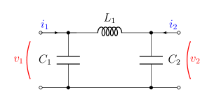
Figure 6: A lossless $\pi$-topology circuit for Example 1, consisting of two capacitances $C_{1},C_{2}$, and one inductance $L_{1}$.

There are elementary physically motivated examples where, e.g., the conditions of Proposition 13 are not satisfied.

Example 1.

The governing equations for the LC circuit shown in Fig. 6 are

$$p_{1}-p_{2}=L_{2}\left(i_{1}-i_{3}\right)^{\prime},\quad p_{1}=\frac{1}{C_{1}}\int_{0}^{t}i_{3}d\tau,\quad\text{and}\quad p_{2}=\frac{1}{C_{3}}\int_{0}^{t}\left(i_{1}+i_{2}-i_{3}\right)d\tau.$$ (36)

By algebraic manipulations, these signals satisfy

$$p_{1}^{\prime}=p_{a},\quad C_{1}p_{a}^{\prime}-i_{1}^{\prime}=\frac{p_{2}-p_{1}}{L_{1}},\quad C_{2}p_{2}^{\prime}=i_{1}+i_{2}-C_{1}p_{a}$$ (37)

where $p_{a}:=p_{1}^{\prime}$. Using the scattering type of signals given in Eq. (26), we get (after carrying out a similarity transformation in the state space) the scattering conservative model $\Sigma(R)=\left[\begin{smallmatrix}A&B\\ C&D\end{smallmatrix}\right]$ for any positive $R:=\left[\begin{smallmatrix}R_{1}&0\\ 0&R_{2}\end{smallmatrix}\right]$ where

$$A:=\left[\begin{matrix}-\frac{1}{{R_{1}}C_{1}}&\frac{1}{\sqrt{{L_{1}}{C_{1}}}}&0\\ -\frac{1}{\sqrt{{L_{1}}{C_{1}}}}&0&\frac{1}{\sqrt{{L_{1}}{C_{2}}}}\\ 0&-\frac{1}{\sqrt{{L_{1}}{C_{2}}}}&-\frac{1}{{R_{2}}{C_{2}}}\end{matrix}\right],\quad B:=\left[\begin{matrix}\sqrt{\frac{2}{R_{1}C_{1}}}&0\\ 0&0\\ 0&\sqrt{\frac{2}{R_{2}C_{2}}}\end{matrix}\right],$$

$C:=B^{T}$, and $D:=-I$. The corresponding impedance system $\Sigma_{i}=\left[\begin{smallmatrix}A_{i}&B_{i}\\ C_{i}&D_{i}\end{smallmatrix}\right]$ can be produced by the inverse external Cayley transformation of Eq. (25) with $D_{i}=0$. The system $\Sigma_{i}$ is impedance conservative by Proposition 1, and $\Sigma(R)$ is then scattering conservative by Proposition 12. This is all of the good news that there are about this example.

The internal reciprocal transform of $\Sigma_{i}$, given by Eq. (23) for $\Sigma(R)$ instead of $\Sigma_{i}$, does not exists since $A_{i}$ given by Eq. (25) is not invertible. The external reciprocal transform of $\Sigma_{i}$, namely the admittance system given by the $\operatorname{FI}$ operation Eq. (20), does not exists since $D_{i}$ is not invertible. Neither does the hybrid system, given by Eq. (30), exist since $(D_{i})_{22}=0$ is not invertible.

Furthermore, the transform $\operatorname{CHAIN}(\Sigma(R))$ does not exists since $D_{21}=0$. Both the internal and external reciprocal transforms of $\Sigma(R)$ exist.

It is instructive to observe that even more general scattering conservative systems with two-dimensional signals can never be transformed to hybrid form assuming that their impedance descriptions are possible to begin with.

Example 2.

Let $\Sigma=\left[\begin{smallmatrix}A&B\\ C&D\end{smallmatrix}\right]$ be a scattering conservative system with $m=2$. Such systems (with real matrices) are characterised by the equations

$$A+A^{T} =-C^{T}C=-BB^{T},\quad D^{T}D=DD^{T}=I,$$ (38)

$$B^{T} =-D^{T}C,\quad C=-DB^{T}.$$

see, e.g., [21, Proposition 1.4]. Then the feedthrough matrix $D\in{\mathbb{R}}^{2\times 2}$ is an orthogonal matrix which is always of one of the following two types:

$$\text{ Either }\qquad S=\begin{bmatrix}\rho&\tau\\ \tau&-\rho\end{bmatrix}\quad\text{(reflection)}\qquad\text{ or }\qquad Q=\begin{bmatrix}\rho&-\tau\\ \tau&\rho\end{bmatrix}\quad\text{(pure rotation)}$$

where $\rho^{2}+\tau^{2}=1$, $\mathop{det}(S)=-1$ (with eigenvalues $\pm 1$), and $\mathop{det}(Q)=1$ (with complex conjugate eigenvalues unless $\tau=0$). Thus, the matrix $D$ has two possibilities: namely,

$$\begin{cases}&\mathop{det}(D)=-1\quad\Rightarrow\quad I-D\text{ is not invertible; or }\\ &\mathop{det}(D)=1\quad\Rightarrow\quad I-D\text{ is invertible if and only if }\rho\in[-1,1).\end{cases}$$

Recalling Eq. (25), we may produce the impedance system $\Sigma_{i}=\left[\begin{smallmatrix}A_{i}&B_{i}\\ C_{i}&D_{i}\end{smallmatrix}\right]$ by the inverse external Cayley transformation only if $\mathop{det}(D)=1$ but $\rho\in[-1,1)$. In this case, $D_{i}$ satisfies

$$D_{i}=(I-D)^{-1}(I+D)=\frac{\tau}{1-\rho}\left[\begin{array}[]{cc}0&-1\\ 1&0\\ \end{array}\right].$$ (39)

(Without loss of generality, we have set $R=I$ in Eq. (25).) For $\rho\in(-1,1)$, the element $\left(D_{i}\right)_{22}=0$ is not invertible (hence, the hybrid transform of $\Sigma_{i}$ does not exist) even though $D_{i}$ is invertible and the admittance system $\Sigma_{f}$ exists since $\tau\neq 0$. Moreover, even $\operatorname{CHAIN}(\Sigma)$ exists for $\rho\in(-1,1)$.

Observe that Example 1 is the special case of Eq. (39) where $\rho=-1$ and $\tau=0$.

Based on Examples 1 and 2, impedance conservative systems $\Sigma_{i}$ in finite dimension may not allow external transformations other than the external Cayley transformation $\Sigma(R)$. Even $\Sigma(R)$ may fail the condition required for defining Redheffer products. A more desirable subclass of impedance passive systems is characterised as follows:

Definition 3.

An impedance passive $\Sigma_{i}=\left[\begin{smallmatrix}A_{i}&B_{i}\\ C_{i}&D_{i}\end{smallmatrix}\right]$ is properly impedance passive if the matrix $D_{i}^{T}+D_{i}\geq 0$ is invertible.

Obviously, the impedance conservative systems, denoted by $\Sigma_{i}$, described in Examples 1 and 2 are impedance passive but not properly so. The external Cayley and reciprocal transforms of a properly impedance passive system have a nice description:

Theorem 14.

Let $\Sigma_{i}=\left[\begin{smallmatrix}A_{i}&B_{i}\\ C_{i}&D_{i}\end{smallmatrix}\right]$ be an impedance passive system whose external Cayley transform $\Sigma(R)=\left[\begin{smallmatrix}A&B\\ C&D\end{smallmatrix}\right]$ is given by Eq. (24) where $R>0$ is invertible. Then the following conditions are equivalent:

1. $\Sigma_{i}$ is properly impedance passive;

2. $\Sigma(R)$ is scattering passive, and the matrix $I-D^{T}D$ is invertible and positive;

3. $\Sigma(R)$ is scattering passive, $\left\|{D}\right\|<1$, and $\sigma(D)\subset\mathbb{D}:=\{z\in\mathbb{C}\,:\,|z|<1\}$ holds;

4. $\Sigma_{i}$ is properly impedance passive, and its feedthrough matrix $D_{i}$ is invertible; and

5. the external reciprocal transform of $\Sigma_{i}$ exists, and it is properly impedance passive.

By Claim (iii) and Propositions 5 and 12, an impedance conservative system cannot be properly impedance passive.

Proof.

(i) $\Leftrightarrow$ (ii): By Proposition (12), $\Sigma_{i}$ is impedance passive if and only if $\Sigma(R)$ is scattering passive. To verify the equivalence, only the feedthrough matrices $D_{i}$ and $D$ remains to be considered. By Proposition 9, the matrix $(I-D)^{-1}$ and its transpose $(I-D^{T})^{-1}$ exist. From Eq. (25) we see that $R^{-1/2}D_{i}R^{-1/2}=\left(I-D\right)^{-1}\left(I+D\right)=I+2D\left(I-D\right)^{-1}=2\left(I-D\right)^{-1}-I$. Thus

$$R^{-1/2}\left(D_{i}^{T}+D_{i}\right)R^{-1/2}=2\left((I-D^{T})^{-1}+(I-D)^{-1}-I\right)$$ (40)

$$=2(I-D^{T})^{-1}\left[(I-D)+(I-D^{T})-(I-D^{T})(I-D)\right](I-D)^{-1}$$

$$=2(I-D^{T})^{-1}\left[2I-D-D^{T}-(I-D-D^{T}+D^{T}D)\right](I-D)^{-1}$$

$$=2(I-D^{T})^{-1}\left[I-D^{T}D\right](I-D)^{-1}.$$

Since the invertibility and positivity of $D_{i}^{T}+D_{i}$ is equivalent with that of $I-D^{T}D$, the equivalence follows.

(ii) $\Rightarrow$ (iii): We have $1\notin\sigma(D)$ by Proposition 9 and $I-D^{T}D\geq 0$ for any scattering passive $\Sigma(R)$. If $I-D^{T}D$ is invertible and nonnegative, the we have $\left\|{u}\right\|>\left\|{Du}\right\|$ for all $u\neq 0$. Since $D$ operates in a finite-dimensional space where the unit ball is compact, we have $\left\|{D}\right\|<1$ and hence $\sigma(D)\subset\mathbb{D}$.

(iii) $\Rightarrow$ (iv): Again, $\Sigma_{i}$ is impedance passive if and only if $\Sigma(R)$ is scattering passive. Since, in particular, $\pm 1\notin\sigma(D)$ holds, the invertibility of $D_{i}$ follows from the last equation in (25). That $D_{i}^{T}+D_{i}$ is invertible follows now from Eq. (40).

(iv) $\Rightarrow$ (v): The external reciprocal transform $\left(\Sigma_{i}\right)_{f}$ exists by claim (ii) and Proposition 10, and its feedthrough matrix is $D_{i}^{-1}$. The system $\left(\Sigma_{i}\right)_{f}$ is impedance passive by claim (ii) of  Proposition 13. Also, the matrix $D_{i}^{T}$ is invertible, and we have $D_{i}^{-T}+D_{i}^{-1}=D_{i}^{-T}\left(D_{i}^{T}+D_{i}\right)D_{i}^{-1}$ where $D_{i}^{T}+D_{i}$ is invertible by assumption. Thus $D_{i}^{-T}+D_{i}^{-1}$ is invertible, and $\left(\Sigma_{i}\right)_{f}$ properly is impedance passive.

(iv) $\Rightarrow$ (i): Trivial.

(v) $\Rightarrow$ (iv): Since $\left(\Sigma_{i}\right)_{f}$ exists, $D_{i}$ is invertible. As the original system satisfies $\Sigma_{i}=\left(\left(\Sigma_{i}\right)_{f}\right)_{f}$, the claim follows from the already proved implication (iv) $\Rightarrow$ (v). ∎

VI Redheffer star product

We proceed to study two-directional feedback couplings. We allow external inputs and outputs in addition to those that are internal to the feedback loop. The fundamental structure of such couplings for systems $\Sigma_{p}$ and $\Sigma_{q}$ is the Redheffer star product $\Sigma_{p}\star\Sigma_{q}$. We will ultimately produce a realisation formula for $\Sigma_{p}\star\Sigma_{q}$ but we first consider it plainly as a feedback configuration shown in Fig. 7.

                 

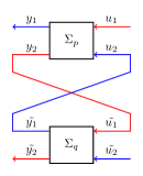
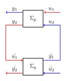
Figure 7: The feedback configuration describing the Redheffer star product $\Sigma_{p}\star\Sigma_{q}$ of systems $\Sigma_{p}$ and $\Sigma_{q}$ diagrammatically drawn in the standard form (left) and an equivalent representation (right). If the systems $\Sigma_{p}$ and $\Sigma_{q}$ are considered as scattering system, the red signals refer to the right going energy wave, and the blue signals refer to the left going energy wave. If the systems are of hybrid form, the colour separates between current and voltage signals.

Starting from impedance passive systems, both the scattering systems in Section IV-B1 and the hybrid systems in Section IV-B3 are eligible for Redheffer star products with other systems of the same kind. We have, in essence, two ways to treat the same feedback connection. The hybrid transformation requires an extra invertibility condition whereas any impedance passive system can be externally Cayley transformed without such restrictions.

However, there are additional requirement on systems $\Sigma_{p}$ and $\Sigma_{q}$ to be suitable for forming the feedback system $\Sigma_{p}\star\Sigma_{q}$. Firstly, the signal pairs $(u_{2},\tilde{y}_{1})$ and $(\tilde{u}_{1},y_{2})$ in Fig. 7 must be of compatible mathematical and physical dimensions. The latter is here reflected by the semantic requirement that the colours of signals in couplings in Fig 7 are not allowed to mix. Also, the feedback loop in Fig. 7 may fail to be well-posed in the sense that it cannot be described by any finite-dimensional state space system at all; see Definition 4 below.

The feedback connection in Fig. 7 alone does not uniquely define a state space for $\Sigma_{p}\star\Sigma_{q}$. Following [6, Chapter 4], it is sometimes possible to compute one state space realisation for $\Sigma_{p}\star\Sigma_{q}$ by reducing it to the cascade product of chain transformed systems; see Definition 2, Section IV-B4, and the following state space variant of [6, Eqs. (4.7)–(4.8) in Section 4.1]:

Theorem 15.

Let

$$\Sigma_{p}=\left[\begin{matrix}A_{p}&\left[\begin{matrix}B_{p_{1}}&B_{p_{2}}\end{matrix}\right]\\ \left[\begin{matrix}C_{p_{1}}\\ C_{p_{2}}\end{matrix}\right]&\left[\begin{matrix}D_{p_{11}}&D_{p_{12}}\\ D_{p_{21}}&D_{p_{22}}\end{matrix}\right]\end{matrix}\right]\qquad\text{ and }\qquad\Sigma_{q}=\left[\begin{matrix}A_{q}&\left[\begin{matrix}B_{q_{1}}&B_{q_{2}}\end{matrix}\right]\\ \left[\begin{matrix}C_{q_{1}}\\ C_{q_{2}}\end{matrix}\right]&\left[\begin{matrix}D_{q_{11}}&D_{q_{12}}\\ D_{q_{21}}&D_{q_{22}}\end{matrix}\right]\end{matrix}\right]$$ (41)

be systems whose signals in Fig. 7 are (dimensionally) feasible for the Redheffer star product $\Sigma_{p}\star\Sigma_{q}$. Assume further that the matrices

$$D_{p_{21}},\quad D_{q_{21}},\quad\text{ and }\quad\Delta_{1}:=I-D_{p_{22}}D_{q_{11}}$$ (42)

are invertible.

1. The chain transforms $\operatorname{CHAIN}(\Sigma_{p})$ and $\operatorname{CHAIN}(\Sigma_{q})$ defined in Eq. (31) exist.

2. There exists a state space realisation, denoted by $\Sigma_{p}\star\Sigma_{q}$, such that $\operatorname{CHAIN}(\Sigma_{p}\star\Sigma_{q})$ exists and satisfies

   $$\operatorname{CHAIN}\left(\Sigma_{p}\star\Sigma_{q}\right)=\operatorname{CHAIN}(\Sigma_{p})*\operatorname{CHAIN}(\Sigma_{q})$$ (43)

   holds where $*$ denotes the cascade product of realisations.

3. The input and output signals of $\Sigma_{p}\star\Sigma_{q}$ have the same relations as the external signals $\left[\begin{smallmatrix}u_{1}\\ \tilde{u}_{2}\end{smallmatrix}\right]$ and $\left[\begin{smallmatrix}y_{1}\\ \tilde{y}_{2}\end{smallmatrix}\right]$ in Fig. 7.

Proof.

Claim (i) follows from the invertibility of $D_{p_{21}}$ and $D_{q_{21}}$; see Eq. (32).

Claim (ii): We see from Eqs. (32)–(33) that the cascade product system $\operatorname{CHAIN}(\Sigma_{p})*\operatorname{CHAIN}(\Sigma_{q})$ is inverse chain transformable. Considering the feedthrough matrices of $\operatorname{CHAIN}(\Sigma_{p})$ and $\operatorname{CHAIN}(\Sigma_{q})$, we get for the feedthrough of $\operatorname{CHAIN}(\Sigma_{p})*\operatorname{CHAIN}(\Sigma_{q})$ the expression

$$\left[\begin{matrix}D_{p_{12}}-D_{p_{11}}D_{p_{21}}^{-1}D_{p_{22}}&D_{p_{11}}D_{p_{21}}^{-1}\\ -D_{p_{21}}^{-1}D_{p_{22}}&D_{p_{21}}^{-1}\end{matrix}\right]\left[\begin{matrix}D_{q_{12}}-D_{q_{11}}D_{q_{21}}^{-1}D_{q_{22}}&D_{q_{11}}D_{q_{21}}^{-1}\\ -D_{q_{21}}^{-1}D_{q_{22}}&D_{q_{21}}^{-1}\end{matrix}\right]$$

$$=\left[\begin{matrix}*&*\\ *&D_{p_{21}}^{-1}\left(I-D_{p_{22}}D_{q_{11}}\right)D_{q_{21}}^{-1}\end{matrix}\right]=\left[\begin{matrix}*&*\\ *&D_{p_{21}}^{-1}\Delta_{1}D_{q_{21}}^{-1}\end{matrix}\right]$$

where the asterisks denote irrelevant entries. By assumptions, the bottom right block is invertible, and this is enough by Eq. (33) to prove the existence of $\Sigma$ such that $\operatorname{CHAIN}\left(\Sigma\right)=\operatorname{CHAIN}(\Sigma_{p})*\operatorname{CHAIN}(\Sigma_{q})$.

Since Claim (iii) concerns only the signals of the feedback system, it would be an unnecessary complication to verify it in terms of state space realisations. Instead, the proof is indicated in terms of system diagrams in Fig. 7 and 8 by reading them from left to right, and from top to bottom. The transformations and the rules of system diagrams given in Section III are used together with the definition $\operatorname{CHAIN}=\operatorname{TI}\circ\operatorname{OF}$.

∎

It remains to present a state space formula for $\Sigma_{p}\star\Sigma_{q}$. Defining $\Sigma_{p}$ and $\Sigma_{q}$ by Eq. (41) and assuming that the matrices Eq. (42) together with $\Delta_{2}:=I-D_{q_{11}}D_{p_{22}}$ are invertible, we get from Eq. (32) and Eq. (43) the expression

$$\Sigma_{p}\star\Sigma_{q}=\left[\begin{matrix}\left[\begin{matrix}A_{11}&A_{12}\\ A_{21}&A_{22}\end{matrix}\right]&\left[\begin{matrix}B_{11}&B_{12}\\ B_{21}&B_{22}\end{matrix}\right]\\ \left[\begin{matrix}C_{11}&C_{12}\\ C_{21}&C_{22}\end{matrix}\right]&\left[\begin{matrix}D_{11}&D_{12}\\ D_{21}&D_{22}\end{matrix}\right]\end{matrix}\right]$$ (44)

where the component block matrices are given by

$$\left[\begin{matrix}A_{11}&A_{12}\\ A_{21}&A_{22}\end{matrix}\right] :=\left[\begin{matrix}A_{p}+B_{p_{2}}\Delta_{2}^{-1}D_{q_{11}}C_{p_{2}}&B_{p_{2}}\Delta_{2}^{-1}C_{q_{1}}\\ B_{q_{1}}\Delta_{1}^{-1}C_{p_{2}}&A_{q}+B_{q_{1}}\Delta_{1}^{-1}D_{p_{22}}C_{q_{1}}\end{matrix}\right]$$ (45)

$$\left[\begin{matrix}B_{11}&B_{12}\\ B_{21}&B_{22}\end{matrix}\right] :=\left[\begin{matrix}B_{p_{1}}+B_{p_{2}}\Delta_{2}^{-1}D_{q_{11}}D_{p_{21}}&B_{p_{2}}\Delta_{2}^{-1}D_{q_{12}}\\ B_{q_{1}}\Delta_{1}^{-1}D_{p_{21}}&B_{q_{2}}+B_{q_{1}}\Delta_{1}^{-1}D_{p_{22}}D_{q_{12}}\end{matrix}\right]$$

$$\left[\begin{matrix}C_{11}&C_{12}\\ C_{21}&C_{22}\end{matrix}\right] :=\left[\begin{matrix}C_{p_{1}}+D_{p_{12}}\Delta_{2}^{-1}D_{q_{11}}C_{p_{2}}&D_{p_{12}}\Delta_{2}^{-1}C_{q_{1}}\\ D_{q_{21}}\Delta_{1}^{-1}C_{p_{2}}&C_{q_{2}}+D_{q_{21}}\Delta_{1}^{-1}D_{p_{22}}C_{q_{1}}\end{matrix}\right]$$

$$\left[\begin{matrix}D_{11}&D_{12}\\ D_{21}&D_{22}\end{matrix}\right] :=\left[\begin{matrix}D_{p_{11}}+D_{p_{12}}\Delta_{2}^{-1}D_{q_{11}}D_{p_{21}}&D_{p_{12}}\Delta_{2}^{-1}D_{q_{12}}\\ D_{q_{21}}\Delta_{1}^{-1}D_{p_{21}}&D_{q_{22}}+D_{q_{21}}\Delta_{1}^{-1}D_{p_{22}}D_{q_{12}}\end{matrix}\right].$$

Observe that $\Delta_{2}^{-1}D_{q_{11}}=D_{q_{11}}\Delta_{1}^{-1}$ and $\Delta_{1}^{-1}D_{p_{22}}=D_{p_{22}}\Delta_{2}^{-1}$ if both $\Delta_{1}$ and $\Delta_{2}$ are invertible. This amounts to some non-uniqueness in how Eqs. (45) can be written.

Remark 1.

It is worth noting that for two systems $\Sigma_{p}$ and $\Sigma_{q}$ with (block) diagonal feedthroughs (consistent with Standing Assumption 2), also $\Sigma_{p}\star\Sigma_{q}$ inherits the same (block) diagonality.

The first observation on Eq. (45) is that the formulas are well-defined even if the matrices $D_{p_{21}}$ and $D_{q_{21}}$ were not invertible. These invertibility assumptions are only required for computing the realisations $\operatorname{CHAIN}(\Sigma_{p})$ and $\operatorname{CHAIN}(\Sigma_{q})$ which is, in fact, not necessary for describing the Redheffer feedback connection itself. Conversely, even if both $\operatorname{CHAIN}(\Sigma_{p})$ and $\operatorname{CHAIN}(\Sigma_{q})$ did exists, the existence of the linear system $\Sigma_{p}\star\Sigma_{q}$ is not always guaranteed through Eqs. (44)–(45) since the invertibility of $\Delta_{1}$ and $\Delta_{2}=I-D_{q_{11}}D_{p_{22}}$ is, in addition, required.

Definition 4.

The feedback loop in Fig. 7 is well-posed if both of the matrices $\Delta_{1}=I-D_{p_{22}}D_{q_{11}}$ and $\Delta_{2}=I-D_{q_{11}}D_{p_{22}}$ in Eq. (42) are invertible.

It is clear from Eq. (44)–(45) that the mappings from the external inputs $(u_{1},\tilde{u}_{2})$ to external outputs $(y_{1},\tilde{y}_{2})$ in Fig. 7 are well-posed (in the sense that their relation can be represented by a transfer function of a finite-dimensional linear system) for invertible $\Delta_{1}$ and $\Delta_{2}$. We may add external perturbations to the feedback loop by setting $u_{2}=\tilde{y}_{1}+v_{2}$ and $\tilde{u}_{1}=y_{2}+\tilde{v}_{1}$, and read the internal outputs $\tilde{y}_{1}$ and $y_{2}$. Even now the mapping $(u_{1},v_{2},\tilde{v}_{1},\tilde{u}_{2})\mapsto(y_{1},y_{2},\tilde{y}_{1},\tilde{y}_{2})$ is similarly well-posed for invertible $\Delta_{1}$ and $\Delta_{2}$.

We need economical conditions to check the well-posedness of the feedback loop.

Lemma 16.

Make the same assumption and use the same notation as in Theorem 15. Necessary conditions for the well-posedness of the feedback loop in Fig. 7 are that

1. the matrices $D_{p_{22}}$ and $D_{q_{11}}$ satisfy $\left\|{D_{p_{22}}}\right\|+\left\|{D_{q_{11}}}\right\|<2$; or

2. one of the matrices $\Delta_{1}$ and $\Delta_{2}$ is invertible.

Proof.

Claim (i) follows because both of the matrices are contractive, and at least one of them strictly so. Thus $\left\|{D_{p_{22}}D_{q_{11}}}\right\|<1$ and $\left\|{D_{q_{11}}D_{p_{22}}}\right\|<1$ implying the invertibility of $\Delta_{1}$ and $\Delta_{2}$ by the usual Neumann series argument.

Claim (ii) follows by showing that $\Delta_{1}$ is invertible if and only if $\Delta_{2}$ is invertible. Assume that the square matrix $\Delta_{1}$ is not invertible, i.e., $\Delta_{1}u=u-D_{p_{22}}D_{q_{11}}u=0$ for some $u\neq 0$. Thus $u=D_{p_{22}}D_{q_{11}}u$, and it follows that $v:=D_{q_{11}}u\neq 0$. Now $v=D_{q_{11}}D_{p_{22}}D_{q_{11}}u=D_{q_{11}}D_{p_{22}}v$ and hence $\Delta_{2}v=0$. We have shown that ${\mathrm{k}er}\left(\Delta_{1}\right)\neq\{0\}$ if and only if ${\mathrm{k}er}\left(\Delta_{2}\right)\neq\{0\}$ which completes the proof. ∎

Proposition 17.

Let $\Sigma_{p}$ and $\Sigma_{q}$ be two scattering passive [conservative] systems such that the feedback loop in Fig. 7 is well-posed. Then the Redheffer star product $\Sigma_{p}\star\Sigma_{q}$ given by Eqs. (44)– (45) is a scattering passive [respectively, conservative] system.

Proof.

Let $\left[\begin{smallmatrix}u_{1}\\ \tilde{u}_{2}\end{smallmatrix}\right]$ be a twice continuously differentiable input signal and $\left[\begin{smallmatrix}x_{p_{0}}\\ x_{q_{0}}\end{smallmatrix}\right]$ an initial state of suitable dimensions for $\Sigma_{p}\star\Sigma_{q}$. It can be seen by a fairly long computation that the Redheffer star product in Eqs. (44)–(45) is so defined that the output signals $y_{1},\tilde{y}_{2}$ and the state trajectories $x_{p},x_{q}$ in the dynamical equations

$$\left[\begin{matrix}x_{p}^{\prime}(t)\\ \left[\begin{matrix}y_{1}(t)\\ y_{2}(t)\end{matrix}\right]\end{matrix}\right]=\Sigma_{p}\left[\begin{matrix}x_{p}(t)\\ \left[\begin{matrix}u_{1}(t)\\ u_{2}(t)\end{matrix}\right]\end{matrix}\right]\quad\text{ and }\quad\left[\begin{matrix}x_{q}^{\prime}(t)\\ \left[\begin{matrix}\tilde{y}_{1}(t)\\ \tilde{y}_{2}(t)\end{matrix}\right]\end{matrix}\right]=\Sigma_{q}\left[\begin{matrix}x_{q}(t)\\ \left[\begin{matrix}\tilde{u}_{1}(t)\\ \tilde{u}_{2}(t)\end{matrix}\right]\end{matrix}\right]\quad\text{ for }t>0$$

with the initial conditions $x_{p}(0)=x_{p_{0}}$, $x_{q}(0)=x_{q_{0}}$ and coupling equations $u_{2}=\tilde{y}_{1},\tilde{u}_{1}=y_{2}$ in Fig. 7 are equivalent with the dynamical equations

$$\left[\begin{matrix}\left[\begin{matrix}x_{p}^{\prime}(t)\\ x_{q}^{\prime}(t)\end{matrix}\right]\\ \left[\begin{matrix}y_{1}(t)\\ \tilde{y}_{2}(t)\end{matrix}\right]\end{matrix}\right]=\Sigma_{p}\star\Sigma_{q}\left[\begin{matrix}\left[\begin{matrix}x_{p}(t)\\ x_{q}(t)\end{matrix}\right]\\ \left[\begin{matrix}u_{1}(t)\\ \tilde{u}_{2}(t)\end{matrix}\right]\end{matrix}\right]\quad\text{ for }t>0$$

with the initial condition $\left[\begin{smallmatrix}x_{p}(0)\\ x_{q}(0)\end{smallmatrix}\right]=\left[\begin{smallmatrix}x_{p_{0}}\\ x_{q_{0}}\end{smallmatrix}\right]$. Since both $\Sigma_{p}$ and $\Sigma_{q}$ are assumed to be scattering passive, their integrated energy inequalities

$$\left\|{x_{p}(T)}\right\|^{2}-\left\|{x_{p_{0}}}\right\|^{2} \leq\int_{0}^{T}{\left(\left\|{u_{1}(t)}\right\|^{2}+\left\|{u_{2}(t)}\right\|^{2}-\left\|{y_{1}(t)}\right\|^{2}-\left\|{y_{2}(t)}\right\|^{2}\right)\,dt}\quad\text{ and }$$

$$\left\|{x_{q}(T)}\right\|^{2}-\left\|{x_{q_{0}}}\right\|^{2} \leq\int_{0}^{T}{\left(\left\|{\tilde{u}_{1}(t)}\right\|^{2}+\left\|{\tilde{u}_{2}(t)}\right\|^{2}-\left\|{\tilde{y}_{1}(t)}\right\|^{2}-\left\|{\tilde{y}_{2}(t)}\right\|^{2}\right)\,dt}$$

hold for all $T$; see Eq. (12). Adding these inequalities and using the coupling equations to cancel out the internal signals gives

$$\left\|{\left[\begin{matrix}x_{p}(T)\\ x_{q}(T)\end{matrix}\right]}\right\|^{2}-\left\|{\left[\begin{matrix}x_{p_{0}}\\ x_{q_{0}}\end{matrix}\right]}\right\|^{2}\leq\int_{0}^{T}{\left(\left\|{\left[\begin{matrix}u_{1}(t)\\ \tilde{u}_{2}(t)\end{matrix}\right]}\right\|^{2}-\left\|{\left[\begin{matrix}y_{1}(t)\\ \tilde{y}_{2}(t)\end{matrix}\right]}\right\|^{2}\right)\,dt}$$

which proves passivity. The proof for conservativity follows by replacing all inequalities in proof with equalities. ∎

Properly impedance passive systems can now be treated through their external Cayley transforms.

Theorem 18.

Let $\Sigma_{p,i}$ and $\Sigma_{q,i}$ be impedance passive systems such that the signals are (dimensionally) compatible as shown in Fig. 7. Assume that at least one of systems $\Sigma_{p,i}$ and $\Sigma_{q,i}$ is properly impedance passive. Define the external Cayley transformed scattering passive systems

$$\Sigma_{p}:=\Sigma_{p,i}(R_{p})\quad\text{ and }\quad\Sigma_{q}:=\Sigma_{q,i}(R_{q})$$

where $R_{p}=\left[\begin{smallmatrix}R_{p,1}&0\\ 0&R_{p,2}\end{smallmatrix}\right]$, $R_{q}=\left[\begin{smallmatrix}R_{q,1}&0\\ 0&R_{q,2}\end{smallmatrix}\right]$ satisfying $R_{p,2}=R_{q,1}$ are invertible, positive resistance matrices. Then the following holds:

1. The internal feedback loop in Fig. 7 is well-posed, and the Redheffer star product $\Sigma_{p}\star\Sigma_{q}$ given by Eqs. (44)–(45) exists.

2. There exists an impedance passive system $\Sigma_{i}^{\prime}$ whose external Cayley transform satisfies $\Sigma^{\prime}(R_{p,q})=\Sigma_{p}\star\Sigma_{q}$ with $R_{p,q}:=\left[\begin{smallmatrix}R_{p,1}&0\\ 0&R_{q,2}\end{smallmatrix}\right]$.

Proof.

We write $\Sigma_{p}=\left[\begin{smallmatrix}A_{p}&B_{p}\\ C_{p}&D_{p}\end{smallmatrix}\right]$ and $\Sigma_{q}=\left[\begin{smallmatrix}A_{q}&B_{q}\\ C_{q}&D_{q}\end{smallmatrix}\right]$ where

$$D_{p}=\left[\begin{matrix}D_{p_{11}}&D_{p_{12}}\\ D_{p_{21}}&D_{p_{22}}\end{matrix}\right]\quad\text{ and }\quad D_{q}=\left[\begin{matrix}D_{q_{11}}&D_{q_{12}}\\ D_{q_{21}}&D_{q_{22}}\end{matrix}\right].$$

To fix notions, we assume that $\Sigma_{p,i}$ properly impedance passive.

Claim (i): We have $\left\|{D_{p}}\right\|<1$ by Theorem 14 and $\left\|{D_{q}}\right\|\leq 1$ by passivity. The claim follow from claim (i) of Lemma 16.

Claim (ii): Considering the feedthrough operator $D:=\left[\begin{smallmatrix}D_{11}&D_{12}\\ D_{21}&D_{22}\end{smallmatrix}\right]$ of $\Sigma_{p}\star\Sigma_{q}$ in Eq. (45), we see that $D\left[\begin{smallmatrix}u_{1}\\ \tilde{u}_{2}\end{smallmatrix}\right]=\left[\begin{smallmatrix}y_{1}\\ \tilde{y}_{2}\end{smallmatrix}\right]$ is equivalent with

$$\left[\begin{matrix}y_{1}\\ y_{2}\end{matrix}\right]=D_{p}\left[\begin{matrix}u_{1}\\ u_{2}\end{matrix}\right],\quad\left[\begin{matrix}\tilde{y}_{1}\\ \tilde{y}_{2}\end{matrix}\right]=D_{q}\left[\begin{matrix}\tilde{u}_{1}\\ \tilde{u}_{2}\end{matrix}\right],\quad u_{2}=\tilde{y}_{1}\quad\text{ and }\quad\tilde{u}_{1}=y_{2}$$ (46)

following the feedback configuration of Fig. 7. For contradiction, assume that $I-D$ is not invertible. Then we must have $D\left[\begin{smallmatrix}u_{1}\\ \tilde{u}_{2}\end{smallmatrix}\right]=\left[\begin{smallmatrix}u_{1}\\ \tilde{u}_{2}\end{smallmatrix}\right]$ for some non-vanishing vector $\left[\begin{smallmatrix}u_{1}\\ \tilde{u}_{2}\end{smallmatrix}\right]$. This together with Eq. (46) gives

$$\left[\begin{matrix}u_{1}\\ \tilde{u}_{1}\end{matrix}\right]=D_{p}\left[\begin{matrix}u_{1}\\ u_{2}\end{matrix}\right],\quad\text{ and }\quad\left[\begin{matrix}u_{2}\\ \tilde{u}_{2}\end{matrix}\right]=D_{q}\left[\begin{matrix}\tilde{u}_{1}\\ \tilde{u}_{2}\end{matrix}\right].$$ (47)

Since $\Sigma_{p,i}$ is properly impedance passive, Theorem 14 implies that $\left\|{D_{p}}\right\|<1$. Since $\Sigma_{q,i}$ is impedance passive, the system $\Sigma_{q}$ is scattering passive satisfying $\left\|{D_{q}}\right\|\leq 1$. Thus, Eq. (47) implies

$$\left\|{u_{1}}\right\|^{2}+\left\|{\tilde{u}_{1}}\right\|^{2}<\left\|{u_{1}}\right\|^{2}+\left\|{u_{2}}\right\|^{2}\quad\text{ and }\quad\left\|{u_{2}}\right\|^{2}+\left\|{\tilde{u}_{2}}\right\|^{2}\leq\left\|{\tilde{u}_{1}}\right\|^{2}+\left\|{\tilde{u}_{2}}\right\|^{2}.$$

Hence $\left\|{\tilde{u}_{1}}\right\|^{2}<\left\|{u_{2}}\right\|^{2}$ and $\left\|{u_{2}}\right\|^{2}\leq\left\|{\tilde{u}_{1}}\right\|^{2}$ which is impossible. We conclude that $I-D$ is invertible, and $\Sigma_{p}\star\Sigma_{q}$ is an external Cayley transform of some $\Sigma_{i}^{\prime}$ by Eq. (25). Moreover, the system $\Sigma_{p}\star\Sigma_{q}$ is scattering passive by Proposition 17, and the impedance passivity of $\Sigma_{i}^{\prime}$ follows from Proposition 12. ∎

VII Regularisation

In finite dimensions, an impedance conservative system $\Sigma_{i}=\left[\begin{smallmatrix}A_{i}&B_{i}\\ C_{i}&D_{i}\end{smallmatrix}\right]$ is characterised by

$$A_{i}+A_{i}^{T}=0,\quad B_{i}^{T}=C_{i},\quad\text{ and }\quad D_{i}+D_{i}^{T}=0$$

by Proposition 1. Because $D_{i}$ does not appear in the first two equations, the system $\Sigma^{\prime}:=\left[\begin{smallmatrix}A_{i}&B_{i}\\ C_{i}&0\end{smallmatrix}\right]$ is impedance conservative if $\Sigma_{i}$ is. A circuit theory example satisfying $D_{i}=0$ is provided in Section 1 below. Thus, the invertibility of $D_{i}$, or any of its parts in splitting $D_{i}=\left[\begin{smallmatrix}D_{i_{11}}&D_{i_{12}}\\ D_{i_{21}}&D_{i_{22}}\end{smallmatrix}\right]$, is not a generic property of impedance conservative systems. Unfortunately, some kind of invertibility is required for computing the external reciprocal transform $\left(\Sigma_{i}\right)_{f}$ by Eq. (20), hybrid transform $\Sigma_{h}$ by Eq. (30), or the chain transform of $\Sigma_{h}$ or $\Sigma(R)$ where $\Sigma(R)$ is the external Cayley transform of $\Sigma_{i}$; see Proposition 11. Even though $\Sigma(R)$ exists and is scattering passive for any impedance passive $\Sigma_{i}$ and $R>0$, the Redheffer product of two such systems may fail to be defined unless the conditions of Lemma 16 are satisfied. Indeed, if $D_{i}=0$ and $\Sigma(R)=\left[\begin{smallmatrix}A&B\\ C&D\end{smallmatrix}\right]$, then $D=-I$ by Eqs. (24) which is an ingredient of a non-well-posed feedback loop.

To compute feedback systems consisting of general impedance passive systems $\Sigma_{i}$, one could take one of these approaches:

1. The external Cayley transform $\Sigma(R)$ of $\Sigma_{i}$ is regularised so as to make the Redheffer star products of such similar systems feasible while preserving scattering passivity.

2. The system $\Sigma_{i}$ is regularised in a way that preserves impedance passivity, so that the hybrid transform $\Sigma_{h}$ and the Redheffer star products of such similar systems are feasible.

Both of these approaches can be taken by using a shift and invert procedure on $\Sigma_{i}$. The first step is the replacement of $D_{i}$ by $D_{i}+\varepsilon I$ for some, purely resistive perturbation $\varepsilon>0$. Clearly $\Sigma_{i}(\varepsilon):=\left[\begin{smallmatrix}A_{i}&B_{i}\\ C_{i}&D_{i}+\varepsilon I\end{smallmatrix}\right]$ is properly impedance passive if $\Sigma_{i}$ is impedance passive by Proposition 1. The second inversion step may be any of the following: (i) the external Cayley transformation, (ii) the hybrid transformation, or even (iii) the external reciprocal transformation, depending on what kind of system is desirable for modelling purposes. In this article, we concentrate on the external Cayley transformation of $\Sigma_{i}(\varepsilon)$, given by

$$\Sigma(R,\varepsilon)=\left[\begin{matrix}A_{i}-B_{i}\left(D_{i}+\varepsilon I+R\right)^{-1}C_{i}&\sqrt{2}B_{i}\left(D_{i}+\varepsilon I+R\right)^{-1}R^{1/2}\\ \sqrt{2}R^{1/2}\left(D_{i}+\varepsilon I+R\right)^{-1}C_{i}&I-2R^{1/2}\left(D_{i}+\varepsilon I+R\right)^{-1}R^{1/2}\end{matrix}\right].$$ (48)

By Theorem 18, the Redheffer star product $\Sigma_{p}\star\Sigma(R,\varepsilon)$ is well-defined for all $\varepsilon>0$ and scattering passive systems $\Sigma_{p}$ such that the feedback loop in Fig. 7 is possible with $\Sigma_{q}=\Sigma(R,\varepsilon)$.

Remark 2.

We have $\lim_{\epsilon\to 0+}{\Sigma(R,\varepsilon)}=\Sigma(R)$ from Eq. (48) where $\Sigma(R)$ is the external Cayley transform of $\Sigma_{i}$. However, it is not as straightforward to make sense of the limit object

$$\lim_{\epsilon\to 0+}\left(\Sigma_{p}\star\Sigma(R,\varepsilon)\right)$$ (49)

for the reason that the natural limit candidate $\Sigma_{p}\star\Sigma(R)$ may not be well-defined by Eqs. (44)–(45). In this case, the matrix elements of $\Sigma_{p}\star\Sigma(R,\varepsilon)$ contain nonnegative powers of $1/\varepsilon$ whose effect on the transfer function of $\Sigma_{p}\star\Sigma(R,\varepsilon)$ may be vanishing as $\epsilon\to 0+$. There does not seem to exist an universal method for describing the limit object in Eq. (49) if the feedback loop of Fig. 7 is not well-posed without regularisation. However, one special case is treated in Section VIII-A.

It is worth noting that Eqs. (45) simplify considerably if $D_{i}$ is (block) diagonal following the splitting of Standing Assumption 2. So as to the system given by Example 1, we get the scattering passive realisation

$$\Sigma(R,\varepsilon)=\left[\begin{matrix}\left[\begin{smallmatrix}\frac{-1}{C_{1}(R_{1}+\varepsilon)}&\frac{1}{\sqrt{L_{1}C_{1}}}&0\\ \frac{-1}{\sqrt{L_{1}C_{1}}}&0&\frac{1}{\sqrt{L_{1}C_{2}}}\\ 0&\frac{1}{\sqrt{L_{1}C_{2}}}&\frac{-1}{C_{2}(R_{2}+\varepsilon)}\end{smallmatrix}\right]&\left[\begin{smallmatrix}\sqrt{\frac{2}{(R_{1}+\varepsilon)C_{1}}}&0\\ 0&0\\ 0&\sqrt{\frac{2}{(R_{2}+\varepsilon)C_{2}}}\end{smallmatrix}\right]\\ \left[\begin{smallmatrix}\sqrt{\frac{2}{(R_{1}+\varepsilon)C_{1}}}&0&0\\ 0&0&\sqrt{\frac{2}{(R_{2}+\varepsilon)C_{2}}}\end{smallmatrix}\right]&\left[\begin{smallmatrix}1-\frac{2R_{1}}{R_{1}+\varepsilon}&0\\ 0&1-\frac{2R_{2}}{R_{2}+\varepsilon}\end{smallmatrix}\right]\end{matrix}\right]\text{ for }\varepsilon>0$$ (50)

where $R=\left[\begin{smallmatrix}R_{1}&0\\ 0&R_{2}\end{smallmatrix}\right]$. We see from this example that the regularisation by shift-and-invert procedure does not make the scattering system chain transformable if the original system is not chain transformable.

VIII Applications

We proceed to give two applications that illuminate the use of realisation techniques for model synthesis. The first application concerns the state space modelling of a passive Butterworth lowpass filter by chaining the LC circuits described in Example 1; see also [13, Section 13.2.5]. The second, more comprehensive application is the one considered in the introduction: an acoustic transmission line, described by the Webster’s PDE (1), is coupled to a load that is modelled by an irrational impedance given in Eq. (4).

VIII-A Passive Butterworth filter in Cauer $\pi$-topology

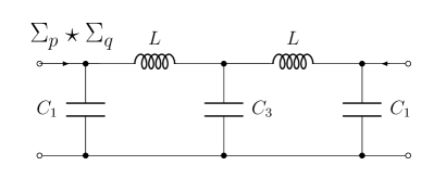
Figure 9: Coupling of two $\pi$-topology circuits whose state space realisations $\Sigma_{p}$ and $\Sigma_{q}$ are derived in Example 1 in scattering form (top panel). When the circuits are coupled corresponding formally to the Redheffer star product $\Sigma_{p}\star\Sigma_{q}$, the two parallel capacitors of value $C_{2}$ can be regarded as a single capacitor of value $C_{3}=2C_{2}$ (bottom panel).

The impedance transfer function of the lossless circuit shown in Fig. 9 is given by

$$Z(s) =\frac{1}{s\left(LC_{1}s^{2}+1\right)\left(LC_{1}C_{3}s^{2}+2C_{1}+C_{3}\right)}\cdot$$ (51)

$$\cdot \left[\begin{matrix}L^{2}C_{1}C_{3}s^{4}+L(2C_{1}+C_{3})s^{2}+1&1\\ 1&L^{2}C_{1}C_{3}s^{4}+L(2C_{1}+C_{3})s^{2}+1\end{matrix}\right].$$

The resonant frequencies of the circuit are given by

$$f_{1}=\frac{1}{2\pi\sqrt{LC_{1}}}\text{ and }f_{2}=\frac{1}{2\pi\sqrt{\tilde{L}\tilde{C}}}\text{ where }\tilde{L}:=\frac{L}{2}\text{ and }\tilde{C}:=\frac{2C_{1}C_{3}}{2C_{1}+C_{3}}.$$ (52)

Since the $\pi$-topology circuit of Example 1 is not properly impedance passive, it is not possible to compute the realisation for the impedance in Eq. (51) by using Theorem 18 without regularisation. However, for any $R=\left[\begin{smallmatrix}R_{0}&0\\ 0&R_{0}\end{smallmatrix}\right]$ and $\varepsilon>0$, the Redheffer star product realisation of the two shift-and-invert regularised component systems takes the form $\Sigma_{p}(R,\varepsilon)\star\Sigma_{q}(R,\varepsilon)=\left[\begin{smallmatrix}A_{\varepsilon}&B_{\varepsilon}\\ C_{\varepsilon}&D_{\varepsilon}\end{smallmatrix}\right]$ where $D_{\varepsilon}=\left[\begin{smallmatrix}1-\frac{2}{\varepsilon+1}&0\\ 0&1-\frac{2}{\varepsilon+1}\end{smallmatrix}\right]$, $C_{\varepsilon}=B_{\varepsilon}^{T}=\left[\begin{smallmatrix}\frac{1}{\varepsilon+R_{0}}\sqrt{\frac{2R_{0}}{C_{1}}}&0&0&0&0&0\\ 0&0&0&0&0&\frac{1}{\varepsilon+R_{0}}\sqrt{\frac{2R_{0}}{C_{1}}}\end{smallmatrix}\right]$, and

$$A_{\varepsilon}=\left[\begin{matrix}-\frac{1}{R_{0}C_{1}{\left(\varepsilon+1\right)}}&\frac{1}{\sqrt{LC_{1}}}&0&0&0&0\\ -\frac{1}{\sqrt{LC_{1}}}&0&\frac{1}{\sqrt{LC_{2}}}&0&0&0\\ 0&-\frac{1}{\sqrt{LC_{2}}}&-\frac{1}{2C_{2}\varepsilon}&\frac{1}{2C_{2}\varepsilon}&0&0\\ 0&0&\frac{1}{2C_{2}\varepsilon}&-\frac{1}{2C_{2}\varepsilon}&\frac{1}{\sqrt{LC_{2}}}&0\\ 0&0&0&-\frac{1}{\sqrt{LC_{2}}}&0&\frac{1}{\sqrt{LC_{1}}}\\ 0&0&0&0&-\frac{1}{\sqrt{LC_{1}}}&-\frac{1}{R_{0}C_{1}{\left(\varepsilon+1\right)}}\end{matrix}\right].$$ (53)

There is a rank one symmetric matrix $A^{\prime}:=\lim_{\eta\to 0}{\eta A_{\eta}}\leq 0$ with eigenvalues $\sigma(A^{\prime}):=\{0,-1/C_{2}\}$, satisfying

$$A_{\varepsilon}=A(\varepsilon)+\frac{A^{\prime}}{\varepsilon}\quad\text{ where }\quad A(0)=\lim_{\varepsilon\to 0}{A(\varepsilon)}\quad\text{ exists. }$$

The realisation $\Sigma_{\varepsilon}:=\Sigma_{p}(R,\varepsilon)\star\Sigma_{q}(R,\varepsilon)$ has a six dimensional state space, yet the circuit in Fig. 9 (bottom panel) has only five components. The capacitor $C_{3}=2C_{2}$ in the circuit of Fig. 9 consists of the two parallel capacitors of capacitance $C_{2}$, each of which corresponds to a separate degree-of-freedom in the state space. Alternatively, one may think that there is an extra pole in the transfer function of $\Sigma_{\varepsilon}$ due to the non-vanishing regularisation parameter $\varepsilon$. In the physically realistic coupling without regularisation (i.e., at the limit $\varepsilon\to 0+$), transfer of charge may take place between each capacitor of value $C_{2}$, resulting in infinite currents in internal conductors of zero resistance inside $C_{3}$. We are dealing with a non-well-posed, yet completely virtual feedback connection in Fig. 9 (bottom panel).

As a first step towards a more economic model, it is possible to give a simplified version of $\Sigma_{\varepsilon}$ for $\varepsilon\approx 0$. Observing that $D_{0}=-I$, $C_{0}=B_{0}^{T}=\left[\begin{smallmatrix}\sqrt{\frac{2}{R_{0}C_{1}}}&0&0&0&0\\ 0&0&0&0&\sqrt{\frac{2}{R_{0}C_{1}}}\end{smallmatrix}\right]$, and defining $A^{\prime}_{\varepsilon}:=A(0)+\frac{A^{\prime}}{\varepsilon}$, we first get the realisation $\Sigma^{\prime}_{\varepsilon}:=\left[\begin{smallmatrix}A^{\prime}_{\varepsilon}&B_{0}\\ C_{0}&D_{0}\end{smallmatrix}\right]$ that is scattering passive for all $\varepsilon>0$. Indeed, all other conditions of scattering conservativity in Proposition 5 are satisfied, except for the Liapunov equation that only holds as the inequality

$$A^{\prime}_{\varepsilon}+\left(A^{\prime}_{\varepsilon}\right)^{*}+C_{0}^{*}C_{0}=A(0)+A(0)^{*}+\frac{2A^{\prime}}{\varepsilon}+C_{0}^{*}C_{0}=\frac{2A^{\prime}}{\varepsilon}\leq 0.$$

The matrix $A^{\prime}_{\varepsilon}$ has two real negative eigenvalues $\lambda_{1}(\varepsilon)$ and $\lambda_{2}(\varepsilon)$ satisfying $\lim_{\varepsilon\to 0+}{\lambda_{1}(\varepsilon)}=-\infty$ and $\lim_{\varepsilon\to 0+}{\lambda_{2}(\varepsilon)}=0$. Also, $\lambda_{1}(\varepsilon)\approx 1/\varepsilon C_{2}$ as $\varepsilon\approx 0$ which is a spurious, transient, and singular (i.e., proportional to $1/\varepsilon$) mode, associated with the regularisation of the non-well-posed feedback loop.

We proceed to entirely removing the spurious eigenvalue $\lambda_{1}(\varepsilon)$ by a structure preserving dimension reduction. Define

$$\tilde{A}:=\left[\begin{matrix}-\frac{1}{R_{0}C_{1}}&\frac{1}{\sqrt{LC_{1}}}&0&0&0\\ -\frac{1}{\sqrt{LC_{1}}}&0&\frac{1}{\sqrt{LC_{3}}}&0&0\\ 0&-\frac{1}{\sqrt{LC_{3}}}&0&\frac{1}{\sqrt{LC_{3}}}&0\\ 0&0&-\frac{1}{\sqrt{LC_{3}}}&0&\frac{1}{\sqrt{LC_{1}}}\\ 0&0&0&-\frac{1}{\sqrt{LC_{1}}}&-\frac{1}{R_{0}C_{1}}\end{matrix}\right]\text{ where }C_{3}=2C_{2},$$

and $\tilde{D}:=-I$, $\tilde{C}:=\tilde{B}^{T}:=\left[\begin{smallmatrix}\sqrt{\frac{2}{R_{0}C_{1}}}&0&0&0&0\\ 0&0&0&0&\sqrt{\frac{2}{R_{0}C_{1}}}\end{smallmatrix}\right]$. Then $\tilde{\Sigma}:=\left[\begin{smallmatrix}\tilde{A}&\tilde{B}\\ \tilde{C}&\tilde{D}\end{smallmatrix}\right]$ is a minimal scattering realisation for the Butterworth filter described by Fig. 9, and it can be obtained by first applying the unitary similarity transformation on $A_{\varepsilon}^{\prime}$ that diagonalises the $2\times 2$ singular block there. Finally, the row and column corresponding to the singular mode $\lambda_{1}(\varepsilon)$ are plainly removed from the original realisation $\Sigma_{\varepsilon}^{\prime}$ to obtain $\tilde{\Sigma}$ without $1/\varepsilon$ dependency.

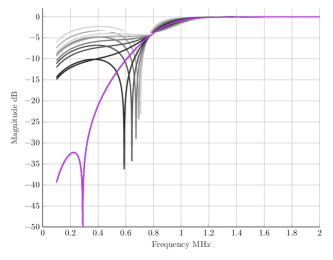
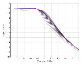
Figure 10: Reflection and transmission parameters $s_{11}$ (left panel) and $s_{21}$ (right panel) of the 5th order Butterworth low pass filter having the topology of Fig. 9. For the cut-off frequency $1\,\mathrm{MHz}$ the approximate component values $C_{1}=2.2\,\mathrm{nF}$, $C_{3}=6.8\,\mathrm{nF}$, and $L=14\,\mu\mathrm{H}$ correspond to matching the $R_{L}=50\,\Omega$ load at both ends. The different versions of $s_{11}$, $s_{21}$ have been computed from the Redheffer realisations $\Sigma_{p}(R,\varepsilon)\star\Sigma_{q}(R,\varepsilon)$ following Eq. (50), using the regularisation parameter value $\varepsilon=1\,\mathrm{n}\Omega$ and $R=R_{0}\left[\begin{smallmatrix}1&0\\ 0&1\end{smallmatrix}\right]$ with $R_{0}/\Omega\in\{20,25,\ldots,50,\ldots 75,80\}$. The curve corresponding $R_{0}=R_{L}$ show least ripple in the passband of $s_{21}$ as expected.

VIII-B Acoustic waveguide terminated to an irrational impedance

We complete the article by modelling an acoustic waveguide that is coupled from one end to an semi-infinite exterior space, modelled by a piston model. Before forming the required Redheffer product in terms of finite-dimensional systems, the acoustic part is spatially discretised by FEM, and the load is rationally approximated by the Löwner’s interpolation method. As an application of this, we compute acoustic signals and frequency responses using anatomic data, acquired by Magnetic Resonance Imaging (MRI) from a test subject during production of vowel $[i]$ as explained in [28].

VIII-B1 Formulating the FEM system

Given continuous and strictly positive functions $k_{1},k_{2}:[0,L]\to{\mathbb{R}}$, consider the partial differential equation for $\phi=\phi(t,\chi)$ satisfying

$$\ddot{\phi}=\frac{1}{k_{1}(\chi)}\frac{\partial}{\partial\chi}\left(k_{2}(\chi)\frac{\partial\phi}{\partial\chi}\right)\quad\text{ for all }\quad\chi\in(0,L)\quad\text{ and }\quad t\geq 0$$ (54)

where $\ddot{\phi}:=\tfrac{\partial^{2}\phi}{\partial t^{2}}$ with the boundary conditions

$$-k_{2}(0)\frac{\partial\phi}{\partial\chi}(t,0) =i_{1}(t)\quad\text{ and }\quad k_{2}(L)\frac{\partial\phi}{\partial\chi}(t,L) =i_{2}(t)\quad\text{ for every }\quad t\geq 0$$ (55)

for continuously differentiable input signals $i_{1}$ and $i_{2}$. The variational formulation of the problem is as follows: Find $\phi=\phi(t,\chi)$, satisfying

$$\phi\in C^{2}([0,\infty);L^{2}(0,L))\cap C^{1}([0,\infty);H^{1}(0,L))\cap C([0,\infty);L^{2}(0,L))$$

such that

$$\frac{\partial^{2}}{\partial t^{2}}\int_{0}^{L}{k_{1}(\chi)\phi(t,\chi)v(\chi)\,\mathrm{d}\chi}+\int_{0}^{L}{k_{2}(\chi)\frac{\partial\phi}{\partial\chi}(t,\chi)\frac{\partial v}{\partial\chi}(\chi)\,\mathrm{d}\chi}$$ (56)

$$=k_{2}(L)\frac{\partial\phi}{\partial\chi}(t,L)v(L)-k_{2}(0)\frac{\partial\phi}{\partial\chi}(t,0)v(0)$$

$$=v(L)i_{2}(t)+v(0)i_{1}(t)$$

for all test functions $v\in H^{1}(0,L)$.

Cubic Hermite Finite Element spaces

Treating the boundary condition such as Eqs. (55)–(56), it is necessary to keep track of spatial derivatives. Instead of the usual piecewise linear approximations, a convenient way of doing this is using a Hermitian Finite Element (FE) space where these derivatives appear as degrees-of-freedom; see, e.g., [29], [30, Section 2.2.3].

Let $\mathcal{C}_{h}$ be a finite family of open, disjoint intervals $(\chi_{i-1},\chi_{i})$ with whose union is dense in $(0,L)$. The notation and enumeration of the nodes $\chi_{i}$ of $\mathcal{C}_{h}$ is given in Fig. 11.

Figure 11: The notation related to the subdivision $\mathcal{C}_{h}$ in the special case of an equidistant division of $[0,L]$.

We make use of the finite-dimensional subspace

$$V_{h}:=\{w\in H^{2}(0,L):w|_{K}\in P_{3}(K)\,\text{ for all }\,K\in\mathcal{C}_{h}\}$$

where $P_{3}(K)$ denotes the space of polynomials of degree $\leq 3$ restricted to $K\subset{\mathbb{R}}$. The Galerkin method applied Eq. (56) gives the following formulation: Find $\phi_{h}\in C^{2}([0,\infty);V_{h})$ such that

$$\frac{\partial^{2}}{\partial t^{2}}\int_{0}^{L}{k_{1}\phi_{h}v_{h}\,\mathrm{d}\chi}+\int_{0}^{L}{k_{2}\frac{\partial\phi_{h}}{\partial\chi}\frac{\partial v_{h}}{\partial\chi}\,\mathrm{d}\chi}\\ =v_{h}(L)i_{2}+v_{h}(0)i_{1}$$ (57)

for all $v_{h}\in V_{h}$. We proceed to construct an explicit basis for $V_{h}$ so as to express Eq. (57) in matrix form.

The local basis functions (see Fig. 12) corresponding to each interval $(\chi_{i-1},\chi_{i})\in\mathcal{C}_{h}$ for $i=1,\ldots,n$, and they are given by

$$\varphi_{i}^{1}(\chi) =2\ell_{i}(\chi)^{3}-3\ell_{i}(\chi)^{2}+1,\quad \varphi_{i}^{2}(\chi)=-2\ell_{i}(\chi)^{3}+3\ell_{i}(\chi)^{2},$$

$$\varphi_{i}^{3}(\chi) =(\ell_{i}(\chi)^{3}-2\ell_{i}(\chi)^{2}+\ell_{i}(\chi))(\chi_{i}-\chi_{i-1}),\qquad \varphi_{i}^{4}(\chi)=(\ell_{i}(\chi)^{3}-\ell_{i}(\chi)^{2})(\chi_{i}-\chi_{i-1})$$

where $\ell_{i}(\chi):=\frac{\chi-\chi_{i-1}}{\chi_{i}-\chi_{i-1}}$. There are two families of global basis functions corresponding to each interior node $\chi_{j}$ for $0<j<n$, and they are given by

$$\psi_{j}^{1}(\chi)=\begin{cases}\varphi_{j}^{2}(\chi),&\text{if $\chi\in(\chi_{j-1},\chi_{j}]$,}\\ \varphi_{j}^{1}(\chi),&\text{if $\chi\in(\chi_{j},\chi_{j+1})$,}\\ 0,&\text{otherwise,}\end{cases}\quad\psi_{j}^{2}(\chi)=\begin{cases}\varphi_{j}^{4}(\chi),&\text{if $\chi\in(\chi_{j-1},\chi_{j}]$,}\\ \varphi_{j}^{3}(x),&\text{if $\chi\in(\chi_{j},\chi_{j+1})$,}\\ 0,&\text{otherwise.}\end{cases}$$

We enumerate these two families as

$$\psi_{k}(\chi) =\begin{cases}\psi_{k}^{1}(\chi),&\text{if}\,\,k\in\{1,\dots,n-1\},\\ \psi_{k-n}^{2}(\chi),&\text{if}\,\,k\in\{n+1,\dots,2n-1\}\end{cases}$$ (58)

which is a basis for $V_{h}\cap H^{1}_{0}(0,L)$. However, solutions $\phi$ of Eq. (54) are expected to have non-trivial Dirichlet traces $\phi(t,0)$ and $\phi(t,L)$. Hence, we need to add the functions

$$\psi_{0}=\varphi_{1}^{1}\quad\text{ and }\quad\psi_{n}=\varphi_{n}^{2}$$ (59)

corresponding the end point nodes $\chi_{0}=0$ and $\chi_{n}=L$, to obtain the basis $\{\psi_{k}\}_{k=0,1,\ldots,2n-1}$ for $V_{h}$; see Fig. 12.

System of linear equations

Since $\phi_{h}(t,\cdot)\in V_{h}$ for all $t\geq 0$, we get using the basis of Eqs. (58)–(59)

$$\phi_{h}(\chi,t)=\sum_{k=0}^{2n-1}{w_{k}(t)\psi_{k}(\chi)}\quad\text{ for }\quad x\in[0,L]\text{ and }t\geq 0$$

where $w_{k}$ are some twice differentiable functions. Writing the coefficient vector $w:=\left[\begin{matrix}w_{0}&\ldots&w_{2n-1}\end{matrix}\right]^{T}\in\mathbb{R}^{2n}$ and the input matrix

$$F:=\left[\begin{matrix}1&0&\ldots&0&0&0&\ldots&0\\ 0&0&\ldots&0&1&0&\ldots&0\end{matrix}\right]^{T}\in\mathbb{R}^{2n\times 2},$$

since $\varphi_{1}^{1}(0)=\varphi_{n}^{2}(L)=1$; here nonzero entries are in the first and $(n+1)$st positions. Eq. (57) takes the form

$$M\ddot{w}(t)+Kw(t)=F\left[\begin{matrix}i_{1}(t)\\ i_{2}(t)\end{matrix}\right],$$ (60)

where $M=\left[\begin{matrix}m_{ij}\end{matrix}\right]$, $K=\left[\begin{matrix}k_{ij}\end{matrix}\right]\in\mathbb{R}^{2n\times 2n}$ are given by

$$m_{ij} =\int_{0}^{L}k_{1}\psi_{j}\psi_{i}\,\mathrm{d}\chi\quad\text{ and }\quad k_{ij} =\int_{0}^{L}{k_{2}\frac{\partial\psi_{j}}{\partial\chi}\frac{\partial\psi_{i}}{\partial\chi}\,\mathrm{d}\chi}.$$

The matrix $M$ is always invertible since the functions $\psi_{j}$ are a basis, but the matrix $K$ is never invertible since constant functions are in $V_{h}$. Defining the extended state trajectory $x=\left[\begin{smallmatrix}w\\ \dot{w}\end{smallmatrix}\right]$, we get following Corollary 3 the equivalent form

$$\dot{x}(t) =A_{i}^{(1)}x(t)+B_{i}^{(1)}\left[\begin{matrix}i_{1}(t)&i_{2}(t)\end{matrix}\right]^{T}\quad\text{ where }$$ (61)

$$A_{i}^{(1)} :=\left[\begin{matrix}0&K^{1/2}M^{-1/2}\\ -M^{-1/2}K^{1/2}&0\end{matrix}\right]\text{ and }B_{i}^{(1)}:=\left[\begin{matrix}0\\ M^{-1/2}F\end{matrix}\right].$$

When modelling acoustics of a variable diameter tube, we have $k_{1}(\chi)=\mathcal{A}(\chi)/c^{2}$ and $k_{2}(\chi)=\mathcal{A}(\chi)$ where $c$ is the speed of sound and $\mathcal{A}(\chi)$ is the cross-sectional area at $\chi\in[0,L]$. The physical dimension of the input signals $i_{1}$ and $i_{2}$ is volume velocity (given in $\mathrm{m}^{3}/\mathrm{s}$). To read out the sound pressures (given in $\mathrm{Pa}$) $p_{1}$ and $p_{2}$ from the system at the ends $\chi=0$ and $\chi=L$ , we define

$$\left[\begin{matrix}p_{1}(t)&p_{2}(t)\end{matrix}\right]^{T}=C_{i}^{(1)}\mathbf{x}(t)\quad\text{ with }C_{i}^{(1)}:=\rho\left[\begin{matrix}0&F^{T}M^{-1/2}\end{matrix}\right]$$ (62)

where the dimension of the zero matrix is $2\times 2n$, and $\rho>0$ denotes the density of the medium. The system defined by Eqs. (61)–(62) is henceforth denoted by $\Sigma_{i}^{(1)}=\left[\begin{smallmatrix}A_{i}^{(1)}&B_{i}^{(1)}\\ C_{i}^{(1)}&0\end{smallmatrix}\right]$. Note that $\Sigma_{i}$ is not yet an impedance conservative system, but impedance conservativity is achieved by dividing $\rho$ in Eq. (62) evenly between $B_{i}^{(1)}$ and $C_{i}^{(1)}$ as $\rho^{1/2}$, see Theorem 2.

Figure 12: The local basis functions $\varphi_{i}^{k}$, $k\in\{1,2,3,4\}$, on the interval $(\chi_{i-1},\chi_{i})=(0,1)$ (left panel). The global basis functions $\psi_{j}^{k}$, $k\in\{1,2\}$, corresponding to the node $\chi_{j}=0.5$ (right panel). In the picture, $\chi_{j-1}=0$ and $x_{j+1}=1$.

VIII-B2 Löwner interpolation of the exterior space impedance

We proceed to construct a low-order model for the acoustics of an unbounded half space in ${\mathbb{R}}^{3}$ as seen from a circular aperture of radius $a>0$. Following the work of Morse and Ingard [1], the acoustic impedance $Z(s)$ from the piston model is given above in Eq. (4). This function satisfies $Z(\overline{s})=\overline{Z(s)}$ and, hence, $Z({\mathbb{R}})\subset{\mathbb{R}}$ for physical reasons. We proceed in two steps: the function $Z(s)$ is first approximated by a rational interpolant using Löwner’s method, and then its McMillan degree is further reduced by the Singular Value Decomposition (SVD).

For a given integer $m>0$, we use two sets of interpolation points $\{\mu_{i}\},\{\lambda_{j}\}\subset\mathbb{C}_{-}$, each having $m$ elements with $\{\mu_{i}\}\cap\{\lambda_{j}\}=\emptyset$. The interpolation data from $Z(s)$ is represented in terms of two $m\times m$ matrices ${\mathbb{L}}=\left[\begin{matrix}l_{ij}\end{matrix}\right]$ and ${\mathbb{M}}=\left[\begin{matrix}m_{ij}\end{matrix}\right]$ given by

$$l_{ij}=\frac{Z(\mu_{i})-Z(\lambda_{j})}{\mu_{i}-\lambda_{j}}\quad\text{ and }\quad m_{ij}=\frac{\mu_{i}Z(\mu_{i})-\lambda_{j}Z(\lambda_{j})}{\mu_{i}-\lambda_{j}}$$

for $1\leq i,j\leq m$ where $2m$ is the total number of interpolation points. Following [31, Chapter 1], we call ${\mathbb{L}}$ and ${\mathbb{M}}$ Löwner and shifted Löwner matrices, respectively. Defining the vectors

$$b:=\left[\begin{matrix}Z(\mu_{1})&Z(\mu_{2})&\ldots&Z(\mu_{m})\end{matrix}\right]^{T}\quad\text{ and }\quad c:=\left[\begin{matrix}Z(\lambda_{1})&Z(\lambda_{2})&\ldots&Z(\lambda_{m})\end{matrix}\right]^{T}$$

we get the linear dynamical system, say $\tilde{\Sigma}_{p}$, given in descriptor form as

$$\begin{cases}{\mathbb{L}}v^{\prime}(t)&={\mathbb{M}}v(t)-bi(t)\\ p(t)&=c^{T}v(t)\end{cases}$$ (63)

whose transfer function is a rational interpolant of values of $Z(s)$ at points $\{\mu_{i}\}\cup\{\lambda_{j}\}$ if the matrix pencil $\left({\mathbb{L}},{\mathbb{M}}\right)$ is regular; see [31, Theorem 1.9], [13, Section 4.5.2].

To avoid complex arithmetics as in [32, Appendix A.2] while respecting the property $Z(\overline{s})=\overline{Z(s)}$, we use interpolation points satisfying in addition to $\{\mu_{i}\}\cap\{\lambda_{j}\}=\emptyset$ and $\{\mu_{i}\}\cup\{\lambda_{j}\}\subset\mathbb{C}\setminus{{\mathbb{R}}}$ the following conditions:

$${\mathbb{L}}\text{ is invertible};\quad\mu_{i}\neq\mu_{j}\text{ and }\lambda_{i}\neq\lambda_{j}\text{ for }i\neq j;\text{ and }$$ (64)

$$\mu_{j+1}=\overline{\mu_{j}}\text{ and }\lambda_{j+1}=\overline{\lambda_{j}}\text{ for odd }j=1,3,\ldots m-1$$

where $m$ even. An unitary change of coordinates given in [32, Appendix A.2] makes it possible to replace matrices ${\mathbb{L}},{\mathbb{M}}$ and vectors $b,c$ in Eq. (63) by their purely real counterparts that are henceforth denoted by the same symbols.

After the construction of real matrices ${\mathbb{L}}$ and ${\mathbb{M}}$ for Eq. (63), the adverse effects of oversampling are removed by reducing their order via SVD following [32, Section 4.2]. More precisely, we write ${\mathbb{L}}=USV^{T}$, and pick left and right singular vectors corresponding to the $k$ largest singular values into $m\times k$ isometric matrices $U_{k}$ and $V_{k}$ with $k\ll m$. The reduced order $k\times k$ matrices ${\mathbb{L}}_{k}=U_{k}^{T}{\mathbb{L}}V_{k}$, ${\mathbb{M}}_{k}=U_{k}^{T}{\mathbb{M}}V_{k}$, and the vectors $B_{i}^{(2)}:=U_{k}^{T}b$, $C_{i}^{(2)}:=cV_{k}^{T}$ define the system $\Sigma_{i}^{(2)}=\left[\begin{smallmatrix}A_{i}^{(2)}&B_{i}^{(2)}\\ \tilde{C}_{i}^{(2)}&0\end{smallmatrix}\right]$ through the dimension reduced equations derived from Eq. (63)

$$\begin{cases}z^{\prime}(t)=A_{i}^{(2)}z(t)+B_{i}^{(2)}i(t)\\ p(t)=C_{i}^{(2)}z(t)\end{cases}$$ (65)

where $A_{i}^{(2)}:={\mathbb{L}}_{k}^{-1}{\mathbb{M}}_{k}$. The external reciprocal transform of $\Sigma_{i}^{(2)}$ is a realisation related to the Dirichlet-to-Neumann map that is used in resonance computations of coupled Helmholtz systems; see, e.g., [33].

VIII-B3 Modelling vowel production

To define the system $\Sigma_{i}^{(i)}$, the cross-section areas $\mathcal{A}(\chi)$ for $\chi\in[0,L]$ are obtained from vocal tract (VT) geometry of a test subject while producing the vowel sound [i] through the process described in [34, 35]. The length of the VT centreline is $L=19.6\,\mathrm{cm}$, and $\chi=0,L$ denote the vocal folds and mouth opening positions, respectively. For spatial discretisation, the equidistant subdivision of $[0,L]$ into $n=99$ subintervals is used, and $A(\chi)$ is considered piecewise linear on this subdivision. The waveguide system $\Sigma_{i}^{(1)}$ is produced as described above, and the dimension of its state space is $4n=396$.

The mouth opening area is used as the parameter $\mathcal{A}_{0}=\mathcal{A}(L)$ for the exterior space impedance $Z(s)$ in Eq. (4). A finite-dimensional system is produced by sampling $Z(s)$ at $2m=300$ interpolation points $\{\mu_{i}\}\cup\{\lambda_{j}\}$ from inside the square $W=\{s\in\mathbb{C}\,:\,0\leq\left|{\mathrm{R}e\,}{s}\right|,\left|{\mathrm{I}m\,}{s}\right|\leq 3\cdot 10^{5}\,\mathrm{rad}/\mathrm{s}\}$ while obeying the restrictions of Eq. (64). Some of the interpolation points are near the zeroes of $Z(s)$, and the rest are uniformly distributed random points. The frequencies under $48\,\mathrm{kHz}$ get accurately modelled in this way. The low-order exterior space model $\Sigma_{i}^{(2)}$ of McMillan degree $k=16$ is obtained by dimension reduction, and the estimated relative error of its transfer function, compared to $|Z(s)|$, is under $3\cdot 10^{-6}\,\mathrm{kg}/\mathrm{m^{4}\,s}$ in the frequency interval of interest. The values $c=343\,\mathrm{m}/\mathrm{s}$ and $\rho=1.225\,\mathrm{kg}/\mathrm{m}^{3}$ are used for both $\Sigma_{i}^{(1)}$ and $\Sigma_{i}^{(2)}$.

To obtain the composite system $\Sigma_{i}=\left[\begin{smallmatrix}A_{i}&B_{i}\\ C_{i}&0\end{smallmatrix}\right]$ (where $A_{i}$ is a $412\times 412$ matrix) and its time discretisation, the following steps are taken:

1. The impedance passive systems $\Sigma_{i}^{(1)}$ and $\Sigma_{i}^{(2)}$ are regularised and externally Cayley transformed to obtain the scattering systems $\Sigma^{(1)}(R)$ and $\Sigma^{(2)}(R_{2},\varepsilon)$ with $R=\left[\begin{smallmatrix}R_{1}&0\\ 0&R_{2}\end{smallmatrix}\right]$ and $R_{1}=R_{2}=1.1\cdot 10^{6}\,\mathrm{kg}/\mathrm{m^{4}\,s}$. The choice of the regularisation parameter $\varepsilon>0$ is discussed below.

2. The Redheffer star product $\Sigma(R_{1},\varepsilon):=\Sigma^{(1)}(R)\star\Sigma^{(2)}(R_{2},\varepsilon)$ is computed to obtain the composite system in scattering form. The system $\Sigma(R_{1},\varepsilon)$ is a scattering passive model for the VT where mouth at $\chi=L$ is coupled to the exterior space, and a virtual control surface right above vocal folds at $\chi=0$ is coupled to a measurement port of load impedance $R_{1}$.

3. The inverse external Cayley transformation (with $R=R_{1}$) is used to obtain the impedance system $\Sigma_{i}(\varepsilon)$ from $\Sigma(R_{1},\varepsilon)$.

4. For time domain simulations by Crank-Nicolson method, the internal Cayley transform $\phi_{\sigma}(\varepsilon)=\left(\begin{smallmatrix}A_{\sigma}&B_{\sigma}\\ C_{\sigma}&D_{\sigma}\end{smallmatrix}\right)$ of $\Sigma_{i}(\varepsilon)$ is computed using $\sigma=88\,200$, corresponding the time discretisation parameter value $h=22.7\mu s$ and the sampling frequency $44\,100\,\mathrm{Hz}$.

The transfer function $\mathbf{G}_{i}(s)=C_{i}\left(s-A_{i}\right)^{-1}B_{i}$ of $\Sigma_{i}(\varepsilon)$ is the computed total acoustic impedance of VT and the exterior space as seen at the vocal folds position. The resonant frequencies $f_{R1},f_{R2},\ldots$, corresponding to the lowest vocal tract formants $F_{1},F_{2},\ldots$, are obtained from the eigenvalues $\lambda\in\sigma(A_{i})$ by $R_{j}={\mathrm{I}m\,}{\lambda_{j}}/2\pi$.

The temporally discretised system $\phi_{\sigma}(\varepsilon)$ is discrete time impedance passive by Proposition 7. To simulate the vowel production in time domain, it needs to be excited by a flow signal waveform, using it as the input to the difference equations Eq. (13) at the sampling frequency of $44\,100\,\mathrm{Hz}$. A suitable flow waveform is provided by the Liljencrantz–Fant (LF) pulse train at $f_{o}=120\,\mathrm{Hz}$ together with the synthesised signals shown in Fig. 13 (left panel) (see also [36, Fig. 4] estimated spectra (middle and right panel). Burg’s method (with model order 100) is used for the data in the middle panel, and an envelope detector is used in the right panel. The spectral tilt over the frequency interval $[200\,\mathrm{Hz},6.4\,\mathrm{kHz}]$ is $\approx-6.5\,\mathrm{dB}/\mathrm{octave}$ in Fig. 13 (middle panel). Considering that losses to VT walls and the glottal opening at $\chi=0$ have been neglected, this value is reasonably consistent with the values $-9.0\ldots-9.2\,\mathrm{dB}/\mathrm{octave}$ that were given in [37, Table 2 on p.15]

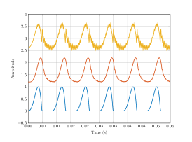
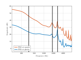
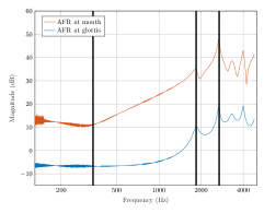
Figure 13: Liljencrantz–Fant (LF) glottal flow excitation waveform at $f_{o}=120\,\mathrm{Hz}$ (left panel, bottom) together with the acoustic pressure waveforms at mouth (middle) and at vocal folds (top) positions as computed from the model. The envelopes of the power spectral densities (using LF excitation) at mouth and vocal folds positions (middle panel). Amplitude frequency responses (using constant amplitude logarithmic sweep) as the input (left panel). All the responses are given without absolute scale.

We complete this work by discussing the accuracy of the low order model $\Sigma_{i}(\varepsilon)$ in terms of measured data. The lowest resonant frequencies, computed from the eigenvalues of $A_{i}$, are $f_{R1}=338\,\mathrm{Hz}$, $f_{R2}=1845\,\mathrm{Hz}$, and $f_{R3}=2693\,\mathrm{Hz}$ using $\varepsilon=0.194\,Z_{0}$ (with $Z_{0}=\rho c/\mathcal{A}_{0}$) as the regularisation parameter for $\Sigma_{i}^{(2)}$ that is tuned to match $f_{R1}\ldots f_{R3}$ to the measured target data $F_{1}\ldots F_{3}$ optimally. As the target data, we use the experimentally obtained formant values $F_{1}\ldots F_{3}$ from vowel samples that were measured from the same test subject in anechoic chamber. These values are $F_{1}=340\pm 25\,\mathrm{Hz}$, $F_{2}=1840\pm 40\,\mathrm{Hz}$, and $F_{3}=2490\pm 60\,\mathrm{Hz}$ as can be read off from [37, Fig. 9]. Obviously, the computed resonant frequencies $f_{R2},f_{R3}$ match the peaks in spectrograms in Fig. 13, extracted from the simulated sound pressure signals at vocal folds and mouth positions.

It is pointed out in [38] that not all formants can always be observed in the power spectrum due to confounding factors; such formant is called latent. Since there is an underlying resonance $f_{R1}$ corresponding to formant $F_{1}$ which is, hence, classified as latent in Fig. 13. Moreover, the model produces no extra spurious resonances under $3\,\mathrm{kHz}$, i.e., resonant frequencies not accounted for by the measurement data on vocal tract replicas [39, Male_i_sweep.pdf in Repository III], nor the speech measurements during MRI [37, Fig. 9], except for those that appear on the negative real axis. Note that $\varepsilon$ can be understood as additional acoustic series resistance to the exterior space model, and it appears that essentially only $f_{R1}$ is sensitive to $\varepsilon$.

Discrepancies between $f_{Rj}$ and $F_{j}$ can be computed from

$$D_{j}=12\log_{2}{\frac{f_{Rj}}{F_{j}}}\quad\text{ in semitones for }j=1,2,3,$$

yielding $D_{1}=-0.1$, $D_{2}=0.05$, and $D_{3}=1.4$, respectively. A computational experiment based on 3D Helmholtz equation was reported in [28, Section 5.2] where the same 3D MRI data was used but the exterior space model was trivial: the homogeneous Dirichlet boundary condition was imposed at the mouth opening. The resulting discrepancies from the computational data of [28, Fig. 7] are $\tilde{D}_{1}=-7.5$, $\tilde{D}_{2}=2.0$, and $\tilde{D}_{3}=2.9$ (accounting for the different speed of sound $c=350\,\mathrm{m}/\mathrm{s}$ used in [28].

We conclude that the proposed 1D acoustics model with only $412$ degrees-of-freedom and an improved treatment of exterior space acoustics produces much better match for $F_{1}\ldots F_{3}$ from experimental data, compared to the 3D Helmholtz FEM solver with $\approx 10^{5}$ degrees-of-freedom.

IX Conclusions

Finite-dimensional realisations have been proposed as a framework for practical numerical modelling of interconnected passive systems. The use of the machinery was illuminated by examples from circuit synthesis and acoustic waveguides.

Under some restrictive assumptions, up to six equivalent reformulations were given in Section IV for the same underlying dynamical system. It is in the nature of things that each of the reformulations make some aspects quite transparent while obscuring other aspects. For example, to write electro-mechanical model equations in continuous time, one is likely to prefer impedance passive formulations in terms of external current and voltage signals satisfying Kirchhoff’s laws in couplings. Continuous time scattering passivity deals with power transmission and reflection parameters satisfying the conservation of energy at the component interfaces, and it is particularly useful for modelling feedback systems as in Section VI. In itself, the characterisation of passivity is easiest for continuous time in impedance setting and for discrete time in scattering setting; see Propositions 1 and 6. It is desirable that spatial discretisation preserves the passivity of the original system, and for some Finite Element discretisations this follows from Theorem 2. Finally, temporal discretisation by Tustin’s method, i.e., the internal Cayley transformation, leads to scattering or impedance passive discrete time systems as given in Proposition 7.

A few words about generalisations that are peripheral to the point of this article. Propositions 1, 5, 6, and 7 are special cases of known infinite-dimensional results on system nodes. Internal transformations in Section IV-A have natural generalisations to system nodes in [15], but the external transformations in Section IV-B require more care because they refer to the feedthrough operator $D$ in an essential way. However, there is a straightforward generalisation to the state-linear systems (see [40]) where $A$ generates a contraction semigroup on a Hilbert state space $X$, with $B,C^{*}\in\mathcal{L}(U;X)$ and $D\in\mathcal{L}(U)$ for the signal Hilbert space $U$. Considering Propositions 9 and 12, the external Cayley transform (with $R=I$) is given in [18, Theorem 5.2] for well-posed (but not necessarily regular) impedance passive system nodes. Furthermore, Propositions 12 and 13 can be generalised to system nodes by usual techniques whereas only a weaker form of Theorem 14 holds even in the case of regular systems where $D$ may be non-compact. Theorems 15 and 18 generalise to state-linear system with finite-dimensional $U$, but both $\Delta_{1}$ and $\Delta_{2}$ need be assumed invertible if $\dim{U}=\infty$. A higher generalisation of the Redheffer star product is, perhaps, easiest obtained by translating to discrete time by the internal Cayley transformation. Finally, Standing Assumption 2 is mostly a matter of convenience, and the signal dimensions in splittings need not generally be the same with the notable exception of the chain transformation where the invertibility of $D_{21}$ is crucial.

Even though state space control is often motivated by the ease of numerical linear algebra compared to the treatment of rational transfer functions, the appeal of realisation techniques is diminished by their inherent numerical burden in large problems. Simulation in discrete time by the internal Cayley transform of $\Sigma=\left[\begin{smallmatrix}A&B\\ C&D\end{smallmatrix}\right]$ can always be arranged so that the matrices in Eq. (21) need not be computed but, instead, a linear problem is solved at each time step. For long time simulations, one would prefer pre-computing the matrices in Eq. (21) if storage is not a concern. So as to external transformations and the Redheffer star product, some resolvents of the feedthrough matrix $D$ of $\Sigma$, or its parts, need be computed at the expense of loss of sparseness. This is a trivial requirement for the examples in Section VIII but increasingly expensive when, e.g., coupling together 3D acoustic subsystems at a common 2D boundary interface. Thus, some form of economy should be exercised in the spatial discretisation of the interfaces connecting the component systems. Alternatively, a special kind of dimension reduction could be used at the interface degrees-of-freedom as was done in [41] for the coupled symmetric eigenvalue problem.

Acknowledgements

JK has received support from Academy of Finland (13312124, 13312340). JM has received support from Magnus Ehrnrooth foundation. TG has received support from Finnish Cultural foundation.

References

- [1] P. Morse and K. Ingard, Theoretical acoustics. McGraw-Hill, 1968.
- [2] M. Abramowitz and I. Stegun, Handbook of Mathematical Functions with Formulas, Graphs, and Mathematical Tables, 9th ed. Dover, 1964.
- [3] J. Malinen and O. Staffans, “Impedance passive and conservative boundary control systems,” Complex Analysis and Operator Theory, vol. 2, no. 1, pp. 279–300, 2007.
- [4] A. Aalto and J. Malinen, “Composition of passive boundary control systems,” Mathematical Control and Related Fields, vol. 3, no. 1, pp. 1–19, 2013.
- [5] A. van der Schaft and D. Jeltsema, Port-Hamiltonian Systems Theory: An Introductory Overview, ser. Foundations and Trends in Systems and Control. The Netherlands: Now Publishers Inc, 2014.
- [6] H. Kimura, Chain-Scattering Approach to -Control, ser. Modern Birkhäuser Classics. Birkhäuser Basel, 1997.
- [7] K. Zhou, J. Doyle, and K. Glover, Robust and optimal control. Prentice Hall, 1996.
- [8] C. Foias and A. Frazho, The commutant lifting approach to interpolation problems, ser. Operator Theory: Advances and applications. Basel, Boston, Berlin: Birkhäuser Verlag, 1990, vol. 44.
- [9] A. Aalto, T. Lukkari, and J. Malinen, “Acoustic wave guides as infinite-dimensional dynamical systems,” ESAIM: Control, Optimisation and Calculus of Variations, vol. 21, no. 2, pp. 324–347, 2015, published online: 17 October 2014.
- [10] J. Makhoul, “Linear prediction: A tutorial review,” Proceedings of the IEEE, vol. 63, no. 4, pp. 561–580, 1975.
- [11] ——, “Spectral linear prediction: Properties and applications,” IEEE Transactions on Acoustics, Speech and Signal Processing, vol. 23, no. 3, pp. 283–296, 1975.
- [12] P. Fuhrmann, Linear systems and operators in Hilbert space. McGraw-Hill, Inc., 1981.
- [13] A. C. Antoulas, Approximation of Large-Scale Dynamical Systems (Advances in Design and Control) (Advances in Design and Control). Philadelphia, PA, USA: Society for Industrial and Applied Mathematics, 2005.
- [14] V. Havu and J. Malinen, “Cayley transform as a time discretization scheme,” Numerical Functional Analysis and Optimization, vol. 28, no. 7, pp. 825–851, 2007.
- [15] O. Staffans, Well-Posed Linear Systems. Cambridge: Cambridge University Press, 2004.
- [16] B. Anderson, Optimal Control. Dover Publications, 2007.
- [17] K. Glover, “All optimal Hankel-norm approximations of linear multivariable systems and their -error bounds,” International Journal of Control, vol. 39, no. 6, pp. 1115–1193, 1984.
- [18] O. Staffans, “Passive and conservative continuous-time impedance and scattering systems. part i: Well-posed systems,” Mathematics of Control, Signals and Systems, vol. 15, no. 4, pp. 291–315, Nov 2002. [Online]. Available: https://doi.org/10.1007/s004980200012
- [19] J. Oostveen and R. Curtain, “Robustly stabilizing controllers for dissipative infinite-dimensional systems with collocated actuators and sensors,” Automatica, vol. 36, no. 3, pp. 337 – 348, 2000. [Online]. Available: http://www.sciencedirect.com/science/article/pii/ S0005109899001697
- [20] G. Weiss and M. Tucsnak, “How to get a conservative well-posed linear system out of thin air. I. Well-posedness and energy balance,” ESAIM. Control, Optimisation and Calculus of Variations, vol. 9, pp. 247–274, 2003.
- [21] J. Malinen, O. Staffans, and G. Weiss, “When is a linear system conservative?” Quarterly of Applied Mathematics, vol. 64, no. 1, pp. 61–91, 2006.
- [22] R. Kalman, P. Falb, and M. Arbib, Topics in Mathematical System Theory, ser. International Series in Pure and Applied Mathematics. McGraw-Hill Book Company, 1969.
- [23] D. Arov and I. Gavrilyuk, “A method for solving initial value problems for linear differential equations in Hilbert space based on the Cayley transform,” Numerical Functional Analysis and Optimization, vol. 14, no. 5&6, pp. 459–473, 1993.
- [24] I. Gavrilyuk and V. Makarov, “The Cayley transform and the solution of an initial value problem for a first order differential equation with an unbounded operator coefficient in Hilbert space,” Numerical Functional Analysis and Optimization, vol. 15, no. 5&6, pp. 583–598, 1994.
- [25] R. Curtain, “Regular linear systems and their reciprocals: applications to riccati equation,” Systems and Control Letters, vol. 49, pp. 81–89, 2003.
- [26] R. Anderson, “S-parameter design for faster, more accurate network design,” Hewlett & Packard Test and Measurement Application Note, vol. 95, no. 1, 1997.
- [27] S. J. Orfanidis, “Electromagnetic waves and antennas,” www.ece.rutgers.edu/ orfanidi/ewa, 2016, last visited 8.11.2018.
- [28] D. Aalto, O. Aaltonen, R.-P. Happonen, P. Jääsaari, A. Kivelä, J. Kuortti, J. M. Luukinen, J. Malinen, T. Murtola, R. Parkkola, J. Saunavaara, and M. Vainio, “Large scale data acquisition of simultaneous MRI and speech,” Applied Acoustics, vol. 83, no. 1, pp. 64–75, 2014.
- [29] Y. Kwon and H. Bang, Finite Element Method Using MATLAB, 1st ed. Boca Raton, FL, USA: CRC Press, Inc., 1996.
- [30] L. Lapidus and G. Pinder, Numerical Solution of Partial Differential Equations in Science and Engineering. Wiley-Interscience, 1999.
- [31] A. Antoulas, C. Beattie, and S. Gugercin, Interpolatory Model Reduction of Large-Scale Dynamical Systems. Springer, 2010, ch. 1.
- [32] A. Ionita and A. Antoulas, “Data-driven parametrized model reduction in the loewner framework,” SIAM Journal on Scientific Computing, vol. 36, no. 3, pp. A984–A1007, 2014.
- [33] J. Araujo-Cabarcas, C. Engström, and E. Jarlebring, “Efficient resonance computations for helmholtz problems based on a dirichlet-to-neumann map,” Journal of Computational and Applied Mathematics, vol. 330, pp. 177 – 192, 2018. [Online]. Available: http://www.sciencedirect.com/science/article/pii/ S0377042717304016
- [34] D. Aalto, J. Helle, A. Huhtala, A. Kivelä, J. Malinen, J. Saunavaara, and T. Ronkka, “Algorithmic surface extraction from MRI data: modelling the human vocal tract,” in Proceedings of BIODEVICES 2013, 2013.
- [35] A. Ojalammi and J. Malinen, “Automated Segmentation of Upper Airways from MRI: Vocal Tract Geometry Extraction,” in BIOIMAGING 2017, Porto, Portugal, 2017, pp. 77–84.
- [36] T. Murtola, A. Aalto, J. Malinen, D. Aalto, and M. Vainio., “Modal locking between vocal fold oscillations and vocal tract acoustics,” Acta Acustica united with Acustica, vol. 104, no. 2, pp. 323–337, 2018.
- [37] J. Kuortti, J. Malinen, and A. Ojalammi, “Post-processing speech recordings during MRI,” Biomedical Signal Processing and Control, vol. 39, pp. 11–22, 2018.
- [38] D. Aalto, J. Malinen, and M. Vainio, “Formants,” Oxford Research Encyclopedia of Linguistics, 2018.
- [39] P. Alku, T. Murtola, J. Malinen, J. Kuortti, B. Story, M. Airaksinen, M. Salmi, E. Vilkman, and A. Geneid, “OPENGLOT – an open environment for the evaluation of glottal inverse filtering,” Speech Communication, vol. 107, pp. 38–47, 2019.
- [40] R. Curtain and H. Zwart, An introduction to infinite-dimensional linear systems theory, ser. Texts in Applied Mathematics. Berlin: Springer Verlag, 1995, vol. 21.
- [41] A. Hannukainen, J. Malinen, and A. Ojalammi, “Efficient solution of symmetric eigenvalue problems from families of coupled systems,” SIAM Journal on Numerical Analysis, vol. 57, no. 4, pp. 1789–1814, 2019.