An $nl$-model with radiative transfer for hydrogen recombination line masers

Abstract

Atomic hydrogen masers occur in recombination plasmas in sufficiently dense H ii regions. These hydrogen recombination line (HRL) masers have been observed in a handful of objects to date and the analysis of the atomic physics involved has been rudimentary. In this work a new model of HRL masers is presented which uses an $nl$-model to describe the atomic populations interacting with free-free radiation from the plasma, and an escape probability framework to deal with radiative transfer effects. The importance of including the collisions between angular momentum quantum states and the free-free emission in models of HRL masers is demonstrated. The model is used to describe the general behaviour of radiative transfer of HRLs and to investigate the conditions under which HRL masers form. The model results show good agreement with observations collected over a broad range of frequencies. Theoretical predictions are made regarding the ratio of recombination lines from the same upper quantum level for these objects.

1 Background

1.1 Hydrogen recombination line masers

Astronomical masers occur when spectral lines are amplified through stimulated emissions and are observed to be much brighter than expected under local thermodynamic equilibrium (LTE) conditions. Molecular astronomical masers have been a very useful tool to probe conditions in a wide variety of sources. Traditional masers are produced by rotational or vibrational transitions in various molecules, but recombination line masers of hydrogen have been discovered in a handful of objects.

Goldberg (1966) showed that recombination lines are amplified by stimulated emissions in the Rayleigh-Jeans limit, even at low optical depths. The theoretical possibility of hydrogen recombination line (HRL) masers was considered by Krolik & McKee (1978) to account for the anomalous hydrogen line intensities found in dense gasses associated with active galactic nuclei. The first cosmic high-gain HRL maser was discovered in the young stellar object MWC 349A (Martin-Pintado et al., 1989a, b). This maser source has since been studied extensively (Planesas et al., 1992; Thum et al., 1992, 1994a, 1994b; Gordon, 1994; Martin-Pintado et al., 1994; Ponomarev, 1994; Thum et al., 1998; Gordon et al., 2001; Weintroub et al., 2008) and the evidence confirms the presence of strongly masing recombination lines.

For some time, MWC 349A was the only source in which HRL masers have been detected, but growing interest in the subject has prompted more searches, leading to the identification of a number of HRL masers in other objects. Masing HRLs have been observed in $\eta$ Carinae (Cox et al., 1995), in a high-velocity ionized jet from the star-forming region Cepheus A HW2 (Jiménez-Serra et al., 2011), from the ultra-compact H ii region Mon R2 (Jiménez-Serra et al., 2013), in the planetary nebula Mz 3 Aleman et al. (2018) and in the gas surrounding the B[e] star MWC 922 (Sánchez Contreras et al., 2017). Because of anomalous H30$\alpha$ line emission, Murchikova et al. (2019) suggest the presence of an HRL maser in the accretion disc around the central Galactic black hole Sgr A^∗. The first extragalactic HRL maser has been detected in the star-forming galaxy NGC 253 (Báez-Rubio et al., 2018). The prospects of using HRL masers on cosmological scales to study the first galaxies (Rule et al., 2013) or the epoch of recombination and reionization (Spaans & Norman, 1997) have been considered.

The environments in which these atomic masers can form are distinctly different from those of their molecular counterparts. For recombination lines to form, the emitting gas has to be ionized. For hydrogen this generally requires a temperature of $\sim 10^{4}$ K. This is the characteristic temperature of a photoionized nebula, which will be the focus of this work. Collisionally ionized gasses can have significantly higher electron temperatures. The host clouds of molecular masers are necessarily cooler than the molecule’s dissociation temperature and therefore are relatively cool. A population inversion occurs in hydrogen over several decades of $n$-levels in a recombination nebula, whereas in molecular masers the inversion is often limited to a few levels. A result of this is that many adjacent HRL lines will exhibit masing behaviour at the same time instead of just a few specific lines as is the case with molecules. In HRL masers, the pumping scheme for the population inversions is a natural consequence of the capture-cascade processes in the atomic component of an ionized gas, which is discussed in more detail in Strelnitski et al. (1996a). In many molecular masers the details associated with the pumping scheme are unclear. It should also be noted that because hydrogen makes up the bulk of almost all astronomical gasses, the masing species can be seen in very high column densities in the case of hydrogen. For molecular masers the relevant constituents have low number densities compared to the H₂ content.

1.2 Challenges of maser modeling

Modeling the interaction between line photons and the emitting matter in an astronomical cloud is key to understanding masers. Such a model will have to account for not only the recombination theory and line formation in multi-level atoms, but also deal with the radiative transfer of the line photons through the cloud. A complete and simultaneous description of both of these components is a complex problem.

A capture-collision-cascade (C³) model, such as the one described by Prozesky & Smits (2018) (hereafter PS18), accounts for the influence that radiation has on atoms in an astronomical cloud by solving the statistical balance equations (SBE) for the level populations of hydrogen. This type of model is appropriate when the plasma is optically thin. When maser action is present, the line radiation is optically thick and radiative transfer effects have to be accounted for. The equation of radiative transfer (ERT) contains the effects that the matter has on the radiation field as it travels through the medium. However, the coefficients in the ERT depend on the local level populations, and the level populations in turn are influenced by the intensity of the radiation field, which is a non-local quantity. This means that these two effects are coupled to one another and, in principle, have to be solved simultaneously in a self-consistent manner to obtain the theoretical intensities of the spectral lines escaping the cloud. Simplifying assumptions, such as the escape probability approximation (EPA) discussed in section 4, are often employed to make the problem tractable.

Hydrogen masers are simpler than molecular masers in the extent that the calculations include all relevant atomic processes to create population inversions. However, hydrogen masers are more complex to model in the sense that several atomic levels that interact directly with one another exhibit masing at the same time. The maser action in hydrogen therefore has a complex effect on the level populations of the participating levels.

1.3 Previous models of HRL masers

There have been some endeavours to construct a theoretical framework for HRL masers. Walmsley (1990) extended the departure coefficient calculations of Brocklehurst & Salem (1977) to higher densities in response to the discovery of the first HRL masing region. Strelnitski et al. (1996a) addressed the theoretical foundations of HRL masers and considered conditions necessary for their formation.

Most theoretical models for HRL masers have focused on the morphology of the emitting region (e.g.​ Ponomarev et al., 1994; Strelnitski et al., 1996b; Weintroub et al., 2008) and it has been suggested that the masing is strongly related to the structure and kinematics of the emitting gas (Martín-Pintado, 2002). Most notable is the three-dimensional non-LTE radiative transfer code MORELI (Báez-Rubio et al., 2013). MORELI uses pre-calculated departure coefficients of either Walmsley (1990) or Storey & Hummer (1995), but does not solve the SBE in a self-consistent way.

Hengel & Kegel (2000) incorporated radiative transfer effects into a C³ model to assess the effects of saturation on the level populations. They employed an $n$-model which neglects the effects of the elastic collisions between angular momentum states, as opposed to an $nl$-model in which they are included. Hengel & Kegel (2000) found that the effects of the radiative transfer on the level populations of hydrogen are important.

1.4 Outline of this paper

Section 2 gives a quick overview of the basic equations involved in radiative transfer theory and establishes the notation used throughout this paper. The importance of including the effects of both the free-free radiation field and elastic collisions for HRL maser models are highlighted in section  3. A summary of the EPA that was used in the current model is given in section 4, as well as a discussion regarding its strengths and limitations. Section 5 outlines the calculational details of the HRL maser model used here. The main results, as well as comparison with observations and predictions are given in section 6. The main conclusions are summarized in section 7.

2 Radiative transfer

The ERT describes the radiation added to and subtracted from a given ray as it travels through a medium and is given by

$$\frac{\mathrm{d}I_{\nu}}{\mathrm{d}l}=-\kappa_{\nu}I_{\nu}+j_{\nu},$$ (1)

where $I_{\nu}$ is the specific intensity and $l$ is the path along the ray. The net (line + continuum) volume emission and absorption coefficients at the frequency $\nu$ are given by $j_{\nu}$ and $\kappa_{\nu}$, respectively. The source function is defined as $S_{\nu}=j_{\nu}/\kappa_{\nu}$.

The total line emission coefficient $j_{nm}$ describes radiation added to the radiation of the spectral line of the transition $n\rightarrow m$ through spontaneous emissions and is defined as

$$j_{nm} =\frac{h\nu}{4\pi}\sum_{l=0}^{n-1}\sum_{l^{{}^{\prime}}=l\pm 1}b_{nl}N_{nl}^{*}A_{nl,ml^{{}^{\prime}}}$$ (2)

where $h$ is Planck’s constant, $b_{nl}$ is the departure coefficient of level $nl$, $N_{nl}^{*}$ is the population of level $nl$ in LTE and $A_{nl,ml^{{}^{\prime}}}$ is the Einstein A-value for the $nl\rightarrow ml^{{}^{\prime}}$ transition.

The total line absorption coefficient $\kappa_{mn}$ gives the contribution of stimulated emissions ($B_{nm}$) and absorptions ($B_{mn}$) to the emerging radiation field as

$$\kappa_{mn} =\frac{h\nu}{4\pi}\left(N_{m}B_{mn}-N_{n}B_{nm}\right)$$ (3)

$$=\frac{h\nu}{4\pi}\sum_{l=0}^{n-1}\sum_{l^{{}^{\prime}}=l\pm 1}b_{ml^{{}^{\prime}}}N^{*}_{ml^{{}^{\prime}}}B_{ml^{{}^{\prime}},nl}\left(1-\frac{b_{nl}}{b_{ml^{{}^{\prime}}}}\mathrm{e}^{-h\nu/kT_{\mathrm{e}}}\right)\,,$$ (4)

where $k$ is the Boltzmann constant and $T_{\mathrm{e}}$ is the temperature of the free electron gas, which is assumed to have a Maxwellian distribution.

From the definition in equation (3), it is clear that $\kappa_{mn}$ can become negative if the number of stimulated emissions exceeds the number of absorptions, thereby increasing the line intensity. The term inside brackets in equation (4) is the correction for stimulated emission.

Each transition has a well defined frequency $\nu_{nm}$ associated with it, but in practice there is a range of frequencies around $\nu_{nm}$ where photons from the line transition can be either emitted or absorbed. The emission and absorption coefficients at any particular frequency within the line are described by

$$j_{nm}^{\nu}=j_{nm}\phi_{\nu}\quad\mathrm{and}\quad\kappa_{mn}^{\nu}=\kappa_{mn}\phi_{\nu}\,.$$ (5)

Strictly speaking, the line profile functions $\phi_{\nu}$ for emissions and absorptions are not equal, but they are similar enough for the purposes of this discussion that they will be considered to be equal.

At low enough frequencies, when the continuum is significant which usually occurs in the Rayleigh-Jeans limit, the line and continuum radiation are formed together. This means the net quantities (indicated by subscripts $\nu$) in equation (1) must take into account the contributions of both the line radiation and the continuum (indicated by subscripts $\mathrm{c}$), so that

$$\kappa_{\nu}=\kappa_{mn}^{\nu}+\kappa_{\mathrm{c}},\qquad j_{\nu}=j_{nm}^{\nu}+j_{\mathrm{c}}\,.$$ (6)

The net source function $S_{\nu}$ is given by

$$S_{\nu}=\frac{j_{nm}^{\nu}+j_{\mathrm{c}}}{\kappa_{mn}^{\nu}+\kappa_{\mathrm{c}}}\,.$$ (7)

For a homogeneous medium of thickness $L$ the optical depth is given by

$$\tau_{\nu}=-L\kappa_{\nu}\,.$$ (8)

It is usual to calculate the line intensity at a specific frequency by subtracting the continuum from the total intensity using

$$\bar{J}^{\nu}_{nm}=S_{\nu}\left(1-e^{-\tau_{\nu}}\right)-B_{\nu}\left(1-e^{-\tau_{\mathrm{c}}}\right)\,,$$ (9)

where $B_{\nu}$ is the Planck distribution function, see for example Goldberg (1966) and Strelnitski et al. (1996a). However, if the gas becomes optically thick, the continuum photons will interact with the atoms in a significant way so that the contribution of the line photons to the total intensity at line centre is

$$J_{nm}^{\nu}=\left(\frac{j_{nm}^{\nu}}{\kappa_{mn}^{\nu}+\kappa_{\mathrm{c}}}\right)\left(1-e^{-\tau_{\nu}}\right)\,.$$ (10)

Similarly, the contribution of the continuum photons will be

$$J_{\mathrm{c}}^{\nu}=\left(\frac{j_{\mathrm{c}}}{\kappa_{mn}^{\nu}+\kappa_{\mathrm{c}}}\right)\left(1-e^{-\tau_{\nu}}\right)\,.$$ (11)

Equations (10) and (11) account for the fact that the mean free path of a photon depends only on its frequency, not on its origin. The line intensity $J_{nm}^{\nu}$ described by equation (10) cannot be measured directly from a spectrum. Therefore the quantity $\bar{J}^{\nu}_{nm}$ described by equation (9) will be referred to as the observable line intensity under optically thick conditions.

From an observational perspective, the quantity described by equation (9) can be extracted from an observed spectrum, even if the radiation is emitted from an optically thick region where maser effects are important. A comparison between the behaviour of $\bar{J}^{\nu}_{nm}$ and $J_{nm}^{\nu}$ is discussed in section 6.2.

In our models, the continuum absorption coefficient $\kappa_{\mathrm{c}}$ in the Rayleigh-Jeans regime is calculated using the expression of Oster (1961) given by

$$\kappa_{\mathrm{c}}=\left(\frac{N_{\mathrm{e}}N_{\mathrm{i}}}{\nu^{2}}\right)\left(\frac{8Z^{2}e^{6}}{3\sqrt{3}m_{\mathrm{e}}^{3}c}\right)\left(\frac{\pi}{2}\right)^{1/2}\left(\frac{m_{\mathrm{e}}}{kT_{\mathrm{e}}}\right)^{3/2}\left\langle g\right\rangle\,,$$ (12)

where $N_{\mathrm{e}}$ and $N_{\mathrm{i}}$ are the number densities of the electrons and ions, $Z$ is the atomic charge, $e$ is the elementary charge, $m_{\mathrm{e}}$ is the electron mass, and $c$ is the speed of light. For $T_{\mathrm{e}}<550\,000$ K, the Gaunt factor averaged over a Maxwellian velocity distribution (Oster, 1961) can be approximated by

$$\left\langle g\right\rangle\approx\frac{\sqrt{3}}{\pi}\ln\left[\left(\frac{2kT_{\mathrm{e}}}{\gamma m_{\mathrm{e}}}\right)^{3/2}\frac{m_{\mathrm{e}}}{\pi\gamma Ze^{2}\nu}\right]\;,$$ (13)

where $\gamma$ is the exponential of the Euler–Mascheroni constant. The continuum emission coefficient $j_{\mathrm{c}}=\kappa_{\mathrm{c}}B_{\nu}(T_{\mathrm{e}})$.

3 Physical considerations

3.1 Angular momentum changing collisions

Strelnitski et al. (1996a) present some of the theoretical aspects of high gain HRL masers. They specifically focus on the optimum electron density for each maser line, i.e. the density at which the magnitude of the negative absorption coefficient $\left|\kappa_{\nu}\right|$ is maximized. In these calculations, they use departure coefficients derived from an $n$-model. They argue that the densities where maser lines are formed are high enough ($>10^{7}$ cm^-3) that the angular momentum structure of the atoms can be ignored because the inelastic collisions will set up Boltzmann distributions among the $l$-levels. This sentiment has been echoed by Hengel & Kegel (2000).

However, at the levels with $n\lesssim 30$ for $T_{\mathrm{e}}=10^{4}$ K and $N_{\mathrm{e}}=10^{8}$ cm^-3 radiative recombination is the dominant process governing the level populations of the low $l$-states. For most atomic levels, radiative recombination will be orders of magnitude faster than the next fastest process, three-body recombination. Radiative recombination disrupts the Boltzmann distributions, since it highly favours low $l$-levels over high values of $l$ and there will not be Boltzmann distributions in the angular momentum states. The effect of accounting for the $l$-structure of the atoms is explored in section 6.3.

3.2 Free-free emission

In the case of a homogeneous pure hydrogen gas, the intensity of the free-free emission generated by the electrons within a plasma is proportional to $N_{\mathrm{e}}^{2}$. PS18 showed that the effects of the free-free emission on level populations become increasingly important as the electron density increases. Therefore, it is important to include the free-free emission in model calculations of HRL masers that necessarily occur at high densities.

Strelnitski et al. (1996a) used departure coefficients from an $n$-model without free-free radiation included to draw their conclusions regarding conditions in which hydrogen masers will form. The masers with the highest gain are calculated by considering the magnitude of the net absorption coefficients under various conditions. Their results have been found to be consistent with observations (Thum et al., 1998; Strelnitski et al., 1996b)

In contrast, the preceding discussion indicates that the angular momentum changing collisions and the free-free emissions should not be neglected at these densities. Both effects change the energy levels for which masing is possible by 5 to 10 levels, but at $N_{\mathrm{e}}>10^{6}$ cm^-3 the two effects counteract one another when only considering $\left|\kappa_{\nu}\right|$. The inclusion of the angular momentum changing collisions narrows the range of possible $n$-levels from which H$n\alpha$ masers are possible whereas including the free-free emission widens the range. Neither effect changes the maximum value of $\left|\kappa_{\nu}\right|$ significantly, only the values of $n$ where $\kappa_{\nu}<0$ are altered. The partial cancellation of the two effects leads to the results of Strelnitski et al. (1996a) being consistent with a more sophisticated analysis.

4 The escape probability approach

4.1 Basic theory

A popular simplifying assumption when doing recombination line calculations is to assume that the emitting cloud is either completely opaque or completely transparent to particular lines. For example, the widely used Case B of Baker & Menzel (1938) assumes that all Lyman transitions are optically thick, whereas all others are optically thin. This assumption is very easy to incorporate into calculations and has been found to work well for nebular conditions where densities are low (Osterbrock, 1962).

When solving a C³-type model, such as described in PS18, it is standard to use the Case A/B assumption. In the case where line radiation is assumed to be optically thin ($\tau\ll 1$), diffuse radiation is assumed to escape the cloud without interacting with the particles. In the other extreme where the cloud is completely optically thick to all line radiation ($\tau_{\nu}\gg 1$), all the level populations will follow Boltzmann distributions and the mean intensity $J_{\nu}=S_{\nu}$.

The EPA addresses the situation between these two extremes, where a portion of the radiation is trapped in the cloud and some of it is allowed to escape. If the fraction of photons with frequency $\nu$ that escape the cloud is labeled $\beta_{\nu}$, then $\left(1-\beta_{\nu}\right)$ of the photons will be reabsorbed by the medium. With the fraction $\left(1-\beta_{\nu}\right)$ of emitted photons trapped in the medium, the mean intensity can be approximated by (ignoring the continuum radiation fields for the moment)

$$J_{\nu}=\left(1-\beta_{\nu}\right)S_{\nu}\,.$$ (14)

For maser transitions which have inverted level populations $\beta_{\nu}>1$. Strictly speaking, $\beta_{\nu}$ depends on the full solution of the ERT and cannot be calculated locally. However, if an approximation can be derived that depends only on the geometry and local properties of the cloud and is independent of intensity, then the original problem is greatly simplified.

The EPA has been used extensively to model molecular masers. A popular form of the escape probability is the large velocity gradient approximation (see for example Sobolev et al. (1997); Cragg et al. (2002); Langer & Watson (1984); Humphreys et al. (2001)). For a spherically symmetric, homogeneous cloud in which the expansion velocity is proportional to the radius, the escape probability becomes

$$\beta_{\nu}=\frac{1-\exp\left(-\tau_{\nu}\right)}{\tau_{\nu}}\,.$$ (15)

Another feasible escape probability for masers is

$$\beta_{\nu}=\mathrm{e}^{-\tau_{\nu}}$$ (16)

as used for example by Kegel (1979); Koeppen & Kegel (1980); Chandra et al. (1984); Röllig et al. (1999). The authors argue that this form of $\beta_{\nu}$ does not make any additional assumptions regarding the geometry or the changes in transfer effects throughout the line profile and is therefore more appropriate to use if these details are not known. In this work equation (16) is used, as the aim is to derive general trends and this form is more widely applicable. This results in the total mean intensity calculated by the model reducing to the sum of equations (10) and (11). It should be noted that the results derived from using equation (15) are very similar to that of equation (16).

4.2 Strengths and limitations

EPA methods are frequently applied to astronomical problems when the interest lies in overall line intensities emitted from a cloud and not the exact details of line formation within the cloud. It is computationally easy to implement and produces results which are in good agreement with much more sophisticated and calculationally complex methods (Elitzur, 1992). Notable radiative transfer codes such as Cloudy (Ferland et al., 2013), XSTAR (Kallman & Bautista, 2001) and RADEX (van der Tak et al., 2007) all make use of the EPA in various ways. However, the method is approximate and its shortcomings should be taken into consideration when it is used.

EPA methods give an overall approximation of the global properties of a source. The level populations calculated in this formalism are independent of location in the source and yield the mean level populations that are consistent with the overall emission. Importantly, the resulting level populations are consistent with saturation effects. Saturation occurs when the population difference between two levels of a maser transition is appreciably affected by the maser radiation. Therefore, the overall manner in which the maser emission affects the level populations is accounted for.

Uniform physical conditions throughout the source are a built-in assumption in this scheme, specifically a constant source function. However, the mean intensity is position-dependent through the optical depth. Because the source function also depends indirectly on $J_{\nu}$, this is inherently contradictory. Elitzur (1992) argues that masers are particularly suitable to be treated in the EPA, due to the fact that maser source functions are essentially constant.

Elitzur (1990) emphasizes the importance of the effects of beaming when modeling masers. However, this is not a simple issue as discussed in Lockett & Elitzur (1992) and the EPA can only account for this in a very approximate way. Because no particular geometry is assumed, beaming effects are neglected in this work.

Another limitation of the EPA is that it does not produce details about line shapes, only line integrated quantities. The line profile of maser emission will change depending on the level of saturation (Elitzur, 1994). The details of this are lost in the EPA approach.

More accurate models for radiative transfer for multi-level atoms do exist. The gold standard is the accelerated $\Lambda$-iteration (ALI) method (Rybicki & Hummer, 1991) that does a much more detailed treatment of radiative transfer, but is also very computationally expensive. More recently, the coupled escape probability (CEP) method has been developed (Elitzur & Asensio Ramos, 2006; Asensio Ramos & Elitzur, 2018). The CEP method rivals the ALI methods in accuracy, but is much simpler to implement and faster to compute. However, neither method accounts for saturation or beaming effects correctly and the CEP method defers to the more rudimentary EPA if saturation effects are important (Asensio Ramos & Elitzur, 2018). Gray et al. (2018) and Gray et al. (2019) present a three-dimensional model based on CEP that accurately accounts for beaming and saturation effects, but currently only under a two-level approximation.

All EPA formalisms are derived from plausibility arguments and not from first principles. This means that they provide no internal error estimate and their accuracy can only be determined when their results are compared to those of full radiative transfer treatments like the ALI. Dumont et al. (2003) compared EPA and ALI results with specific focus on AGN and X-ray binaries and found that the EPA overestimates line intensities. Nesterenok (2016) also compared results from one-dimensional EPA and ALI models for methanol masers and found that the EPA is accurate if the cloud dimensions are large enough. Neither of these results are directly transferable to the EPA model presented here for hydrogen, but the limitations of this method should be kept in mind.

5 The model

5.1 Overview

The EPA model used here is similar to that of Hengel & Kegel (2000) with some important improvements. Most importantly, it includes the effects of the elastic collisions so the calculations are done with a full $nl$-model. Also, the effects of free-free radiation on the level populations have been incorporated. Nevertheless, we use the same form of the escape probability and general calculational approach.

Our atomic model is based on the C³ $nl$-model described in PS18 that was adapted to incorporate radiative transfer using the EPA as described in section 4.1. All atomic rates are as described in PS18. The iterative solver, as opposed to the direct solver, was used to obtain the $b_{nl}$ values. This streamlined the calculations which had to be repeated many times for increasing path lengths. The value of $n$ up to where the $nl$-model was calculated was increased considerably from what was used in PS18, because the $n$-model results became unreliable for large path lengths. This is discussed further in section 6.1.

A box profile with the same amplitude as the Doppler profile is assumed for all lines so that

$$\phi_{\nu}=\begin{cases}\frac{1}{\sqrt{\pi}\nu_{D}}&\mathrm{for\>}\left|\nu-\nu_{0}\right|<\frac{\sqrt{\pi}\nu_{D}}{2}\\ 0&\mathrm{otherwise}\end{cases}$$ (17)

where

$$\nu_{D}=\frac{\nu_{0}}{c}\sqrt{\frac{2kT_{\mathrm{e}}}{m_{\mathrm{e}}}}\,.$$ (18)

The SBE as described in PS18 are not a closed system. Details regarding the ionizing radiation are not specified and therefore the population of the ground state cannot be calculated. In addition to the SBE, the degree of ionization $\zeta=N_{0}/N_{\mathrm{e}}$, where $N_{0}$ is the number density of neutral hydrogen, is fixed to $\zeta=10^{-4}$. The total number density of neutral hydrogen is equal to the number densities of atoms with electrons in all bound states, so that

$$b_{1}=\frac{N_{\mathrm{e}}}{N_{1}^{*}}\left(\zeta-\sum_{n=2}\frac{b_{n}N_{n}^{*}}{N_{\mathrm{e}}}\right)\,.$$ (19)

5.2 Calculational procedure

First, the SBE are solved in the optically thin case ($\beta_{\nu}=1$ for all lines) to yield departure coefficients that are equivalent to the ones given in PS18 for Case A. From the calculated values of $b_{nl}$, the net absorption coefficients, emission coefficients and source functions are calculated for each line using equations (2), (4) and (7).

The path length $L$ is then increased and the optical depths and escape probabilities are calculated from equations (8) and (16), respectively. Since the escape probabilities become unstable near $\tau_{\nu}=0$, a Taylor expansion is used for small values of $\tau_{\nu}$. The resulting mean intensities are calculated for each line using

$$J_{\nu}=\left(1-\beta_{\nu}\right)S_{\nu}\,.$$ (20)

The SBE are solved again with these values of $J_{\nu}$ incorporated into the rates of the stimulated processes. The process is repeated for increasing values of $L$.

Because the atomic rates on which the departure coefficients depend have inherent inaccuracies, the $b_{nl}$ values cannot be calculated to an arbitrary precision. The line absorption coefficients depend on the ratios of departure coefficients and therefore are highly sensitive to numerical errors in the $b_{nl}$’s. At high column densities, the line absorption coefficients become unstable and exhibit oscillating behaviour. This occurs abruptly as iterations over $L$ are performed.

Small inaccuracies in the $b_{nl}$s are amplified by the strong dependence of both $\beta_{\nu}$ and $J_{\nu}$ on $\kappa_{mn}$ as the iterative process progresses. This is especially true in the region where $\left|\kappa_{mn}\right|>\kappa_{\mathrm{c}}$ where masing can occur. The procedure is stable up until the point where the $\kappa_{n\,,n+1}$ start to show minor oscillating behaviour, which is exaggerated to unphysical results within a few iterations. The point in the procedure where the results become unstable has been extended by applying a moving average filter to both the $\kappa_{n+1,\,n}$ and $J_{\nu}$ for H$n\alpha$ transitions at large values of $L$. This is a common method used for smoothing data affected by noise. In this case, the mean of blocks of 3 points are calculated in the region where $\kappa_{n\,,n+1}<0$. For a data set $x_{i}$, the smoothed data is given by

$$\bar{x}_{i}=\frac{1}{3}\sum_{k=i-1}^{i+1}x_{k}\,.$$ (21)

The breakdown of the model at high column densities is not that limiting in practice when compared to available observations. The intensities of H$n\alpha$ transitions from MWC 349A are well within the limits of this model (see section 6.4).

6 Results and discussion

6.1 Conditions for hydrogen masers

The pumping mechanism for hydrogen masers is the ionization-recombination cycle, so it is important that the gas is ionized. Canonically, ionized nebulae are taken at $T_{\mathrm{e}}\sim 10^{4}$, but mechanisms such as bright forbidden line emission due to high metallicity can cool the gas while keeping the hydrogen mostly ionized. If the electron temperature is too high, the interactions between the free and bound electrons become very fast and the populations of the bound electrons thermalize. A temperature range of $3\,000\,\mathrm{K}\leq T_{\mathrm{e}}\leq 15\,000$ K was considered here.

Spectral lines will exhibit high-gain maser action if the conditions are such that stimulated emissions become the dominant atomic process and $\tau_{\nu}<-1$. This requires a large column density along the line of sight, which can be achieved either with high number densities of hydrogen atoms or long path lengths. The model results show that a path length of $L\sim 10^{16}$ cm is required to produce maser action at a density of $10^{6}$ cm^-3. Each order of magnitude decrease in $N_{\mathrm{e}}$ results in about an order of magnitude increase in $L$ to produce a maser. Maser action requires velocity coherence along the amplification path, which puts an upper limit on $L$. Therefore, electron densities $N_{\mathrm{e}}\geq 10^{7}$ cm^-3 will be considered here.

For densities higher than $N_{\mathrm{e}}\sim 10^{10}$ cm^-3 the net absorption coefficient is negative for $n\leq 10$, so that masing is theoretically possible for these lines. However, the population of the ground level is set artificially to a fixed level of ionization in this model, so the results for the lowest $n$-levels are probably not very accurate and densities above this threshold are not considered. It is also unlikely that a gas of this density will be sufficiently ionized for recombination lines to appear.

6.2 General trends

Fig. 1 shows how the line centre intensities, calculated using the first term of equation (10), change as the path length is increased in the model for various H$n\alpha$ transitions. For small path lengths, the intensities of all lines increase linearly with path length, as is expected for optically thin lines. The behaviour of the line intensities change at the point when $\left|\tau_{\nu}\right|>1$ in one of two ways, depending on whether $\tau_{\nu}$ is positive or negative.

For the conditions shown in Fig. 1, the lines with $n\geq 40$ have positive optical depths which increase as $n$ increases throughout the iterations over path length. The level populations for these lines are not strictly inverted, but are “overheated” as discussed in Strelnitski et al. (1996a). The upper level of these lines are overpopulated with respect to the LTE populations so that the lines are still enhanced by stimulated emissions even though the absorption coefficients for these lines are positive. These line intensities increase linearly with path length until the cloud becomes larger than their characteristic path length (for which $\tau_{\nu}=1$). Once they are optically thick, their intensities remain constant as the size of the cloud is increased, because the lines cannot be observed from deeper in the cloud than their characteristic path length. Because $\tau_{\nu}$ for the H$n\alpha$ lines increases with $n$, the lower frequency (higher $n$) lines become optically thick before the lower $n$ lines as $L$ increases.

The optical depths of the H$20\alpha$ and H$25\alpha$ lines are negative and their intensities start to increase exponentially with distance once $\tau_{\nu}<-1$ for their respective optical depths and maser action sets in. The case of H$30\alpha$ is interesting, because its optical depth is positive for small path lengths, but it is “attracted” into the masing range as masing in adjacent lines become effective. This phenomenon is discussed in more detail in section 6.3. We do not expect the exponential growth to continue indefinitely, but because the model becomes unstable as the path length increases we cannot investigate this region of phase space. The optical depth of the H$5\alpha$ line is also negative, but $\tau_{\nu}>-1$ for path lengths $L<10^{15}$ cm which is where this model is terminated.

Figure 1: The change of the intensities at line centre for various H$n\alpha$ transitions with path length for a gas at $T_{\mathrm{e}}=10^{4}$ K and $N_{\mathrm{e}}=10^{8}$ cm^-3.

Fig. 2 shows the line intensities for H$n\alpha$ lines in a gas with $T_{\mathrm{e}}=10^{4}$ K and $N_{\mathrm{e}}=10^{8}$ cm^-3 as a function of $n$ for different path lengths. The intensities increase for all $n$ from the optically thin values as $L$ is increased, as is also illustrated in Fig. 1. As $L$ increases, the lines get optically thick from high values of $n$ and then do not increase further. If the path length becomes large enough that $\tau_{\nu}<-1$ for some lines, a bump starts to appear, indicating maser action in those lines. As the path length is increased further, the intensities of the masing lines increase significantly with $L$, making the bump more pronounced.

Figure 2: Intensities at line centre of H$n\alpha$ transitions with respect to principal quantum number for a gas with $T_{\mathrm{e}}=10^{4}$ K and $N_{\mathrm{e}}=10^{8}$ cm^-3 for different path lengths.

The observable intensities, as calculated using equation (9) are shown in Fig. 3 for comparison with Fig. 2. The quantity $\bar{J}^{\nu}_{n+1,n}$ does not behave as one would expect for the intensity of a spectral line. For example, the brightness of $\bar{J}^{\nu}_{61,60}$ is decreased if the path length along the line of sight is increased from $L=10^{12}$ cm to $L=10^{14}$ cm.

Figure 3: Observable intensities at line centre of H$n\alpha$ transitions $\bar{J}^{\nu}_{n+1,n}$ with respect to principal quantum number for a gas with $T_{\mathrm{e}}=10^{4}$ K and $N_{\mathrm{e}}=10^{8}$ cm^-3 for different path lengths.

The discrepancy between $\bar{J}^{\nu}_{n,m}$ and $J^{\nu}_{n,m}$ is due to the photons within the width of the line all experiencing an optical depth $\tau_{\nu}$, regardless of whether they were emitted by atomic transitions or as part of the continuum by the free electrons. Equation 9 assumes that continuum photons are isolated from the atoms in the gas and do not interact with them.

If maser action is present in the line then $\bar{J}^{\nu}_{n+1,n}>J^{\nu}_{n+1,n}$. This occurs because the continuum photons will also be enhanced by stimulated emission and contribute to the observable intensity at the line centre. This scenario is illustrated in the left panel of Fig. 4. In a non-masing line with a large positive optical depth ($\tau_{\nu}>1$), $\bar{J}^{\nu}_{n+1,n}<J^{\nu}_{n+1,n}$ so that the observable line intensity will underestimate the contribution of the line photons to the total emission observed in the line, as shown in the right panel of Fig. 4. This discrepancy increases as the magnitude of the optical depth increases, or, for the case illustrated in Figs. 2 and 3, as the path length is increased.

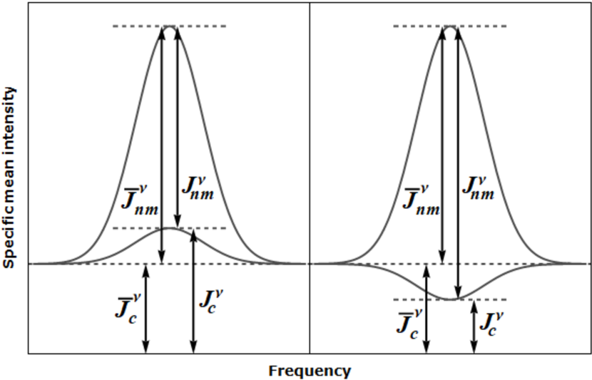
Figure 4: The effects of optical depths on the line and continuum radiation within a spectral line. The left panel shows the situation for $\tau_{\nu}<-1$ and the right panel shows the situation for $\tau_{\nu}>1$

Fig. 5 illustrates the effect of the electron density on the emitted spectrum of H$n\alpha$ lines. The kinetic temperature is the same for all of the models shown ($T_{\mathrm{e}}=10^{4}$ K) and the path length is chosen to show a pronounced bump for each case. The H$n\alpha$ lines that exhibit masing are mostly determined by the electron density, with masing occurring at lower $n$-levels for higher densities. The behaviour of the the H$n\alpha$ lines in the optically thick regime (high $n$) is independent of density.

Figure 5: Emitted spectrum of H$n\alpha$ transitions for masing region at electron temperature $T_{\mathrm{e}}=10^{4}$ K for a range of electron densities.

The effects of temperature on the emitted spectrum of a hydrogen maser region is much less pronounced than that of electron density. The values of $n$ where maser action occurs increases slightly towards higher $n$-levels as the temperature increases.

6.3 Comparison with optically thin and $n$-model results

Departure coefficients calculated assuming optically thin conditions (C³ models) are often used as a first approximation when doing HRL maser calculations, see for example Strelnitski et al. (1996a) and Báez-Rubio et al. (2013). It has also been argued that due to the high densities at which HRL masers occur, it is reasonable to neglect the $l$-structure of the atoms and use the results of an $n$-model (Strelnitski et al., 1996a; Hengel & Kegel, 2000).

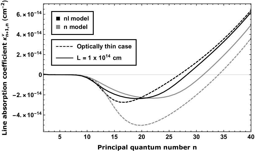
Figure 6: Absorption coefficients at line centre for H$n\alpha$ transition lines as calculated by different model assumptions as indicated in the legend. The electron temperature was set to $T_{\mathrm{e}}=10^{4}$ K and the electron density to $N_{\mathrm{e}}=10^{8}$ cm^-3.

Fig. 6 shows the line absorption coefficients at line centre of H$n\alpha$ as calculated using the level populations from models with different assumptions. Using the optically thin $n$-model results overestimates the maser gain by a factor of a few. Both the $n$-models (C³ and EPA) will overestimate the range of H$n\alpha$ transitions that can exhibit masing towards higher $n$-levels for a given set of conditions. The two $nl$-model results are similar, and deciding which to use will depend on the accuracy required for a specific application. The EPA $nl$-model predictions are more accurate than the C³ $nl$-model results in two ways, namely the $n$-level where the most maser gain will be seen and the range of lines over which maser action can occur.

Figure 7: Similar to Fig. 2, but using $b_{nl}$ values calculated in the optically thin approximation for all path lengths.

Fig. 7 shows the predicted line intensities if level populations from a C³ $nl$-model are used as opposed to those from the EPA $nl$-model that was illustrated in Fig. 2. In the C³ case, the maximum maser gain is shifted to a lower $n$-level and the bump feature is much sharper because the level populations have not been changed by the diffuse radiation. Using the C³ $n$-model results show a similar trend, but with the bump feature much exaggerated, as expected from the large magnitude of the line absorption coefficient shown in Fig. 6.

Strelnitski et al. (1996a) discuss the possibility of saturation in higher frequency lines “attracting” lower frequency lines to exhibit masing. Saturation in one of the masing lines, say $2\rightarrow 1$, will cause a decrease in the upper level of the transition, level $2$. This will increase the inversion between levels $3$ and $2$ and therefore the $3\rightarrow 2$ line will increase in intensity. If this process is effective enough, masing will start in the $3\rightarrow 2$ transition and the mechanism can diffuse out to even higher levels.

This behaviour is seen in the EPA model and is illustrated in Fig. 8, which shows how the total optical depths at certain H$n\alpha$ line frequencies changes as $L$ is increased. The optical depths at the H$27\alpha$ to H$30\alpha$ transition frequencies are positive for small values of $L$ and become negative and start to exhibit masing behaviour at some larger value of $L$. This occurs when the H$n\alpha$ transitions for lower $n$-levels’ degree of saturation have increased enough to increase the inversion of higher transitions, expanding the range of lines where maser action is possible.

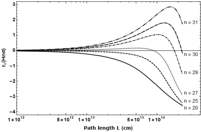
Figure 8: The change in optical depths with increasing path length for selected H$n\alpha$ transitions under conditions of $T_{\mathrm{e}}=10^{4}$ K and $N_{\mathrm{e}}=10^{8}$ cm^-3.

6.4 Comparison with observations

We compare results from the model with observations obtained by Thum et al. (1995) and Thum et al. (1998) for MWC 349A. This is the best studied hydrogen maser region at present and intensity data is available over a large range of frequencies. Aleman et al. (2018) more recently published observations of the nebula Mz 3 where hydrogen masing is also observed. The line intensity ratios of Aleman et al. (2018) are very similar to those of Thum et al. (1998), but the observations cover a much smaller frequency range than for MWC 349A. The limited observations do not show the complete bump structure in the H$n\alpha$ spectrum, so the model presented here cannot be used to constrain the physical parameters adequately.

The three sets of data that were used to find a reasonable model are the H$n\alpha$ fluxes from Thum et al. (1998), the $\beta/\alpha$ ratios for which the lines are close in $n$ from the same paper, and the $\beta/\alpha$ ratios for which the lines are close in frequency from Thum et al. (1995). An H$n\beta$ line represents the transition $n+2\rightarrow n$. The results from the EPA model that gave a reasonable fit considering all three sets of data occur for $T_{\mathrm{e}}=11\,000$ K, $N_{\mathrm{e}}=7\times 10^{7}$ cm^-3 and $L=2.7\times 10^{14}$ cm. These parameters are similar to the values obtained by Báez-Rubio et al. (2013) for the disc of MWC 349A which is the putative source of the maser emission. It is possible to get a model that matches one of the sets of data better than the chosen model, but it would be very inaccurate for the others. The aim of this fit is not to determine exact properties of MWC 349A, but to show that the EPA model gives results consistent with current observations.

Fig. 9 compares the data of Thum et al. (1998) and the chosen fit produced by the current model. The figure shows the observable integrated line intensities $\bar{J}_{n+1,n}$ obtained from equation (9) of H$n\alpha$ transitions relative to the H$10\alpha$ intensity. The model greatly underestimates the observable intensities for lines with $n>40$. It is believed that observed $\alpha$-lines with $n>38$ originate in the outflow and not in the disc where the masers are formed (Planesas et al., 1992). The conditions in the outflow are different to those in the disc.

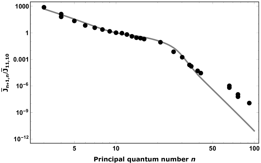
Figure 9: Results from the model (solid line) compared to data from Thum et al. (1998) (circles) for integrated line intensities of H$n\alpha$ transitions relative to H$10\alpha$. $T_{\mathrm{e}}=11\,000$ K, $N_{\mathrm{e}}=7\times 10^{7}$ cm^-3 and $L=2.7\times 10^{14}$ cm.

Fig. 10 shows the ratios of the integrated observed H$n\beta$ and H$n\alpha$ lines with the same upper level (black circles) for the model (solid line) shown in Fig. 9. Agreement between the observations and model is good, except for the lowest $n$ levels. Because the population of the ground level is set artificially to a fixed degree of ionization, the results for the lowest $n$ levels are not reliably determined by the model. The figure also shows the model predictions for the ratio for $n>16$. The results for $n>40$ will probably not be observed, since the measured lines from MWC 349A at those frequencies are not emitted from the disc. A list of H$n\alpha$, H$n\beta$ and H$n\gamma$ lines that occur within the frequency bands of ALMA is given in Table 2.

Figure 10: The ratio of H$n\alpha$ and H$n\beta$ lines with the same upper level. Circles show observations from Thum et al. (1998), the solid line shows results from the same model as in Fig. 9.

A comparison between our model results for $T_{\mathrm{e}}=11\,000$ K, $N_{\mathrm{e}}=7\times 10^{7}$ cm^-3 and $L=2.7\times 10^{14}$ cm. and the observations of Thum et al. (1995) for $\beta/\alpha$ ratios that are close in frequency is presented in Table 1. Most ratios could be fitted within the given ranges of Thum et al. (1995). The worst outlier is the ratio 48$\beta$/40$\alpha$, which is consistent with the model’s inability to fit lines with $n>40$.

Table 1: Model results compared to observed ratios of H$n\beta$/H$n\alpha$ pairs that are close in frequency as published by Thum et al. (1995).

Lines	Model ratio (%)	Observed ratio (%)
37$\beta$/30$\alpha$	9.9	$<12$
33$\beta$/26$\alpha$	4.2	$<10$
39$\beta$/31$\alpha$	9.3	$12\pm 3$
33$\beta$/26$\alpha$	4.2	$8.5\pm 1.5$
32$\beta$/26$\alpha$	5.6	$4.5\pm 1.5$
45$\beta$/36$\alpha$	15	$<18$
38$\beta$/30$\alpha$	7.1	$6.6\pm 1.5$
48$\beta$/40$\alpha$	31	$14\pm 2$

6.5 Ratios of $\alpha$- and $\beta$-lines

Comparing the intensities of H$n\beta$ lines to those of H$n\alpha$ transitions can provide additional information regarding the physical conditions in the emitting region. Strelnitski et al. (1996b) concluded that it is preferable to consider $\beta/\alpha$ pairs that are close in $n$-value for masing regions, as opposed to pairs that are close in frequency. This section reviews some general theoretical trends that should be observable in masing regions.

Figure 11: The ratio of the observable line centre $\bar{J}^{\nu}_{n+1,n-1}$ to continuum intensities of H$(n-1)\beta$ lines for a gas with $T_{\mathrm{e}}=10^{4}$ K and $N_{\mathrm{e}}=10^{8}$ cm^-3 for various path lengths.

Fig. 11 is a plot of the ratio of the line intensity $\bar{J}^{\nu}_{n+1,n-1}$ and continuum vs $n$ which gives an indication of the observability of H$(n-1)\beta$ transitions (i.e. $n+1\rightarrow n-1$) for a masing gas. The solid line in the graph is an approximation of the optically thin case. For larger optical depths, the $\beta$-lines are slightly enhanced in the same $n$-region as the $\alpha$-lines, but they are not technically masing. As the path length is increased for the higher $n$-transitions, the observable line to continuum ratio decreases.

Figure 12: The model ratios of $\beta$- and $\alpha$-lines with the same upper level for a masing gas with $T_{\mathrm{e}}=10^{4}$ K and $N_{\mathrm{e}}=10^{8}$ cm^-3 for various path lengths. The inset magnifies the behaviour at small $n$.

For a single emitting atom, the intensity of the $\alpha$-lines will always be greater than or equal to the intensity of the $\beta$-lines, because the $\alpha$-transitions have a larger transition probability than the $\beta$-transitions. But when considering a cloud, the difference in optical depths of the two transitions plays a role. The optical depths of the $\alpha$-transitions are much larger than those of the $\beta$-transitions for the same upper level, so that the $\alpha$-lines will always have a higher optical depth than their $\beta$ counterparts in the region where masing is not present.

Fig. 12 shows the behaviour of the observable integrated intensities $\bar{J}_{n+1,n-1}/\bar{J}_{n+1,n}$ as a function of $n$ for the case $T_{\mathrm{e}}=10^{4}$ K and $N_{\mathrm{e}}=10^{8}$ cm^-3 for different values of $L$ as produced by the EPA model. In the region where the H$n\alpha$ lines exhibit masing (inset in Fig. 12), the ratio is decreased as $L$ increases and the $\alpha$-lines outshine the non-masing $\beta$-lines. At high values of $n$ the situation is reversed with the $\beta$-lines becoming more intense than the $\alpha$-lines.

For example, for the $L=10^{14}$ cm case shown in Fig. 12 the line optical depths at line centre are $\tau_{41,40}=6$ and $\tau_{41,39}=0.8$. This means that the characteristic path length of a $\beta$-photon is larger than that of an $\alpha$-photon by a factor of about $7.5$ and we are observing $\beta$-photons coming from 7.5 times deeper in the cloud than the $\alpha$-photons. Therefore, the observed intensities of the $\beta$-lines are much brighter than those of the $\alpha$-lines if one or both of the transitions become optically thick. If both of the transitions are optically thick, the integrated intensity ratio of the two lines will tend to $\sim 5$, regardless of physical conditions.

The bump feature that emerges in Fig. 12 between the masing region and where both lines are optically thick is due to the interaction between the line and continuum opacities for the observable intensities. The maximum of the bump occurs at a point where $\tau_{\mathrm{c}}\approx 1.5$ for the $\beta$ lines.

7 Conclusions

Hydrogen recombination masers are a relatively new field of study with only a handful of examples detected so far. There are some important differences between molecular and atomic masers, both on the macro scale like the environments where they form, and at the atomic level like the pumping mechanism and interaction of many masing lines. The theoretical framework for these objects is still developing and the aim of this paper is to contribute to our understanding by constructing a theoretical model that specifically focuses on the atomic process rather than the geometry and kinematics.

The modeling of masers has some inherent complexities, since both the local level populations of the masing species and the non-local radiative transfer of the line photons have to be solved simultaneously in principle. Simplifying assumptions are often employed, for example the EPA used here. The EPA has limitations, but it is also a very useful tool to gain insight into overall emission from a cloud.

The effects of incorporating angular momentum changing collisions into an EPA model for hydrogen was shown. At the high electron densities where hydrogen masers form, the free-free emission from electrons will also effect the level populations of hydrogen.

A model for hydrogen recombination masers using the EPA have been constructed to evaluate the general behaviour of hydrogen emission from clouds with conditions where masing is possible. The observable effects of line of sight path length, electron temperature and electron density on the intensities of H$n\alpha$ emission lines have been investigated and discussed. The model results for varying path length corresponds well to our current understanding of how masers grow with increasing path length. The electron density has the biggest effect on which transitions will exhibit masing, whereas temperature has a larger effect on the behaviour of low frequency non-masing lines.

A fit of the model results was done to observations of the region MWC 349A where masing in hydrogen was first discovered. A good fit was obtained for a large range of frequencies with physical parameters in line with what other authors have obtained.

The behaviour of the ratios of H$n\alpha$ and H$n\beta$ lines that form from the same upper level have been examined. A fit was done to high frequency observations that are available and model predictions for lower frequency transitions are shown.

Appendix A Recombination lines observable with ALMA

Table 2: List of H$n\alpha$, H$n\beta$ and H$n\gamma$ lines that occur in the ALMA frequency bands.

Upper	Line	$\nu$	ALMA	Upper	Line	$\nu$	ALMA
level		($10^{11}$ Hz)	band	level		($10^{11}$ Hz)	band
20	H19$\alpha$	$8.880$	10	38	H35$\gamma$	$4.071$	8
22	H21$\alpha$	$6.624$	9	38	H36$\beta$	$2.600$	6
25	H24$\alpha$	$4.475$	8	39	H37$\beta$	$2.400$	6
26	H24$\beta$	$8.444$	10	40	H37$\gamma$	$3.468$	7
26	H25$\alpha$	$3.969$	8	40	H38$\beta$	$2.220$	6
27	H26$\alpha$	$3.536$	7	41	H38$\gamma$	$3.210$	7
28	H26$\beta$	$6.700$	9	41	H39$\beta$	$2.058$	5
28	H27$\alpha$	$3.164$	7	42	H39$\gamma$	$2.978$	7
29	H28$\alpha$	$2.843$	7	42	H40$\beta$	$1.911$	5
30	H27$\gamma$	$8.570$	10	43	H40$\gamma$	$2.767$	7
30	H29$\alpha$	$2.563$	6	43	H41$\beta$	$1.777$	5
31	H29$\beta$	$4.882$	8	44	H41$\gamma$	$2.576$	6
31	H30$\alpha$	$2.319$	6	44	H42$\beta$	$1.656$	5
32	H29$\gamma$	$6.987$	9	45	H42$\gamma$	$2.402$	6
32	H30$\beta$	$4.424$	8	45	H43$\beta$	$1.546$	4
32	H31$\alpha$	$2.105$	5	46	H43$\gamma$	$2.244$	6
33	H30$\gamma$	$6.341$	9	46	H44$\beta$	$1.445$	4
33	H31$\beta$	$4.022$	8	47	H44$\gamma$	$2.099$	5
33	H32$\alpha$	$1.917$	5	47	H45$\beta$	$1.352$	4
34	H32$\beta$	$3.667$	7	48	H45$\gamma$	$1.966$	5
34	H33$\alpha$	$1.750$	5	48	H46$\beta$	$1.268$	4
35	H33$\beta$	$3.352$	7	49	H46$\gamma$	$1.844$	5
35	H34$\alpha$	$1.602$	4	50	H47$\gamma$	$1.733$	5
35	H34$\alpha$	$1.602$	5	51	H48$\gamma$	$1.630$	4
36	H33$\gamma$	$4.823$	8	51	H48$\gamma$	$1.630$	5
36	H34$\beta$	$3.073$	7	52	H49$\gamma$	$1.535$	4
36	H35$\alpha$	$1.470$	4	53	H50$\gamma$	$1.447$	4
37	H34$\gamma$	$4.425$	8	54	H51$\gamma$	$1.366$	4
37	H35$\beta$	$2.823$	7	55	H52$\gamma$	$1.290$	4
37	H36$\alpha$	$1.353$	4

References

- Aleman et al. (2018) Aleman I., et al., 2018, MNRAS, 477, 4499
- Asensio Ramos & Elitzur (2018) Asensio Ramos A., Elitzur M., 2018, A&A, 616, A131
- Báez-Rubio et al. (2013) Báez-Rubio A., Martín-Pintado J., Thum C., Planesas P., 2013, A&A, 553, A45
- Báez-Rubio et al. (2018) Báez-Rubio A., Martín-Pintado J., Rico-Villas F., Jiménez-Serra I., 2018, ApJ, 867, L6
- Baker & Menzel (1938) Baker J. G., Menzel D. H., 1938, ApJ, 88, 52
- Brocklehurst & Salem (1977) Brocklehurst M., Salem M., 1977, Computer Physics Communications, 13, 39
- Chandra et al. (1984) Chandra S., Kegel W. H., Albrecht M. A., Varshalovich D. A., 1984, A&A, 140, 295
- Cox et al. (1995) Cox P., Martin-Pintado J., Bachiller R., Bronfman L., Cernicharo J., Nyman L.-A., Roelfsema P. R., 1995, A&A, 295, L39
- Cragg et al. (2002) Cragg D. M., Sobolev A. M., Godfrey P. D., 2002, MNRAS, 331, 521
- Dumont et al. (2003) Dumont A.-M., Collin S., Paletou F., Coupé S., Godet O., Pelat D., 2003, A&A, 407, 13
- Elitzur (1990) Elitzur M., 1990, ApJ, 363, 638
- Elitzur (1992) Elitzur M., ed. 1992, Astronomical masers Astrophysics and Space Science Library Vol. 170, doi:10.1007/978-94-011-2394-5.
- Elitzur (1994) Elitzur M., 1994, ApJ, 422, 751
- Elitzur & Asensio Ramos (2006) Elitzur M., Asensio Ramos A., 2006, MNRAS, 365, 779
- Ferland et al. (2013) Ferland G. J., et al., 2013, RMxAA, 49, 137
- Goldberg (1966) Goldberg L., 1966, ApJ, 144, 1225
- Gordon (1994) Gordon M. A., 1994, ApJ, 421, 314
- Gordon et al. (2001) Gordon M. A., Holder B. P., Jisonna Jr. L. J., Jorgenson R. A., Strelnitski V. S., 2001, ApJ, 559, 402
- Gray et al. (2018) Gray M. D., Mason L., Etoka S., 2018, MNRAS, 477, 2628
- Gray et al. (2019) Gray M. D., Baggott J., Westlake J., Etoka S., 2019, MNRAS, 486, 4216
- Hengel & Kegel (2000) Hengel C., Kegel W. H., 2000, A&A, 361, 1169
- Humphreys et al. (2001) Humphreys E. M. L., Yates J. A., Gray M. D., Field D., Bowen G. H., 2001, A&A, 379, 501
- Jiménez-Serra et al. (2011) Jiménez-Serra I., Martín-Pintado J., Báez-Rubio A., Patel N., Thum C., 2011, ApJ, 732, L27
- Jiménez-Serra et al. (2013) Jiménez-Serra I., Báez-Rubio A., Rivilla V. M., Martín-Pintado J., Zhang Q., Dierickx M., Patel N., 2013, ApJ, 764, L4
- Kallman & Bautista (2001) Kallman T., Bautista M., 2001, ApJS, 133, 221
- Kegel (1979) Kegel W. H., 1979, A&AS, 38, 131
- Koeppen & Kegel (1980) Koeppen J., Kegel W. H., 1980, A&AS, 42, 59
- Krolik & McKee (1978) Krolik J. H., McKee C. F., 1978, ApJS, 37, 459
- Langer & Watson (1984) Langer S. H., Watson W. D., 1984, ApJ, 284, 751
- Lockett & Elitzur (1992) Lockett P., Elitzur M., 1992, ApJ, 399, 704
- Martín-Pintado (2002) Martín-Pintado J., 2002, in Migenes V., Reid M. J., eds, IAU Symposium Vol. 206, Cosmic Masers: From Proto-Stars to Black Holes. p. 226
- Martin-Pintado et al. (1989a) Martin-Pintado J., Bachiller R., Thum C., Walmsley M., 1989a, A&A, 215, L13
- Martin-Pintado et al. (1989b) Martin-Pintado J., Thum C., Bachiller R., 1989b, A&A, 222, L9
- Martin-Pintado et al. (1994) Martin-Pintado J., Neri R., Thum C., Planesas P., Bachiller R., 1994, A&A, 286, 890
- Murchikova et al. (2019) Murchikova E. M., Phinney E. S., Pancoast A., Blandford R. D., 2019, Nature, 570, 83
- Nesterenok (2016) Nesterenok A. V., 2016, MNRAS, 455, 3978
- Oster (1961) Oster L., 1961, Rev. Mod. Phys., 33, 525
- Osterbrock (1962) Osterbrock D. E., 1962, ApJ, 135, 195
- Planesas et al. (1992) Planesas P., Martin-Pintado J., Serabyn E., 1992, ApJ, 386, L23
- Ponomarev (1994) Ponomarev V. O., 1994, Astronomy Letters, 20, 151
- Ponomarev et al. (1994) Ponomarev V. O., Smith H. A., Strelnitski V. S., 1994, ApJ, 424, 976
- Prozesky & Smits (2018) Prozesky A., Smits D. P., 2018, MNRAS, 478, 2766
- Röllig et al. (1999) Röllig M., Kegel W. H., Mauersberger R., Doerr C., 1999, A&A, 343, 939
- Rule et al. (2013) Rule E., Loeb A., Strelnitski V. S., 2013, ApJ, 775, L17
- Rybicki & Hummer (1991) Rybicki G. B., Hummer D. G., 1991, A&A, 245, 171
- Sánchez Contreras et al. (2017) Sánchez Contreras C., Báez-Rubio A., Alcolea J., Bujarrabal V., Martín-Pintado J., 2017, A&A, 603, A67
- Sobolev et al. (1997) Sobolev A. M., Cragg D. M., Godfrey P. D., 1997, A&A, 324, 211
- Spaans & Norman (1997) Spaans M., Norman C. A., 1997, ApJ, 488, 27
- Storey & Hummer (1995) Storey P. J., Hummer D. G., 1995, MNRAS, 272, 41