Dirac neutrino from the breaking of Peccei-Quinn symmetry

Abstract

We propose a model where Dirac neutrino mass is obtained from small vacuum expectation value (VEV) of neutrino-specific Higgs doublet without fine-tuning problem. The small VEV results from a seesaw-like formula with the high energy scale identified as the Peccei-Quinn (PQ) symmetry breaking scale. Axion can be introduced à la KSVZ or DFSZ. The model suggests neutrino mass, solution to the strong CP problem, and dark matter may be mutually interconnected.

I Introduction

Neutrino mass, strong CP problem, and the existence of dark matter are some hints that call for new physics (NP) beyond the standard model (SM). In this paper we consider a new physics (NP) model which can address these three problems simultaneously without fine-tuning.

Neutrino mass can be generated in neutrino-specific two Higgs doublet model ($\nu$THDM) where one Higgs doublet $\Phi_{1}$ with VEV $v_{1}(\sim 1\,{\rm eV})$ couples only to lepton doublet and right-handed neutrinos and the other Higgs doublet $\Phi_{2}$ with VEV $v_{2}(=246\,{\rm GeV})$ couples to all the other quarks and charged-leptons Ma (2001); Grimus et al. (2009); Wang et al. (2006); Davidson and Logan (2009); Ma and Popov (2017); Baek and Nomura (2017). We assume a global $U(1)_{X}$ symmetry under which $\nu_{R}$ and $\Phi_{1}$ are charged. The symmetry prohibits the mass term for the right-handed neutrinos. Therefore the neutrino gets only Dirac mass term and its Yukawa coupling can be of order one. The tiny VEV $v_{1}$ necessary to explain neutrino mass can be generated by seesaw-like relation in which the high-energy scale is the electroweak scale Davidson and Logan (2009); Ma and Popov (2017); Baek and Nomura (2017). The scalar $S$ which is a SM-singlet but charged under $U(1)_{X}$ breaks the global symmetry spontaneously, and can couple to an electroweak-scale WIMP dark matter which is stabilized by a remnant discrete symmetry Ma and Popov (2017); Baek and Nomura (2017); Baek et al. (2018).

In this paper we consider a scenario in which the VEV $v_{S}$ of $S$ and the mass scale of $\Phi_{1}$ is lifted to a very large scale $\sim 10^{12}$ GeV. The neutrino mass is generated by a mechanism shown in Figure 1. The diagram generates a VEV $v_{1}$, which can be written as

$$v_{1}\approx{\sqrt{2}\mu v_{2}v_{S}\over m_{11}^{2}},$$ (1)

where $v_{2}=246$ GeV, $v_{S}\sim m_{11}\sim{\cal O}(10^{12})$ GeV, $m_{11}$ being the mass scale of $\Phi_{1}$. We extend the model to incorporate axions so as to solve the strong CP problem and dark matter candidate. In this case the $U(1)_{X}$ is identified with the Peccei-Quinn (PQ) symmetry $U(1)_{\rm PQ}$, and after $S$ getting VEV the Nambu-Goldstone boson becomes an axion. Therefore the neutrino mass and the axion are connected by the scalar $S$. Since $m_{11}\sim{\cal O}(10^{12})$ GeV, the low energy constraints such as collider searches and charged lepton number violating processes are irrelevant. Since the axion is also a good cold dark matter candidate, the scenario also solves the dark matter problem with the axion as a cold dark matter. Symmetry arguments show that the hierarchy $v_{1}(\sim{\cal O}(1\,{\rm eV}))\ll v_{2}(\simeq 246\,{\rm GeV})\ll v_{S}(\sim{\cal O}(10^{12}\,{\rm GeV}))$ is technically natural.

The $\nu$THDM on its own does not provide an axion candidate. We make the Nambu-Goldstone boson coming from the spontaneous breaking of the $U(1)_{X}$ in the model of Baek and Nomura (2017) an axion by introducing either heavy vector-like quarks $\Psi_{L,R}$ (KSVZ-type axion) or additional Higgs doublet (DFSZ-type axion). It turns out that the phenomenology of the axion in the model is very close to that of original KSVZ Kim (1979); Shifman et al. (1980) and DFSZ Dine et al. (1981); Zhitnitsky (1980) axion models, respectively. There are many attempts to connect axion and neutrino mass in the literature Berezhiani and Khlopov (1991); Gu and He (2006); Chen and Tsai (2013); Dasgupta et al. (2014); Ma (2015); Bertolini et al. (2015); Ahn and Chun (2016); Gu (2016); Ma et al. (2018); Suematsu (2018); Ahn (2018); Reig and Srivastava (2019); Carvajal and Zapata (2019).

The paper is organized as follows. In Section II, we briefly review the $U(1)_{X}$ model studied in Baek and Nomura (2017) with $v_{S}$ lifted to PQ breaking scale and show that the large hierarchy among the disparate scales is technically natural. In Section III, the model is extended so that the KSVZ-type or the DFSZ-type axion is introduced. The phenomenology of the axion is outlined. In Section IV, we conclude the paper.

II The model

We briefly recapitulate the model considered in Baek and Nomura (2017) before discussing the VEVs and their naturalness. Since we promote $U(1)_{X}$ of Baek and Nomura (2017); Baek et al. (2018) to $U(1)_{\rm PQ}$ in Section III, we will call the global symmetry $U(1)_{\rm PQ}$ from now on. The charge assignment under the SM and $U(1)_{\rm PQ}$ is shown in Table 1. The left-handed SM fermion fields, which are not listed in Table 1, are assigned with PQ-charge 0.

	Scalar Fields			Fermions				KSVZ		DFSZ
	$\Phi_{1}$	$\Phi_{2}$	$S$	$u_{Ri}$	$d_{Ri}$	$e_{Ri}$	$\nu_{Ri}$	$\Psi_{L}$	$\Psi_{R}$	$\Phi_{d}$	$\Phi_{u}$
$SU(3)_{C}$	$\bm{1}$	$\bm{1}$	$\bm{1}$	$\bm{3}$	$\bm{3}$	$\bm{1}$	$\bm{1}$	$\bm{3}$	$\bm{3}$	$\bm{1}$	$\bm{1}$
$SU(2)_{L}$	$\bm{2}$	$\bm{2}$	$\bm{1}$	$\bm{1}$	$\bm{1}$	$\bm{1}$	$\bm{1}$	$\bm{1}$	$\bm{1}$	$\bm{2}$	$\bm{2}$
$U(1)_{Y}$	$\frac{1}{2}$	$\frac{1}{2}$	$0$	${2\over 3}$	$-{1\over 3}$	$-1$	$0$	$e_{\Psi}$	$e_{\Psi}$	$\frac{1}{2}$	$\frac{1}{2}$
${U(1)_{\rm PQ}}$	$Z_{1}(X_{1})$	$Z_{2}(X_{2})$	$Z_{S}(X_{S})$	$Z_{u_{R}}(X_{u_{R}})$	$Z_{d_{R}}(X_{d_{R}})$	$Z_{e_{R}}(X_{e_{R}})$	$Z_{\nu_{R}}(X_{\nu_{R}})$	$0$	$Z_{\Psi_{R}}(X_{\Psi_{R}})$	$Z_{d}(X_{d})$	$Z_{u}(X_{u})$

Table 1: Charge assignment under the SM and $U(1)_{\rm PQ}$. For the $U(1)_{\rm PQ}$, the $Z$’s ($X$’s) are (effective) PQ charges. The $Z$’s are independent of VEVs, while $X$’s may depend on VEVs. The explicit values for $Z$’s and $X$’s depend on the models and will be shown for each model later. KSVZ (DFSZ) corresponds to the model extension for the KSVZ-(DFSZ-) type axion. We normalize $Z_{S}=X_{S}=1$ throughout the paper. We assign $Z_{\Psi_{R}}=-1$, $Z_{d}=-1$, and $Z_{u}=1$.

The Yukawa interactions consistent with the SM gauge symmetry and the $U(1)_{\rm PQ}$ symmetry are written as

$${\cal L} =-y^{u}_{ij}\overline{Q}_{Li}\widetilde{\Phi}_{2}u_{Rj}-y^{d}_{ij}\overline{Q}_{Li}\Phi_{2}d_{Rj}-y^{e}_{ij}\overline{L}_{Li}\Phi_{2}e_{Rj}-y^{\nu}_{ij}\overline{L}_{Li}\widetilde{\Phi}_{1}\nu_{Rj}+h.c.,$$ (2)

where $i,j=1,2,3$ are generation indices, and $\widetilde{\Phi}_{1(2)}=i\sigma^{2}\Phi^{*}_{1(2)}$. The scalar potential is given in the form

$$V =+m_{11}^{2}\Phi_{1}^{\dagger}\Phi_{1}-m_{22}^{2}\Phi_{2}^{\dagger}\Phi_{2}-m_{SS}^{2}S^{\dagger}S-(\mu\Phi_{1}^{\dagger}\Phi_{2}S+h.c)$$

$$+\lambda_{1}(\Phi_{1}^{\dagger}\Phi_{1})^{2}+\lambda_{2}(\Phi_{2}^{\dagger}\Phi_{2})^{2}+\lambda_{3}(\Phi_{1}^{\dagger}\Phi_{1})(\Phi_{2}^{\dagger}\Phi_{2})+\lambda_{4}(\Phi_{1}^{\dagger}\Phi_{2})(\Phi_{2}^{\dagger}\Phi_{1})$$

$$+\lambda_{S}(S^{\dagger}S)^{2}+\lambda_{1S}(\Phi_{1}^{\dagger}\Phi_{1})(S^{\dagger}S)+\lambda_{2S}(\Phi_{2}^{\dagger}\Phi_{2})(S^{\dagger}S).$$ (3)

Note that the sign in front of $m_{11}^{2}$ is “+”. We assume $m_{11}^{2}>0$, $m_{22}^{2}>0$, and $m_{SS}^{2}>0$. We can also take $\mu$ to be positive without loss of generality because any complex phase can be absorbed by the redefinition of $S$. We can decompose the scalars as

$$\Phi_{1}=\begin{pmatrix}\phi_{1}^{+}\\ {1\over\sqrt{2}}(v_{1}+h_{1}+ia_{1})\end{pmatrix},\quad\Phi_{2}=\begin{pmatrix}\phi_{2}^{+}\\ {1\over\sqrt{2}}(v_{2}+h_{2}+ia_{2})\end{pmatrix},\quad S={1\over\sqrt{2}}(v_{S}+h_{S}+ia_{S}).$$ (4)

For the vacuum stability we impose the copositivity condition Kannike (2012):

$$\lambda_{1}>0,\quad\lambda_{2}>0,\quad\lambda_{S}>0,$$

$$\tilde{\lambda}_{12}\equiv{1\over 2}(\lambda_{3}+\lambda_{4})+\sqrt{\lambda_{1}\lambda_{2}}>0,$$

$$\tilde{\lambda}_{1S}\equiv\frac{1}{2}\lambda_{1S}+\sqrt{\lambda_{1}\lambda_{S}}>0,$$

$$\tilde{\lambda}_{2S}\equiv\frac{1}{2}\lambda_{2S}+\sqrt{\lambda_{2}\lambda_{S}}>0,$$

$$\sqrt{\lambda_{1}\lambda_{2}\lambda_{3}}+\frac{1}{2}(\lambda_{3}+\lambda_{4})\sqrt{\lambda_{S}}+\frac{1}{2}\lambda_{1S}\sqrt{\lambda_{2}}+\frac{1}{2}\lambda_{2S}\sqrt{\lambda_{1}}+\sqrt{2\tilde{\lambda}_{12}\tilde{\lambda}_{1S}\tilde{\lambda}_{2S}}>0.$$ (5)

The conditions in (5) are automatically satisfied when all the $\lambda$’s are positive, which we assume in this paper. The minimization conditions for the potential along the direction of neutral fields $h_{1},h_{2}$, and $h_{S}$ are

$$+2m_{11}^{2}v_{1}+2\lambda_{1}v_{1}^{3}+v_{1}(\lambda_{1S}v_{S}^{2}+\lambda_{3}v_{2}^{2}+\lambda_{4}v_{2}^{2})-\sqrt{2}\mu v_{2}v_{S}=0,$$ (6)

$$-2m_{22}^{2}v_{2}+2\lambda_{2}v_{2}^{3}+v_{2}(\lambda_{2S}v_{S}^{2}+\lambda_{3}v_{1}^{2}+\lambda_{4}v_{1}^{2})-\sqrt{2}\mu v_{1}v_{S}=0,$$ (7)

$$-2m_{SS}^{2}v_{S}+2\lambda_{S}v_{S}^{3}+v_{S}(\lambda_{1S}v_{1}^{2}+\lambda_{2S}v_{2}^{2})-\sqrt{2}\mu v_{1}v_{2}=0.$$ (8)

From the above coupled equations we solve for VEVs: $v_{S}$, $v_{2}$, and $v_{1}$. The solution consistent with our assumption, $v_{S}\gg v_{2}\gg v_{1}$, is given approximately by

$$v_{S} \approx{m_{SS}\over\sqrt{\lambda_{S}}},$$

$$v_{2} \approx\sqrt{2m_{22}^{2}-\lambda_{2S}v_{S}^{2}\over 2\lambda_{2}}.$$ (9)

To ensure small $v_{1}$, we make an additional assumption,

$$\lambda_{1S}v_{S}^{2}+(\lambda_{3}+\lambda_{4})v_{2}^{2}+2m_{11}^{2}>0,$$ (10)

which can be easily satisfied since $m_{11}^{2}\sim{\cal O}(10^{12}\,{\rm GeV})^{2}$ dominates the left hand side of the inequality. If $\mu=0$, the only solution for (6) is $v_{1}=0$. For $\mu\neq 0$, the solution is proportional to $\mu$ and is obtained in a good approximation to be

$$v_{1} \approx{\sqrt{2}\mu v_{2}v_{S}\over\lambda_{1S}v_{S}^{2}+(\lambda_{3}+\lambda_{4})v_{2}^{2}+2m_{11}^{2}}\approx{\sqrt{2}\mu v_{2}v_{S}\over 2m_{11}^{2}},$$ (11)

where the last relation follows because $m_{11}^{2}\gg|\lambda_{1S}|v_{S}^{2}\gg|\lambda_{3}+\lambda_{4}|v_{2}^{2}$. As we mentioned in Section I, we require $v_{1}\sim{\cal O}(1\,{\rm eV})$ to explain small neutrino mass. We can easily achieve this by taking, for example, $\mu\sim 1\,{\rm GeV}$, when $m_{11}\sim v_{S}\sim 10^{12}\,{\rm GeV}$. The Feynman diagram for the neutrino mass is shown in Figure 1. The red (black) arrows represent the flow of $U(1)_{\rm PQ}$ (lepton number) current. We can see the neutrino mass is effectively given by

$$m_{\nu_{ij}}\sim y^{\nu}_{ij}\frac{\mu v_{2}v_{S}}{m_{11}^{2}},$$ (12)

from which we can check $v_{1}$ is the form in (11).

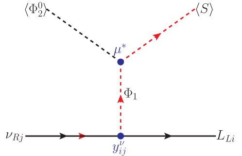
Figure 1: Feynman diagram for the neutrino mass generation. The red (black) arrows represent the flow of $U(1)_{\rm PQ}$ (lepton number) current.

The superheavy $\Phi_{1}$ makes the model escape the collider and other low energy bound easily. It is noted that $\Phi_{1}$ is superheavy but its VEV is tiny. The bottomline is that the main contribution to the masses of $\Phi_{1}$ components come from the bare mass term $m_{11}^{2}$, which makes them superheavy, while $v_{1}$ generated by the diagram shown in Figure 1 can remain tiny. The small $\mu$ which makes $v_{1}$ tiny is technically natural because the symmetry of the Lagrangian (3) is enhanced in the $\mu\to 0$ limit Baek and Nomura (2017). This can be seen also from the RG equation for $\mu$,

$${d\mu(Q)\over d\log Q} ={1\over 8\pi^{2}}\mu\left(\lambda_{1S}+\lambda_{2S}+\lambda_{3}+2\lambda_{4}\right),$$ (13)

which shows that $\mu=0$ is a fixed point, making small $\mu$ remain small under the change of scale.

We also need to address the large hierarchy between the electroweak scale and the PQ-breaking scale. The large hierarchy may cause naturalness problem by generating quadratic divergence in the quantum corrections of Higgs mass. A solution to this problem comes from Poincaré protection Foot et al. (2014). We adopt their paradigm by taking

$$\lambda_{2S}\lesssim{\cal O}\left(m_{H}^{2}\over m_{S}^{2}\right)\sim 10^{-20}\left(m_{H}\over 100\,{\rm GeV}\right)^{2}\left(10^{12}\,{\rm GeV}\over m_{S}\right)^{2}.$$ (14)

We also take $\lambda_{1S}$ with similar size. Sending $(\lambda_{1S},\lambda_{2S})\to(0,0)$, the Poincaré symmetry is enhanced, making the small $(\lambda_{1S},\lambda_{2S})$ technically natural Foot et al. (2014). We can also check this from the renormalization group running of $\lambda_{1S}$ and $\lambda_{2S}$, which is given by,

$${d\lambda_{1S}(Q)\over d\log Q} ={1\over 8\pi^{2}}\Bigg{[}2\lambda_{1S}(\lambda_{1S}+3\lambda_{1}+2\lambda_{S})+\lambda_{2S}(2\lambda_{3}+\lambda_{4})\Bigg{]},$$

$${d\lambda_{2S}(Q)\over d\log Q} ={1\over 8\pi^{2}}\Bigg{[}2\lambda_{2S}(\lambda_{2S}+3\lambda_{2}+2\lambda_{S})+\lambda_{1S}(2\lambda_{3}+\lambda_{4})\Bigg{]},$$ (15)

which reveals $(\lambda_{1S},\lambda_{2S})=(0,0)$ is a fixed point.

III Axions

Since the VEV $v_{S}$ can be naturally ${\cal O}(10^{12})$ GeV, we may identify this scale as the breaking scale of the PQ symmetry. By promoting the $U(1)_{X}$ symmetry to PQ symmetry $U(1)_{\rm PQ}$, we can introduce axion to solve the strong CP problem. From the charge assignments in Table 2, the axion field can be defined as Srednicki (1985)

$$a_{\rm PQ} ={1\over v^{0}_{\rm PQ}}\sum_{i=1,2,S}Z_{i}v_{i}a_{i}$$

$$={1\over v^{0}_{\rm PQ}}\Big{(}{1\over 2}v_{1}a_{1}-{1\over 2}v_{2}a_{2}+v_{S}a_{S}\Big{)},$$ (16)

where $v^{0}_{\rm PQ}=(\sum_{i}(Z_{i}v_{i})^{2})^{1/2}=(v_{1}^{2}/4+v_{2}^{2}/4+v_{S}^{2})^{1/2}$. However, $a_{\rm PQ}$ is not orthogonal to the Nambu-Goldstone boson, $a_{Z}=(v_{1}a_{1}+v_{2}a_{2})/(v_{1}^{2}+v_{2}^{2})^{1/2}$, which is eaten by the longitudinal component of $Z$ boson. The physical axion field is obtained by orthogonalization:

$$a =a_{\rm PQ}-\frac{v_{1}^{2}-v_{2}^{2}}{2v^{0}_{\rm PQ}(v_{1}^{2}+v_{2}^{2})^{1/2}}a_{Z}$$

$$=\frac{1}{v^{0}_{\rm PQ}(v_{1}^{2}+v_{2}^{2})}(v_{1}v_{2}^{2}a_{1}-v_{1}^{2}v_{2}a_{2}+(v_{1}^{2}+v_{2}^{2})v_{S}a_{S}).$$ (17)

We note that $v^{0}_{\rm PQ}$ should be changed to $v_{\rm PQ}\equiv(v_{S}^{2}+v_{1}^{2}v_{2}^{2}/(v_{1}^{2}+v_{2}^{2}))^{1/2}$ for $a$ to be canonically normalized. Now we can define the effective PQ charges, $X_{i}$ ($i=1,2,S$), so that

$$a=\frac{1}{v_{\rm PQ}}\sum_{i=1,2,S}X_{i}v_{i}a_{i}.$$ (18)

Then we get

$$X_{1}=\frac{v_{2}^{2}}{v_{1}^{2}+v_{2}^{2}},\quad X_{2}=-\frac{v_{1}^{2}}{v_{1}^{2}+v_{2}^{2}},\quad X_{S}=1.$$ (19)

Equivalently, we can parametrize the Higgs fields in terms of the physical axion $a$ as

$$\Phi_{1}={v_{1}\over\sqrt{2}}e^{iaX_{1}/v_{\rm PQ}}\begin{pmatrix}0\\ 1\end{pmatrix},\quad\Phi_{2}={v_{2}\over\sqrt{2}}e^{iaX_{2}/v_{\rm PQ}}\begin{pmatrix}0\\ 1\end{pmatrix},\quad S={v_{S}\over\sqrt{2}}e^{iaX_{S}/v_{\rm PQ}},$$ (20)

where $X_{1},X_{2}$, and $X_{S}$ are their effective PQ charges. We will calculate the $X$’s again and show that they agree with (19). We take the normalization $X_{S}\equiv 1$. The $\mu$ term in (3) dictates

$$-X_{1}+X_{2}+X_{S}=0.$$ (21)

Since $a$ should not mix with the $Z$-boson, we get a condition

$$X_{1}v_{1}^{2}+X_{2}v_{2}^{2}=0.$$ (22)

We refer the reader to Appendix A for details of the above relation. Then we get

$$X_{1}={v_{2}^{2}\over v_{1}^{2}+v_{2}^{2}},\quad X_{2}=-{v_{1}^{2}\over v_{1}^{2}+v_{2}^{2}}.$$ (23)

The SM electroweak vacuum is obtained to be $v_{\rm ew}\equiv\sqrt{v_{1}^{2}+v_{2}^{2}}\simeq 246$ GeV. The result with the normalization $X_{S}=1$ agrees with (19). Expanding (20) up to linear order, we can identify the axion field $a$ in terms of $(a_{1},a_{2},a_{S})$,

$$a ={1\over v_{\rm PQ}}(X_{1}v_{1}a_{1}+X_{2}v_{2}a_{2}+X_{S}v_{S}a_{S})$$

$$={1\over v_{\rm PQ}(v_{1}^{2}+v_{2}^{2})}(v_{1}v_{2}^{2}a_{1}-v_{1}^{2}v_{2}a_{2}+v_{\rm ew}^{2}v_{S}a_{S}){,}$$ (24)

which agrees with (17) up to the overall constant. From normalization condition we can express $v_{\rm PQ}$ as

$$v_{\rm PQ}=\left((X_{1}v_{1})^{2}+(X_{2}v_{2})^{2}+(X_{S}v_{S})^{2}\right)^{1/2}={1\over v_{1}^{2}+v_{2}^{2}}\left((v_{1}v_{2}^{2})^{2}+(v_{1}^{2}v_{2})^{2}+(v_{\rm ew}^{2}v_{S})^{2}\right)^{1/2}{,}$$ (25)

which is exactly what we obtained below (18). From (2) the effective charges for the other fields read

$$X_{u_{R}}=X_{2}={-{v_{1}^{2}\over v_{1}^{2}+v_{2}^{2}}},\quad X_{d_{R}}=X_{e_{R}}=-X_{2}={{v_{1}^{2}\over v_{1}^{2}+v_{2}^{2}}},\quad X_{\nu_{R}}=X_{1}={{v_{2}^{2}\over v_{1}^{2}+v_{2}^{2}}}.$$ (26)

	Scalar Fields			Fermions
	$\Phi_{1}(X_{1})$	$\Phi_{2}(X_{2})$	$S(X_{S})$	$u_{Ri}(X_{u_{R}})$	$d_{Ri}(X_{d_{R}})$	$e_{Ri}(X_{e_{R}})$	$\nu_{Ri}(X_{\nu_{R}})$
$U(1)_{\rm PQ}$	${1\over 2}\left({v_{2}^{2}\over v_{1}^{2}+v_{2}^{2}}\right)$	$-{1\over 2}\left(-{v_{1}^{2}\over v_{1}^{2}+v_{2}^{2}}\right)$	1 (1)	$-{1\over 2}\left(-{v_{1}^{2}\over v_{1}^{2}+v_{2}^{2}}\right)$	${1\over 2}\left({v_{1}^{2}\over v_{1}^{2}+v_{2}^{2}}\right)$	${1\over 2}\left({v_{1}^{2}\over v_{1}^{2}+v_{2}^{2}}\right)$	${1\over 2}\left({v_{2}^{2}\over v_{1}^{2}+v_{2}^{2}}\right)$

Table 2: The non-vanishing $U(1)_{\rm PQ}$ (effective) charges for the $\nu$THDM described by (2) and (3).

The non-vanishing PQ-charges for the $\nu$THDM described by (2) and (3) are summarized in Table 2. Since the PQ charges of $u_{Ri}$ and $d_{Ri}$ add to zero, the QCD anomaly cancels, and the Nambu-Goldstone boson $a$ cannot be QCD axion candidate in the model (2).

We can extend the model to make $a$ an axion to solve the strong CP problem in two ways. One method is to introduce a pair of heavy vector-like quarks $\Psi_{L,R}$ which couples to $S$ and weighs PQ-breaking scale, where $a$ becomes KSVZ-type axion Kim (1979); Shifman et al. (1980). The other one is by replacing $\Phi_{2}$ with a pair of Higgs doublet $\Phi_{u,d}$, where $\Phi_{u(d)}$ couples to $S$ and $u(d)$-type quarks, making $a$ DFSZ-type axion Dine et al. (1981); Zhitnitsky (1980). The charge assignments for the two possible scenarios are shown in Table 1 with tabs KSVZ and DFSZ. In both scenarios the seesaw-like relation (11) and axion decay constant in (28) and (46) share the PQ-breaking parameter $v_{S}$ in common, showing the interplay between neutrino mass and axion. As a consequence, neutrino experiments can constrain the parameter space of the axion model, and vice versa Peinado et al. (2019).

III.1 KSVZ-type axion

In the KSVZ-type scenario for axion we introduce heavy vector-like quarks in addition to fields shown in Table 2. We have Yukawa coupling for $\Psi$:

$$\Delta{\cal L}=-y_{\Psi}\overline{\Psi}_{L}S\Psi_{R}+h.c.$$ (27)

Then the (effective) PQ-charge of $\Psi_{R}$ is fixed: $Z_{\Psi_{R}}=-Z_{S}=-1$ ($X_{\Psi_{R}}=-X_{S}=-1$), assuming $Z_{\Psi_{L}}=0$ ($X_{\Psi_{L}}=0$). The Yukawa interactions and the scalar potential shown in (2) and (3) remain the same. As a consequence, the equations from (20) to (26) hold also in this model without any change. The PQ charges for this model are collected in Table 3

	Scalar Fields			Fermions				KSVZ
	$\Phi_{1}(X_{1})$	$\Phi_{2}(X_{2})$	$S(X_{S})$	$u_{Ri}(X_{u_{R}})$	$d_{Ri}(X_{d_{R}})$	$e_{Ri}(X_{e_{R}})$	$\nu_{Ri}(X_{\nu_{R}})$	$\Psi_{L}(X_{\Psi_{L}})$	$\Psi_{R}(X_{\Psi_{R}})$
$U(1)_{\rm PQ}$	${1\over 2}\left({v_{2}^{2}\over v_{1}^{2}+v_{2}^{2}}\right)$	$-{1\over 2}\left(-{v_{1}^{2}\over v_{1}^{2}+v_{2}^{2}}\right)$	1 (1)	$-{1\over 2}\left(-{v_{1}^{2}\over v_{1}^{2}+v_{2}^{2}}\right)$	${1\over 2}\left({v_{1}^{2}\over v_{1}^{2}+v_{2}^{2}}\right)$	${1\over 2}\left({v_{1}^{2}\over v_{1}^{2}+v_{2}^{2}}\right)$	${1\over 2}\left({v_{2}^{2}\over v_{1}^{2}+v_{2}^{2}}\right)$	$0(0)$	$-1(-1)$

Table 3: The $U(1)_{\rm PQ}$ (effective) charges for the KSVZ-type model described by (2), (3) and (27). The PQ charges for the fields not listed here all vanish.

Independently of the ratio $v_{1}/v_{2}$ the axion mass is given by Grilli di Cortona et al. (2016)

$$m_{a} ={f_{\pi}m_{\pi}\over{v_{\rm PQ}}}{\sqrt{m_{u}m_{d}}\over m_{u}+m_{d}}\simeq 5.7\,{\rm\mu eV}\left(10^{12}\,{\rm GeV}\over f_{a}\right),$$ (28)

where in the last equality we identified the axion decay constant $f_{a}\equiv v_{\rm PQ}$. The axion-photon coupling is

$${\cal L}_{a\gamma\gamma}=-\Big{[}6e_{\Psi}^{2}-\frac{2(4+z)}{3(1+z)}\Big{]}{a\over v_{\rm PQ}}\frac{e^{2}}{32\pi^{2}}F^{\mu\nu}\widetilde{F}_{\mu\nu}=\Big{[}6e_{\Psi}^{2}-1.92\Big{]}\frac{\alpha_{\rm em}}{2\pi f_{a}}\,a\,\bm{E}\cdot\bm{B}$$ (29)

The $a\gamma\gamma$-coupling is also independent of the ration $v_{1}/v_{2}$. The results (28) and (29) are in exact agreement with those of the original KSVZ model Kim (1979); Shifman et al. (1980). The difference comes in the couplings of the axion to electron and neutrinos. In general the axion coupling to fermions is written as Tanabashi et al. (2018),

$${\cal L}_{aff}=-\frac{C_{f}}{2f_{a}}\partial_{\mu}a\overline{f}\gamma^{\mu}\gamma_{5}f.$$ (30)

The tree level axion coupling to electrons (neutrinos) is $C_{e}=v_{1}^{2}/(v_{1}^{2}+v_{2}^{2})\;(C_{\nu}=v_{2}^{2}/(v_{1}^{2}+v_{2}^{2}))$, while they both vanish in the KSVZ model. However, the fact that $v_{1}\ll v_{2}$ makes the $C_{e}$ coupling practically indistinguishable from that in the KSVZ model. The axion coupling to neutrinos $C_{\nu}\approx 1$ and in principle can be probed through experiments such as neutrino oscillation Huang and Nath (2018).

III.2 DFSZ-type axion

We can also extend the Higgs sector to introduce a QCD axion Dine et al. (1981); Zhitnitsky (1980). We replace $\Phi_{2}$ with $\Phi_{u}$ and $\Phi_{d}$, where $\Phi_{u}$ couples only to the up-type quarks and $\Phi_{d}$ couples only to the down-type quarks. The charged-leptons can couple either to $\Phi_{d}$ (type-II) or to $\Phi_{u}$ (flipped). As in the original DFSZ model, we introduce

$$\Phi_{u}^{\dagger}\Phi_{d}S^{2}+h.c.$$ (31)

term to the Lagrangian. Now the $\mu$-term in (3) can take the form of either

$$-\mu\Phi_{1}^{\dagger}\Phi_{d}S+h.c.,$$ (32)

or

$$-\mu\Phi_{1}^{\dagger}\Phi_{u}S+h.c.,$$ (33)

but not both. The introduction of (31) and (32) (or (33)) does not spoil the smallness of $v_{1}$ in (11) and the naturalness arguments presented in Section II. The PQ charges are assigned as in Table 4. And the $X$’s are calculated as follows. The (31) gives a relation,

$$-X_{u}+X_{d}+2X_{S}=0,$$ (34)

where we will take the normalization $X_{S}=1$ as in the KSVZ scenario. From (32) ((33)) the effective PQ-charges should satisfy

$$-X_{1}+X_{d}+X_{S}=0,\quad(-X_{1}+X_{u}+X_{S}=0).$$ (35)

The axion does not mix with the SM $Z$-boson, if

$$X_{1}v_{1}^{2}+X_{d}v_{d}^{2}+X_{u}v_{u}^{2}=0,$$ (36)

where $\langle\Phi^{0}_{d(u)}\rangle=v_{d(u)}/\sqrt{2}$. Since $\sqrt{v_{u}^{2}+v_{d}^{2}+v_{1}^{2}}\equiv v_{\rm ew}\simeq 246$ GeV, $v_{d(u)}$ is at most at the electroweak scale. If the kinetic term of the axion is canonically normalized, we get

$$X_{1}^{2}v_{1}^{2}+X_{d}^{2}v_{d}^{2}+X_{u}^{2}v_{u}^{2}+X_{S}^{2}v_{S}^{2}=v_{\rm PQ}^{2}.$$ (37)

Now we can solve $X_{1}$, $X_{d}$ and $X_{u}$ from (34), (35), and (36), setting $X_{S}=1$: for (32) we get

$$X_{1} =\frac{v_{d}^{2}-v_{u}^{2}}{v_{1}^{2}+v_{d}^{2}+v_{u}^{2}},\quad X_{d}=-\frac{v_{1}^{2}+2v_{u}^{2}}{v_{1}^{2}+v_{d}^{2}+v_{u}^{2}},\quad X_{u}=\frac{v_{1}^{2}+2v_{d}^{2}}{v_{1}^{2}+v_{d}^{2}+v_{u}^{2}},$$ (38)

and for (33) we get

$$X_{1} =\frac{3v_{d}^{2}+v_{u}^{2}}{v_{1}^{2}+v_{d}^{2}+v_{u}^{2}},\quad X_{d}=-\frac{3v_{1}^{2}+2v_{u}^{2}}{v_{1}^{2}+v_{d}^{2}+v_{u}^{2}},\quad X_{u}=-\frac{v_{1}^{2}-2v_{d}^{2}}{v_{1}^{2}+v_{d}^{2}+v_{u}^{2}}.$$ (39)

Then the PQ-breaking scale $v_{\rm PQ}$ can be determined by (37). Inserting (38) and (39), we get

$$v_{\rm PQ}^{2}=v_{S}^{2}+\frac{v_{1}^{2}(v_{d}^{2}+v_{u}^{2})+4v_{d}^{2}v_{u}^{2}}{v_{1}^{2}+v_{d}^{2}+v_{u}^{2}},\;\text{and}\quad v_{\rm PQ}^{2}=v_{S}^{2}+\frac{v_{1}^{2}(9v_{d}^{2}+v_{u}^{2})+4v_{d}^{2}v_{u}^{2}}{v_{1}^{2}+v_{d}^{2}+v_{u}^{2}},$$ (40)

respectively. In this model the Yukawa interactions in (2) are written as

$${\cal L} =-y^{u}_{ij}\overline{Q}_{Li}\widetilde{\Phi}_{u}u_{Rj}-y^{d}_{ij}\overline{Q}_{Li}\Phi_{d}d_{Rj}-y^{e}_{ij}\overline{L}_{Li}\Phi_{q}e_{Rj}-y^{\nu}_{ij}\overline{L}_{Li}\widetilde{\Phi}_{1}\nu_{Rj}+h.c.,$$ (41)

where $q=d(u)$ for type-II (flipped) scenario for the lepton couplings to Higgs. From (41) we get

$$X_{u_{R}}=X_{u},\quad X_{d_{R}}=-X_{d},\quad X_{\nu R}=X_{1}.$$ (42)

Depending on the scenario, the $X_{e_{R}}$ is

$$X_{e_{R}}=-X_{q}=\left\{\begin{array}[]{l}-X_{d}\;\;\text{(type-II)}\\ -X_{u}\;\;\text{(flipped).}\end{array}\right.$$ (45)

So we have four possible models whose PQ-charges are summarized in Table 4.

		Scalar Fields		Fermions				DFSZ
		$\Phi_{1}(X_{1})$	$S(X_{S})$	$u_{Ri}(X_{u_{R}})$	$d_{Ri}(X_{d_{R}})$	$e_{Ri}(X_{e_{R}})$	$\nu_{Ri}(X_{\nu_{R}})$	$\Phi_{d}(X_{d})$	$\Phi_{u}(X_{u})$
(32)	type-II	$0\left(\frac{v_{d}^{2}-v_{u}^{2}}{v_{1}^{2}+v_{d}^{2}+v_{u}^{2}}\right)$	$1(1)$	$1\left(\frac{v_{1}^{2}+2v_{d}^{2}}{v_{1}^{2}+v_{d}^{2}+v_{u}^{2}}\right)$	$1\left(\frac{v_{1}^{2}+2v_{u}^{2}}{v_{1}^{2}+v_{d}^{2}+v_{u}^{2}}\right)$	$1\left(\frac{v_{1}^{2}+2v_{u}^{2}}{v_{1}^{2}+v_{d}^{2}+v_{u}^{2}}\right)$	$0\left(\frac{v_{d}^{2}-v_{u}^{2}}{v_{1}^{2}+v_{d}^{2}+v_{u}^{2}}\right)$	$-1\left(-\frac{v_{1}^{2}+2v_{u}^{2}}{v_{1}^{2}+v_{d}^{2}+v_{u}^{2}}\right)$	$1\left(\frac{v_{1}^{2}+2v_{d}^{2}}{v_{1}^{2}+v_{d}^{2}+v_{u}^{2}}\right)$
	flipped	$0\left(\frac{v_{d}^{2}-v_{u}^{2}}{v_{1}^{2}+v_{d}^{2}+v_{u}^{2}}\right)$	$1\left(1\right)$	$1\left(\frac{v_{1}^{2}+2v_{d}^{2}}{v_{1}^{2}+v_{d}^{2}+v_{u}^{2}}\right)$	$1\left(\frac{v_{1}^{2}+2v_{u}^{2}}{v_{1}^{2}+v_{d}^{2}+v_{u}^{2}}\right)$	$-1\left(-\frac{v_{1}^{2}+2v_{d}^{2}}{v_{1}^{2}+v_{d}^{2}+v_{u}^{2}}\right)$	$0\left(\frac{v_{d}^{2}-v_{u}^{2}}{v_{1}^{2}+v_{d}^{2}+v_{u}^{2}}\right)$	$-1\left(-\frac{v_{1}^{2}+2v_{u}^{2}}{v_{1}^{2}+v_{d}^{2}+v_{u}^{2}}\right)$	$1\left(\frac{v_{1}^{2}+2v_{d}^{2}}{v_{1}^{2}+v_{d}^{2}+v_{u}^{2}}\right)$
(33)	type-II	$2\left(\frac{3v_{d}^{2}+v_{u}^{2}}{v_{1}^{2}+v_{d}^{2}+v_{u}^{2}}\right)$	$1(1)$	$1\left(-\frac{v_{1}^{2}-2v_{d}^{2}}{v_{1}^{2}+v_{d}^{2}+v_{u}^{2}}\right)$	$1\left(\frac{3v_{1}^{2}+2v_{u}^{2}}{v_{1}^{2}+v_{d}^{2}+v_{u}^{2}}\right)$	$1\left(\frac{3v_{1}^{2}+2v_{u}^{2}}{v_{1}^{2}+v_{d}^{2}+v_{u}^{2}}\right)$	$2\left(\frac{3v_{d}^{2}+v_{u}^{2}}{v_{1}^{2}+v_{d}^{2}+v_{u}^{2}}\right)$	$-1\left(-\frac{3v_{1}^{2}+2v_{u}^{2}}{v_{1}^{2}+v_{d}^{2}+v_{u}^{2}}\right)$	$1\left(-\frac{v_{1}^{2}-2v_{d}^{2}}{v_{1}^{2}+v_{d}^{2}+v_{u}^{2}}\right)$
	flipped	$2\left(\frac{3v_{d}^{2}+v_{u}^{2}}{v_{1}^{2}+v_{d}^{2}+v_{u}^{2}}\right)$	$1(1)$	$1\left(-\frac{v_{1}^{2}-2v_{d}^{2}}{v_{1}^{2}+v_{d}^{2}+v_{u}^{2}}\right)$	$1\left(\frac{3v_{1}^{2}+2v_{u}^{2}}{v_{1}^{2}+v_{d}^{2}+v_{u}^{2}}\right)$	$-1\left(\frac{v_{1}^{2}-2v_{d}^{2}}{v_{1}^{2}+v_{d}^{2}+v_{u}^{2}}\right)$	$2\left(\frac{3v_{d}^{2}+v_{u}^{2}}{v_{1}^{2}+v_{d}^{2}+v_{u}^{2}}\right)$	$-1\left(-\frac{3v_{1}^{2}+2v_{u}^{2}}{v_{1}^{2}+v_{d}^{2}+v_{u}^{2}}\right)$	$1\left(-\frac{v_{1}^{2}-2v_{d}^{2}}{v_{1}^{2}+v_{d}^{2}+v_{u}^{2}}\right)$

Table 4: The $U(1)_{\rm PQ}$ (effective) charges for the DFSZ-type model described by (31), (32) (or (33)), and (41). The PQ charges for the fields not listed here all vanish.

We can identify the axion decay constant $f_{a}$ as

$$f_{a}\equiv\frac{v_{\rm PQ}}{2N_{g}},$$ (46)

where $N_{g}=3$ is the number of generations. The axion mass is obtained to be

$$m_{a}=\frac{f_{\pi}m_{\pi}}{f_{a}}\frac{\sqrt{m_{u}m_{d}}}{m_{u}+m_{d}}\simeq 5.7\,{\rm\mu eV}\left(10^{12}\,{\rm GeV}\over f_{a}\right).$$ (47)

The axion-photon coupling reads

$${\cal L}_{a\gamma\gamma}=\Big{[}{E\over N}-\frac{2}{3}\frac{4+z}{1+z}\Big{]}\frac{\alpha_{\rm em}}{2\pi f_{a}}\,a\,\bm{E}\cdot\bm{B},$$ (48)

where $E/N=8/3(2/3)$ for type-II (flipped) model.

The axion coupling constants to electrons and neutrinos are obtained to be

$$C_{e} =\left\{\begin{array}[]{c}\frac{2v_{u}^{2}+v_{1}^{2}}{6(v_{d}^{2}+v_{u}^{2}+v_{1}^{2})}\simeq{1\over 3}\sin^{2}\beta\quad\text{(type-II)}\\ -\frac{2v_{d}^{2}+v_{1}^{2}}{6(v_{d}^{2}+v_{u}^{2}+v_{1}^{2})}\simeq-{1\over 3}\cos^{2}\beta\quad\text{(flipped)},\end{array}\right.$$ (51)

$$C_{\nu} =-\frac{v_{d}^{2}-v_{u}^{2}}{6(v_{d}^{2}+v_{u}^{2}+v_{1}^{2})}\simeq-{1\over 6}\cos 2\beta,$$ (52)

for the case of (32) and

$$C_{e} =\left\{\begin{array}[]{c}\frac{2v_{u}^{2}+3v_{1}^{2}}{6(v_{d}^{2}+v_{u}^{2}+v_{1}^{2})}\simeq{1\over 3}\sin^{2}\beta\quad\text{(type-II)}\\ -\frac{2v_{d}^{2}-v_{1}^{2}}{6(v_{d}^{2}+v_{u}^{2}+v_{1}^{2})}\simeq-{1\over 3}\cos^{2}\beta\quad\text{(flipped)},\end{array}\right.$$ (55)

$$C_{\nu} =-\frac{3v_{d}^{2}+v_{u}^{2}}{6(v_{d}^{2}+v_{u}^{2}+v_{1}^{2})}\simeq-{1\over 6}(2+\cos 2\beta),$$ (56)

for the case of (33). In the last approximate equality we neglected small $v_{1}$ and defined $\tan\beta=v_{u}/v_{d}$. The value $C_{e}$ for type-II model agrees approximately with that of DFSZ model.

IV Conclusions

We proposed a model in which neutrino mass generation and axion are connected. This shows that there may be a strong interplay among neutrino mass, strong CP puzzle, and dark matter. In the model the Peccei-Quinn symmetry is broken by the VEV of a singlet scalar field $S$. The PQ symmetry also forbids the mass term for the right-handed neutrinos. As a consequence the resulting neutrinos are Dirac type. The VEV $v_{1}$, which gives the Dirac neutrino mass by the relation $m_{\nu}=y_{\nu}v_{1}/\sqrt{2}$, is $\sim{\cal O}(1\,{\rm eV})$, while the Yukawa coupling $y_{\nu}$ can be of order one. The neutrino mass generation is depicted by the diagram in Figure 1. We have shown that the small $v_{1}$ and the large hierarchy $v_{1}\ll v_{\rm ew}\ll v_{\rm PQ}$ are technically natural by symmetry arguments.

The axion can be realized as either KSVZ-type or DFSZ-type. In both cases the smallness of $v_{1}$ compared with $v_{\rm ew}{(\simeq 246\;{\rm GeV})}$ makes the phenomenology of the model almost indistinguishable from the original KSVZ or DFSZ models. The axion coupling to neutrinos are new to our model, and may be probed in the future neutrino oscillation or axion search experiments.

Appendix A The identification of axion

To identify the axion among $(a_{1},a_{2},a_{S})$, let us consider the consequences of the symmetries of the potential $V$: $SU(2)_{L}\times U(1)_{Y}\times U(1)_{\rm PQ}$. The potential $V$ should be invariant under infinitesimal transformations

$$\Phi_{1} \to\Phi^{\prime}_{1}=\left(1+i\alpha^{a}{\sigma^{a}\over 2}+i\beta Y+i\gamma X_{1}\right)\Phi_{1},$$

$$\Phi_{2} \to\Phi^{\prime}_{2}=\left(1+i\alpha^{a}{\sigma^{a}\over 2}+i\beta Y+i\gamma X_{2}\right)\Phi_{2},$$

$$S \to S^{\prime}=\left(1+i\gamma X_{S}\right)S,$$ (57)

where $Y=1/2$ and $\alpha^{a},\beta,\gamma$ are infinitesimal transformation parameters for $SU(2)_{L}$, $U(1)_{Y}$, and $U(1)_{\rm PQ}$, respectively. The invariance of $V$ under the transformation (57), i.e.

$$V(\Phi_{1},\Phi_{2},S)=V(\Phi^{\prime}_{1},\Phi^{\prime}_{2},S^{\prime}),$$ (58)

leads to

$${\cal M}^{2}\begin{pmatrix}\left(\frac{-\alpha^{3}+\beta}{2}+\gamma X_{1}\right)v_{1}\\ \left(\frac{-\alpha^{3}+\beta}{2}+\gamma X_{2}\right)v_{2}\\ \gamma X_{S}v_{S}\end{pmatrix}=0,$$ (59)

where ${\cal M}^{2}$ is the pseudo-scalar mass matrix in the basis $(a_{1},a_{2},a_{S})$: ${\cal M}^{2}_{kl}=\partial^{2}V/\partial a_{k}\partial a_{l}|_{0}$ $(k,l=1,2,S)$. The equation (59) is the manifestation of the Goldstone’s theorem in our model. It reveals two Goldstone bosons: the one proportional to $(v_{1},v_{2},0)$ is the longitudinal component of $Z$ boson and the one proportional to $(X_{1}v_{1},X_{2}v_{2},X_{S}v_{S})$ is the axion. Since the two Goldstones should be orthogonal to each other, we require

$$X_{1}v_{1}^{2}+X_{2}v_{2}^{2}=0,$$ (60)

which agrees with (22). The remaining third direction proportional to $(-v_{2}v_{S},v_{1}v_{S},v_{1}v_{2})$ is the massive pseudo-scalar boson.

The relation (22) can be seen also from the kinetic energy terms,

$${\cal L}_{\rm kin}=|{\cal D}_{\mu}\Phi_{1}|^{2}+|{\cal D}_{\mu}\Phi_{2}|^{2}+|{\cal D}_{\mu}S|^{2},$$ (61)

where ${\cal D}_{\mu}=\partial_{\mu}+ig/\sqrt{2}(W^{+}_{\mu}T^{+}+W^{-}_{\mu}T^{-})+ig_{Z}Z_{\mu}(T^{3}-Qsw^{2})+ieA_{\mu}Q$ is the covariant derivative. Inserting (4) into (61), we get a mixing term between $Z$ boson and Goldstone boson:

$${\cal L}_{\rm mix}=-{g_{Z}\over 2}Z^{\mu}\partial_{\mu}(v_{1}a_{1}+v_{2}a_{2}),$$ (62)

which shows the Goldstone boson eaten by the $Z$ boson is the one proportional to $(v_{1},v_{2},0)$. Now by inserting (20) into (61), we get a mixing term between $Z$ boson and axion

$${\cal L}_{\rm mix}=-{g_{Z}\over 2}Z^{\mu}\partial_{\mu}a(X_{1}v_{1}^{2}+X_{2}v_{2}^{2}),$$ (63)

which should vanish. This again confirms (22).

Alternatively, we can consider the PQ current,

$$J_{\rm PQ}^{\mu} =-i(X_{1}\Phi_{1}^{\dagger}\partial^{\mu}\Phi_{1}+X_{2}\Phi_{2}^{\dagger}\partial^{\mu}\Phi_{2}+X_{S}S^{\dagger}\partial^{\mu}S)+\cdots$$

$$={1\over 2}\partial^{\mu}(X_{1}v_{1}a_{1}+X_{2}v_{2}a_{2}+X_{S}v_{S}a_{S})+\cdots,$$ (64)

where the ellipses denote terms which do not contain the scalar fields. Since the PQ current should not create or destroy the Goldstone boson eaten by the $Z$ boson, we require Dine et al. (1981)

$$\langle 0|J_{\rm PQ}^{\mu}|a_{Z}\rangle\equiv{1\over\sqrt{v_{1}^{2}+v_{2}^{2}}}\langle 0|J_{\rm PQ}^{\mu}\left(v_{1}|a_{1}\rangle+v_{2}|a_{2}\rangle\right)=0.$$ (65)

The above equation again yields,

$$X_{1}v_{1}^{2}+X_{2}v_{2}^{2}=0,$$ (66)

which agrees with (22).