Poincaré Hopf for vector fields on graphs

Abstract.

We generalize the Poincaré-Hopf theorem $\sum_{v}i(v)=\chi(G)$ to vector fields on a finite simple graph $\Gamma=(V,E)$ with Whitney complex $G$. To do so, we define a directed simplicial complex as a finite abstract simplicial complex equipped with a bundle map $F:G\to V$ telling which vertex $T(x)\in x$ dominates the simplex $x$. The index of a vertex is then $i_{F}(v)=\chi(F^{-1}v)$. We get a flow by adding a section map $F:V\to G$. The resulting map $G\to G$ is a discrete model for a differential equation $x^{\prime}=F(x)$ on a compact manifold. Examples of directed complexes are defined by Whitney complexes defined by digraphs with no cyclic triangles or gradient fields on finite simple graphs defined by a locally injective function [11]. Other examples come from internal set theory. The result extends to simplicial complexes equipped with an energy function $H:G\to\mathbb{Z}$ that implements a divisor. The index sum is then the total energy.

1. Poincaré-Hopf

1.1.

Let $G$ be a finite abstract simplicial complex with vertex set $V=\bigcup_{x\in G}x$. This means that all sets $x\in G$ are non-empty subsets of a finite set $V$ and if $y\subset x$ is non-empty, then $y\in G$. The complex $G$ is called a directed complex if there is a map $F:G\to V$ such that $F(x)\in x$. This generalizes a digraph $(V,E)$ as the later defines the complex $G=\{\{v\},v\in V\}\cup\{\{a,b\},a\to b\in E\}$ with $F(a\to b)=a$. Given a divisor in the form of an e̱nergy function $H:G\to\mathbb{Z}$ [21], the energy of a subcomplex $A$ of $G$ is defined as $\sum_{x\in A}H(x)$. The total energy of $G$ is $\chi(G)=\sum_{x\in G}H(x)$. For $H(x)=\omega(x)=(-1)^{{\rm dim}(x)}$ with ${\rm dim}(x)=|x|-1$, the total energy is the Euler characteristic $\chi(G)$ of $G$.

1.2.

Given a directed energized complex $(G,H,F)$, define the index

$$i(v)=\sum_{x\in F^{-1}(v)}H(x)=\chi(F^{-1}(v))$$

for $v\in V$. It is the energy of the collection of simplices in $G$ pointing to $v$. The following result essentially is a simple Kirchhoff conservation law:

Theorem 1 (Poincaré-Hopf).

$\chi(G)=\sum_{v\in V}i_{F}(v)$.

Proof.

Transporting all energies from simplices $x$ to vertices along $F$ does not change the total energy. ∎

1.3.

If $G$ is a one-dimensional complex, a direction $F$ defines a digraph with $1$-skeleton complex $G$ of the Whitney complex of a graph. Now, $i(v)=1-\chi(S^{-}(v))$, where where $S^{-}(x))$ counts the number of incoming edges. Averaging the index over all possible directions produces a curvature $K(v)=1-{\rm deg}(x)/2$. The later does not use the digraph structure and the corresponding Gauss-Bonnet formula $\chi(G)=|V|-|E|=\sum_{v}K(v)$ is equivalent to the Euler handshake formula. In general, if $F$ is not deterministic, but a random Markov map, then the index becomes curvature, an average of Poincaré-Hopf indices.

1.4.

If $\Gamma=(V,E)$ is a digraph without cyclic triangles and $G$ is the Whitney complex, then $F(x)$ can be defined as the maximal element in the simplex $x$. The reason is that in that case, the digraph structure on a complete graph defines a total order and so a maximal element in each simplex. The graph $K_{3}$ with cyclic order $1\to 2\to 3\to 1$ demonstrates an example, where no total order is defined by the directions. It is necessary to direct also the triangle to one of the vertices and need the structure of a directed simplicial complex.

1.5.

The Poincaré-Hopf formula $\sum_{v}i_{F}(v)=\chi(G)$ in particular applies when a locally injective function $g$ on $V$ is given. We can then chose $F(x)$ to be the vertex in $x$ on which $g$ is maximal [11]. In that case

$$i_{F}(x)=1-\chi(S^{-}(x))\;,$$

where $S^{-}(x)$ is the subgraph of the unit sphere $S(x)$ generated by the vertices $w$ in the unit sphere $S(x)$ for which $g(w)$ is smaller than $g(v)$. If one averages over all possible colorings $g$, then the index expectation becomes the curvature [10, 13, 12, 15].

1.6.

The result in Theorem (1) is more general than [11]. We could for example assign to each simplex an injective function $g_{x}:x\to\mathbb{N}$ which orders the vertices in $x$. This is more general as the order on a sub-simplex $y$ of $x$ does then not have to be compatible with the order of $x$. We will see below that the result in particular applies to digraphs which have no cyclic triangles.

2. Dynamics

2.1.

If we complement the map $F:G\to V$ with a map $F:V\to G$ with the property that $v\in F(v)$, then we call this a discrete vector field. If the idea of $F:G\to V$ was thought of as a vector bundle map from the fibre bundle $G$ to the base $V$, then $F:V\to G$ corresponds to a section of that bundle. Now $T=F^{2}:V\to V$ is a map on the finite set $V$ and $T=F^{2}:G\to G$ is a map on the finite set $G$ of simplices, which define a flow which is continuous in the sense that the sets $x\in G$ and $T(x)\in G$ are required to intersect. The orbit is a path in the connection graph of $G$ [17, 22] The fact that we have now a dynamical system is the discrete analogue of the Cauchy-Picard existence theorem for differential equations on manifolds.

Corollary 1 (Discrete Cauchy-Picard).

A vector field $F$ defines a map $T:G\to G$, in which $x,T(x)$ intersect or a map $T:V\to V$ in which $v,T(v)$ are in a common simplex.

Proof.

The composition of two maps $F:G\to V,V\to G$ is a map $G\to G$. It also defines a map $V\to V$. ∎

2.2.

If $F$ comes from a digraph, then a natural choice for $F$ is to assign to a vertex $v$ an outgoing edge attached to $v$. The map $F:G\to V$ is determined by the direction on the edge. The vector field can be seen as as section of a “unit sphere bundle”. This model is crude as the map $F:G\to V$ leads to fibres $F^{-1}(v)$ which are far from spheres in general and even can be empty. However, the picture of having a fibre bundle is natural if one sees $F:V\to G$ as a section of a fibre bundle. In order to have a rich “tangent space” structure as a fibre, it is useful in applications to have a large dimensional simplicial complex so that the fibres $F^{-1}(v)$ are rich allowing to model a differential equation well. This picture is what one takes internal set theory seriously.

2.3.

In internal set theory, compact sets can be exhausted by finite sets and continuous maps are maps on finite sets and the notion of “infinitesimal” is built in axiomatically into the system. This makes sense also in physics, as nature has given us a lot of evidence that very small distances are no more resolvable experimentally. We stick to the continuum because it is a good idealization. But when thinking about mathematics, already mathematicians like Gregory, Taylor or Euler thought in finite terms but chose the continuum as a good language to communicate and calculate.

2.4.

The theory of ordinary and partial differential equations shows that dealing with finite models (in the sense of numerical approximations for example) can be messy and subtle. It is not the dealing with finite models which is difficult but the translation from the continuum to the discrete which poses challenges. Numerical approximations should preserve various features like integrability or symmetries which can be a challenge. Rotational symmetries for example are broken in naive finite models and integrals are not preserved when doing numerical computations. In internal set theory, all properties are present as the language is not a restriction to a finite model but a language extension which allows to treat the continuum with finite sets.

2.5.

In order to get interesting dynamical systems, we need to impose more conditions. We want to avoid for example $F(v)=x$ and $F(x)=v$ as this produces a loop which ends every orbit reaching $v$. We also would like to implement some kind of direction from $x\to F(x)=v\to y=F(v)=F^{2}(y)$. How to model this appears in topological data analysis, where a continuous system is modeled by a collection of simplicial complexes. Given a compact metric space $(M,d)$, and two numbers $\delta>0$ and $\epsilon>0$, one can look at a finite collection $V$ of points which are $\epsilon$ dense in $M$, then define $G=\{x\subset V\;|\;$, all points in $x$ have distance $\leq\delta\}$. This is a finite abstract simplicial complex. In the manifold case, the cohomology of $G$ is the same than the cohomology of $M$ if $\epsilon$ is small enough with respect to $\delta$ and the later small enough to capture all features of $M$. Persistent properties remain eventually are independent of $\epsilon$ and $\delta$. In that frame work, the simplicial complexes has of much higher dimension than the manifold itself. But the complex is homotopic to a nice triangulation of $M$. The framework in topological data analysis is called persistent homology (see i.g. [1]).

2.6.

A special case of a directed simplicial complex is a bi-directed simplicial complex. This is a finite abstract simplicial complex in which two maps $F^{+},F^{-}:G\to V$ are given with $F^{+}(x)\in x$ and $F^{-}(x)\in x$. Think of $F^{-}(x)$ as the beginning of the simplex and $F^{+}(x)$ as the end. Equilibrium points are situations where $F^{+}(x)=F^{-}(x)$. These are points where various orbits can merge. Every zero dimensional simplex is an equilibrium point now because $F^{+}(\{v\})=F^{-}(\{v\})=v$ is forced. For a directed graph, a natural choice is to define $F^{+}((a,b))=b$ and $F^{-}((a,b))=a$.

2.7.

If an order is given by a locally injective function $g$ on the vertex set. Now, $F^{+}(x)$ is the largest element in $x$ and $F^{-}(x)$ is the smallest. The flow produced by this dynamics is the gradient flow. The reverse operation is the gradient flow for $-g$. A bidirected simplicial complex defines a vector field as defined above as a section of the bundle. The map $T$ produces a permutation on the $\omega$ limit sets $\Omega^{+}(x)=\bigcap_{k}\{T^{k}(x)\;|\;k>0\}$ and $\Omega^{-}(x)=\bigcap T^{-k}(G)=\bigcap_{k}\{T^{k}(x)\;|\;k<0\}$. The gradient flow illustrates that these sets are in general different.

2.8.

Given a bi-directed simplicial complex $G$, the map $F^{+}$ defines an index $i^{+}$ and the map $F^{-}$ defines an index $i^{-}$. One can now look at the symmetric index $[i^{+}(x)+i^{-}(x)]/2$ which again satisfies the Poincaré-Hopf theorem. In nice topological situations where $M$ is a smooth manifold and $F$ a smooth vector field with finitely many hyperbolic equilibrium points, the symmetric index agrees with both $i^{+}$ and $i^{-}$ as the sets $S^{-}(x)$ of incoming simplices or $S^{+}(x)$ of outgoing simplices are spheres. In two dimensions for example, we have at a source or sink that one of the sets $S^{\pm}(x)$ is a circle and the other empty (a $(-1)$- dimensional sphere), leading to index $i^{\pm}(x)=1-\chi(S^{\pm}(x))=1$. At a hyperbolic point with one dimensional stable and one dimensional unstable manifold, we have $S^{\pm}(x)$ both being zero dimensional spheres ($2$ isolated points) of $\chi(S^{\pm}(x))=2$ so that $i^{\pm}(x)=-1$.

3. Relation with the continuum

3.1.

Can one relate a differential equation $x^{\prime}=F(x)$ on a manifold $M$ with a discrete vector field? The answer is “yes”. But unlike doing the obvious and triangulate a manifold and look at a discrete version, a better model of $M$ uses a much higher dimensional simplicial complex. This is possible in very general terms by tapping into the fundamental axiom system of mathematics like ZFC. In 1977, Ed Nelson extended the basic axiom system of mathematics with three more axioms ‘internalization’ (I), ‘ standardisation’ (S) and ‘transfer’ (T) to get a consistent extension ZFC+IST of ZFC in which one has more language and where compact topological spaces like a compact manifold are modeled by finite sets $V$. See for example [27, 32, 28, 26, 29]). The flow produces a permutation on $V\subset M$ but a set $V$ alone without topological reference is a rather poor model, even if $M$ is given as a triangulation. Note that also the manifold structure is not lost in such a frame work as the set $\{y\in M\;|\;r/2\leq|x-y|\leq 2r\}$ is homotopic to a $d-1$ sphere if $r$ and $\epsilon$ are infinitesimal. This model of a sphere allows an action of the rotation group. The genius of Nelson’s approach is that it does not require our known mathematics but resembles what a numerical computation in a finite frame work like a computer does.

3.2.

In order to model an ODE $x^{\prime}=F(x)$ on a compact manifold $M$ using finite sets, pick a finite set $V$ in $M$ such that for every $w\in M$, there is $v\in V$ that is infinitesimally close to $w$ (this means that the distance $|v-w|$ is smaller than any “standard” real number, where the attribute “standard” is defined precisely by the axioms of IST). Let $X$ be the simplicial complex given by the set of sets with the property that for every $x\in X$, there is $v\in V$ such that every $w\in x$ is infinitesimally close to $v$. The set $\{\overline{x}\;|\;x\in G\}$ is a set of compact subsets of $M$ whose closure is compact the Hausdorff topology of subsets of $M$ and again by IST can be represented by a finite set $Y$ of finite sets. Now, $G=\{x\cap V|x\in Y\}$ is a finite abstract simplicial complex.

3.3.

As a computer scientist we can interpret $x\in G$ as a set of points in $M$ which are indistinguishable in a given floating point arithmetic (or a given accuracy threshold) and $v=F(x)$ as a particular choice of the equivalence class of points which the computer architecture gives back to the user. The vector field computation using Euler steps $v\to T(v)=v+dtF(v)$ produces then an other equivalence class of real vectors close to $v$ and the map $T:V\to V$ models the flow of the ODE $x^{\prime}=F(x)$ on $M$ in the sense that for any standard $T$, we are after $T/dt$ steps infinitesimally close to the real orbit $x(t)$ given by the Cauchy-Picard existence theorem for ordinary differential equations. See [8] for more about the connection.

3.4.

This simplex model is a more realistic model than a permutation of a finite set of point in $M$ as the simplicial complex provides an way to talk about objects in a tangent bundle. It also has the feature that the Euler characteristic of $M$ is equal to the Euler characteristic of $G$, even so the dimension of $G$ modeling the situation can be huge. The classical Poincaré-Hopf index of an equilibrium point of the flow in an open ball is the same than the sum of the Poincaré-Hopf indices of the vector field on the directed complex.

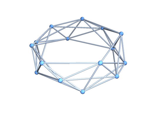
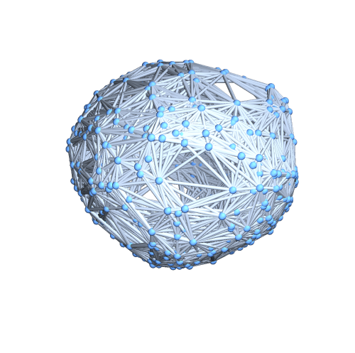
Figure 1. A non-standard model of a $d$-manifold is obtained by picking a large set $V$ of points and an $\delta>0$ which models machine precision and where $|V|$ is much larger than $1/\delta^{d}$. Define the graph $\Gamma=(V,E)$, where $(a,b)$ is in $E$ if $|b-a|<\delta$. The Whitney complex $G$ of this graph has a large dimension but a geometric realization is homotopic to $M$ and the Euler characteristic of $G$ is the same than the Euler characteristic of $M$. We see in this figure a model for a circle and for a sphere (where 500 random points were chosen and connected if Euclidean distance is less than $1/2$).

4. Remarks

4.1.

The following general remark from [29] is worth citing verbatim. It is remarkable as goes far beyond just modeling differential equations and somehow justifies an simple approach to the question of modeling ordinary differential equations using combinatorial models.

4.2.

Much of mathematics is intrinsically complex, and there is delight to be found in mastering complexity. But there can also be an extrinsic complexity arising from unnecessarily complicated ways of expressing intuitive mathematical ideas. Heretofore nonstandard analysis has been used primarily to simplify proofs of theorems. But it can also be used to simplify theories. There are several reasons for doing this. First and foremost is the aesthetic impulse, to create beauty. Second and very important is our obligation to the larger scientific community, to make our theories more accessible to those who need to use them.

4.3.

The motivations for the above set-up comes from various places: first of all from discrete Morse theory [5, 4, 3] which stresses the importance of using simplicial complexes for defining vector fields (but defines combinatorial vector fields quite differently), simplicial sets [33] (which also is a very different approach) as well as digital spaces [6, 9, 2] which provides valuable frame work. There is also motivation from the study of discrete approximations to chaotic maps [31, 35, 25], previous theorems of Poincaré-Hopf type [11, 14, 16, 18], as well as internal set theory [27, 32, 28]. We might comment on the later more elsewhere. Let us illustrate this with a tale of chaos theory. But not with a differential equation but with a map.

4.4.

The Ulam map $T(x)=4x(1-x)$ is a member in the logistic family on the interval $[0,1]$. It is topologically conjugated to the tent map and measure theoretically conjugated to the map $x\to 2x$ on the circle $\mathbb{T}^{1}$ and so Bernoulli, allowing to produce IID random variables. On any present computer implementation, the orbits of $T(x)=4x(1-x)$ and $S(x)=4x-4x^{2}$ disagree: $S^{60}(0.4)\neq T^{60}(0.4)$. Mathematica for example which computes with 17 digits machine precision,

${\rm T[x\_]:=4x(1-x);S[x\_]:=4x-4x^{2};\{NestList[T,0.4,60],NestList[S,0.4,60]\}}$

we compute $S^{60}(0.4)=0.715963$ and $T^{60}(0.4)=0.99515$. More dramatically, while $T^{4}(0.4)=S^{4}(0.4)$, the computer algebra system reports that $T^{5}(0.4)\neq S^{5}(0.4)$. Already computing the polynomial $T^{5}$ of degree $32$ produces different numbers because the integer coefficients of $T^{5}$ have more than 17 digits, while $T^{4}$ still has less than 17 digits so that the computer can still with it faithfully. With a Lyapunov exponent of $\log(2)$, the error of $T$ or $S$ gets doubled in each step so that $2^{60}\times\epsilon$ is larger than $10$ for the given machine precision $\epsilon=10^{-17}$ and because $4x-4x^{2}$ is only in the same $10^{-17}$ neighborhood of $4x(1-x)$, we get different numbers after 60 iterations. Floating point arithmetic does not honor the distributivity law.

4.5.

The simplicial complex $G$ in this case is any set of “machine numbers” in $[0,1]$ with the property that their mutual distance is smaller than $10^{-17}$. We have given the example of a map, but the same can happen for differential equations like the Lorenz system in $\mathbb{R}^{3}$, where techniques like finding horse shoes enable to prove that the system has invariant measures on the Lorenz attractor which the dynamics is a Bernoulli system. Also here, integrating the differential equation is better modeled microscopically as a map $F$ from a finite set $V$ to a simplicial complex $x\in G$ on $V$, rather then selecting a choice $F(x)\in V$. Yes, this defines a deterministic map on $V$ but it also defines a deterministic map on $G$, where the transition $x\to y$ is possible if $x$ and $y$ intersect. Choosing projections $G\to V$ by picking a point in the center is a good model what happens in a real computer.

4.6.

When investigating definitions of vector fields on graphs, we also aim for a Lie algebra structure. We have defined in [19] an algebraic notion of vector field $X$ as a rule $i_{X}:\Lambda^{p+1}\to\Lambda^{p}$ balancing the exterior derivative $d:\Lambda^{p}\to\Lambda^{p+1}$ on discrete forms producing a Lie derivative $L_{X}=i_{X}d+di_{X}=D_{X}^{2}$ for which the wave equation $u_{tt}=L_{X}u$ is solved by a d’Alembert type Schrödinger solution $e^{iD_{X}t}$ which classically is a Taylor theorem for transport. The point of the magic formula of Cartan is that it produces a transport flow on $p$ forms. If $i_{X}$ is replaced by $d^{*}$ we get the wave equation on $p$-forms. In spirit this is is similar as the flow of $L_{X}$ produces a dynamics using neighboring spaces of simplicial complexes. This is also the case for the Laplacian $L=d^{*}d+dd^{*}$, where now the deterministic $i_{X}$ is replaced by a diffusion process defined by $d^{*}$. So, also in this model, there is a deterministic flow version $L_{X}$ which classically is given by a vector field $X$ or a diffusive flow version $L$, in which case in some sense, we average over all possible vector fields. The dynamics approach via discrete Lie derivatives is different from the combinatorial one considered here and there is no Poincaré-Hopf theorem yet in the Lie derivative case.

4.7.

Poincaré-Hopf was generalized [23] to a function identity

$$f_{G}(t)=1+t\sum_{x\in V}f_{S_{g}(x)}(t)$$

for the generating function $f_{G}(t)=1+f_{0}t+\dots+f_{d}t^{d+1}$ encoding the $f$-vector of $G$, where $f_{k}$ is the number of $k$ dimensional sets in $G$. Averaging the index over some probability space of functions gives then curvature $K(x)$ satisfying Gauss-Bonnet $\chi(G)=\sum_{x}K(x)$. [13, 12, 15]. In the case of a uniform measure, the Gauss-Bonnet formula generalizes to the functional formula $f_{G}(t)=1+\sum_{x}F_{S(x)}(t)$, where $F_{G}(t)$ is the anti-derivative of $f_{G}$ [10, 20].

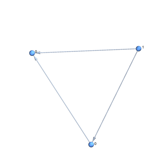
Figure 2. A cyclic triangle has zero integer Poincaré-Hopf index at every vertex as it has to add up to $1$ and symmetry requires the index to be the same on each vertex. If the vector field is acyclic, it comes from a gradient field, then an index function exists. It is $1$ at the minimum and $0$ else.

5. Irrotational digraphs

5.1.

This note started with the quest to generalize Poincaré-Hopf theorem [30, 7, 34] from gradient fields to more general vector fields. This problem has already been posed in [11] and it was pointed out that using a digraph alone can not work because a circular triangle produces an index inside. It turns out that the existence of such triangles is the only obstacle. We call digraphs without circular triangles irrotational. Such graphs still can have circular loops. We just don’t want to have them microscopically to happen on triangles.

5.2.

Let $\Gamma=(V,E)$ be a finite simple graph and $G$ the Whitney complex consisting of all finite simple subgraphs. If the edges of $\Gamma$ are oriented, we have a directed graph which is also called a digraph. Let $F$ be a $1$-form, a function from edges to $\mathbb{R}$ and the curl $dF=0$ is zero on all triangles, we can define

$$i_{F}(x)=1-\chi(S_{F}(x))\;,$$

where $S_{F}(x)=\{y\in S(x)$, for which $F$ points from $x$ to $y\}$. As we only need the direction of $F$ and not the magnitudeof the field, all what matters is a digraph structure on $G$.

5.3.

Let us call a finite simple digraph irrotational if there are no closed loops of length $3$ in the digraph. This does not mean that the graph is acyclic. Indeed, any one-dimensional graph (a graph with no triangles) and especially the cyclic graphs $C_{n}$ with $n\geq 4$ are irrational because there are no triangles to begin with. For an irrational graph we can then define a positive function $F:E\to\mathbb{R}$ on the oriented edges of the graph such that the curl satisfies $dF=0$. This justifies the name irrotational for the directed graph.

5.4.

Even if $F$ has zero curl, the field $F$ does not necessarily come from a scalar field $g$, as the first cohomology group $H^{1}(G)$ is not assumed to be trivial. Indeed $H^{1}(F)$ is the quotient of the vector space $\{F\;dF=0\}$ divided by the vector space $\{F=dg\}$ of gradient fields. More generally, the maps $G\to H^{k}(G)$ are functors from finite simple graphs to finite dimensional vector spaces and $b_{k}(G)={\rm dim}(H^{k}(G))$ are the Betti numbers of $G$ which satisfy $\sum_{k}(-1)^{k}b_{k}=\chi(G)$. The Euler characteristic of a digraph is the Euler characteristic of the finite simple graph in which the direction structure on the edges is forgotten.

5.5.

But Poincaré-Hopf still works in the irrotational case. The Euler characteristic of when the digraph structure is discarded.

Proposition 1 (Poincaré-Hopf for irrotational digraph).

Let $G$ be a finite simple irrotational digraph, then the index $i(x)=1-\chi(S^{-}(x))$ satisfies $\sum_{x}i(x)=\chi(G)$.

Proof.

Let $v$ be a vertex in $G$. The unit ball $B(v)$ is contractible and so has trivial cohomology. Since the digraph structure is irrotational, we can place function values $F(e)$ on the oriented edges of $G$ such that the curl of $F$ is zero in every triangle of $B(v)$. The field $F$ is therefore a gradient field. Since $H^{1}(B(v))=0$, there is a function $g$ such that the gradient of $g$ is $dg=F$. Now, the index at $v$ is the same than the usual index of $g$. ∎

5.6.

Example: The cyclic digraph graph $G=(\{1,2,3,4\},\{(12),(23),(34),(41)\})$ has $i(x)=0$ for all $x$. In contrast, for a gradient field $F=dF$ we always had at least two critical points: the local minima has index $1$ while the local maxima has index $-1$. In general, there are vector fields on any $d$ dimensional flat torus which have no critical point at all.

5.7.

The example of a triangle which has Euler characteristic $1$ shows that one can not get a local integer-valued index function on the vertices $x$ alone if one insists the index function to be deterministic and depend only on the structure of $F$ of the unit ball of $x$.

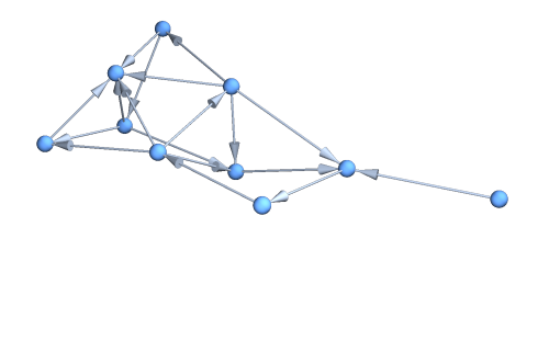
Figure 3. Example of acyclic graphs, digraphs in which no triangle is cyclic. As we can tune the values of a one form implementing the directions so that the curl is zero in each triangle, this 1-form is actually given locally by a gradient field defined by a potential function $g$. Not globally because of cohomology but the index is then the index of the locally injective function $g$.

5.8.

Example: Given a graph $G$ equipped with a direction field, we can look at the Barycentric refinement $G_{1}$ of $G$. The vertices are the simplices of $G$ and two are connected if one is contained in the other. If $e=a\to b$ is refined, we define a direction on $e_{1}:a\to b\to c$, keeping the flow there in the same direction. For any other new connection $x\to y$, keep flowing to the lower dimensional part. This vector field on $G_{1}$ has no cycles so that the above result holds for the Barycentric refined field.

Figure 4. The Barycentric refinement of the circular triangle splits each edge into two, leaves the direction there and connects the newly added simplex to all the vertices. This Barycentric refined field is always acyclic so that the above proposition applies.

Lemma 1.

The Barycentric refined field $F$ is acyclic.

Corollary 2.

The Poincaré-Hopf index function defined by a field $F$ adds up to the Euler characteristic.

Figure 5. A directed wheel graph and its Barycentric refinement. The later is irrotational so that we can assign Poincar e-Hopf indices to its vertices.

5.9.

Given a simplex $x=(x_{0},\cdots,x_{k})$ in a graph, a local Barycentric refinement at $x$ adds a new vertex $x$ and connects it to all points in $S(x)=S(x_{0})\cap\cdots\cap S(x_{k})$, where $S(x_{k})$ are the unit spheres of $S_{k}$ as well as all points $x_{k}$. We use it here for triangle refinements when $k=2$.

5.10.

There are two ways to think about the refinement. We can stay in the category of graphs but this changes the maximal dimension of the Whitney simplicial complex defined by $G$. If $x$ has dimension larger than $1$, We can also interpret it as a refinement of simplicial complexes and keep so the dimension the same. For example, if $G$ is a single triangle, then refining it we can within graph theory see the result as a 3-simplex with $f$-vector $(4,6,4,1)$. When getting rid of the original simplex, we have a complex with $3$ triangles and $6$ vertices and have an $f$-vector $(3,6,4)$. For $k=1$, the later version gives an edge refinement which when reversed is edge collapse. In general, we have:

Lemma 2.

Any local Barycentric refinement $G\to G_{1}(x)$ at a simplex $x$ preserves Euler characteristic.

Proof.

If $k$ is even, then the boundary sphere complex $S(x)$ has Euler characteristic $0$, the same number of even and odd dimensional simplices. When adding a new vertex, every odd simplex in $S(x)$ adds an even dimensional simplex in $G_{1}(x)$ and every even simplex in $S(x)$ adds an odd dimensional simplex in $G_{1}(x)$. We also add a $(k+1)$-dimensional simplex $(x,x_{0},...,x_{k})$ and a zero dimensional one which cancel. If $k$ is odd, then the boundary sphere complex $S(x)$ has Euler characteristic $2$, There are 2 more even dimensional simplices than odd dimensional ones. This means we add $2$ more odd dimensional simplices to $G_{1}(x)$ than odd dimensional ones. But we also add an even dimensional $(k+1)$ simplex $(x,x_{0},\cdots,x_{k})$ and vertex $x$. In total, we again do not change the balance of even and odd dimensional simplices, what the Euler characteristic is. ∎

5.11.

Given a graph $G$ and a field $F$, we make a local Barycentric refinement to every cyclic triangle $x$ in $G$ and make every arrow from the new vertex $x$ go away from $x$. Now, all triangles are acyclic and we can use the proposition to get an index. The index function is $1$ on triangles which are cyclic and $0$ else. The index of a vertex $v\in V$ is defined as

$$i_{F}(v)=1-\chi(S^{-}_{1}(v))$$

where $S_{1}^{-}(v)=\{w\in S_{1}(x)\;F$ points from $v$ to $w\}$ and $S_{1}(v)$ is the unit sphere in the Barycentric refined case.

5.12.

An other possibility to break a cyclic triangle is to make an edge refinement at one of the edges. Similarly as the triangle refinement, also this refinements depend in general on the order in which the refinements are done.

6. Averaging fields

6.1.

When averaging the Poincaré-Hopf indices over a probability space of locally injective functions $g$, we got curvature. The curvature depends on the probability measure. Having choice in averaging produces flexibility which allows to implement natural curvatures for convex polyhedra. Instead of averaging over all possible functions $g$, we could also average over all possible base maps $F:G\to V$. If for every simplex $x\in G$, and every $v\in x$ the probability that $F(x)=v$ is independent of $v$, then we get a curvature.

6.2.

The old story can can be understood as starting with an energy $\omega(x)=(-1)^{{\rm dim}(x)}$ on the simplices of the graph, for which $\sum_{x}\omega(x)=\chi(G)$ is the definition of Euler characteristic. The energy $\omega(x)$ is the Poincaré-Hopf index of the dimension function ${\rm dim}$ on the vertex set of the Barycentric refinement of $G$. The Poincaré-Hopf index $i_{G}(x)$ of the original graph with respect to some function $g$ is then obtained by moving every energy from a simplex $x$ to the vertex in $x$, where $g$ is maximal. One gets the curvature of $G$ by distributing the energy $\omega(x)$ equally to every vertex of $x$.

6.3.

If the field $F$ is irrational, then it is a gradient field in every simplex. There is therefore an ordering of the simplices. The process of distributing the value $\omega(x)$ of a simplex to the largest vertex in that ordering produces the index.

6.4.

Here is a remark. Let $\Omega$ be the probability space of all fields $F$ which are irrotational. Put the uniform measure on it and call $E[\cdot]$ the expectation. Denote by

$$K(x)=1+\sum_{k=0}(-1)^{k}f_{k}(S(x))/(k+1)$$

the Levitt curvature on the vertices of the graph, where $f_{k}(A)$ counts the number of $k$-dimensional simplices of $A$ and $S(x)$ is the unit sphere.

Lemma 3.

${\rm E}[i_{g}]=K$.

Proof.

We only have to show that for every simplex $x$, and every two vertices $v,w$ in $x$ the probability that $v$ is the largest element in $F$ is the same than that $w$ is the largest element. ∎

7. The hyperbolic case

7.1.

The discussion about Non-standard analysis should already indicate why every result which holds in the continuum also has an analogue in the discrete. Discrete Morse theory and especially [3] illustrates this. This is no surprise as a geometric realization of a discrete simplicial complex is a continuum space with the same features. Still, one has to look at the discrete case independent of the continuum and investigate how results from the continuum can be obtained without geometric realization.

7.2.

Let us start with a special Morse case which been mentioned a couple of times: if $G$ is a simplicial complex, we can define a graph $\Gamma=(V,E)$ where $V$ are the set of vertices in $G$ and $E$ the set of pairs $(x,y)$ with either $x\subset y$ or $y\subset x$. The Whitney complex $G_{1}$ of $\Gamma$ is called the Barycentric refinement of $G$. There is a natural choice for every simplex $x$ in $G_{1}$. It is the maximal simplex $v$ in $x$. In that case, $i_{F}(x)=(-1)^{{\rm dim}}(x)$ and every vertex is a critical point. The Poincaré-Hopf theorem then just tells that the Euler characteristic of the Barycentric refinement $G_{1}$ is the same than the Euler characteristic of $G$.

7.3.

The notion of discrete manifolds can be formulated elegantly in an inductive way. A $d$-graph is a finite simple graph for which all unit spheres $S(x)$ are $(d-1)$-spheres. A $d$-sphere $G$ is a $d$-graph such that $G-x$ is contractible for some $x\in G$. A graph is contractible if there exists $x$ such that $S(x)$ and $G-x$ are both contractible. The inductive definitions are primed by the assumption that the empty graph $0$ is the $(-1)$-sphere and $1=K_{1}$ is contractible. In this case, we have defined a function $g:V\to\mathbb{R}$ to be Morse, if the central manifolds $B_{g}(x)$ at every point are either empty, a sphere or a product of two spheres. In that case the symmetric index $j(x)=[i_{g}(x)+i_{-g}(x)]/2$ is given in terms of the central manifold [12].

7.4.

For a Morse function $g$, the gradient flow $x^{\prime}=\nabla g(x)$ is a hyperbolic system. The generalization in the continuum to $d$-dimensional smooth manifold is given by the Sternberg-Grobman-Hartman linearization theorem assures that new a hyperbolic equilibrium point $x$ of a differential equation $x^{\prime}=F(x)$, the stable and unstable manifolds $W^{\pm}(x)$ intersect a small sphere $S_{r}(x)$ in $m-1$ and $(d-m-1)$-dimensional spheres. The Poincaré-Hopf index $i_{F}(x)$ is $(-1)^{m}$, where $m=m(x)$ is the Morse index, the dimension of the stable manifold at $x$. Poincaré-Hopf is then usually formulated as $\chi(M)=\sum_{k}(-1)^{k}c_{k}$, where $c_{k}$ is the number of equilibria with Morse index $k$. By using the dynamics to build a cell complex, one has also a bound on the Betti numbers $b_{m}\leq c_{m}$.

7.5.

In discrete set-up, we have to assume a bi-directed complex which comes from a $d$-graph. For every $v\in V$ we have subsets $F^{\pm}(v)\subset G$. A vector field is then called hyperbolic if for every $v$ for which $F^{\pm}(v)$ is not contractible, the sets $F^{-}(v)$ is homotopic to a $(m-1)$-sphere and $F^{+}(v)$ to a $d-m-1$ sphere and that the join of these two spheres is homotopic to a $(d-1)$-sphere, the unit sphere in $M$. For example, in the case $d=2$, we have either sinks with $m=2$, sources with $d=0$ or hyperbolic saddle points with $m=1$. In the later case, the sets $F^{\pm}(x)$ are homotopic to the zero sphere and the join of these two zero spheres is a 1-sphere. Note however, that the Betti inequalities $b_{m}\leq c_{m}$ are no more true in general (this is the same as in the continuum). For a circle for example, there are vector fields without any critical points. The Betti of the circle are however $b_{0}=1,b_{1}=1$. It is only in the case of gradient fields that we always have a critical point of index $m=0$ (a minimum) and a critical point with index $m=1$ (a maximum). The Reeb sphere theorem (see [24] for a discussion in the discrete) assures that spheres are characterized by the existence of Morse functions with exactly two critical points.

References

- [1] P. Dlotko and H. Wagner. Simplification of complexes of persistent homology computations. Homology, Homotopy and Applications, 16:49–63, 2014.
- [2] A.V. Evako. The Jordan-Brouwer theorem for the digital normal n-space space . http://arxiv.org/abs/1302.5342, 2013.
- [3] R. Forman. Combinatorial vector fields and dynamical systems. Math. Z., 228(4):629–681, 1998.
- [4] R. Forman. Morse theory for cell complexes. Adv. Math., page 90, 1998.
- [5] R. Forman. Combinatorial differential topology and geometry. New Perspectives in Geometric Combinatorics, 38, 1999.
- [6] G.T. Herman. Geometry of digital spaces. Birkhäuser, Boston, Basel, Berlin, 1998.
- [7] H. Hopf. Vektorfelder in -dimensionalen Mannigfaltigkeiten. Math. Ann., 96(1):225–249, 1927.
- [8] O.E. Lanford III. An introduction to computers and numerical analysis. In Phénomènes critiques, systèmes aléatoires, thóries de jauge, Part I, II, Les Houches, 1984, pages 1–86. North-Holland, Amsterdam, 1986.
- [9] A.V. Ivashchenko. Graphs of spheres and tori. Discrete Math., 128(1-3):247–255, 1994.
-
[10]
O. Knill.
A graph theoretical Gauss-Bonnet-Chern theorem.
http://arxiv.org/abs/1111.5395, 2011. -
[11]
O. Knill.
A graph theoretical Poincaré-Hopf theorem.
http://arxiv.org/abs/1201.1162, 2012. -
[12]
O. Knill.
An index formula for simple graphs .
http://arxiv.org/abs/1205.0306, 2012. -
[13]
O. Knill.
On index expectation and curvature for networks.
http://arxiv.org/abs/1202.4514, 2012. -
[14]
O. Knill.
The theorems of Green-Stokes,Gauss-Bonnet and Poincare-Hopf in Graph
Theory.
http://arxiv.org/abs/1201.6049, 2012. -
[15]
O. Knill.
The Euler characteristic of an even-dimensional graph.
http://arxiv.org/abs/1307.3809, 2013. -
[16]
O. Knill.
Classical mathematical structures within topological graph theory.
http://arxiv.org/abs/1402.2029, 2014. -
[17]
O. Knill.
On Fredholm determinants in topology.
https://arxiv.org/abs/1612.08229, 2016. -
[18]
O. Knill.
The amazing world of simplicial complexes.
https://arxiv.org/abs/1804.08211, 2018. -
[19]
O. Knill.
Cartan’s magic formula for simplicial complexes.
https://arxiv.org/abs/1811.10125, 2018. -
[20]
O. Knill.
Dehn-Sommerville from Gauss-Bonnet.
https://arxiv.org/abs/1905.04831, 2019. -
[21]
O. Knill.
Energized simplicial complexes.
https://arxiv.org/abs/1908.06563, 2019. -
[22]
O. Knill.
The energy of a simplicial complex.
https://arxiv.org/abs/1907.03369, 2019. -
[23]
O. Knill.
A parametrized Poincare-Hopf theorem and clique cardinalities of
graphs.
https://arxiv.org/abs/1906.06611, 2019. -
[24]
O. Knill.
A Reeb sphere theorem in graph theory.
https://arxiv.org/abs/1903.10105, 2019. - [25] Oscar E. Lanford, III. Informal remarks on the orbit structure of discrete approximations to chaotic maps. Experiment. Math., 7(4):317–324, 1998.
- [26] G. F. Lawler. Comments on edward nelson’s internal set theory: a new approach to nonstandard analysis. Bulletin (New Series) of the AMS, 4:503–506, 2011.
- [27] E. Nelson. Internal set theory: A new approach to nonstandard analysis. Bull. Amer. Math. Soc, 83:1165–1198, 1977.
- [28] E. Nelson. Radically elementary probability theory. Princeton university text, 1987.
- [29] E. Nelson. The virtue of simplicity. In The Strength of Nonstandard Analysis, pages 27–32. Springer, 2007.
- [30] H. Poincaré. Sur les courbes définies par les équations differentielles. Journ. de Math, 4, 1885.
- [31] F. Rannou. Numerical study of discrete area-preserving mappings. Acta Arithm, 31:289–301, 1974.
- [32] A. Robert. Analyse non standard. Presses polytechniques romandes, 1985.
- [33] A. Romero and F. Sergeraert. Discrete vector fields and fundamental algebraic topology. Version 6.2. University of Grenoble, 2012.
- [34] M. Spivak. A comprehensive Introduction to Differential Geometry I-V. Publish or Perish, Inc, Berkeley, third edition, 1999.
- [35] X-S. Zhang and F. Vivaldi. Small perturbations of a discrete twist map. Ann. Inst. H. Poincaré Phys. Théor., 68:507–523, 1998.