Compositional Hierarchical Tensor Factorization:
Representing Hierarchical Intrinsic and Extrinsic Causal Factors

Abstract.

Visual objects are composed of a recursive hierarchy of perceptual wholes and parts, whose properties, such as shape, reflectance, and color, constitute a hierarchy of intrinsic causal factors of object appearance. However, object appearance is the compositional consequence of both an object’s intrinsic and extrinsic causal factors, where the extrinsic causal factors are related to illumination, and imaging conditions.Therefore, this paper proposes a unified tensor model of wholes and parts, and introduces a compositional hierarchical tensor factorization that disentangles the hierarchical causal structure of object image formation, and subsumes multilinear block tensor decomposition as a special case. The resulting object representation is an interpretable combinatorial choice of wholes’ and parts’ representations that renders object recognition robust to occlusion and reduces training data requirements. We demonstrate our approach in the context of face recognition by training on an extremely reduced dataset of synthetic images, and report encouraging face verification results on two datasets – the Freiburg dataset, and the Labeled Face in the Wild (LFW) dataset consisting of real-world images, thus, substantiating the suitability of our approach for data starved domains.

1. Introduction

Statistical data analysis that disentangles the causal factors of data formation and computes a representation that facilitates the analysis, visualization, compression, approximation, and/or interpretation of the data is challenging and of paramount importance.

“Natural images are the composite consequence of multiple constituent factors related to scene structure, illumination conditions, and imaging conditions. Multilinear algebra, the algebra of higher-order tensors, offers a potent mathematical framework for analyzing the multifactor structure of image ensembles and for addressing the difficult problem of disentangling the constituent factors or modes.” (Vasilescu and Terzopoulos, $2002$ (vasilescu02, ))

Scene structure is composed from a set of objects that appear to be formed from a recursive hierarchy of perceptual wholes and parts whose properties, such as shape, reflectance, and color, constitute a hierarchy of intrinsic causal factors of object appearance. Object appearance is the compositional consequence of both an object’s intrinsic causal factors, and extrinsic causal factors with the latter related to illumination (i.e. the location and types of light sources), imaging (i.e. viewpoint, viewing direction, lens type and other camera characteristics). Intrinsic and extrinsic causal factors confound each other’s contributions hindering recognition.

“Intrinsic properties are by virtue of the thing itself and nothing else” (David Lewis, 1983 (Lewis1983a, )); whereas an extrinsic properties are not entirely about that thing, but as result of the way the thing interacts with the world. Unlike global intrinsic properties, local intrinsic properties are intrinsic to a part of the thing, and it may be said that a local intrinsic property is in an “intrinsic fashion”, or “intrinsically” about the thing, rather than “is intrinsic” to the thing (Humberstone1996, ; Figdor2008, ). David Lewis (Lewis1983a, ) provides a formal discussion of intrinsic and extrinsic concepts of causality and addresses a few related distinctions that an intuitive definition conflates, such as local versus global intrinsic properties, duplication preserving properties, and interior versus exterior properties. The meaning of intrinsic and extrinsic causation was extensively explored in philosophy, philosophy of mind, metaphysics and philosophy of physics (Hume1748, ; Lewis1973, ; Lewis1983a, ; Menzies1999, ; pearl00, ).

Our goal is to explicitly represent local and global intrinsic causal factors as statistically invariant representations to all other causal factors of data formation.

Historically, statistical object recognition paradigms can be categorized based on how object structure is represented and recognized, ie. based on the appearance of an object’s local features (Wong2012, ; Gao2010, ), or based on the overall global object appearance (Heisele2003, ; Shakhnarovich04, ; Bartlett02, ; Yang2001, ; Martinez2001, ; belhumeur1997, ; Turk91b, ). Both approaches have strengths and shortcomings. Global features are sensitive to occlusions, while local features are sensitive to local deformations and noise. A hybrid approach that employs both global object features, and local features mitigates the shortcoming of both approaches (Li2015, ; Murphy2006, ; xu08, ).

Deep learning methods, which have become a highly successful approach for object recognition, compute feature hierarchies composed of low-level and mid-level features either in a supervised (lecun98, ), unsupervised (hinton06, ; larochelle07, ; ranzato06, ) or semi-supervised manner (nair09, ). This has been achieved by composing modules of the same architectures, such as Restricted Boltzmann Machines (hinton06, ), autoencoders (larochelle07, ), or various forms of encoder-decoder networks (ranzato06, ; Cadieu09, ; Jarrett09, ).

Cohen et al.’s  (cohen16, ; cohen16b, ) theoretical results show that convolutional neural networks (CNNs) are theoretically equivalent in their representational power to hierarchical Tucker factorization  (hackbusch2009, ; Grasedyck2010, ; perros15, ; oseledets11, ), and shallow networks are equivalent to linear tensor factorizations, aka CANDECOMP/Parafac (CP) tensor factorization (Carroll70, ; Harshman70, ; Bro97, ). Vasilescu and Terzopoulos (Vasilescu01b, )(vasilescu02, )(Vasilescu03, )(Vasilescu05, )(Vasilescu2011, ) demonstrated that tensor algebra is a suitable, interpretable framework for mathematically representing and disentangling the causal structure of data formation in computer vision, computer graphics and machine learning  (Vasilescu05, ; Vasilescu09, ), Figure 1. Problem setup and implementation differences between CNNs and our tensor algebraic approach impact interpretability, data needs, memory/storage and computational complexity, often rendering CNN models difficult to deploy on mobile devices, or any devices with limited computational resources.

Inspired and inspirited by Cohen et al.’s (cohen16, ; cohen16b, ) theoretical results, and by the TensorFaces and Human Motion Signatures approach  (vasilescu02, ; Vasilescu03, ; Vasilescu01b, ; Vasilescu02b, ), we propose a unified tensor model of wholes and parts based on a reconceptualization of the data tensor as a hierarchical data tensor, a mathematical representation of a tree data-structure. Defining a hierarchical data tensor enables a single elegant mathematical model that can be optimized in a principled manner instead of employing a myriad of individual part-based engineering solutions that independently represent each part and attempt to compute all possible dimensionality reduction permutations. Our factorization optimizes simultaneously across all the wholes and parts of the hierarchy, learns a convolutional feature hierarchy of low-level, mid-level and high-level features, and computes an interpretable compositional object representation of parts and wholes. Our resulting object representation is a combinatorial choice of part representations, that renders object recognition robust to occlusion while bypassing large training data requirements.

Our compositional tensor factorization and learnt feature hierarchy is also applicable to CNNs. Since CNNs learn millions of parameters that may lead to redundancy and poor generalization, our factorization and dimensionality reduction approach may be employed to reparameterize and reduce a tensor of CNN parameters, potentially resulting in better generalization (Lebedev14, ; Novikov2015, ; Kim15, ; kossaifi17, ).

DeepFace, a CNN approach (Taigman2014, ; Huang2012, ; Sun2013, ; Chen2015, ; xiong2016, ), celebrated closing the gap on human-level performance for face verification by testing on the Labeled Faces in the Wild (LFW) database (Huang2007, ) of $13,233$ images from $5,749$ people in the news, and training on a large dataset of $4,400,000$ facial images from $4,030$ people, the same order of magnitude as the number of people in the test data set  (Parkhi15, ). This large training data resulted in an increase from $70\%$ verification rates to $97.35\%$.

The very resources that make deep learning a wildly successful approach today are also its shortcomings. In general, it is difficult and expensive to acquire large representative training data for object image analysis or recognition, and once acquired, there is a need for high performance computing, such as distributed GPU computing  (tensorflow2015-whitepaper, ; collobert2011torch7, ; Bastien-Theano-2012, ; bergstra+al:2010-scipy, ).

While we have not closed the gap on human performance, the expressive power of our representation and our verification results are promising. We demonstrate and validate our novel compositional tensor representation in the context of the face verification, albeit it is intended for any data verification or classification scenario. We trained on less than one percent ($1\%$) of the total images used by DeepFace. We trained on the images of only $100$ people and tested on the images of the $5,749$ people in the LFW database.

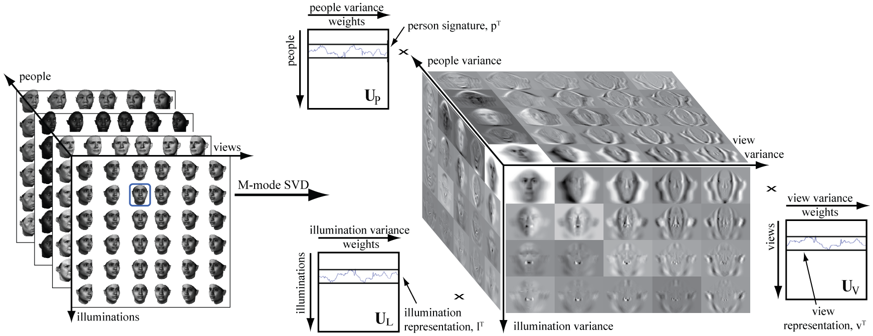
(a)                          No           No Cast Shadow         Original       Cast Shadow         No Shading                  (b)              (c)

Figure 1. (a) TensorFaces representation: This image illustrates a multilinear tensor factorization of a $4^{th}$-order training data tensor, ${\mathbf{\mathcal{D}}}\in\mathbb{R}^{I_{\mbox{\tiny{x}}}\times I_{\mbox{\tiny{L}}}\times I_{\mbox{\tiny{V}}}\times I_{\mbox{\tiny{P}}}}$ where $I_{\mbox{\tiny{x}}},I_{\mbox{\tiny{L}}},I_{\mbox{\tiny{V}}},I_{\mbox{\tiny{P}}}$ are the number of pixels, illuminations, views and people, respectively. A vectorized image, ${\mathbf{d}}$, is represented by a set of coefficient vectors, one for the illumination, viewpoint, and person, and expressed mathematically as ${\mathbf{d}}={\mathbf{\mathcal{T}}}\times_{\mbox{\tiny{L}}}{\mathbf{l}}^{\mathrm{T}}\times_{\mbox{\tiny{V}}}{\mathbf{v}}^{\mathrm{T}}\times_{\mbox{\tiny{P}}}{\mathbf{p}}^{\mathrm{T}}$, where the TensorFaces basis, ${\mathbf{\mathcal{T}}}$, governs the interaction between different causal factors of data formation. (Data should be centered, but for this display it was added back.) (b) These set of images demonstrate the models ability to disentangle the causal factors. Illumination effects, such as highlights, cast shadows and shading  (Vasilescu03, ) are predectively and progressively reduced. (c) Vlasic etal (Vlasic05, ) generate new images by performing multilinear expression re-targeting.

Contributions:

${\textbf{1}}.$ This paper (i) explicitly addresses the meaning of intrinsic versus extrinsic causality, and (ii) models cause-and-effect as multilinear tensor interaction between intrinsic and extrinsic hierarchical causal factors of data formation. The causal factor representations are interpretable, hierarchical, statistically invariant to all other causal factors and computed based on $2^{\hbox{\small nd}}$ order statistics, but may be extended to employ higher-order statistics, or kernel approaches.

${\textbf{2}}.$ In analogy to autoencoders which are inefficient and approximate neural network implementations of principal component analysis, a pattern analysis method based in linear algebra, CNNs are neural network implementations of tensor factorizations.

This paper contributes to the tensor algebraic paradigm: (i) we express our data tensor in terms of a unified tensor model of wholes and parts by defining a hierarchical data tensor; (ii) we introduce a compositional hierarchical tensor factorization that subsumes block-tensor decomposition as a special case (DeLathauwer08, ; Delathauwer08c, ); (iii) we validate our approach by employing our new compositional hierarchical tensor factorization in the context of face recognition, but it may be applied to any type of data.This approach is data agnostic.

2. Relevant Tensor Algebra

We will use standard textbook notation,denoting scalars by lower case italic letters $(\it{a,b,...})$, vectors by bold lower case letters $({\mathbf{a,b,...}})$, matrices by bold uppercase letters $({\textbf{A}},{\textbf{B}},...)$, and higher-order tensors by bold uppercase calligraphic letters $({\mathbf{\mathcal{A}}},{\mathbf{\mathcal{B}}},...)$. Index upper bounds are denoted by italic uppercase (i.e., $1\leq i\leq I$). The zero matrix is denoted by 0, and the identity matrix is denoted by I.

Briefly, a tensor, or $m$-way array, is a generalization of a vector (first-order tensor) and a matrix (second-order tensor). Tensors are multilinear mappings over a set of vector spaces. The order of tensor ${\mathbf{\mathcal{A}}}\in\mathbb{R}^{I_{1}\times I_{2}\times\dots\times I_{M}}$ is $M$. An element of ${\mathbf{\mathcal{A}}}$ is denoted as ${\mathbf{\mathcal{A}}}_{i_{1}\dots i_{m}\dots i_{M}}$ or $a_{i_{1}\dots i_{m}\dots i_{M}}$, where $1\leq i_{m}\leq I_{m}$. In tensor terminology, column vectors are referred to as mode-1 vectors and row vectors as mode-2 vectors. The mode-$m$ vectors of an $M^{\hbox{\small th}}$-order tensor ${\mathbf{\mathcal{A}}}\in\mathbb{R}^{I_{1}\times I_{2}\times\dots\times I_{M}}$ are the $I_{m}$-dimensional vectors obtained from ${\mathbf{\mathcal{A}}}$ by varying index $i_{m}$ while keeping the other indices fixed. The mode-$m$ vectors of a tensor are also known as fibers. The mode-$m$ vectors are the column vectors of matrix ${{\textbf{A}}}_{\mbox{\tiny{$[m]$}}}$ that results from matrixizing (a.k.a. flattening) the tensor ${\mathbf{\mathcal{A}}}$ (Fig. 2).

Definition 0 (Mode-$m$ Matrixizing).

The mode-$m$ matrixizing of tensor ${\mathbf{\mathcal{A}}}\in\mathbb{R}^{I_{1}\times I_{2}\times\dots I_{M}}$ is defined as the matrix ${{\textbf{A}}}_{\mbox{\tiny{$[m]$}}}\in\mathbb{R}^{I_{m}\times(I_{1}\dots I_{m-1}I_{m+1}\dots I_{M})}$. As the parenthetical ordering indicates, the mode-$m$ column vectors are arranged by sweeping all the other mode indices through their ranges, with smaller mode indexes varying more rapidly than larger ones; thus,

$$\hskip-28.90755pt\left[{{\textbf{A}}}_{\mbox{\tiny{$[m]$}}}\right]_{jk} \hskip-7.22743pt=a_{i_{1}\dots i_{m}\dots i_{M}},\quad\mbox{where}$$

$$\hskip-14.45377pt\quad j=i_{m}\quad\mbox{and}\quad k=1+\sum_{n=1\atop n\neq m}^{M}(i_{n}-1)\prod_{l=1\atop l\neq m}^{n-1}I_{l}.\vspace{-.2in}$$

A generalization of the product of two matrices is the product of a tensor and a matrix (Delathauwer00a, ).

Definition 0 (Mode-$m$ Product, $\times_{\mbox{\tiny{m}}}$).

The mode-$m$ product of a tensor ${\mathbf{\mathcal{A}}}\in\mathbb{R}^{I_{1}\times I_{2}\times\dots\times I_{m}\times\dots\times I_{M}}$ and a matrix ${\textbf{B}}\in\mathbb{R}^{J_{m}\times I_{m}}$, denoted by ${\mathbf{\mathcal{A}}}\times_{m}{\textbf{B}}$, is a tensor of dimensionality
$\mathbb{R}^{I_{1}\times\dots\times I_{m-1}\times J_{m}\times I_{m+1}\times\dots\times I_{M}}$ whose entries are

$$[{\mathbf{\mathcal{A}}}\times_{m}{\textbf{B}}]_{i_{1}\dots i_{m-1}j_{m}i_{m+1}\dots i_{M}}=\sum_{i_{m}}a_{i_{1}\dots i_{m-1}i_{m}i_{m+1}\dots i_{M}}b_{j_{m}i_{m}}.\vspace{-.05in}$$

The mode-$m$ product can be expressed in tensor notation, as ${\mathbf{\mathcal{C}}}={\mathbf{\mathcal{A}}}\times_{m}{\textbf{B}},$ or in terms of matrixized tensors, as ${{\textbf{C}}}_{\mbox{\tiny{$[m]$}}}={\textbf{B}}{{\textbf{A}}}_{\mbox{\tiny{$[m]$}}}.$ The $M$-mode SVD (aka. the Tucker decomposition) is a “generalization” of the conventional matrix (i.e., 2-mode) SVD which may be written in tensor notation as

(2) D $$\hskip-7.22743pt={\textbf{U}}_{1}{\textbf{S}}{\textbf{U}}_{2}^{\mathrm{T}}\hskip 16.26118pt\Leftrightarrow\hskip 14.45377pt{\textbf{D}}={\textbf{S}}\times_{1}{\textbf{U}}_{1}\times_{2}{\textbf{U}}_{2}.$$

The $M$-mode SVD orthogonalizes the $M$ spaces and decomposes the tensor as the mode-m product, denoted $\times_{m}$ , of $M$-orthonormal spaces, as follows:

(3) $$\hskip-21.68121pt{\mathbf{\mathcal{D}}} \hskip-7.22743pt={{\mathbf{\mathcal{Z}}}}\times_{1}{{\textbf{U}}}_{1}\times_{2}{{\textbf{U}}}_{2}\dots\times_{m}{{\textbf{U}}}_{m}\dots\times_{M}{{\textbf{U}}}_{M}.$$

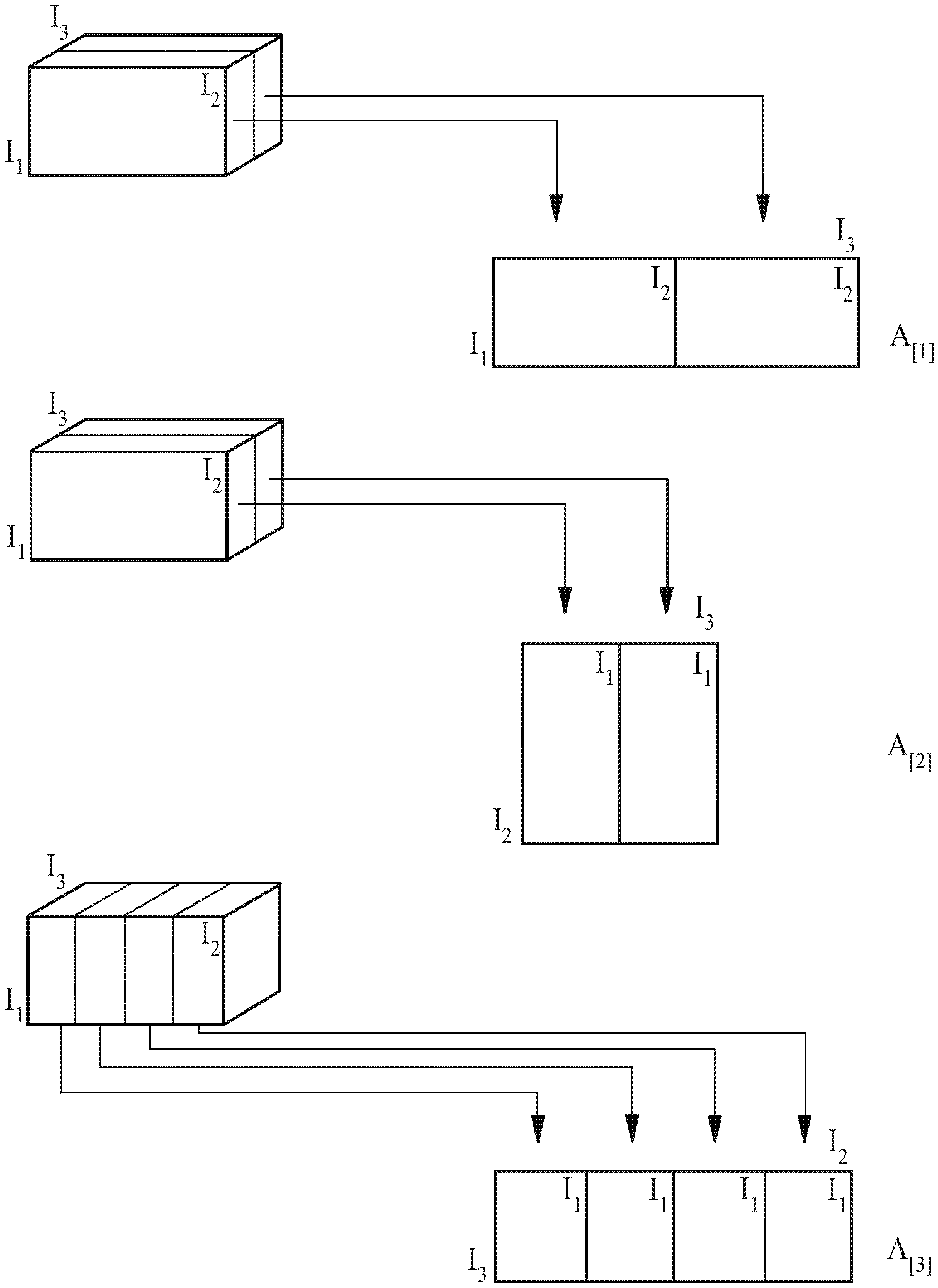
Figure 2. Matrixizing a (3rd-order) tensor. The tensor can be matrixized in 3 ways to obtain matrices comprising its 1-mode, 2-mode, and 3-mode vectors. Note that this matrixizing is not cyclical, unlike the one defined in  (Delathauwer00a, ).

Input the data tensor ${\mathbf{\mathcal{D}}}\in\mathbb{R}^{I_{1}\times\dots\times I_{M}}$.

1. For $m\mathrel{\mathop{:}}=1,\dots,M$,
   Let ${\textbf{U}}_{m}$ be the left orthonormal matrix of the SVD of ${{\textbf{D}}}_{\mbox{\tiny{$[m]$}}}$, the mode-$m$ matrixized ${\mathbf{\mathcal{D}}}$.

2. Set ${\mathbf{\mathcal{Z}}}\mathrel{\mathop{:}}={\mathbf{\mathcal{D}}}\times_{1}{\textbf{U}}_{1}^{\mathrm{T}}\times_{2}{\textbf{U}}_{2}^{\mathrm{T}}\dots\times_{m}{\textbf{U}}_{m}^{\mathrm{T}}\dots\times_{M}{\textbf{U}}_{M}^{\mathrm{T}}$.

Output mode matrices ${\textbf{U}}_{1},\dots,{\textbf{U}}_{M}$ and the core tensor ${\mathbf{\mathcal{Z}}}$.

Algorithm 1 $M$-mode SVD algorithm.

3. Global Tensor Factorization

There are two classes of data tensor modeling techniques (Kolda09, ; Sidiropoulo2017, ) that stem from: the rank-$K$ decomposition (CANDECOMP/Parafac decomposition) (Carroll70, ; Harshman70, ; Bro97, ) and the multilinear rank-($R_{\mbox{\tiny{1}}},R_{\mbox{\tiny{2}}},\dots,R_{\mbox{\tiny{M}}})$, such as Tucker decomposition (Tucker66, )(Delathauwer00a, )(desilva08, ), such as Multilinear-PCA, multilinear (tensor) ICA, plus various kernel variations that are doubly nonlinear (Vasilescu09, ).

3.1. Representation: Multilinear Tensor Factorization

Within the tensor mathematical framework, an ensemble of observations is organized in a higher order data tensor, ${\mathbf{\mathcal{D}}}$. Given a data tensor ${\mathbf{\mathcal{D}}}$ of labeled, vectorized training facial images ${\mathbf{d}}_{pvle}$, where the subscripts denote the causal factors of facial image formation, the person $p$, view $v$, illumination $l$, and expression $e$ labels, the $M$-mode SVD (Vasilescu03, )(Vasilescu02a, )(Delathauwer00a, )(DeLathauwer00b, ) or its kernel variant (Vasilescu09, ) may be employed to multilinearly decompose the data tensor,

(4) $${\mathbf{\mathcal{D}}}={\mathbf{\mathcal{T}}}\times_{\mbox{\tiny{P}}}{\textbf{U}}_{\mbox{\tiny{P}}}\times_{\mbox{\tiny{V}}}{\textbf{U}}_{\mbox{\tiny{V}}}\times_{\mbox{\tiny{L}}}{\textbf{U}}_{\mbox{\tiny{L}}}\times_{\mbox{\tiny{E}}}{\textbf{U}}_{\mbox{\tiny{E}}},$$

and compute the mode matrices ${\textbf{U}}_{\mbox{\tiny{P}}}$, ${\textbf{U}}_{\mbox{\tiny{V}}}$, ${\textbf{U}}_{\mbox{\tiny{L}}}$, and ${\textbf{U}}_{\mbox{\tiny{E}}}$ that span the causal factor representation. The extended core computed by, ${\mathbf{\mathcal{T}}}={\mathbf{\mathcal{D}}}\times_{\mbox{\tiny{P}}}{\textbf{U}}_{\mbox{\tiny{P}}}^{\mathrm{T}}\times_{\mbox{\tiny{V}}}{\textbf{U}}_{\mbox{\tiny{V}}}^{\mathrm{T}}\times_{\mbox{\tiny{L}}}{\textbf{U}}_{\mbox{\tiny{L}}}^{\mathrm{T}}\times_{\mbox{\tiny{E}}}{\textbf{U}}_{\mbox{\tiny{E}}}^{\mathrm{T}},$ governs the interaction between the causal factors (Figure 1). This approach makes the assumption that the representations for a causal factor are well modeled by a Gaussian distribution. An image ${\mathbf{d}}_{pvle}$ is represented by a person, view, illumination and expression coefficient vectors as,

(5) $${\mathbf{d}}_{pvle}={\mathbf{\mathcal{T}}}\times_{\mbox{\tiny{P}}}{\mathbf{p}}_{p}^{\mathrm{T}}\times_{\mbox{\tiny{V}}}{\mathbf{v}}_{v}^{\mathrm{T}}\times_{\mbox{\tiny{L}}}{\mathbf{l}}_{l}^{\mathrm{T}}\times_{\mbox{\tiny{E}}}{\mathbf{e}}_{e}^{\mathrm{T}}.$$

An important advantage of employing vectorized observations in a multilinear tensor framework is that all images of a person, regardless of viewpoint, illumination and expression are mapped to the same person coefficient vector, thereby achieving zero intra-class scatter. Thus, multilinear analysis creates well separated people classes by maximizing the ratio of inter-class scatter to intra-class scatter. Alternatively, one can employ the Multilinear (Tensor) Independent Component Analysis (MICA) algorithm  (Vasilescu05, ), $M$-mode ICA (as opposed to the tensorized computation of the conventional, linear ICA(Delathauwer97, )), which takes advantage of higher-order statistics (Common94, ) to compute the mode matrices that span the causal factor representation, and the MICA basis tensor that governs their interaction.

3.2. Recognition: Mutilinear Projection

While TensorFaces (MPCA) (vasilescu02, ; Vasilescu03, ) is a handy moniker for an approach that learns from an image ensemble the interaction and representation of various causal factors that determine observed data, with Multilinear (Tensor) ICA (Vasilescu05, ) as a more sophisticated approach, none of the interaction models prescribe a solution for how one might determine the causal factors of a single unlabeled test image that is not part of the training set. Multilinear projection (Vasilescu2011, ; Vasilescu07a, ) simultaneously projects one or more unlabeled test images that are not part of the training data set into multiple constituent causal factor spaces associated with data formation, in order to infer the mode labels:

(6) $$\vspace{-.25in}{{\mathbf{\mathcal{R}}}}={\mathbf{\mathcal{T}}}^{+\lower 2.0pt\hbox{\hskip-2.0pt\hbox{\tiny${}_{\mbox{\tiny{x}}}$}}}\times^{\hskip-1.0pt\hbox{\tiny{}T}}_{\mbox{\tiny{x}}}{{\mathbf{d}}}_{\mbox{\tiny{new}}}\approx{{\mathbf{r}}}_{\mbox{\tiny{P}}}\circ{{\mathbf{r}}}_{\mbox{\tiny{V}}}\circ{{\mathbf{r}}}_{\mbox{\tiny{L}}}\circ{\bf r}_{\mbox{\tiny{E}}}.\vspace{.275in}$$

The multilinear projection of a facial image computes the illumination, view and person representation by decomposing the expected rank-$1$ structure of the confounded response tensor ${{\mathbf{\mathcal{R}}}}$, and taking advantage of the unit vector constraints associated with ${{\mathbf{r}}}_{\mbox{\tiny{L}}}$, ${{\mathbf{r}}}_{\mbox{\tiny{V}}}$, ${{\mathbf{r}}}_{\mbox{\tiny{E}}}$, and ${{\mathbf{r}}}_{\mbox{\tiny{P}}}$. via the CP-decomposition, i.e., the rank-$1$ tensor decomposition.

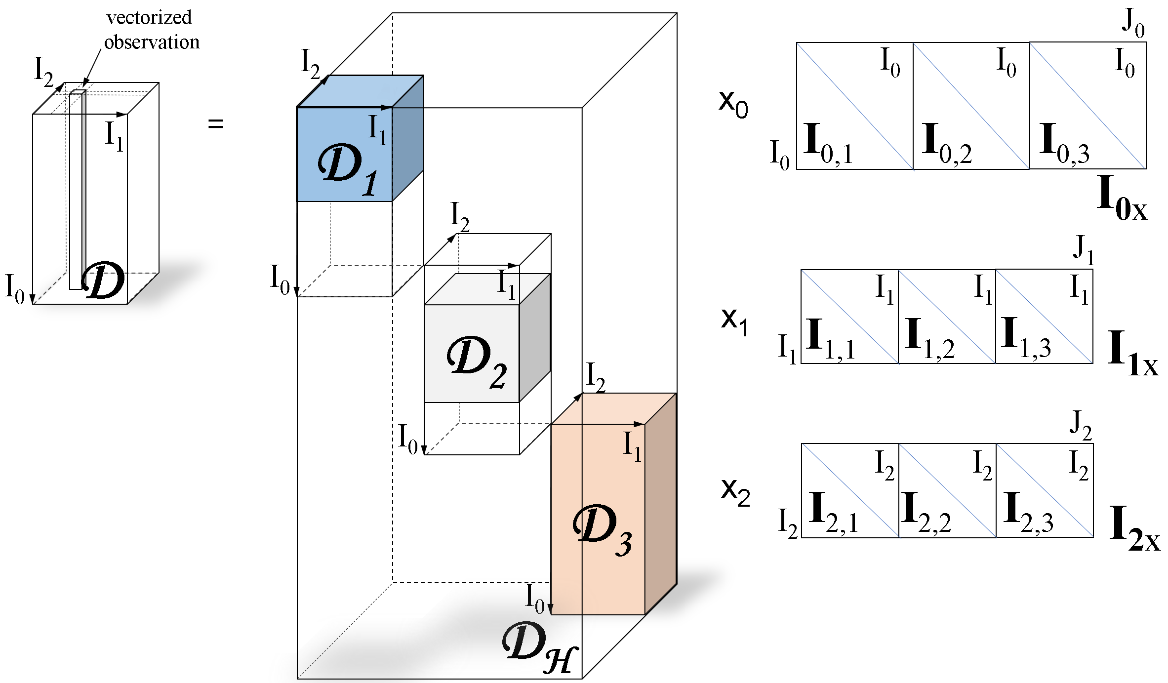
                                            (a) (b)

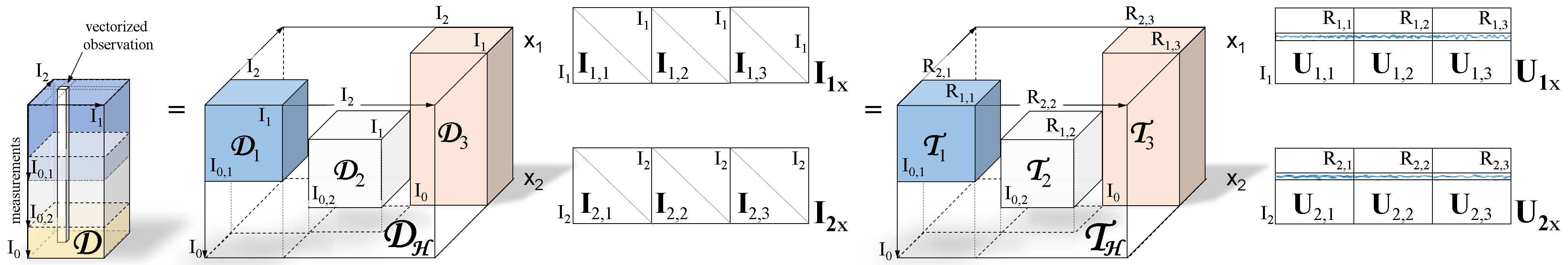
                                            (c1) (c2)

     

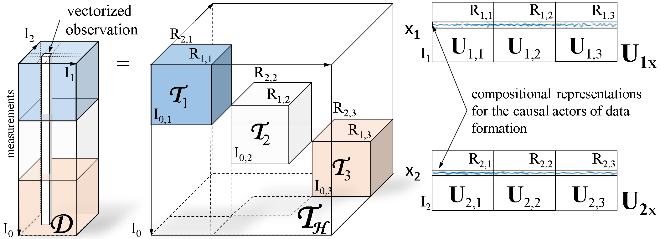
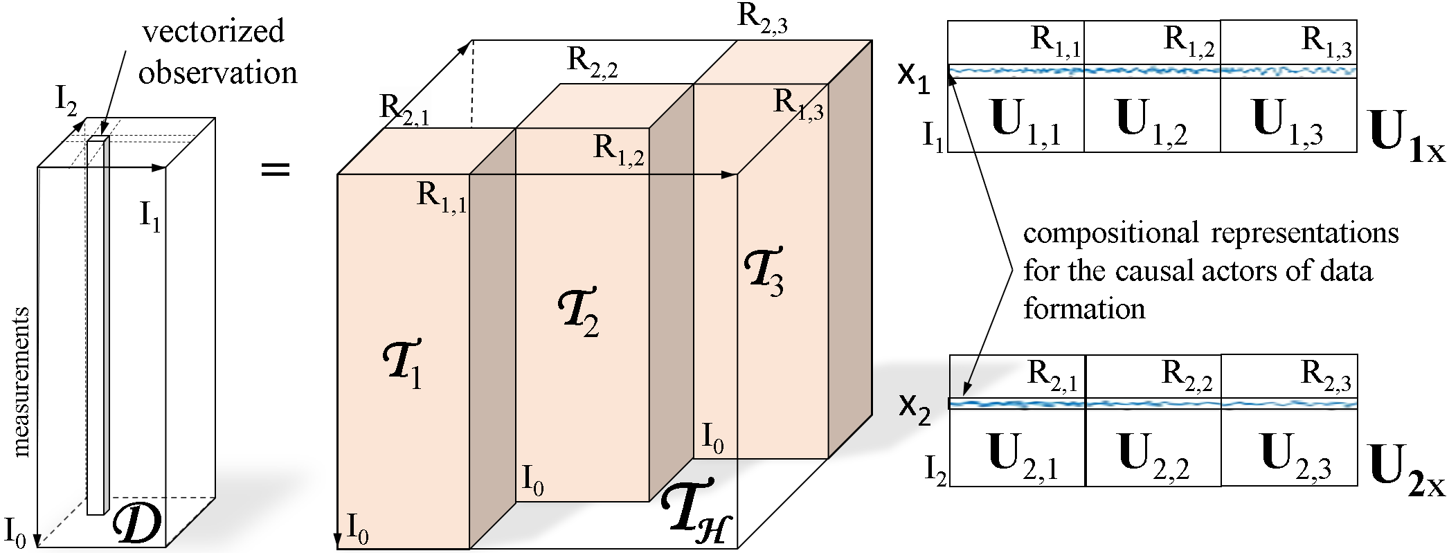
                                            (d) (e)

Figure 3. Compositional Hierarchical Tensor Factorization.(a) The data tensor, ${\mathbf{\mathcal{D}}}$, is rewriten in terms of a compositional hierarchical data tensor, ${\mathbf{\mathcal{D}}}_{\mbox{\tiny${\mathbf{\mathcal{H}}}$}}$. A fully compositional hierarchical data tensor is a data tensor in which every mode is written in a compositional form. The compositional hierarchical data tensor, ${\mathbf{\mathcal{D}}}_{\mbox{\tiny${\mathbf{\mathcal{H}}}$}}$, contains data tensor segments along its super-diagonal. The data tensor segment, ${\mathbf{\mathcal{D}}}_{s}$, may contain zeros and represent parts, or may be full and correspond to a filtered version of a parent-whole. (b) Only one of the causal factor has a compositional hierarchical representation, a partially compositional hierarchical representation example.(c) In practice, the measurement mode will not be written in a compositional form, ie. ${\mathbf{\mathcal{D}}}_{\mbox{\tiny${\mathbf{\mathcal{H}}}$}}$ would have already been multiplied with ${\textbf{I}}_{\mbox{\tiny{0}}}{}_{\mbox{\tiny{x}}}$as in Fig. 3(c1). (c1) Rewriting the data tensor ${\mathbf{\mathcal{D}}}$ as a hierarchical data tensor, ${\mathbf{\mathcal{D}}}_{\mbox{\tiny${\mathbf{\mathcal{H}}}$}}$. (c2) Performing a compositional hierarchical tensor factorization results in a part-based causal factor representation, ${\mathbf{\mathcal{D}}}={\mathbf{\mathcal{T}}}{{}_{\mbox{\tiny${\mathbf{\mathcal{H}}}$}}}\times_{\mbox{\tiny{1}}}{\textbf{U}}_{\mbox{\tiny{1x}}}\times_{\mbox{\tiny{2}}}{\textbf{U}}_{\mbox{\tiny{2x}}}$, where the extended core is ${\mathbf{\mathcal{T}}}_{\mbox{\tiny${\mathbf{\mathcal{H}}}$}}={\mathbf{\mathcal{Z}}}_{\mbox{\tiny${\mathbf{\mathcal{H}}}$}}\times_{\mbox{\tiny{0}}}{\textbf{U}}_{\mbox{\tiny{0}}}{}_{\mbox{\tiny{x}}}$.(d) Non-overlapping parts. The part representations’ computations are independent of one another. (e) Completely overlapping parts.

4. Compositional Hierarchical Tensor Factorizations

In prior tensor based research, an imaged object was represented in terms of global causal factor representations that are not robust to occlusions. This section introduces a compositional hierarchical tensor factorization that derives its name from its ability to represent a hierarchy of intrinsic and extrinsic causal factors of data formation.A hierarchical representation may be effectively employed to recognize occluded objects, including self-occlusion that occurs during out-of-plane rotation relative to the camera viewpoint. The efficacy of our approach is demonstrated by our LFW and Freiburg verification experiments that compare global and hierarchical representations in Section 5.

Within the tensor mathematical framework, an ensemble of training observations is organized in a higher order data tensor, ${\mathbf{\mathcal{D}}}$. A data tensor ${\mathbf{\mathcal{D}}}\in\mathbb{R}^{I_{\mbox{\tiny{0}}}\times I_{\mbox{\tiny{1}}}\times I_{\mbox{\tiny{c}}}\dots\times I_{\mbox{\tiny{C}}}}$ contains a collection of vectorized observation, ${\mathbf{d}}_{i_{\mbox{\tiny{1}}}\dots i_{\mbox{\tiny{c}}}\dots i_{\mbox{\tiny{C}}}}\in\mathbb{R}^{I_{\mbox{\tiny{0}}}}$ where each subscript, $i_{c}$, denotes one of the $C$ causal factors that have created the observation and have resulted in $I_{0}$ measurements, i.e., a total of $I_{\mbox{\tiny{0}}}$ pixels per image. In this paper, we will report results based on a data tensor ${\mathbf{\mathcal{D}}}$ of labeled, vectorized training facial images ${\mathbf{d}}_{pvle}$, where the subscripts denote the causal factors of facial image formation, the person $p$, view $v$, illumination $l$, and expression $e$ labels.

4.1. Hierarchical Data Tensor

We identify a general base case object and two special cases whose intrinsic and extrinsic causal factors we would like to represent. An object may be composed of (i) two partially overlapping children-parts and parent-whole that has data not contained in any of the children-parts, (ii) a set of non-overlapping parts, or (iii) a set of fully overlapping parts, which resembles to the rank-$(L,M,N)$ or a rank-$(L,M,\cdot)$ block tensor decomposition (DeLathauwer08, ), but which is too restrictive for our purpose. Figure 3 depicts the general base case and the two special base cases. In real scenarios, parent-wholes have children-parts that are recursively composed of children themselves, Fig. 4.

The data wholes, and parts are extracted by employing a filter bank, $\{{\textbf{H}}_{\mbox{\tiny{s}}}\|{\textbf{H}}_{\mbox{\tiny{s}}}\in\mathbb{C}^{J_{\mbox{\tiny{0}}}\times I_{\mbox{\tiny{0}}}},1\leq s\leq S\}$ where each $2D$ convolutional filter is implemented as a doubly (triply) block circulant matrix,${\textbf{H}}_{\mbox{\tiny{s}}}$, where $\sum_{s=1}^{S}{\textbf{H}}_{\mbox{\tiny{s}}}={\textbf{I}}$, and $s$ refers to the data segment. Convolution is a matrix-vector multiplication, between a circulant matrix and a vectorized observation, ${\mathbf{d}}_{\mbox{\tiny{s}}}={\textbf{H}}_{\mbox{\tiny{s}}}{\mathbf{d}}$ which in tensor notation is written as ${\mathbf{d}}_{\mbox{\tiny{s}}}={\mathbf{d}}\times_{\mbox{\tiny{0}}}{\textbf{H}}_{\mbox{\tiny{s}}}$ where mode $0$ is the measurement mode. The segment data tensor, ${\mathbf{\mathcal{D}}}_{s}={\mathbf{\mathcal{D}}}\times_{\mbox{\tiny{0}}}{\textbf{H}}_{\mbox{\tiny{s}}}$, is the result of multiplying (convolving) every observation, ${\mathbf{d}}$, with the block circulant matrix (filter), ${\textbf{H}}_{\mbox{\tiny{s}}}$. A filter ${\textbf{H}}_{\mbox{\tiny{s}}}$ may be any of any type, or have any spatial scope. When a filter matrix is a block identity matrix, ${\textbf{H}}_{\mbox{\tiny{s}}}={\textbf{I}}_{\mbox{\tiny{s}}}$, the filter matrix multiplication with a vectorized observation has the effect of segmenting a portion of the data without any blurring, subsampling or upsampling.Measurements associated with perceptual parts may may not be tightly packed into a block a priori, as in the case of vectorized images, but chunking may be achieved by a trivial permutation.

The data tensor, ${\mathbf{\mathcal{D}}}$, is expressed in terms of its recursive hierarchy of wholes and parts by defining and employing a hierarchical data tensor, ${\mathbf{\mathcal{D}}}_{\mbox{\tiny${\mathbf{\mathcal{H}}}$}}$, that contains along its super-diagonal the collection of wholes and parts, ${\mathbf{\mathcal{D}}}_{\mbox{\tiny{s}}}$, Fig. 3(a)

(7) $${\mathbf{\mathcal{D}}} = \sum_{s=1}^{S}{\mathbf{\mathcal{D}}}\times_{\mbox{\tiny{0}}}{\textbf{H}}_{\mbox{\tiny{s}}}$$

(8) $$= {\mathbf{\mathcal{D}}}_{\mbox{\tiny{1}}}\dots+{\mathbf{\mathcal{D}}}_{\mbox{\tiny{s}}}\dots+{\mathbf{\mathcal{D}}}_{\mbox{\tiny{S}}}$$

(9) $$= {\mathbf{\mathcal{D}}}{{}_{\mbox{\tiny${\mathbf{\mathcal{H}}}$}}}\times_{\mbox{\tiny{0}}}{\textbf{I}}_{\mbox{\tiny{Ox}}}\times_{\mbox{\tiny{1}}}{\textbf{I}}_{\mbox{\tiny{1x}}}\dots\times_{\mbox{\tiny{c}}}{\textbf{I}}_{\mbox{\tiny{cx}}}\dots\times_{\mbox{\tiny{C}}}{\textbf{I}}_{\mbox{\tiny{Cx}}},\vspace{-.35in}$$

where ${\textbf{I}}_{\mbox{\tiny{cx}}}=[{\textbf{I}}_{\mbox{\tiny{c,1}}}...{\textbf{I}}_{\mbox{\tiny{c,s}}}...{\textbf{I}}_{\mbox{\tiny{c,S}}}]\in\mathbb{R}^{I_{c}\times SI_{c}}$ is a concatenation of $S$ identity matrices, one for each data segment. The three different ways of rewritting ${\mathbf{\mathcal{D}}}$ in terms of a hierarchy of wholes and parts, eq. 7-9, results in three equivalent compositional hierarchical tensor factorizations 

(10) $$\hskip-57.81621pt{\mathbf{\mathcal{D}}} \hskip-7.22743pt= \hskip-7.22743pt\sum_{s=1}^{S}\underbrace{({\mathbf{\mathcal{Z}}}\times_{\mbox{\tiny{0}}}{\textbf{U}}_{\mbox{\tiny{0}}}\times_{\mbox{\tiny{1}}}{\textbf{U}}_{\mbox{\tiny{1}}}\dots\times_{\mbox{\tiny{c}}}{\textbf{U}}_{\mbox{\tiny{c}}}\dots\times_{\mbox{\tiny{C}}}{\textbf{U}}_{\mbox{\tiny{C}}})}_{\mbox{${\mathbf{\mathcal{D}}}$}}\times_{\mbox{\tiny{0}}}{\textbf{H}}_{\mbox{\tiny{s}}}$$

(12) $$\hskip-7.22743pt= \hskip-7.22743pt\sum_{s=1}^{S}\underbrace{({\mathbf{\mathcal{Z}}}_{\mbox{\tiny{s}}}\times_{\mbox{\tiny{0}}}{\textbf{U}}_{\mbox{\tiny{0}}}{}_{\mbox{\tiny{,s}}}\times_{\mbox{\tiny{1}}}{\textbf{U}}_{\mbox{\tiny{1,s}}}\dots\times_{\mbox{\tiny{c}}}{\textbf{U}}_{\mbox{\tiny{c,s}}}\dots\times_{\mbox{\tiny{C}}}{\textbf{U}}_{\mbox{\tiny{C,s}}})}_{\mbox{${\mathbf{\mathcal{D}}}_{\mbox{\tiny{s}}}$}}$$

$$\hskip-7.22743pt= \hskip-7.22743pt\underbrace{({\mathbf{\mathcal{Z}}}_{\mbox{\tiny${\mathbf{\mathcal{H}}}$}}\times_{\mbox{\tiny{0}}}{\textbf{U}}_{\mbox{\tiny{0}}}{}_{\mbox{\tiny${\mathbf{\mathcal{H}}}$}}\times_{\mbox{\tiny{1}}}{\textbf{U}}_{\mbox{\tiny{1}}}{}_{\mbox{\tiny${\mathbf{\mathcal{H}}}$}}\dots\times_{\mbox{\tiny{c}}}{\textbf{U}}_{\mbox{\tiny{c}}}{}_{\mbox{\tiny${\mathbf{\mathcal{H}}}$}}\dots\times_{\mbox{\tiny{C}}}{\textbf{U}}_{\mbox{\tiny{C}}}{}_{\mbox{\tiny${\mathbf{\mathcal{H}}}$}})}_{\mbox{${\mathbf{\mathcal{D}}}_{\mbox{\tiny${\mathbf{\mathcal{H}}}$}}$}}$$

$$\hskip 14.45377pt\times_{\mbox{\tiny{0}}}{\textbf{I}}_{\mbox{\tiny{0x}}}\times_{\mbox{\tiny{1}}}{\textbf{I}}_{\mbox{\tiny{1x}}}\dots\times_{\mbox{\tiny{c}}}{\textbf{I}}_{\mbox{\tiny{cx}}}\dots\times_{\mbox{\tiny{C}}}{\textbf{I}}_{\mbox{\tiny{Cx}}}$$

The expression of ${\mathbf{\mathcal{D}}}$ in terms of a hierarchical data tensor is a mathematical conceptual device, that enables a unified mathematical model of wholes and parts that can be expressed completely as a mode-m product (matrix-vector multiplication) and whose factorization can be optimized in a principled manner. Dimensionality reduction of the compositional representation is performed by optimizing

(13) $$\hskip-28.90755pte \hskip-18.06749pt=\hskip-9.03374pt=\frac{1}{2}\|{\mathbf{\mathcal{D}}}\hskip-1.8063pt-\hskip-1.8063pt(\hskip 1.8063pt\bar{{\mathbf{\mathcal{Z}}}}_{\mbox{\tiny${\mathbf{\mathcal{H}}}$}}\times_{\mbox{\tiny{0}}}\bar{{\textbf{U}}}_{\mbox{\tiny{0}}}{}_{\mbox{\tiny${\mathbf{\mathcal{H}}}$}}...\times_{\mbox{\tiny{c}}}\bar{{\textbf{U}}}_{\mbox{\tiny{c}}}{}_{\mbox{\tiny${\mathbf{\mathcal{H}}}$}}...\times_{\mbox{\tiny{C}}}\bar{{\textbf{U}}}_{\mbox{\tiny{C}}}{}_{\mbox{\tiny${\mathbf{\mathcal{H}}}$}})$$

$$\hskip 14.45377pt\times_{\mbox{\tiny{0}}}{\textbf{I}}_{\mbox{\tiny{0x}}}...\times_{\mbox{\tiny{c}}}{\textbf{I}}_{\mbox{\tiny{cx}}}...\times_{\mbox{\tiny{C}}}{\textbf{I}}_{\mbox{\tiny{Cx}}}\|^{2}+\sum_{c=0}^{C}\lambda_{\mbox{\tiny{c}}}\|{{\bar{{\textbf{U}}}_{\mbox{\tiny{c}}}}{}^{\mathrm{T}}_{\mbox{\tiny${\mathbf{\mathcal{H}}}$}}}{\bar{{\textbf{U}}}_{\mbox{\tiny{c}}}}{}_{\mbox{\tiny${\mathbf{\mathcal{H}}}$}}-{\textbf{I}}\|^{2}\vspace{-.5in}$$

where $\bar{{\textbf{U}}}_{\mbox{\tiny{c}}}{}_{\mbox{\tiny${\mathbf{\mathcal{H}}}$}}$ is the composite representation of the $c^{\mbox{\small th}}$ mode, and ${\mathbf{\mathcal{Z}}}_{\mbox{\tiny${\mathbf{\mathcal{H}}}$}}$ governs the interaction between causal factors. Our optimization may be initialized, only, by setting ${\mathbf{\mathcal{Z}}}_{\mbox{\tiny${\mathbf{\mathcal{H}}}$}}$ and ${\textbf{U}}_{\mbox{\tiny{c}}}{}_{\mbox{\tiny${\mathbf{\mathcal{H}}}$}}$ to the M-mode SVD of ${\mathbf{\mathcal{D}}}_{\mbox{\tiny${\mathbf{\mathcal{H}}}$}}$, and performing dimensionality reduction through truncation, where $\bar{{\textbf{U}}}_{\mbox{\tiny{c}}}{}_{\mbox{\tiny${\mathbf{\mathcal{H}}}$}}\in\mathbb{R}^{SI_{c}\times\bar{J}_{c}}$, $\bar{{\mathbf{\mathcal{Z}}}}_{\mbox{\tiny${\mathbf{\mathcal{H}}}$}}\in\mathbb{R}^{\bar{J}_{0}\dots\times\bar{J}_{c}\dots\times\bar{J}_{C}}$ and $\bar{J}_{\mbox{\tiny{c}}}\leq SI_{\mbox{\tiny{c}}}$.

4.2. Compositional Hierarchical Factorization Derivation

For notational simplicity, we re-write the loss function as,

(14) $$e\hskip-7.22743pt \mathrel{\mathop{:}}= \hskip-7.22743pt\frac{1}{2}\|{\mathbf{\mathcal{D}}}-\tilde{{\mathbf{\mathcal{Z}}}}{{}_{\mbox{\tiny${\mathbf{\mathcal{H}}}$}}}\times_{\mbox{\tiny{0}}}\tilde{{\textbf{U}}}_{\mbox{\tiny{0x}}}...\times_{\mbox{\tiny{c}}}\tilde{{\textbf{U}}}_{\mbox{\tiny{cx}}}...\times_{\mbox{\tiny{C}}}\tilde{{\textbf{U}}}_{\mbox{\tiny{Cx}}}\|^{2}$$

$$\hskip-7.22743pt+\sum_{c=0}^{C}\sum_{s=1}^{S}\lambda_{\mbox{\tiny{c,s}}}\|\tilde{{\textbf{U}}}_{\mbox{\tiny{c,s}}}^{\mathrm{T}}\tilde{{\textbf{U}}}_{\mbox{\tiny{c,s}}}-{\textbf{I}}\|\vspace{-.5in}$$

where $\tilde{{\textbf{U}}}_{\mbox{\tiny{cx}}}={\textbf{I}}_{\mbox{\tiny{cx}}}\bar{{\textbf{U}}}_{\mbox{\tiny{c}}}{}_{\mbox{\tiny${\mathbf{\mathcal{H}}}$}}\tilde{{\textbf{G}}}_{\mbox{\tiny{c}}}=[\tilde{{\textbf{U}}}_{\mbox{\tiny{c,1}}}|\dots|\tilde{{\textbf{U}}}_{\mbox{\tiny{c,s}}}|\dots|\tilde{{\textbf{U}}}_{\mbox{\tiny{c,S}}}]$ and $\tilde{{\textbf{G}}}_{\mbox{\tiny{c}}}\in\mathbb{R}^{\bar{J}_{c}\times SI_{c}}$ is permutation matrix that groups the columns of ${\textbf{U}}_{\mbox{\tiny{c}}}{}_{\mbox{\tiny${\mathbf{\mathcal{H}}}$}}$ based on the segment, $s$, to which they belong, and the inverse permutation matrices have been multiplied${}^{\ref{note:equivalence}}$ into $\tilde{{\mathbf{\mathcal{Z}}}}_{\mbox{\tiny${\mathbf{\mathcal{H}}}$}}$ resulting into a core that has also been grouped based on segments and sorted based on variance. The data tensor, ${\mathbf{\mathcal{D}}}$, may be expressed in matrix form as in eq. 16 and reduces to the more efficiently block structure as in eq. 4.2

(15) $$\hskip-18.06749pt{{\mathbf{\mathcal{D}}}} \hskip-10.84006pt={{\mathbf{\mathcal{Z}}}}_{\mbox{\tiny${\mathbf{\mathcal{H}}}$}}\times_{\mbox{\tiny{0}}}{{\textbf{U}}}_{\mbox{\tiny{0x}}}\times_{\mbox{\tiny{1}}}{{\textbf{U}}}_{\mbox{\tiny{1x}}}\dots\times_{\mbox{\tiny{c}}}{{\textbf{U}}}_{\mbox{\tiny{cx}}}\dots\times_{\mbox{\tiny{C}}}{{\textbf{U}}}_{\mbox{\tiny{Cx}}}$$

(16) $$\hskip-10.84006pt{{\textbf{D}}}_{\mbox{\tiny{[c]}}} \hskip-10.84006pt={{\textbf{U}}}_{\mbox{\tiny{cx}}}{{\textbf{Z}}}_{\mbox{\tiny${\mathbf{\mathcal{H}}}$}}{}_{\mbox{\tiny{[c]}}}\left({{\textbf{U}}}_{\mbox{\tiny{Cx}}}\otimes\dots\otimes{{\textbf{U}}}_{\mbox{\tiny{(c+1)x}}}\otimes{{\textbf{U}}}_{\mbox{\tiny{(c-1)x}}}\otimes\dots\otimes{{\textbf{U}}}_{\mbox{\tiny{0x}}}\right)^{\mathrm{T}}\hskip-21.68121pt$$

$$\hskip-10.84006pt= \hskip-10.84006pt\left[\hskip 1.8063pt{{\textbf{U}}}_{\mbox{\tiny{c,1}}}\dots{\textbf{U}}_{\mbox{\tiny{c,s}}}\dots{\textbf{U}}_{\mbox{\tiny{c,S}}}\hskip 1.8063pt\right]\hskip-21.68121pt$$

$$\hskip-10.84006pt\left[\hskip-3.97432pt\begin{array}[]{ccccc}{{\textbf{Z}}}_{\mbox{\tiny{0[c]}}}&\hskip-7.22743pt{\textbf{0}}&\hskip-7.22743pt&\hskip-7.22743pt\cdots&\hskip-7.22743pt{\textbf{0}}\\ {\textbf{0}}&\hskip-7.22743pt\ddots&\hskip-7.22743pt{\textbf{0}}&\hskip-7.22743pt&\hskip-7.22743pt\vdots\\ \vdots&\hskip-7.22743pt{\textbf{0}}&\hskip-7.22743pt{{\textbf{Z}}}_{\mbox{\tiny{s[c]}}}&\hskip-7.22743pt{\textbf{0}}&\hskip-7.22743pt\\ &\hskip-7.22743pt&\hskip-7.22743pt{\textbf{0}}&\hskip-7.22743pt\ddots&\hskip-7.22743pt{\textbf{0}}\\ {\textbf{0}}&\hskip-7.22743pt\cdots&\hskip-7.22743pt&\hskip-7.22743pt{\textbf{0}}&\hskip-7.22743pt{{\textbf{Z}}}_{\mbox{\tiny{S[c]}}}\end{array}\hskip-5.42003pt\right]\hskip-1.8063pt\underbrace{\left[\hskip-3.61371pt\begin{array}[]{c}\left({{\textbf{U}}}_{\mbox{\tiny{C,1}}}...\otimes{{\textbf{U}}}_{\mbox{\tiny{(c+1),1}}}\otimes{{\textbf{U}}}_{\mbox{\tiny{(c-1),1}}}...\otimes{{\textbf{U}}}_{\mbox{\tiny{0,1}}}\right)^{\mathrm{T}}\\ \vdots\\ \left({{\textbf{U}}}_{\mbox{\tiny{C,s}}}...\otimes{{\textbf{U}}}_{\mbox{\tiny{(c+1),s}}}\otimes{{\textbf{U}}}_{\mbox{\tiny{(c-1),s}}}...\otimes{{\textbf{U}}}_{\mbox{\tiny{0,s}}}\right)^{\mathrm{T}}\\ \vdots\\ \left({{\textbf{U}}}_{\mbox{\tiny{C,S}}}...\otimes{{\textbf{U}}}_{\mbox{\tiny{(c+1),S}}}\otimes{{\textbf{U}}}_{\mbox{\tiny{(c-1),S}}}...\otimes{{\textbf{U}}}_{\mbox{\tiny{0,S}}}\right)^{\mathrm{T}}\\ \end{array}\hskip-5.42003pt\right]}\hskip-5.42003pt$$

$$\hskip 79.49744pt{\left({{\textbf{U}}}_{\mbox{\tiny{Cx}}}\dots\odot{{\textbf{U}}}_{\mbox{\tiny{(c+1)x}}}\odot{{\textbf{U}}}_{\mbox{\tiny{(c-1)x}}}\dots\odot{{\textbf{U}}}_{\mbox{\tiny{0x}}}\right)^{\mathrm{T}}}$$

(29) $$\hskip-7.22743pt={{\textbf{U}}}_{\mbox{\tiny{cx}}}{\textbf{W}}_{\mbox{\tiny{c}}}^{\mathrm{T}},\hskip-25.29494pt\vspace{-.5in}$$

where $\otimes$ is the Kronecker product,and $\odot$ is the block-matrix Kahtri-Rao product. The matricized block diagonal form of ${{\mathbf{\mathcal{Z}}}}_{\mbox{\tiny${\mathbf{\mathcal{H}}}$}}$ in eq. 4.2 becomes evident when employing our modified data centric matrixizing operator based on the defintion 1, where the initial mode is the measurement mode.

The compositional hierarchical tensor factorization algorithm computes the mode matrix, ${{\textbf{U}}}_{\mbox{\tiny{cx}}}$, by computing the minimum of $e=\|{\mathbf{\mathcal{D}}}-\tilde{{\mathbf{\mathcal{Z}}}}_{\mbox{\tiny${\mathbf{\mathcal{H}}}$}}\times_{\mbox{\tiny{0}}}\tilde{{\textbf{U}}}_{\mbox{\tiny{0x}}}\dots\times_{\mbox{\tiny{C}}}\tilde{{\textbf{U}}}_{\mbox{\tiny{Cx}}}\|^{2}$ by cycling through the modes, solving for $\tilde{{\textbf{U}}}_{\mbox{\tiny{cx}}}$ in the equation $\partial e/\partial{\textbf{U}}_{\mbox{\tiny{cx}}}=0$ while holding the core tensor ${\mathbf{\mathcal{Z}}}_{\mbox{\tiny${\mathbf{\mathcal{H}}}$}}$ and all the other mode matrices constant, and repeating until convergence. Note that

(30) $${\partial e\over\partial{\textbf{U}}_{\mbox{\tiny{cx}}}}\hskip-1.8063pt=\hskip-1.8063pt{\partial\over\partial{\textbf{U}}_{\mbox{\tiny{cx}}}}\|{{{\textbf{D}}}_{\mbox{\tiny{$[c]$}}}}-{\textbf{U}}_{\mbox{\tiny{cx}}}{\textbf{W}}_{\mbox{\tiny{c}}}^{\mathrm{T}}\|^{2}\hskip-1.8063pt=-{{{\textbf{D}}}_{\mbox{\tiny{$[c]$}}}}{\textbf{W}}_{\mbox{\tiny{c}}}+{\textbf{U}}_{\mbox{\tiny{cx}}}{\textbf{W}}_{\mbox{\tiny{c}}}^{\mathrm{T}}{\textbf{W}}_{\mbox{\tiny{c}}}.$$

Thus, $\partial e/\partial{\textbf{U}}_{\mbox{\tiny{c}}}{}_{\mbox{\tiny{x}}}=0$ implies that

(31) $$\hskip-21.68121pt{\textbf{U}}_{\mbox{\tiny{cx}}}= \hskip-3.61371pt{{{\textbf{D}}}_{\mbox{\tiny{$[c]$}}}}{\textbf{W}}_{\mbox{\tiny{c}}}\left({\textbf{W}}_{\mbox{\tiny{c}}}^{\mathrm{T}}{\textbf{W}}_{\mbox{\tiny{c}}}\right)^{-1}={{{\textbf{D}}}_{\mbox{\tiny{$[c]$}}}}{\textbf{W}}_{\mbox{\tiny{c}}}^{\mathrm{T}}{}^{+\lower 2.0pt\hbox{\hskip-2.0pt\hbox{\tiny${}$}}}\hskip-54.2025pt$$

(32) $$\hskip-36.135pt= \hskip-20.59721pt{{{\textbf{D}}}_{\mbox{\tiny{$[c]$}}}}\left({\textbf{Z}}_{\mbox{\tiny${\mathbf{\mathcal{H}}}$}}{}_{\mbox{\tiny{[c]}}}\left({{\textbf{U}}}_{\mbox{\tiny{Cx}}}\otimes...{{\textbf{U}}}_{\mbox{\tiny{(c+1)x}}}\otimes{{\textbf{U}}}_{\mbox{\tiny{(c-1)x}}}\otimes...{{\textbf{U}}}_{\mbox{\tiny{0x}}}\right)^{\mathrm{T}}\right)^{+\lower 2.0pt\hbox{\hskip-2.0pt\hbox{\tiny${}$}}}\hskip-54.2025pt$$

(38) $$\hskip-36.135pt= \hskip-20.59721pt{{{\textbf{D}}}_{\mbox{\tiny{$[c]$}}}}\hskip-1.8063pt\left({{\textbf{U}}}_{\mbox{\tiny{Cx}}}\hskip-3.61371pt\odot...{{\textbf{U}}}_{\mbox{\tiny{(c+1)x}}}\hskip-1.8063pt\odot\hskip-1.8063pt{{\textbf{U}}}_{\mbox{\tiny{(c-1)x}}}\hskip-1.8063pt\odot...{{\textbf{U}}}_{\mbox{\tiny{0x}}}\right)\hskip-3.61371pt^{\mathrm{T}}{}^{+\lower 2.0pt\hbox{\hskip-2.0pt\hbox{\tiny${}$}}}\hskip-1.8063pt\left[\hskip-5.42003pt\begin{array}[]{ccccc}{{\textbf{Z}}}_{\mbox{\tiny{0[c]}}}^{+\lower 2.0pt\hbox{\hskip-2.0pt\hbox{\tiny${}$}}}&\hskip-7.22743pt{\textbf{0}}&\hskip-7.22743pt&\hskip-7.22743pt\cdots&\hskip-7.22743pt{\textbf{0}}\\ {\textbf{0}}&\hskip-7.22743pt\ddots&\hskip-7.22743pt{\textbf{0}}&\hskip-7.22743pt&\hskip-7.22743pt\vdots\\ \vdots&\hskip-7.22743pt{\textbf{0}}&\hskip-7.22743pt{{\textbf{Z}}}_{\mbox{\tiny{s[c]}}}^{+\lower 2.0pt\hbox{\hskip-2.0pt\hbox{\tiny${}$}}}&\hskip-7.22743pt{\textbf{0}}&\hskip-7.22743pt\\ &\hskip-7.22743pt&\hskip-7.22743pt{\textbf{0}}&\hskip-7.22743pt\ddots&\hskip-7.22743pt{\textbf{0}}\\ {\textbf{0}}&\hskip-7.22743pt\cdots&\hskip-7.22743pt&\hskip-7.22743pt{\textbf{0}}&\hskip-7.22743pt{{\textbf{Z}}}_{\mbox{\tiny{S[c]}}}^{+\lower 2.0pt\hbox{\hskip-2.0pt\hbox{\tiny${}$}}}\end{array}\hskip-5.42003pt\right]$$

whose ${\textbf{U}}_{\mbox{\tiny{c,s}}}$ sub-matrices are then subject to orthonormality constraints.

Solving for the optimal core tensor, ${\mathbf{\mathcal{Z}}}_{\mbox{\tiny${\mathbf{\mathcal{H}}}$}}$, the data tensor, ${\mathbf{\mathcal{D}}}$, approximation is expressed in vector form as,

(39) $$e=\|\mathrm{vec}({{\mathbf{\mathcal{D}}}})-(\tilde{{\textbf{U}}}_{\mbox{\tiny{Cx}}}\otimes\dots\otimes\tilde{{\textbf{U}}}_{\mbox{\tiny{cx}}}\otimes\dots\otimes\tilde{{\textbf{U}}}_{\mbox{\tiny{0x}}})\mathrm{vec}(\tilde{{\mathbf{\mathcal{Z}}}}_{\mbox{\tiny${\mathbf{\mathcal{H}}}$}})\|.\vspace{-.1in}$$

Solve for the non-zero(nz) terms of ${\mathbf{\mathcal{Z}}}_{\mbox{\tiny${\mathbf{\mathcal{H}}}$}}$ in the equation $\partial e/\partial({\small{\mathbf{\mathcal{Z}}}_{\mbox{\tiny${\mathbf{\mathcal{H}}}$}}})=0$, by removing the corresponding zero columns of the first matrix on right side of the equation below, performing the pseudo-inverse, and setting

(40) $$\mathrm{vec}({\mathbf{\mathcal{Z}}}_{\mbox{\tiny${\mathbf{\mathcal{H}}}$}})_{\mbox{\tiny{nz}}}=({\textbf{U}}_{\mbox{\tiny{Cx}}}\otimes\dots\otimes{\textbf{U}}_{\mbox{\tiny{cx}}}\otimes\dots\otimes{\textbf{U}}_{\mbox{\tiny{0x}}})^{+\lower 2.0pt\hbox{\hskip-2.0pt\hbox{\tiny${}$}}}_{\mbox{\tiny{nz}}}\mathrm{vec}({\mathbf{\mathcal{D}}}).\vspace{-.05in}$$

Input: Data tensor, ${\mathbf{\mathcal{D}}}\in\mathbb{R}^{I_{\mbox{\tiny{0}}}\times I_{\mbox{\tiny{1}}}\times\dots\times I_{\mbox{\tiny{C}}}}$, filters ${\textbf{H}}_{\mbox{\tiny{s}}}$, and desired dimensionality reduction $\tilde{J}_{\mbox{\tiny{1}}},\dots,\tilde{J}_{\mbox{\tiny{C}}}$.

1. 1.Initialization:

2. Decompose each data tensor segment, ${\mathbf{\mathcal{D}}}_{\mbox{\tiny{s}}}={\mathbf{\mathcal{D}}}\times{\textbf{H}}_{\mbox{\tiny{s}}}$, by employing the M-mode SVD.

   $${\mathbf{\mathcal{D}}}_{\mbox{\tiny{s}}}={\mathbf{\mathcal{Z}}}\times_{\mbox{\tiny{0}}}{\textbf{U}}_{\mbox{\tiny{0}}}{}_{\mbox{\tiny{,s}}}\dots\times_{\mbox{\tiny{c}}}{\textbf{U}}_{\mbox{\tiny{c,s}}}\dots\times_{\mbox{\tiny{C}}}{\textbf{U}}_{\mbox{\tiny{C,s}}}$$

3. For $c=0,1,\dots,C$, set ${\textbf{U}}_{\mbox{\tiny{cx}}}=[{\textbf{U}}_{\mbox{\tiny{c,1}}}...{\textbf{U}}_{\mbox{\tiny{c,s}}}...{\textbf{U}}_{\mbox{\tiny{c,S}}}]$, and truncate to $\tilde{J}_{\mbox{\tiny{c}}}$ columns by sorting all the eigenvalues from all data segments and deleting the columns corresponding to the lowest eigenvalues from various ${\textbf{U}}_{\mbox{\tiny{c,s}}}$ and the rows from ${\textbf{Z}}_{\mbox{\tiny{s[c]}}}$

4. 2.Optimization via alternating least squares:
   

5. Iterate for $n\mathrel{\mathop{:}}=1,\dots,N$

   • For $c\mathrel{\mathop{:}}=0,\dots,C$,

   • 2a. Compute mode matrix ${\textbf{U}}_{\mbox{\tiny{cx}}}$ while holding the rest fixed.

     $$\hskip 18.06749pt{\textbf{U}}_{\mbox{\tiny{cx}}} \hskip-10.84006pt\mathrel{\mathop{:}}=\hskip-9.03374pt {{{\textbf{D}}}_{\mbox{\tiny{$[c]$}}}}\hskip-3.97432pt\left({{\textbf{U}}}_{\mbox{\tiny{Cx}}}\hskip-3.61371pt\odot...{{\textbf{U}}}_{\mbox{\tiny{(c+1)x}}}\hskip-1.8063pt\odot\hskip-1.8063pt{{\textbf{U}}}_{\mbox{\tiny{(c-1)x}}}\hskip-1.8063pt\odot...{{\textbf{U}}}_{\mbox{\tiny{0x}}}\right)\hskip-3.97432pt^{\mathrm{T}}{\hskip-1.8063pt}^{+\lower 2.0pt\hbox{\hskip-2.0pt\hbox{\tiny${}$}}}\hskip-1.8063pt\left[\hskip-5.42003pt\begin{array}[]{ccccc}{{\textbf{Z}}}_{\mbox{\tiny{0[c]}}}^{+\lower 2.0pt\hbox{\hskip-2.0pt\hbox{\tiny${}$}}}&\hskip-7.22743pt{\textbf{0}}&\hskip-7.22743pt&\hskip-7.22743pt\cdots&\hskip-7.22743pt{\textbf{0}}\\ {\textbf{0}}&\hskip-7.22743pt\ddots&\hskip-7.22743pt{\textbf{0}}&\hskip-7.22743pt&\hskip-7.22743pt\vdots\\ \vdots&\hskip-7.22743pt{\textbf{0}}&\hskip-7.22743pt{{\textbf{Z}}}_{\mbox{\tiny{s[c]}}}^{+\lower 2.0pt\hbox{\hskip-2.0pt\hbox{\tiny${}$}}}&\hskip-7.22743pt{\textbf{0}}&\hskip-7.22743pt\\ &\hskip-7.22743pt&\hskip-7.22743pt{\textbf{0}}&\hskip-7.22743pt\ddots&\hskip-7.22743pt{\textbf{0}}\\ {\textbf{0}}&\hskip-7.22743pt\cdots&\hskip-7.22743pt&\hskip-7.22743pt{\textbf{0}}&\hskip-7.22743pt{{\textbf{Z}}}_{\mbox{\tiny{S[c]}}}^{+\lower 2.0pt\hbox{\hskip-2.0pt\hbox{\tiny${}$}}}\end{array}\hskip-5.42003pt\right]$$

   • Set $\hat{{\textbf{U}}}_{\mbox{\tiny{c,s}}}$ to the $\tilde{R}_{\mbox{\tiny{c,s}}}$ leading left-singular vectors of the SVD of

   • ${\textbf{U}}_{\mbox{\tiny{c,s}}}$, a subset of the columns in ${\textbf{U}}_{\mbox{\tiny{cx}}}$.Update ${\textbf{U}}_{\mbox{\tiny{c,s}}}$ in ${{\textbf{U}}}_{\mbox{\tiny{cx}}}$ with $\hat{{\textbf{U}}}_{\mbox{\tiny{c,s}}}$

   • 2b. Set the non-zero(nz) entries of $\mathrm{vec}({\mathbf{\mathcal{Z}}}_{\mbox{\tiny${\mathbf{\mathcal{H}}}$}})_{\mbox{\tiny{nz}}}$ based on:

     $$\hskip 21.68121pt\mathrm{vec}({\mathbf{\mathcal{Z}}}_{\mbox{\tiny${\mathbf{\mathcal{H}}}$}})_{\mbox{\tiny{nz}}}=({\textbf{U}}_{\mbox{\tiny{Cx}}}\otimes\dots\otimes{\textbf{U}}_{\mbox{\tiny{cx}}}\otimes\dots\otimes{\textbf{U}}_{\mbox{\tiny{0x}}})^{+\lower 2.0pt\hbox{\hskip-2.0pt\hbox{\tiny${}$}}}_{\mbox{\tiny{nz}}}\mathrm{vec}({\mathbf{\mathcal{D}}}).$$

   until convergence.  

Output converged matrices ${{\textbf{U}}}_{\mbox{\tiny{1x}}},\dots,{{\textbf{U}}}_{\mbox{\tiny{Cx}}}$ and tensor ${{\mathbf{\mathcal{Z}}}}{{}_{\mbox{\tiny${\mathbf{\mathcal{H}}}$}}}$.  

Algorithm 2 Compositional Hierarchical Tensor Factorization.

Repeat all steps until convergence.This optimization is the basis of the Compositional Hierarchical Tensor Factorization, Algorithm 2.

Completely Overlapping parts: When the data tensor is a collection of overlapping parts that have the same multilinear-rank reduction, Fig. 3e, the extended-core data tensor, ${\mathbf{\mathcal{T}}}_{\mbox{\tiny${\mathbf{\mathcal{H}}}$}}$, computation in matrix form reduces to eq. 59

(46) $$\hskip-39.74872pt{{\mathbf{\mathcal{D}}}} \hskip-3.61371pt= \hskip-3.61371pt{{\mathbf{\mathcal{T}}}}_{\mbox{\tiny${\mathbf{\mathcal{H}}}$}}\times_{\mbox{\tiny{1}}}{{\textbf{U}}}_{\mbox{\tiny{1x}}}\dots\times_{\mbox{\tiny{c}}}{{\textbf{U}}}_{\mbox{\tiny{cx}}}\dots\times_{\mbox{\tiny{C}}}{{\textbf{U}}}_{\mbox{\tiny{Cx}}}$$

(47) $$\vspace{+.2in}{{\textbf{D}}}_{\mbox{\tiny{[0]}}} \hskip-3.61371pt= \hskip-3.61371pt{{\textbf{T}}}_{\mbox{\tiny${\mathbf{\mathcal{H}}}$}}{}_{\mbox{\tiny{[0]}}}({{\textbf{U}}}_{\mbox{\tiny{Cx}}}\dots\otimes{{\textbf{U}}}_{\mbox{\tiny{cx}}}\dots\otimes{{\textbf{U}}}_{\mbox{\tiny{1x}}})^{\mathrm{T}}$$

(59) $$\vspace{-.1in}\left[\begin{array}[]{c}{{\textbf{T}}}_{\mbox{\tiny{1[0]}}}\\ \vdots\\ {{\textbf{T}}}_{\mbox{\tiny{s[0]}}}\\ \vdots\\ {{\textbf{T}}}_{\mbox{\tiny{S[0]}}}\end{array}\right]^{\mathrm{T}} \hskip-10.84006pt= \hskip-7.22743pt{{\textbf{D}}}_{\mbox{\tiny{[0]}}}\underbrace{\left[\begin{array}[]{c}({{\textbf{U}}}_{\mbox{\tiny{C,1}}}\dots\otimes{{\textbf{U}}}_{\mbox{\tiny{c,1}}}\dots\otimes{{\textbf{U}}}_{\mbox{\tiny{1,1}}})^{\mathrm{T}}\\ \vdots\\ ({{\textbf{U}}}_{\mbox{\tiny{C,s}}}\dots\otimes{{\textbf{U}}}_{\mbox{\tiny{c,s}}}\dots\otimes{{\textbf{U}}}_{\mbox{\tiny{1,s}}})^{\mathrm{T}}\\ \vdots\\ ({{\textbf{U}}}_{\mbox{\tiny{C,S}}}\dots\otimes{{\textbf{U}}}_{\mbox{\tiny{c,S}}}\dots\otimes{{\textbf{U}}}_{\mbox{\tiny{1,S}}})^{\mathrm{T}}\end{array}\right]^{+\lower 2.0pt\hbox{\hskip-2.0pt\hbox{\tiny${}$}}}}_{{\left(\begin{array}[]{c}{{\textbf{U}}}_{\mbox{\tiny{Cx}}}\cdots\odot{{\textbf{U}}}_{\mbox{\tiny{cx}}}\cdots\odot{{\textbf{U}}}_{\mbox{\tiny{1x}}}\end{array}\right)^{\mathrm{T}}}^{+\lower 2.0pt\hbox{\hskip-2.0pt\hbox{\tiny${}$}}}}.$$

Independent Parts: When the data tensor is a collection of observations made up of non-overlapping parts, Fig. 3d, the data tensor decomposition reduces to the concatenation of a $M$-mode SVD of individual parts,

(70) $$\hskip-14.45377pt\left[\begin{array}[]{c}{\textbf{D}}_{\mbox{\tiny{1[c]}}}\\ \vdots\\ {\textbf{D}}_{\mbox{\tiny{s[c]}}}\\ \vdots\\ {\textbf{D}}_{\mbox{\tiny{S[c]}}}\\ \end{array}\right] \hskip-5.42003pt= \hskip-5.42003pt\left[\hskip-3.61371pt\begin{array}[]{ccccc}{{\textbf{U}}}_{\mbox{\tiny{c,1}}}{\textbf{Z}}_{\mbox{\tiny{0[c]}}}({{\textbf{U}}}_{\mbox{\tiny{C,1}}}\dots\otimes{{\textbf{U}}}_{\mbox{\tiny{(c+1),1}}}\otimes{{\textbf{U}}}_{\mbox{\tiny{(c-1),1}}}\dots\otimes{{\textbf{U}}}_{\mbox{\tiny{0,1}}})^{\mathrm{T}}\\ \vdots\\ {{\textbf{U}}}_{\mbox{\tiny{c,s}}}{\textbf{Z}}_{\mbox{\tiny{s[c]}}}({{\textbf{U}}}_{\mbox{\tiny{C,s}}}\dots\otimes{{\textbf{U}}}_{\mbox{\tiny{(c+1),s}}}\otimes{{\textbf{U}}}_{\mbox{\tiny{(c-1),s}}}\dots\otimes{{\textbf{U}}}_{\mbox{\tiny{0,s}}})^{\mathrm{T}}\\ \vdots\\ {{\textbf{U}}}_{\mbox{\tiny{c,S}}}{\textbf{Z}}_{\mbox{\tiny{S[c]}}}({{\textbf{U}}}_{\mbox{\tiny{C,S}}}\dots\otimes{{\textbf{U}}}_{\mbox{\tiny{(c+1),S}}}\otimes{{\textbf{U}}}_{\mbox{\tiny{(c-1),S}}}\dots\otimes{{\textbf{U}}}_{\mbox{\tiny{0,S}}})^{\mathrm{T}}\\ \end{array}\hskip-3.61371pt\right]$$

Note, that every ${\textbf{D}}_{\mbox{\tiny{s[c]}}}$ row does not contain any terms from any other segment-part except segment $s$. Thus, every ${\textbf{U}}_{\mbox{\tiny{c,s}}}$ and ${\mathbf{\mathcal{Z}}}_{\mbox{\tiny{s}}}$ are computed by performing multilinear subspace learning, Algorithm 1, on the ${\mathbf{\mathcal{D}}}_{\mbox{\tiny{s}}}$ and the results are appropriately concatenated in $\tilde{{\textbf{U}}}_{\mbox{\tiny{cx}}}$ and $\tilde{{\mathbf{\mathcal{Z}}}}_{\mbox{\tiny${\mathbf{\mathcal{H}}}$}}$.

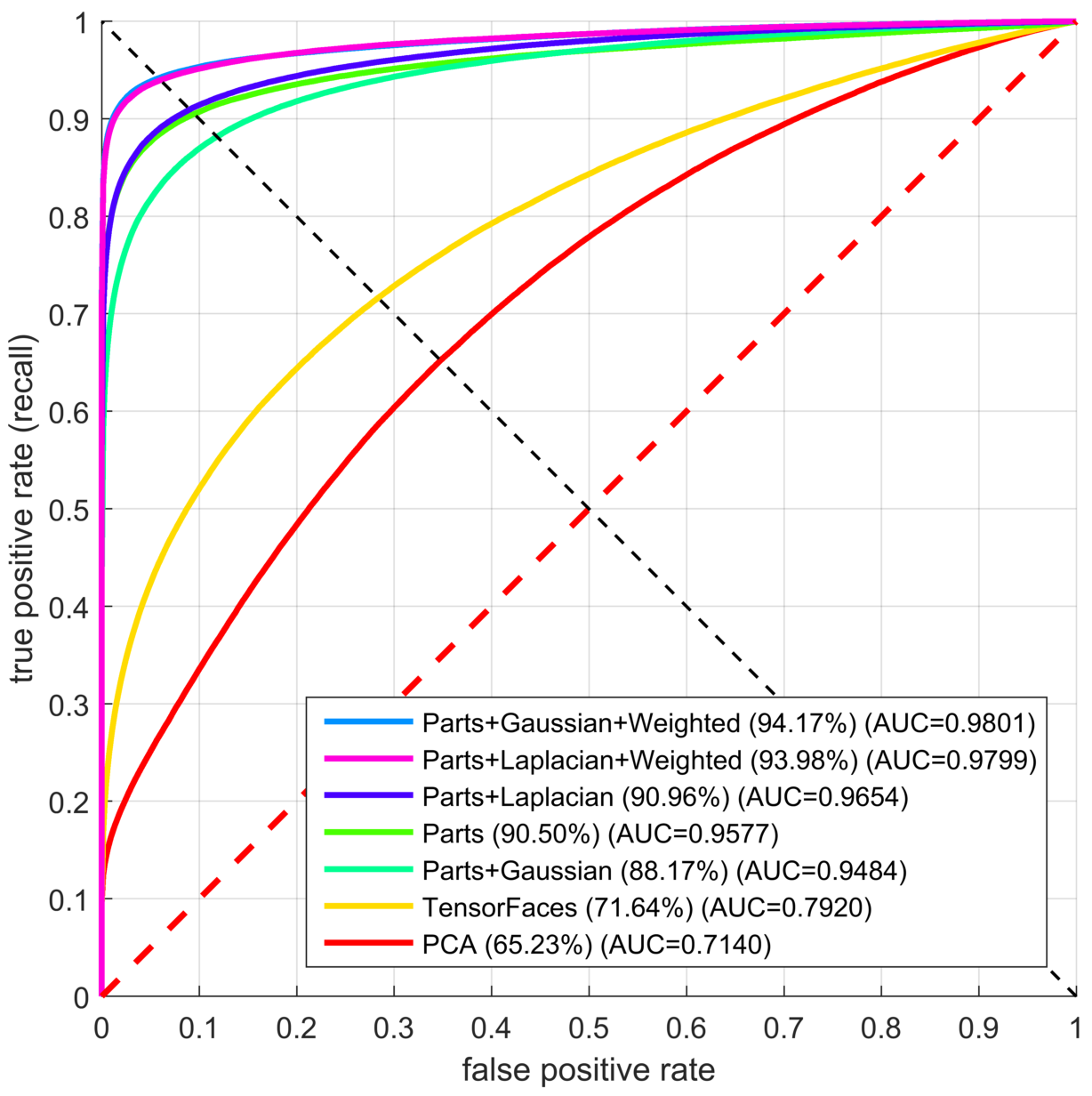
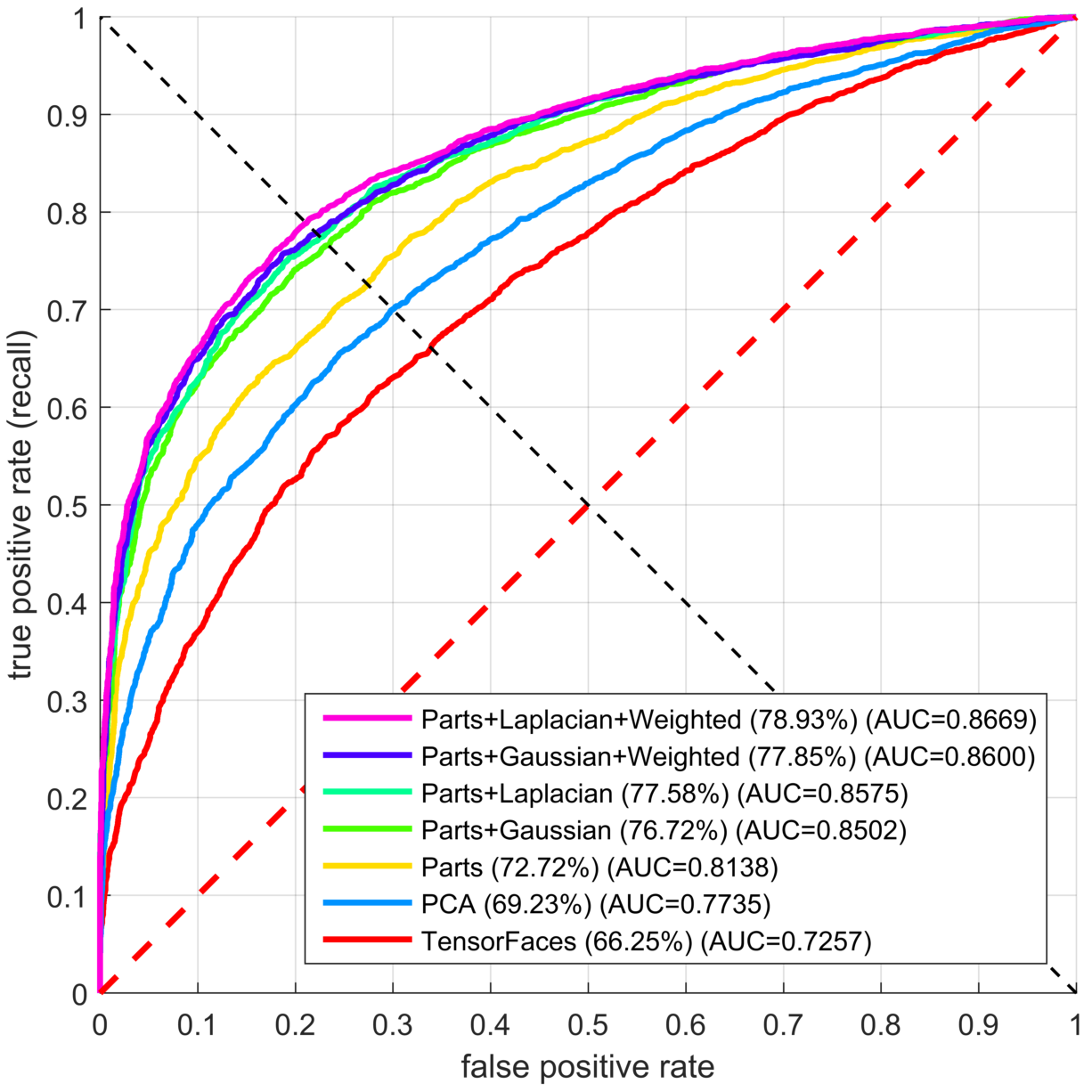
                (b)                   (c)

                                                                     (a)

Figure 4. a) Compositional Hierarchical TensorFaces learns a hierarchy of features and represents each person as a part-based compositional representation. Figure depicts the training data factorization, ${\mathbf{\mathcal{D}}}={\mathbf{\mathcal{T}}}{{}_{\mbox{\tiny${\mathbf{\mathcal{H}}}$}}}\times_{\mbox{\tiny{L}}}{\textbf{U}}_{\mbox{\tiny{L}}}\times_{\mbox{\tiny{V}}}{\textbf{U}}_{\mbox{\tiny{V}}}\times_{\mbox{\tiny{P}}}{\textbf{U}}_{\mbox{\tiny{P}}}$, where an observation is represented as ${\mathbf{d}}({\mathbf{p}},{\mathbf{v}},{{\mathbf{l}}})={\mathbf{\mathcal{T}}}{{}_{\mbox{\tiny${\mathbf{\mathcal{H}}}$}}}\times_{\mbox{\tiny{L}}}{\mathbf{l}}^{\mathrm{T}}\times_{\mbox{\tiny{V}}}{\mathbf{v}}^{\mathrm{T}}\times_{\mbox{\tiny{P}}}{\mathbf{p}}^{\mathrm{T}}$. b) ROC curves for the University of Freiburg 3D Morphable Faces dataset. c) ROC curves for the LFW dataset. The average accuracies are listed next to each method, along with the area under the curve (AUC). Parts refers to using Compositional Hierarchical TensorFaces models to separately analyze facial parts. Gaussian, Laplacian refers to using Compositional Hierarchical TensorFaces on a Gaussian/Laplacian data pyramid.

Test Dataset	PCA	TensorFaces	Compositional Hierarchical TensorFaces
			Pixels	Gaussian Pyramid	Weighted Gaussian Pyramid	Laplacian Pyramid	Weighted Laplacian Pyramid
Freiburg	65.23%	71.64%	90.50%	88.17%	94.17%	90.96%	93.98%
LFW	69.23% $\scriptstyle\pm$1.51	66.25% $\scriptstyle\pm$1.60	72.72% $\scriptstyle\pm$2.14	76.72% $\scriptstyle\pm$1.65	77.85% $\scriptstyle\pm$1.83	77.58% $\scriptstyle\pm$1.45	78.93% $\scriptstyle\pm$1.77

Table 1. Empirical results reported for LFW : PCA, TensorFaces and Compositional Hierarchical TensorFaces. Pixels denotes indepent facial part analysisGaussian/Laplacian use a multiresolution pyramid to analyze facial features at different scales. Weighted denotes a weighted nearest neighbhor.
Freiburg Experiment:
Train on Freiburg: 6 views ($\scriptstyle\pm$60^∘,$\scriptstyle\pm$30^∘,$\scriptstyle\pm$5^∘); 6 illuminations ($\scriptstyle\pm$60^∘,$\scriptstyle\pm$30^∘,$\scriptstyle\pm$5^∘), 45 people
Test on Freiburg:    9 views ($\scriptstyle\pm$50^∘, $\scriptstyle\pm$40^∘, $\scriptstyle\pm$20^∘, $\scriptstyle\pm$10^∘, 0^∘), 9 illums ($\scriptstyle\pm$50^∘, $\scriptstyle\pm$40^∘, $\scriptstyle\pm$20^∘, $\scriptstyle\pm$10^∘, 0^∘), 45 different people
LFW Experiment: Models were trained on approximately half of one percent ($0.5\%<1\%$) of the $4.4$M images used to train DeepFace.
Train on Freiburg:
15 views ($\scriptstyle\pm$60^∘,$\scriptstyle\pm$50^∘, $\scriptstyle\pm$40^∘,$\scriptstyle\pm$30^∘, $\scriptstyle\pm$20^∘, $\scriptstyle\pm$10^∘,$\scriptstyle\pm$5^∘, 0^∘), 15 illuminations ($\scriptstyle\pm$60^∘,$\scriptstyle\pm$50^∘, $\scriptstyle\pm$40^∘,$\scriptstyle\pm$30^∘, $\scriptstyle\pm$20^∘, $\scriptstyle\pm$10^∘,$\scriptstyle\pm$5^∘, 0^∘), 100 people
Test on LFW: We report the mean accuracy and standard deviation across standard literature partitions (Huang2007, ), following the
Unrestricted, labeled outside data supervised protocol.

5. Compositional Hierarchical TensorFaces

Training Data: In our experiments, we employed gray-level facial training images rendered from 3D scans of 100 subjects. The scans were recorded using a CyberwareTM 3030PS laser scanner and are part of the 3D morphable faces database created at the University of Freiburg (Blanz99, ). Each subject was combinatorially imaged in Maya from 15 different viewpoints ($\theta=-60^{\circ}$ to $+60^{\circ}$ in $10^{\circ}$ steps on the horizontal plane, $\phi=0^{\circ}$) with $15$ different illuminations ( $\theta=-35^{\circ}$ to $+35^{\circ}$ in $5^{\circ}$ increments on a plane inclined at $\phi=45^{\circ}$).

Data Preprocessing: Facial images were warped to an average face template by a piecewise affine transformation given a set of facial landmarks obtained by employing Dlib software (dlib09, ; Kazemi2014, ; Si13, ). Illumination was normalized with an adaptive contrast histogram equalization algorithm, but rather than performing contrast correction on the entire image, subtiles of the image were contrast normalized, and tiling artifacts were eliminated through interpolation. Histogram clipping was employed to avoid over-saturated regions. Each image, ${\mathbf{d}}\in\mathbb{R}^{I_{\mbox{\tiny{0}}}\times 1}$, was convolved with a set of filters $\{{\textbf{H}}_{\mbox{\tiny{s}}}\|s=1...S\}$, and the filtered images, ${\mathbf{d}}\times_{\mbox{\tiny{0}}}{\textbf{H}}_{\mbox{\tiny{s}}}$, resulted either in a Gaussian or Laplacian image pyramid. Facial parts were segmented from the various layers.

Experiments: The composite person signature was computed for every test image by employing the multilinear projection  algoritm(Vasilescu2011, ; Vasilescu07a, ), and signatures were compared with weighted nearest neighbhor.

To validate the effectiveness of our system on real-world images, we report results on “LFW” dataset (LFW)  (Huang2007, ). This dataset contains 13,233 facial images of 5,749 people. The photos are unconstrained (i.e., “in the wild”), and include variation due to pose, illumination, expression, and occlusion. The dataset consists of 10 train/test splits of the data. We report the mean accuracy and standard deviation across all splits in Table 1. Figure 4(b-c) depicts the experimental ROC curves. We follow the supervised “Unrestricted, labeled outside data” paradigm.

Results: While we cannot celebrate closing the gap on human performance, our results are promising. DeepFace, a CNN model, improved the prior art verification rates on LFW from $70\%$ to $97.35\%$, by training on $4.4M$ images of $200\times 200$ pixels from $4,030$ people, the same order of magnitude as the number of people in the LFW database. We trained on less than one percent ($1\%$) of the $4.4$M total images used to train DeepFace. Images were rendered from 3D scans of 100 subjects with an the intraocular distance of approximately 20 pixels and with a facial region captured by $10,414$ pixels (image size $\approx 100\times 100$ pixels). We have currently achieved verification rates just shy of $80\%$ on LFW. When data is limited, CNN models do not convergence or generalize.

6. Conclusion

In analogy to autoencoders which are inefficient neural network implementation of principal component analysis, a pattern analysis method based in linear algebra, CNNs are neural network implementations of tensor factorizations. This paper contributes to the tensor algebraic paradigm and models cause-and-effect as multilinear tensor interaction between intrinsic and extrinsic hierarchical causal factors of data formation. The data tensor is re-conceptualized into a hierarchical data tensor; a unified tensor model of wholes and parts is proposed; and a new compositional hierarchical tensor factorization is derived. Resulting causal factor representations are interpretable, hierarchical, and statistically invariant to all other causal factors. Our approach is demonstrated in the context of facial images by training on a very small set of synthetic images. While we have not closed the gap on human performance, we report encouraging face verification results on two test data sets–the Freiburg, and the Labeled Faces in the Wild datasets. CNN verification rates improved the $70\%$ prior art to $97.35\%$ when they employed $4.4$M images from $4,030$ people, the same order of magnitude as the number of people in the LFW database. We have currently achieved verification rates just shy of $80\%$ on LFW by employing synthetic images from 100 people for a total of less than one percent ($1\%$) of the total images employed by DeepFace. By comparison, when data is limited, CNN models do not convergence, or generalize.

References

- (1) M. Abadi, A. Agarwal, P. Barham, E. Brevdo, Z. Chen, C. Citro, G. S. Corrado, A. Davis, J. Dean, M. Devin, S. Ghemawat, I. Goodfellow, A. Harp, G. Irving, M. Isard, Y. Jia, R. Jozefowicz, L. Kaiser, M. Kudlur, J. Levenberg, D. Mané, R. Monga, S. Moore, D. Murray, C. Olah, M. Schuster, J. Shlens, B. Steiner, I. Sutskever, K. Talwar, P. Tucker, V. Vanhoucke, V. Vasudevan, F. Viégas, O. Vinyals, P. Warden, M. Wattenberg, M. Wicke, Y. Yu, and X. Zheng. TensorFlow: Large-scale machine learning on heterogeneous systems, 2015. Software available from tensorflow.org.
- (2) M. Bartlett, J. Movellan, and T. Sejnowski. Face recognition by independent component analysis. IEEE Transactions on Neural Networks, 13(6):1450–64, 2002.
- (3) F. Bastien, P. Lamblin, R. Pascanu, J. Bergstra, I. J. Goodfellow, A. Bergeron, N. Bouchard, and Y. Bengio. Theano: New features and speed improvements. Deep Learning and Unsupervised Feature Learning NIPS Workshop, 2012.
- (4) P. N. Belhumeur, J. a. P. Hespanha, and D. J. Kriegman. Eigenfaces vs. fisherfaces: Recognition using class specific linear projection. IEEE Trans. Pattern Anal. Mach. Intell., 19(7):711–720, Jul 1997.
- (5) J. Bergstra, O. Breuleux, F. Bastien, P. Lamblin, R. Pascanu, G. Desjardins, J. Turian, D. Warde-Farley, and Y. Bengio. Theano: A CPU and GPU math expression compiler. In Proc. Python for Scientific Computing Conf. (SciPy), Jun 2010. Oral Presentation.
- (6) V. Blanz and T. A. Vetter. Morphable model for the synthesis of 3D faces. In Proc. ACM SIGGRAPH 99 Conf., pages 187–194, 1999.
- (7) R. Bro. Parafac: Tutorial and applications. In Chemom. Intell. Lab Syst., Special Issue 2nd Internet Cont. in Chemometrics (INCINC’96), volume 38, pages 149–171, 1997.
- (8) C. Cadieu and B. Olshausen. Learning transformational invariants from natural movies. In Proc. 19th International Conf. on Neural Information Processing Systems, NIPS’09, page 209–216, 2009.
- (9) J. D. Carroll and J. J. Chang. Analysis of individual differences in multidimensional scaling via an N-way generalization of ‘Eckart-Young’ decomposition. Psychometrika, 35:283–319, 1970.
- (10) J. C. Chen, R. Ranjan, A. Kumar, C. H. Chen, V. M. Patel, and R. Chellappa. An end-to-end system for unconstrained face verification with deep convolutional neural networks. In IEEE International Conf. on Computer Vision Workshop (ICCVW), pages 360–368, Dec 2015.
- (11) N. Cohen, O. Sharir, and A. Shashua. On the expressive power of deep learning: A tensor analysis. In 29th Annual Conf. on Learning Theory, pages 698–728, 2016.
- (12) N. Cohen and A. Shashua. Convolutional rectifier networks as generalized tensor decompositions. In Proc. 33 rd International Conf. on Machine Learning, 2016.
- (13) R. Collobert, K. Kavukcuoglu, and C. Farabet. Torch7: A MATLAB-like environment for machine learning. In BigLearn, NIPS Workshop, number EPFL-CONF-192376, 2011.
- (14) P. Common. Independent component analysis, a new concept? Signal Processing, 36:287–314, 1994.
- (15) L. de Lathauwer. Signal Processing Based on Multilinear Algebra. PhD thesis, Katholieke Univ. Leuven, Belgium, 1997.
- (16) L. de Lathauwer. Decompositions of a higher-order tensor in block terms—part ii: Definitions and uniqueness. SIAM Journal on Matrix Analysis and Applications, 30(3):1033–1066, 2008.
- (17) L. de Lathauwer, B. de Moor, and J. Vandewalle. A multilinear singular value decomposition. SIAM Journal of Matrix Analysis and Applications, 21(4):1253–78, 2000.
- (18) L. de Lathauwer, B. de Moor, and J. Vandewalle. On the best rank-1 and rank-() approximation of higher-order tensors. SIAM Journal of Matrix Analysis and Applications, 21(4):1324–42, 2000.
- (19) L. de Lathauwer and D. Nion. Decompositions of a higher-order tensor in block terms–part iii: Alternating least squares algorithms. SIAM Journal on Matrix Analysis and Applications, page 1067–1083, 2008.
- (20) V. de Silva and L.-H. Lim. Tensor rank and the ill-posedness of the best low-rank approximation problem. SIAM Journal on Matrix Analysis and Applications, 30(3):1084–1127, 2008.
- (21) C. Figdor. Intrinsically/extrinsically. Journal of Philosophy, 105:691–718, 2008.
- (22) H. Gao, H. K. Ekenel, M. Fischer, and R. Stiefelhagen. Multi-resolution local appearance-based face verification. In Proc 20th International Conf. on Pattern Recognition (ICPR), pages 1501–04, Aug 2010.
- (23) L. Grasedyck. Hierarchical singular value decomposition of tensors. SIAM Journal on Matrix Analysis and Applications, 31(4):2019–54, 2010.
- (24) W. Hackbusch and S. Kühn. A new scheme for the tensor representation. Journal of Fourier Analysis and Applications, 15(5):706–722, 2009.
- (25) R. Harshman. Foundations of the PARAFAC procedure: Model and conditions for an explanatory factor analysis. Technical Report Working Papers in Phonetics 16, University of California, Los Angeles, Los Angeles, CA, Dec 1970.
- (26) B. Heisele, P. Ho, J. Wu, and T. A. Poggio. Face recognition: Component-based versus global approaches. Computer Vision and Image Understanding, 91:6–21, 2003.
- (27) G. E. Hinton, S. Osindero, and Y.-W. Teh. A fast learning algorithm for deep belief nets. Neural Comput., 18(7):1527–54, Jul 2006.
- (28) E. Hsu, K. Pulli, and J. Popovic. Style translation for human motion. ACM Transactions on Graphics, 24(3):1082–89, 2005.
- (29) G. B. Huang. Learning hierarchical representations for face verification with convolutional deep belief networks. In IEEE Conf. on Computer Vision and Pattern Recognition (CVPR), pages 2518–25, Jun 2012.
- (30) G. B. Huang, M. Ramesh, T. Berg, and E. Learned-Miller. Labeled faces in the wild: A database for studying face recognition in unconstrained environments. Technical Report 07-49, University of Massachusetts, Amherst, Oct 2007.
- (31) I. Humberstone. Intrinsi/extrinsic. Synthese, 108:206–267, 1986.
- (32) D. Hume. An Enquiry Concerning Human Understanding, 2nd ed. Andrew Millar, 1748.
- (33) K. Jarrett, K. Kavukcuoglu, M. Ranzato, and Y. LeCun. What is the best multi-stage architecture for object recognition? In Proc. International Conf. on Computer Vision (ICCV 2009), page 2146—53. IEEE, 2009.
- (34) V. Kazemi and J. Sullivan. One millisecond face alignment with an ensemble of regression trees. In Proc. IEEE Conf. on Computer Vision and Pattern Recognition, CVPR ’14, pages 1867–74, Washington, DC, USA, 2014. IEEE Computer Society.
- (35) Y. Kim, E. Park, S. Yoo, T. Choi, L. Yang, and D. Shin. Compression of deep convolutional neural networks for fast and low power mobile applications. CoRR, abs/1511.06530, 2015.
- (36) D. E. King. Dlib-ml: A machine learning toolkit. Journal of Machine Learning Research, 10:1755–1758, 2009.
- (37) T. G. Kolda and B. W. Bader. Tensor decompositions and applications. SIAM review, 51(3):455–500, 2009.
- (38) J. Kossaifi, A. Khanna, Z. C. Lipton, T. Furlanello, and A. Anandkumar. Tensor contraction layers for parsimonious deep nets. In Computer Vision and Pattern Recognition (CVPR), Tensor Methods in Computer Vision Workshop, pages 1940–46, Jul 2017.
- (39) H. Larochelle, D. Erhan, A. Courville, J. Bergstra, and Y. Bengio. An empirical evaluation of deep architectures on problems with many factors of variation. In Proc. 24th International Conf. on Machine Learning, ICML ’07, pages 473–480, New York, NY, USA, 2007. ACM.
- (40) V. Lebedev, Y. Ganin, M. Rakhuba, I. V. Oseledets, and V. S. Lempitsky. Speeding-up convolutional neural networks using fine-tuned cp-decomposition. CoRR, abs/1412.6553, 2014.
- (41) Y. LeCun, L. Bottou, Y. Bengio, and P. Haffner. Gradient-based learning applied to document recognition. Proceedings of the IEEE, 86(11):2278–2324, Nov 1998.
- (42) D. Lewis. Extrinsic properties. Philosophical Studies, 44:197–200, 1983.
- (43) D. K. Lewis. Causation. Journal of Philosophy, pages 556–567, 1973.
- (44) H. Li and G. Hua. Hierarchical-pep model for real-world face recognition. In IEEE Conf. on Computer Vision and Pattern Recognition (CVPR), pages 4055–64, Jun 2015.
- (45) A. M. Martinez and A. C. Kak. PCA versus LDA. IEEE Transactions on Pattern Analysis and Machine Intelligence, 23(2):228–233, Feb 2001.
- (46) P. Menzies. Intrinsic vs. extrinsic conceptions of causation. In H. Sankey, editor, Causation and the Laws of Nature, pages 313–29. 1999.
- (47) K. Murphy, A. Torralba, D. Eaton, and W. Freeman. Object Detection and Localization Using Local and Global Features, pages 382–400. Springer Berlin Heidelberg, Berlin, Heidelberg, 2006.
- (48) V. Nair and G. E. Hinton. 3d object recognition with deep belief nets. In Proc. 22Nd International Conf. on Neural Information Processing Systems, NIPS’09, pages 1339–47, USA, 2009. Curran Associates Inc.
- (49) A. Novikov, D. Podoprikhin, A. Osokin, and D. P. Vetrov. Tensorizing neural networks. In C. Cortes, N. D. Lawrence, D. D. Lee, M. Sugiyama, and R. Garnett, editors, Advances in Neural Information Processing Systems 28, pages 442–450. Curran Associates, Inc., 2015.
- (50) I. V. Oseledets. Tensor-train decomposition. SIAM Journal on Scientific Computing, 33(5):2295–2317, 2011.
- (51) O. M. Parkhi, A. Vedaldi, and A. Zisserman. Deep face recognition. In M. W. J. Xianghua Xie and G. K. L. Tam, editors, Proc. British Machine Vision Conference (BMVC), pages 41.1–41.12. BMVA Press, September 2015.
- (52) J. Pearl and C. U. Press. Causality: Models, Reasoning, and Inference. Cambridge University Press, 2000.
- (53) I. Perros, R. Chen, R. Vuduc, and J. Sun. Sparse hierarchical tucker factorization and its application to healthcare. In Proc. IEEE International Conf. on Data Mining, pages 943–948, Nov 2015.
- (54) M. Ranzato, C. Poultney, S. Chopra, and Y. LeCun. Efficient learning of sparse representations with an energy-based model. In Proc. 19th International Conf. on Neural Information Processing Systems, NIPS’06, pages 1137–44, Cambridge, MA, USA, 2006. MIT Press.
- (55) C. R. Rao and S. K. Mitra. Generalized Inverse of Matrices and its Applications. Wiley, New York, 1971.
- (56) G. Shakhnarovich and B. Moghaddam. Face recognition in subspaces. In S. Z. Li and A. K. Jain, editors, Handbook of Face Recognition, pages 141–168. Springer, New York, 2004.
- (57) W. Si, K. Yamaguchi, and M. A. O. Vasilescu. Face Tracking with Multilinear (Tensor) Active Appearance Models. Jun 2013. http://pdfs.semanticscholar.org/6c64/59d7cadaa210e3310f3167dc181824fb1bff.pdf.
- (58) N. D. Sidiropoulos, L. D. Lathauwer, X. Fu, K. Huang, E. E. Papalexakis, and C. Faloutsos. Tensor decomposition for signal processing and machine learning. IEEE Transactions on Signal Processing, 65:3551–3582, 2017.
- (59) Y. Sun, X. Wang, and X. Tang. Hybrid deep learning for face verification. In Proc. IEEE International Conf. on Computer Vision (ICCV), pages 1489–96, Dec 2013.
- (60) Y. Taigman, M. Yang, M. Ranzato, and L. Wolf. Deepface: Closing the gap to human-level performance in face verification. In Proc.IEEE Conf. on Computer Vision and Pattern Recognition (CVPR), pages 1701–08, Jun 2014.
- (61) L. R. Tucker. Some mathematical notes on three-mode factor analysis. Psychometrika, 31:279–311, 1966.
- (62) M. A. Turk and A. P. Pentland. Eigenfaces for recognition. Journal of Cognitive Neuroscience, 3(1):71–86, 1991.
- (63) M. A. O. Vasilescu. An algorithm for extracting human motion signatures. In IEEE Conf. on Computer Vision and Pattern Recognition, Hawai, 2001.
- (64) M. A. O. Vasilescu. Human motion signatures for character animation. In ACM SIGGRAPH 2001 Conf. Abstracts and Applications, Los Angeles, Aug 2001.
- (65) M. A. O. Vasilescu. Human motion signatures: Analysis, synthesis, recognition. In Proc. Int. Conf. on Pattern Recognition, volume 3, pages 456–460, Quebec City, Aug 2002.
- (66) M. A. O. Vasilescu. A Multilinear (Tensor) Algebraic Framework for Computer Graphics, Computer Vision, and Machine Learning. PhD thesis, University of Toronto, Department of Computer Science, 2009.
- (67) M. A. O. Vasilescu. Multilinear projection for face recognition via canonical decomposition. In Proc. IEEE International Conf. on Automatic Face Gesture Recognition and Workshops (FG 2011), pages 476–483, Mar 2011.
- (68) M. A. O. Vasilescu and D. Terzopoulos. Multilinear analysis for facial image recognition. In Proc. Int. Conf. on Pattern Recognition, volume 2, pages 511–514, Quebec City, Aug 2002.
- (69) M. A. O. Vasilescu and D. Terzopoulos. Multilinear analysis of image ensembles: TensorFaces. In Proc. European Conf. on Computer Vision (ECCV 2002), pages 447–460, Copenhagen, Denmark, May 2002.
- (70) M. A. O. Vasilescu and D. Terzopoulos. Multilinear subspace analysis of image ensembles. In Proc. IEEE Conf. on Computer Vision and Pattern Recognition, volume II, pages 93–99, Madison, WI, 2003.
- (71) M. A. O. Vasilescu and D. Terzopoulos. TensorTextures: Multilinear image-based rendering. ACM Transactions on Graphics, 23(3):336–342, Aug 2004. Proc. ACM SIGGRAPH 2004 Conf., Los Angeles, CA.
- (72) M. A. O. Vasilescu and D. Terzopoulos. Multilinear independent components analysis. In Proc. IEEE Conf. on Computer Vision and Pattern Recognition, volume I, pages 547–553, San Diego, CA, 2005.
- (73) M. A. O. Vasilescu and D. Terzopoulos. Multilinear projection for appearance-based recognition in the tensor framework. In Proc. 11th IEEE International Conf. on Computer Vision (ICCV’07), pages 1–8, Rio de Janeiro, Brazil, 2007.
- (74) D. Vlasic, M. Brand, H. Pfister, and J. Popovic. Face transfer with multilinear models. ACM Transactions on Graphics (TOG), 24(3):426–433, Jul 2005.
- (75) Y. Wong, M. T. Harandi, C. Sanderson, and B. C. Lovell. On robust biometric identity verification via sparse encoding of faces: Holistic vs local approaches. In Proc. International Joint Conf. on Neural Networks (IJCNN), pages 1–8, June 2012.
- (76) C. Xiong, L. Liu, X. Zhao, S. Yan, and T. K. Kim. Convolutional fusion network for face verification in the wild. IEEE Transactions on Circuits and Systems for Video Technology, 26(3):517–528, Mar 2016.
- (77) Z. Xu, H. Chen, S. Zhu, and J. Luo. A composite template for human face modeling and sketch. IEEE Transations on Pattern Analysis and Machine Intelligence, 30:955–969, 2008.
- (78) M.-H. Yang. Face recognition using kernel methods. In Proc. 14th International Conf. on Neural Information Processing Systems: Natural and Synthetic, NIPS’01, pages 1457–64, Cambridge, MA, USA, 2001. MIT Press.