Multi-Agent Connected Autonomous Driving using Deep Reinforcement Learning

Abstract

The capability to learn and adapt to changes in the driving environment is crucial for developing autonomous driving systems that are scalable beyond geo-fenced operational design domains. Deep Reinforcement Learning (RL) provides a promising and scalable framework for developing adaptive learning based solutions. Deep RL methods usually model the problem as a (Partially Observable) Markov Decision Process in which an agent acts in a stationary environment to learn an optimal behavior policy. However, driving involves complex interaction between multiple, intelligent (artificial or human) agents in a highly non-stationary environment. In this paper, we propose the use of Partially Observable Markov Games(POSG) for formulating the connected autonomous driving problems with realistic assumptions. We provide a taxonomy of multi-agent learning environments based on the nature of tasks, nature of agents and the nature of the environment to help in categorizing various autonomous driving problems that can be addressed under the proposed formulation. As our main contributions, we provide MACAD-Gym, a Multi-Agent Connected, Autonomous Driving agent learning platform for furthering research in this direction. Our MACAD-Gym platform provides an extensible set of Connected Autonomous Driving (CAD) simulation environments that enable the research and development of Deep RL- based integrated sensing, perception, planning and control algorithms for CAD systems with unlimited operational design domain under realistic, multi-agent settings. We also share the MACAD-Agents that were trained successfully using the MACAD-Gym platform to learn control policies for multiple vehicle agents in a partially observable, stop-sign controlled, 3-way urban intersection environment with raw (camera) sensor observations.

1 Introduction

Driving involves complex interactions between other agents that is near-impossible to be exhaustively described through code or rules. Autonomous driving systems for that reason cannot be pre-programmed with exhaustive rules to cover all possible interaction mechanisms and scenarios on the road. Learning agents can potentially discover such complex interactions automatically through exploration and evolve their behaviors and actions to be more successful in driving based on their experiences gathered through interactions with the driving environment (over time and/or in simulation). The Deep RL framework [18] [6] provides a scalable framework for developing adaptive, learning-based solutions for such problems. But, it is hard to apply RL algorithms to live systems [5], especially robots and safety-critical systems like autonomous cars and RL-based learning is not very sample efficient [5] One way to overcome such limitations is by using realistic simulation environments to train these agents and transfer the learned policy to the actual car. High-fidelity Autonomous driving simulators like CARLA [4] and AirSim [23] provide a simulation platform for training Deep RL agents in singe-agent driving scenarios.

In single-agent learning frameworks, the interaction between other agents in the environment or even the existence of other agents in the environment is often ignored. In Multi-Agent learning frameworks, the interaction between other agents can be explicitly modeled.

Connectivity among vehicles are becoming ubiquitous and viable through decades of research in DSRC and other vehicular communication methods. With the increasing deployment of 5G infrastructure for connectivity and the increasing penetration of autonomous vehicles with connectivity and higher levels of autonomy [22], the need for the development of methods and solutions that can utilize connectivity to enable safe, efficient, scalable and economically viable Autonomous Driving beyond Geo-fenced areas has become very important to our transportation system.

Autonomous Driving problems involve autonomous vehicles navigating safely and socially from their start location to the desired goal location in complex environments which involve multiple, intelligent actors whose intentions are not known by other actors. Connected Autonomous Driving makes use of connectivity between vehicles (V2V), between vehicles and infrastructure (V2I), between vehicles and pedestrians (V2P) and between other road-users.

CAD problems can be approached using homogeneous, communicating multi-agent driving simulation environments for research and development of learning based solutions. In particular, such a learning environment enables training and testing of RL algorithms. To that end, in this paper,… 1. We propose the use of Partially Observable Markov Games for formulating the connected autonomous driving problems with realistic assumptions. 2. We provide a taxonomy of multi-agent learning environments based on the nature of tasks, nature of agents and the nature of the environment to help in categorizing various autonomous driving problems that can be addressed under the proposed formulation. 3. We provide MACAD-Gym, a multi-agent learning platform with an extensible set of Connected Autonomous Driving (CAD) simulation environments that enable the research and development of Deep RL based integrated sensing, perception, planning and control algorithms for CAD systems with unlimited operational design domain under realistic, multi-agent settings. 4. We also provide MACAD-Agents, a set of baseline/starter agents to enable the community to conduct learning experiments and train agents using the platform. The results of multi-agent policy learning by one of the provided baseline approach, trained in a partially observable, stop-sign controlled, 3-way urban intersection environment with raw, camera observations are summarized in 5. experimental results in a multi-agent settings with raw, simulated camera/sensor observations to learn heterogeneous control policies to pass through a signalized, 4-way, urban intersection in a partially observable multi-agent, CAD environment with two cars, a pedestrian and a motor cyclist where all the actors are controlled by our MACAD-Agents. Figure 1 depicts an overview of one of the MACAD environments released as a part of the MACAD-Gym platform.

The rest of the paper is organized as follows: We discuss how partially-observable markov games (POMG) can be used to model connected autononomous driving problems in 2. We then provide an intuitive classification of the tasks and problems in the CAD space in section 3 and discuss the nomenclature of the MACAD-Gym environments in section 3.4. We provide a quick overview of multi-agent deep RL algorithms in the context of CAD in section 4 and conclude with a brief discussion about the result obtained using MACAD-Agents in a complex multi-agent driving environment.

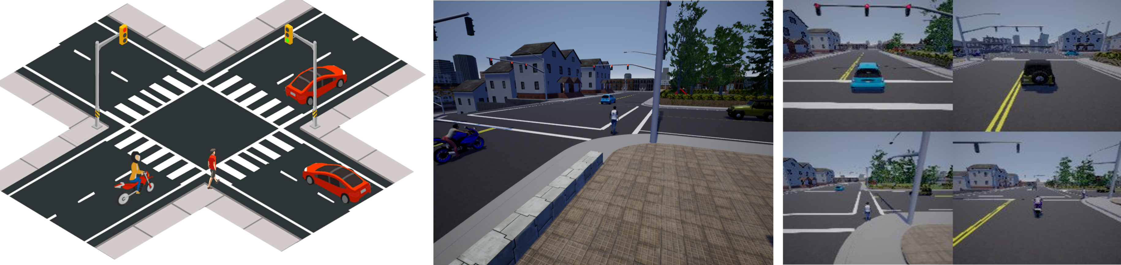
Figure 1: Figure shows a heterogeneous multi-agent learning environment created using MACAD-Gym. An overview of the scenario is shown in the left image. The middle image shows the simulated scenario and the right image shows tethered views of each agent’s observation

2 Connected Autonomous Driving as Partially Observable Markov Games

In single-agent learning settings, the interaction between the main agent and the environment is modeled as part of a Markov Decision Process (MDP). Other agents (if) present are and treated to be part of the environment irrespective of their nature (cooperative, competitive), type (same/different as the main agent) and sources of interactions with the main agent. Failing to account for the presence of other intelligent/adaptive agents in the environment leads to conditions that violate the stationary and Markov assumptions of the underlying learning framework. In particular, when other intelligent agents that are capable of learning and adapting their policies are present, the environment becomes non-stationary.

2.1 Formulation

One way to generalize the MDP to account for multiple agents in multiple state configurations is using Markov Games [16] which re defines the game- theoretic stochastic games [24] formulation in the reinforcement learning context. In several real-world multi-agent problem domains like autonomous driving, assuming that each agent can observe the complete state of the environment without uncertainty is unrealistic, partly due to the nature of the sensing capabilities present in the vehicle (actor), the physical embodiment of the agent. Partially Observable Stochastic Games (POSG) [7] extend stochastic games to problems with partial observability. In the same vein as Markov Games, we re-define POSG in the context of reinforcement learning as Partially Observable Markov Games, POMG in short, as a tuple $\langle\mathcal{I},\mathcal{S},\mathcal{A},\mathcal{O},\mathcal{T},\mathcal{R}\rangle$ in which,

$\mathbf{I}$ is a finite set of actors/agents

$\mathcal{S}$ is the finite set of states

$\mathcal{A}=\times_{i\in I}\mathcal{A}_{i}$ is the set of joint actions where $\mathcal{A}_{i}$ is the set of actions available to agent $i$.

$\mathcal{O}=\times_{i\in I}\mathcal{O}_{i}$ is the set of join observations where $\mathcal{O}_{i}$ is the set of observations for agent i.

$\mathcal{T}=\mathcal{P}(\mathbf{s^{\prime}},\mathbf{o}|\mathbf{s},\mathbf{a})$ is the Markovian state transition and observation probability that taking a joint action $\mathbf{a}=\langle a_{1},...a_{n}\rangle$ in state $s$ results in a transition to state $s^{\prime}$ with a join observation $\mathbf{o}=\langle o_{1},...o_{n}\rangle$

$\mathcal{R}_{i}:\mathcal{S}\times\mathcal{A}\to\mathbb{R}$ is the reward function function for agent $i$

At each time step $t$, the environment emits a joint observation $\mathbf{o}=\langle o_{1},\cdots,o_{n}\rangle$ from which each agent $i$ directly observes its component $o_{i}\in\mathcal{O}_{i}$ and takes action $a_{i}\in A_{i}$ based on some policy $\pi_{i}:\mathcal{O}_{i}\times\mathcal{A}_{i}\to[0,1]$ and receives a reward $r_{i}$ based on the reward function $\mathcal{R}_{i}$ .

Note that, the above formulation is equivalent to a POMDP when $n=1$ (single-agent formulation).

While a POSG formulation of the autonomous driving problem enables one to approach the problem with out making unrealistic assumptions, it does not enable computationally tractable methodologies to solve the problem except under simplified, special structures and assumptions like two-player zero-sum POSGs. In the next section, we discuss the practical usage in the CAD domain.

2.2 Practical usage in Connected Autonomous Driving

The availability of a communication (whether through explicit communication semantics or implicitly through augmented actions) channel between the agents (and/or the env) in the CAD domain, enable the sharing/transaction of local information (or private beliefs) that can provide information about some (or whole) subset of the state which is locally observable by other agents, make solutions computationally tractable even as the size of the problem (eg: num agents) increases. We realize that such a transaction of local information would give rise to issue of integrity, trust and other factors. The interaction between different agents and the nature of their interaction can be explicitly modeled using a communication channel. In the absence of an explicit communication channel, the incentives for the agents to learn to cooperate or compete, depends on their reward functions. The particular case in which all the agents acting in a partially observable environment share the same reward function, can be studied under the DEC- POMDP [19] formulation. But not all problems in CAD have the agent’s rewards completely aligned (or completely opposite).

We consider Multi-Agent Driving environments with $n$ actors, each controlled by an agent, indexed by $i$. At any given time, $t$, the state of the agent $i$ is defined to be the state of the actor under its control and it is represented as ${s}_{i}\in\mathcal{S}$ where $\mathcal{S}$ is the state space. The agent can choose an action $a_{i}\in\mathcal{A}_{i}$ , where $\mathcal{A}_{i}$ is the action space of agent $i$ which, could be different for different actors. While the environment is non-Markov from each of the agent’s point of view, the driving world as a whole is assumed to be Markov i.e, given the configuration of all the $n$ actors at time $t$ : $\mathbf{s}=[s_{1},...s_{n}]$ , their actions $\mathbf{a}=[a_{1},...a_{n}]$, and the state of the environment $E$, the evolution of the system is completely determined by the conditional transition probability $\mathcal{T}(\mathbf{s^{\prime}},\mathbf{o},E^{\prime}|\mathbf{s},E,\mathbf{a})$. This assumption allows us to apply and scale distributed RL algorithms that are developed for the single-agent MDPs to the Multi-Agent setting.

The explicit separation of the join state of the agents $\mathbf{s}_{i}$ from the state of the environment $E$ at time $t$ in the driving world, facilitates agent implementations to learn explicit models for the environment, in addition to learning models for other agents or the world model as a whole.

Under the proposed formulation for multi-agent CAD, at every time step $t$, each actor (and hence the agent) receives an observation $o_{i}$, based on its state $s_{i}$ and the (partial) state of the environment $E_{i}$ and possibly, (partial) information $I(\mathbf{s_{-i}},E_{-i})$ about the state of other agents $\mathbf{s_{-i}}=[s_{j}]_{j\neq i}$ and the state of the environment $E_{-i}$ that is not directly observable.

The observation $o_{i}$ can be seen as some degraded function $\phi(s_{i},E)$ of the full state of agent i . In reality, the nature and the degree of degradation arises from the sensing modalities and the type of sensors (camera, RADAR, LIDAR, GPS etc.) available to the vehicle actors. Connectivity through IEEE 802.11 based Dedicated Short-Range Communications (DSRC) [14] or cellular modems based C-V2X [28] enables the availability of the information $I(\mathbf{s_{-n}},E_{-i})$ about other agents and non-observable parts of the environment through Vehicle-to-Vehicle (V2V), Vehicle-to-Infrastructure (V2I) or Vehicle-to-Anything (V2X) communication.

The goal of each agent is to take actions $a_{i}$ for the vehicle actor that is under its control based on its local state $[o_{i},I(\mathbf{s_{-i},E_{-i}})]$ in order to maximize its long term cumulative reward over a time horizon T with a discount factor of $\gamma$.

3 Multi-Agent Connected Autonomous Driving Platform

The connected-autonomous driving domain poses several problems which can be categorized into sensing, perception, planning or control. Learning algorithms can be used to solve the tasks in an integrated/end-to-end fashion [13] [3] or in an isolated approach for each driving task like intersection-driving [12] [21] and lane-changing [27].

Driving tasks falling under each of the above categories can be further divided and approached, depending on the combination of the nature of the tasks, the nature of the environments and the nature of the agents. The following subsections provide a brief discussion on such a classification of multi-agent environments that are supported on the MACAD-Gym platform, to enable the development of solutions for various tasks in the the CAD domain.

3.1 Nature of tasks

The nature of the task in a driving environment is determined based on the desired direction of focus of the task specified through the design of experiments.

Independent

Multi-agent driving environments in which each actor is self-interested/selfish and has its own, often unique objective, fall under this category. One way to model such setup is by treating the environment to be similar to a single-agent environment with all the actors apart from the host actor are treated to be be part of the environment. Such environments help in developing non-communicating agents that doesn’t rely on explicit communication channels. Such agents will benefit from agents modeling agents [1].

Cooperative

Cooperative CAD environments help in developing agent algorithms that can learn near-globally optimal policies for all the driving agents that act as a cooperative unit. Such environments help in developing agents that learn to communicate [9] and benefit from learning to cooperate [25]. This type of environments will enable development of efficient fleet of vehicles that cooperate and communicate with each other to reduce congestion, eliminate collisions and optimized traffic flows.

Competitive

Competitive driving environments allow the development of agents that can handle extreme driving scenarios like road-rages. The special case of adversarial driving can be formulated as a zero-sum stochastic game, which can be cast as a MDP and solved which has useful properties and properties and results including: value Iteration, unique solution to Q*, independent computation of policies and representation of policies using Q functions as discussed in [26]. Agents developed in competitive environments can be used for law enforcement and or other use cases including the development of strong adversarial driving actors to help improve handling capabilities of driving agents.

Mixed

Some tasks that are designed to be of a particular nature may still end up facilitating approaches that stretch the interaction to other types of tasks. For example, an agent operating in an environment on a task which is naturally (by design) an independent task can learn to use mixed strategies of being cooperative at times and being competitive at times in order to maximize it’s own rewards. Emergence of such mixed strategies [17] is another interesting research area supported in MACAD-Gym, that can lead to new traffic flow behaviors.

3.2 Nature of agents/actors

Homogeneous

When all the road actors in the environment belong to one class of actors (eg. only cars or only motor-cyclists), the action space of each actor can be the same and the interactions are limited to be between a set of homogeneous driving agents.

Heterogeneous

Depending on the level of detail in the environment representation (a traffic light could be represented as an intelligent actor), majority of autonomous driving tasks involve interaction between a heterogeneous set of road actors.

Communicating

Actors that are capable of communicating (through direct or indirect channels [20] with other actors through Vehicle-to-Vehicle (V2V) communication channels can help to increase information availability in partially-observable environments. Such communication capabilities allow for training agents with data augmentation wherein the communication acts as a virtual/shared/crowd-sourced sensor. Note that, Pedestrian (human) agents can be modeled as communicating agents that use (hand and body) gestures transmit information and can receive information using visual (external display/signals on cars, Traffic signals etc) and auditory (horns, etc).

Non-communicating

While the environment provides or allows for a communication channel, if an agent is not capable of communicating/making-use-of-the-communication channel by virtue of the nature of the actor, it is grouped under this category. Example include vehicle actors that have no V2X communication capability.

3.3 Nature of environments

Full/partial observability

In order for an environment to be fully observable, every agent in the environment should be able to observe the complete state of the environment at every point in time. Driving environments under realistic assumptions are partially-observable environments. The presence of connectivity (V2V, V2X/cloud) in CAD environments make the problems in PO environments more tractable.

Synchronous/Asynchronous

In a synchronous environment, all the actors are required to take an action in a time synchronous manner. Whereas, in asynchronous environments, different actors can act at different frequencies.

Adversarial

If there exists any environmental factor/condition that can stochastically impair the ability of the agents in the environment to perform at their full potential, such cases are grouped under adversarial environments. For example, the V2X communication medium can be perturbed/altered by the environment,which enables the study of the robustness of agents under adversarial attacks. Bad weather including snowy, rainy or icy conditions also can be modeled and studied under adversarial environments. Injection of "impulse"/noise that are adversarial in nature help in validating the reliability of agent algorithms.

Table 1 in appendix B shows a short list of environments that are supported by the MACAD-Gym platform.

3.4 MACAD-Gym Environment Naming Conventions

A naming convention that conveys the environment type, nature of the agent, nature of the task, nature of the environment with version information is proposed. The naming convention follows the widely used convention in the community introduced in [2] but, has been extended to be more comprehensive and to accommodate more complex environment types suitable for the autonomous driving domain.

The naming convention is illustrated below with HeteCommCoopPOUrbanMgoalMAUSID as the example:

$$\underset{\underset{\text{Nature of Agents}}{\downarrow}}{\underbrace{\overset{\overset{\begin{subarray}{c}\{\text{Hete},\\ \text{Homo}\}\end{subarray}}{\uparrow}}{\overbrace{\text{Hete}}}\overset{\overset{\begin{subarray}{c}\{\text{Comm},\\ \text{Ncom\}}\end{subarray}}{\uparrow}}{\overbrace{\text{Comm}}}}}\underset{\underset{{\text{Nature of tasks}}}{\downarrow}}{\underbrace{\overset{\overset{\begin{subarray}{c}\{Inde,\\ Coop,\\ Comp,\\ Mixd\}\end{subarray}}{\uparrow}}{\overbrace{\text{Coop}}}}}\underset{\underset{{\text{Nature of environment}}}{\downarrow}}{\underbrace{\overset{\overset{\begin{subarray}{c}\{PO,\\ FO\}\end{subarray}}{\uparrow}}{\overbrace{\text{PO}}}\overset{\overset{\begin{subarray}{c}\{Bridg,\\ Freew,\\ Hiway,\\ Intrx,\\ Intst,\\ Rural,\\ Tunnl,\\ Urban\}\end{subarray}}{\uparrow}}{\overbrace{\text{Urban}}}\overset{\overset{\begin{subarray}{c}\{\hbox{},\\ Advrs,\\ Async,\\ Mgoal,\\ Synch,\\ ...\}\end{subarray}}{\uparrow}}{\overbrace{\text{Mgoal}}}\overset{\overset{\begin{subarray}{c}\{MA,\\ SA\}\end{subarray}}{\uparrow}}{\overbrace{\text{MA}}}}}\overset{\overset{\begin{subarray}{c}Unique\\ Scenario\\ ID\end{subarray}}{\uparrow}}{\overbrace{\text{USID}}}\text{-}\underset{\underset{\text{version}}{\downarrow}}{\underbrace{\text{v0}}}$$

A few example environments that are part of the initial Carla-Gym platform release are listed in Appendix B.

The above description summarizes the naming convention to accommodate various types of driving environments with an understanding that several scenarios and their variations can be created by varying the traffic conditions, speed limits and behaviors of other (human-driven, non-learning, etc) actors/objects in each of the environments. The way these variations are accommodated in the platform is by using an Unique Scenario ID (USID) for each variation in the scenario. The "version" string allows versioning each scenario variation when changes are made to the reward function and/or observation and actions spaces.

4 Multi-Agent Deep Reinforcement Learning For Connected Autonomous Driving

In the formulation presented in section 2, formally, the goal of each agent is to maximize the expected value of its long-term future reward given by the following objective function:

$$J_{i}(\pi_{i},\boldsymbol{\pi_{-i}})=\mathbb{E}_{\pi_{i},\boldsymbol{\pi_{-i}}}[R_{i}]=\mathbb{E}_{\pi_{i},\boldsymbol{\pi_{-1}}}[\sum^{T}_{t=0}\gamma^{t}r_{i}(\boldsymbol{s},a_{i})]$$ (1)

Where $\boldsymbol{\pi}_{-i}=\prod_{j}{\pi_{j}(\mathbf{s},a_{j}),{j\neq i}}$ is the set of policies of agents other than agent $i$. In contrast to the single-agent setting, the objective function of an agent in the multi-agent setting depends on the policies of the other agents.

4.1 Value Based Multi-Agent Deep Reinforcement Learning

$$V_{i}^{\boldsymbol{\pi}}(s)=\sum_{\mathbf{a}\in\mathbf{A}}\boldsymbol{\pi}(s,\mathbf{a})\sum_{s^{\prime}\in\mathbf{S}}T(s,a_{i},\mathbf{a_{-i}},s^{\prime})[R(s,a_{i},\mathbf{a_{-i}},s^{\prime})+\gamma V_{i}^{\boldsymbol{\pi}}(s^{\prime})]$$ (2)

where, $s=(\mathbf{S}^{t},E^{t})$, $\mathbf{a}=(a_{i},\mathbf{a_{-i}})$, $\boldsymbol{\pi}(s,\mathbf{a})=\prod_{j}{\pi_{j}(s,a_{j})}$

The optimal policy is a best response dependent on the other agent’s policies,

$$\pi_{i}^{*}(s,a_{i},\boldsymbol{\pi}_{-i})={\operatorname*{argmax}_{\pi_{i}}}V_{i}^{(\pi_{i},\boldsymbol{\pi}_{-i})}(s)$$ (3)

$$=\operatorname*{argmax}_{\pi_{i}}\sum_{\mathbf{a}\in A}\pi_{i}(\mathbf{s},a_{i})\boldsymbol{\pi}_{-i}(\mathbf{s},\mathbf{a}_{-i})\sum_{s^{\prime}\in\mathcal{S}}\mathcal{T}(\mathbf{s},a_{i},\mathbf{a}_{-i},s^{\prime})[R(\mathbf{s},a_{i},\mathbf{a}_{-i},s^{\prime})+\gamma V_{i}^{(\pi_{i},\boldsymbol{\pi}_{-i})}(s^{\prime})]$$ (4)

Computing the optimal policy under this method requires $\mathcal{T}$, the transition model of the environment to be known. The state-action value function $Q_{i}^{*}(s_{i},a_{i}|\boldsymbol{\pi}_{-i})$ is presented in appendix B.

4.2 Policy Gradients

If $\boldsymbol{\theta}=\{\theta_{1},\theta_{2},...,\theta_{N}\}$ represents the parameters of the policy $\boldsymbol{\pi}=\{\pi_{i},\pi_{2},...,\pi_{N}\}$, The gradient of the objective function (equation 1) w.r.t the policy parameters can be written as:

$$\nabla_{\theta_{i}}J_{i}(\pi_{i},\boldsymbol{\pi}_{-i})=\mathbb{E}_{\boldsymbol{S}^{t},E^{t}\sim{p^{\boldsymbol{\pi}}}}$$ (5)

4.3 Decoupled Actor - Learner architectures

For a given CAD situation with N homogeneous driving agents, the globally optimal solution is the policy that maximizes the following objective:

$$\mathbb{E}_{\pi}[\sum_{i=1}^{N}R_{i}]=\sum_{i=1}^{N}\mathbb{E}_{\pi_{i},\boldsymbol{\pi_{-i}}}[R_{i}]$$ (6)

The straight-forward approach to optimize for the global objective (equation 6) amounts to finding the globally optimal policy:

$$\boldsymbol{\pi}^{g^{*}}=\operatorname*{argmax}_{\pi}\sum_{i=1}^{N}J_{i}(\pi_{i},\boldsymbol{\pi_{-i}})$$ (7)

However, this approach requires access to policies of all the agents in the environment.

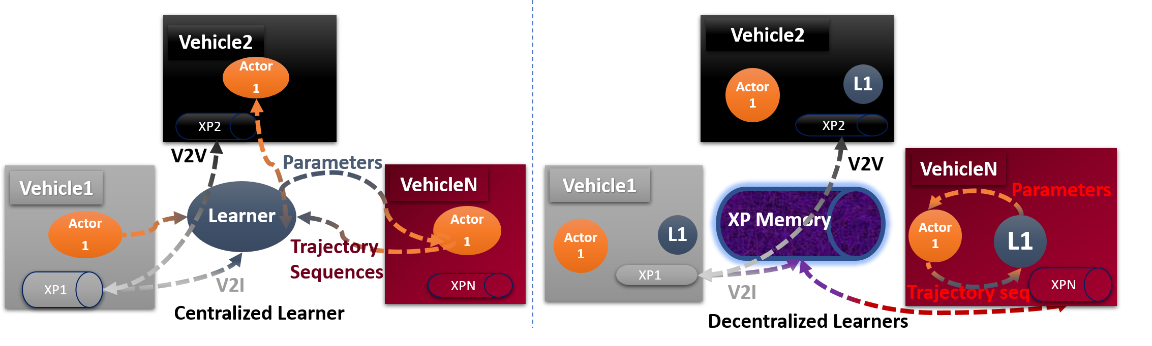
Figure 2: Centralized learner (left) and decentralized learner(right) architecture for connected-autonomous driving

Centralized Learners

Figure 2 (left) depicts decoupled actor-learner architecture with a centralized learner which can be used to learn a globally-optimal driving policy $\boldsymbol{\pi}^{g^{*}}$.

Decentralized Learners

In the most general case of CAD, each driving agent follows it’s own policy that is independent of the other agent’s driving policy. Note that this case can be extended to cover those situations where some proportion of the vehicles are driven by humans who have their own intentions and policies.

Each agent can independently learn, to find policies that optimize their local objective function (equation 1). One such architecture for CAD is shown in figure 2 (right).

Shared Parameters

With connectivity as in CAD, some are all the parameters of each agent’s policy can be shared with one another. Such parameter sharing between driving agents can be implemented with both centralized and decentralized learner architectures.

Shared Observations

Sharing observations from the environment with other agents via communication medium, reduces the gap between the observation $o_{i}$ and the true state $\langle s_{i},E\rangle$ and can drive the degradation function $\phi(s_{i},E)$ (discussed in section 2.2) to Identity (no degradation).

Shared Experiences

This enables collective experience replay which can theoretically lead to gains in a way similar to distributed experience replay [11] in single-agent setting.

Shared policy

If all the vehicles follow the same policy $\pi^{l}$, it follows from equation 1 that the learning objective for each of the agents can be simplified, resulting in an identical and equal definition:

$$J(\pi^{l})=\mathbb{E}_{\pi^{l}}[\sum_{t=0}^{T}\gamma^{t}r_{i}(\mathbf{S}^{t},E^{t},a_{i}^{t})]$$ (8)

In this setting, challenges due to the non-stationarity of the environment is subsided due to the perfect knowledge about other agent’s policies. In practice this case is of use in autonomous fleet operations in controlled environments where all the autonomous driving agents can be designed to follow the same policy

5 Experiments and Conclusion

We trained MACAD-Agents in the HomoNcomIndePOIntrxMASS3CTWN3-v0 environment, which is a stop sign-controlled urban intersection environment with homogeneous, non-communicating actors, each controlled using the IMPALA [8] agent architecture. The actors car1(red cola van), car2(blue minivan), car3 (maroon sedan) learn a reasonably good driving policy to completely cross the intersection without colliding and within the time-limit imposed by the environment. The environment is depicted in Figure 3 along with the cumulative mean and max rewards obtained by the 3-agent system. Complete details about the experiment including agent-wise episodic rewards are presented in appendix C.

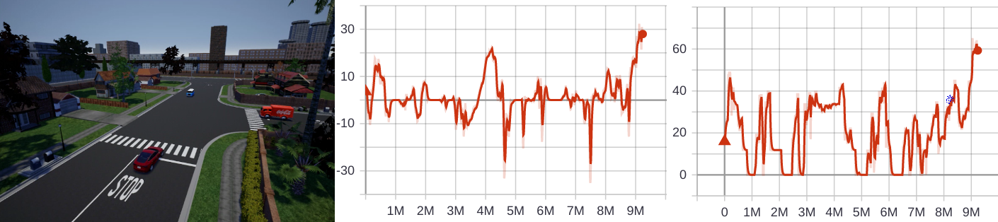
Figure 3: Figure shows a start state in the ‘HomoNcomIndePOIntrxMASS3CTWN3-v0‘ environment (left) and the cumulative mean episode rewards (middle) and the cumulative max episode rewards (right) obtained by the 3-agent system.

To conclude, we described a POSG formulation and discussed how CAD problems can be studied under such a formulation for various categories of tasks. We presented the opensource MACAD-Gym platform and the starter MACAD-Agents to help researchers to explore the CAD domain using deep RL algorithms We also provided preliminary experiment results that validated the MACAD-Gym platform by conducting a starter experiment with the MACAD-Agents in a multi-agent driving environment and discussed the results showing the ability of the agents to learn independent vehicle control policies from high-dimensional raw sensory (camera) data in a partially-observed, multi-agent simulated driving environment. The MACAD-Gym platform enables training driving agents for several challenging autonomous driving problems. As a future work, we will develop a benchmark with a standard set of environments that can serve as a test-bed for evaluating machine-learning-based CAD driving agent algorithms.

Appendix A AppendixA

A.1 Actor - Agent disambiguation

In the context of this paper, to avoid any ambiguity between the usage of the terms, we consider an actor to be a physical entity with some form of embodied intelligence, acting in an environment. We consider an agent to be a (software/algorithm) entity that provides the intelligence to an actor. The agent can learn and/or adapt based on its interaction with the environment by controlling the (re)action of the actor.

A.2 Available and supported environments in the MACAD-Gym platform

A short-list of CAD environments made available on the MACAD-Gym platform are listed below with a brief description:

Table 1: An example list of environments that are part of the carla-gym platform with a description to explain the naming conventions to make it easy for the community to add new classes of environments.

Environment Name	Description
HomoNcomIndePOIntrxMASS3CTwn3-v0	Homogeneous Noncommunicating, Independent, Partially-Observable Intersection, Multi-Agent Environment with a Stop Sign, 3Car scenario in Town03 version-0
HeteCommIndePOIntrxMAEnv-v0	Heterogeneous Communicating, Independent, PartiallyObservableIntersection Multi-Agent Environment version 0
HeteCommCoopPOUrbanMAEnv-v0	Heterogeneous Communicating, Cooperative, , Partially-Observable, Urban Multi-Agent Environment version 0
HomoNcomIndeFOHiwaySynchMAEnv-v0	Homogeneous Noncommunicating, Independent, Fully-Observable, Highway, Multi-Agent Environment version-0

Table 2: Supported MA environment types

		Independent	Cooperative	Competitive
Homogeneous	Communicating	✓	✓	✓
	Non-Communicating	✓	✓	✓
Heterogeneous	Communicating	✓	✓	✓
	Non-Communicating	✓	✓	✓

Appendix B Appendix B

B.1 State-action value function

In a fully-observable, Single-Agent setting, the optimal action-value function $Q^{*}(s,a)$ can be estimated using the following equation:

$$Q^{*}(s,a)=\mathbb{E}_{s^{\prime}}[r+\gamma max_{a^{\prime}}Q^{*}(s^{\prime},a^{\prime})|s,a].$$ (9)

DQN [18] uses a neural network to represent the action-value function parametrized by $\theta$, $Q(s,a;\theta)$. The parameters are optimized iteratively by minimizing the Mean Squared Error (MSE) between the Q-network and the Q-learning target using Stochastic Gradient Descent with the loss function given by:

$$\mathcal{L}(\theta)=\mathbb{E}_{s,a,r,s^{\prime}\sim\mathcal{D}}[(r+\gamma max_{a}^{\prime}Q(s^{\prime},a^{\prime};\theta^{-})-Q(s,a;\theta))^{2}]$$ (10)

where $\mathcal{D}$ is the experience replay memory containing $(s_{t},a_{t},r_{t},s^{\prime})$ tuples.

For a fully-observable, Multi-Agent setting, the optimal action-value function $Q^{*}(s,a|\pi_{-i})$ can be estimated using the following equation:

$$\begin{split}Q^{*}(s,a|\pi_{-i})=\sum_{a_{-i}}\pi_{-i}(a_{-i},s)\mathbb{E}_{s^{\prime}}[r_{i}(s,a,s^{\prime})\\ +\gamma\mathbb{E}_{a^{\prime}}[Q^{*}(s^{\prime},a^{\prime}|\pi_{-i})]]\end{split}$$ (11)

where $\pi_{-i}$ is the joint policy of all agents other than agent $i$, $s$ and $a$ are the state and action of agent $i$ at time-step $t$ and $s^{\prime}$, $a^{\prime}$ are the state and action of agent $i$ at time-step $t+1$.

Independent DQN [25] extends DQN to cooperative, fully-observable Multi-Agent setting, applied to a two-player pong environment, in which all agents independently learn and update their own Q-function $Q_{i}(s,a_{i};\theta_{i})$.

Deep Recurrent Q-Network [10] extends DQN to the partially-observable Single-Agent setting by replacing the first post-convolutional fully-connected layer with a recurrent LSTM layer to learn Q-functions of the form: $Q(o_{t},h_{t-1},a;\theta_{i})$ that generates $Q_{t}$ and $h_{t}$ at every time step, where $o_{t}$ is the observation and $h_{t}$ is the hidden state of the network.

For a Multi-Agent setting,

$$Q_{i}^{*}(s_{i},a_{i}|\boldsymbol{\pi}_{-i})=\sum_{\mathbf{a}_{-i}}\boldsymbol{\pi}_{-i}(\mathbf{a}_{-i}|s)\mathbb{E}_{s_{i}}[r_{i}(\mathbf{s},E,\mathbf{a})+\gamma\mathbb{E}_{a^{\prime}}[Q_{i}(s_{i},a_{i}|\boldsymbol{\pi}_{-i})]$$ (12)

Appendix C Experiment description

C.1 Environment description

The ‘HomoNcomIndePOIntrxMASS3CTWN3-v0‘ follows the naming convention discussed in 3.4 and refers to a homogeneous, non-communicating, independent, partially-observable multi-agent, intersection environment with stop-sign controlled intersection scenario in Town3. The SUID is ” (empty string) and the version number is ‘v0‘. The environment has 3 actors as defined in the scenario description (C.1.2). The description of each actor, their goal coordinates and their reward functions are described below:

C.1.1 Actor description

⬇

{

"actors": {

"car1": {

"type": "vehicle_4W",

"enable_planner": true,

"convert_images_to_video": false,

"early_terminate_on_collision": true,

"reward_function": "corl2017",

"scenarios": "SSUI3C_TOWN3_CAR1",

"manual_control": false,

"auto_control": false,

"camera_type": "rgb",

"collision_sensor": "on",

"lane_sensor": "on",

"log_images": false,

"log_measurements": false,

"render": true,

"x_res": 168,

"y_res": 168,

"use_depth_camera": false,

"send_measurements": false

},

"car2": {

"type": "vehicle_4W",

"enable_planner": true,

"convert_images_to_video": false,

"early_terminate_on_collision": true,

"reward_function": "corl2017",

"scenarios": "SSUI3C_TOWN3_CAR2",

"manual_control": false,

"auto_control": false,

"camera_type": "rgb",

"collision_sensor": "on",

"lane_sensor": "on",

"log_images": false,

"log_measurements": false,

"render": true,

"x_res": 168,

"y_res": 168,

"use_depth_camera": false,

"send_measurements": false

},

"car3": {

"type": "vehicle_4W",

"enable_planner": true,

"convert_images_to_video": false,

"early_terminate_on_collision": true,

"reward_function": "corl2017",

"scenarios": "SSUI3C_TOWN3_CAR3",

"manual_control": false,

"auto_control": false,

"camera_type": "rgb",

"collision_sensor": "on",

"lane_sensor": "on",

"log_images": false,

"log_measurements": false,

"render": true,

"x_res": 168,

"y_res": 168,

"use_depth_camera": false,

"send_measurements": false

}

}

}

C.1.2 Goals

The goal of actor car3 (maroon sedan) is to successfully cross the intersection by going straight. The goal of actor car1 (Red cola van) is to successfully cross the intersection by taking a left turn. The goal of actor car2 (blue minivan) is to successfully cross the intersection by going straight. For all the agents, successfully crossing the intersection amounts to avoiding collisions or any road infractions and reaching the goal state within the time-limit of one episode.

The start and goal coordinates of each of the actors in CARLA Town03 map is listed below for ground truths:

⬇

SSUI3C_TOWN3 = {

"map": "Town03",

"actors": {

"car1": {

"start": [170.5, 80, 0.4],

"end": [144, 59, 0]

},

"car2": {

"start": [188, 59, 0.4],

"end": [167, 75.7, 0.13],

},

"car3": {

"start": [147.6, 62.6, 0.4],

"end": [191.2, 62.7, 0],

}

},

"weather_distribution": [0],

"max_steps": 500

}

C.2 Observation and Action spaces

The observation for each agent is a 168x168x3 RGB image captured from the camera mounted on the respective actor that the agent is controlling. The action space is Discrete(9). The mapping between the discrete actions and the vehicle control commands (steering, throttle and brake) are provided in table 3

Action	[Steer, Throttle, Brake]	Description
0	[0.0, 1.0, 0.0]	Accelerate)
1	[0.0, 0.0, 1.0]	Brake
2	[0.5, 0.0, 0.0]	Turn Right
3	[-0.5, 0.0, 0.0]	Turn Left
4	[0.25, 0.5, 0.0]	Accelerate right
5	[-0.25, 0.5, 0.0]	Accelerate Left
6	[0.25, 0.0, 0.5]	Brake Right
7	[-0.25, 0.0, 0.5]	Brake Left
8	[0.0, 0.0, 0.0]	Coast

Table 3: Mapping between a discrete action space and the continuous vehicle control commands represented using the normalized steering angle (steer:[-1,1]), the normalized throttle values (throttle:[0,1]) and the brake values (brake:[0, 1]) for training vehicle control policies

C.2.1 Reward Function

Each agent receives a reward given by $r_{i}(\mathbf{S^{t}},E^{t},a_{i}^{t})$. Where the dependence on $E^{t}$, the environment state is used to signify that the reward function is also conditioned on the stochastic nature of the driving environment which includes weather, noisy communication channels etc.

Similar to [4] we set the reward function to be a weighted sum of five terms: 1. distance traveled towards the goal $D$ in km, speed $V$ in km/h, collision damage $C$, intersection with sidewalk $SW\in[0,1]$, and intersection with opposing lane $OL\in[0,1]$

$$r_{i}=1000\,(D_{t}-1-D_{t})+0.05\,(V_{t}-V_{t-1})-0.00002\,$$

$$(C_{t}-C_{t-1})-2\,(SW_{t}-SW_{t-1})-2\,(OL_{t}OL_{t-1})$$

$$+\alpha+\beta$$ (13)

Where, optionally, $\alpha$ is used to encourage/discourage cooperation/competitiveness among the agents and $\beta$ is used to shape the rewards under stochastic changes in the world state $E^{t}$ .

C.3 Agent algorithm

The MACAD-Agents used for this experiment is based on the IMPALA [8] architecture implemented using RLLib [15] with the following hyper-parameters:

⬇

{

# Discount factor of the MDP

"gamma":0.99,

# Number of steps after which the rollout gets cut

"horizon":None,

# Whether to rollout "complete_episodes" or "truncate_episodes"

"batch_mode":"truncate_episodes",

# Use a background thread for sampling (slightly off-policy)

"sample_async":False,

# Which observation filter to apply to the observation

"observation_filter":"NoFilter",

# Whether to LZ4 compress observations

"compress_observations":False,

"num_gpus":args.num_gpus

# Impala specific config

# From Appendix G in https://arxiv.org/pdf/1802.01561.pdf

# V-trace params.

"vtrace":True,

"vtrace_clip_rho_threshold":1.0,

"vtrace_clip_pg_rho_threshold":1.0,

# System params.

# Should be divisible by num_envs_per_worker

"sample_batch_size":args.sample_bs_per_worker,

"train_batch_size":args.train_bs,

"min_iter_time_s":10,

"num_workers":args.num_workers,

# Number of environments to evaluate vectorwise per worker.

"num_envs_per_worker":args.envs_per_worker,

"num_cpus_per_worker":1,

"num_gpus_per_worker":1,

# Learning params.

"grad_clip":40.0,

"clip_rewards":True,

# either "adam" or "rmsprop"

"opt_type":"adam",

"lr":6e-4,

"lr_schedule":[

[

0,

0.0006

],

[

20000000,

0.000000000001

],

# Anneal linearly to 0 from start 2 end

],

# rmsprop considered

"decay":0.99,

"momentum":0.0,

"epsilon":0.1,

# balancing the three losses

"vf_loss_coeff":0.5,

# Baseline loss scaling

"entropy_coeff":-0.01,

}

The agents use a standard deep CNN with the following filter configuration: [[32, [8, 8], 4], [64, [4, 4], 2], [64, [3, 3], 1]] followed by a fully-connected layer for their policy networks. In the shared-weights configuration, the agents share the weights of a 128-dimensional fully-connected layer that precedes the final action-logits layer.

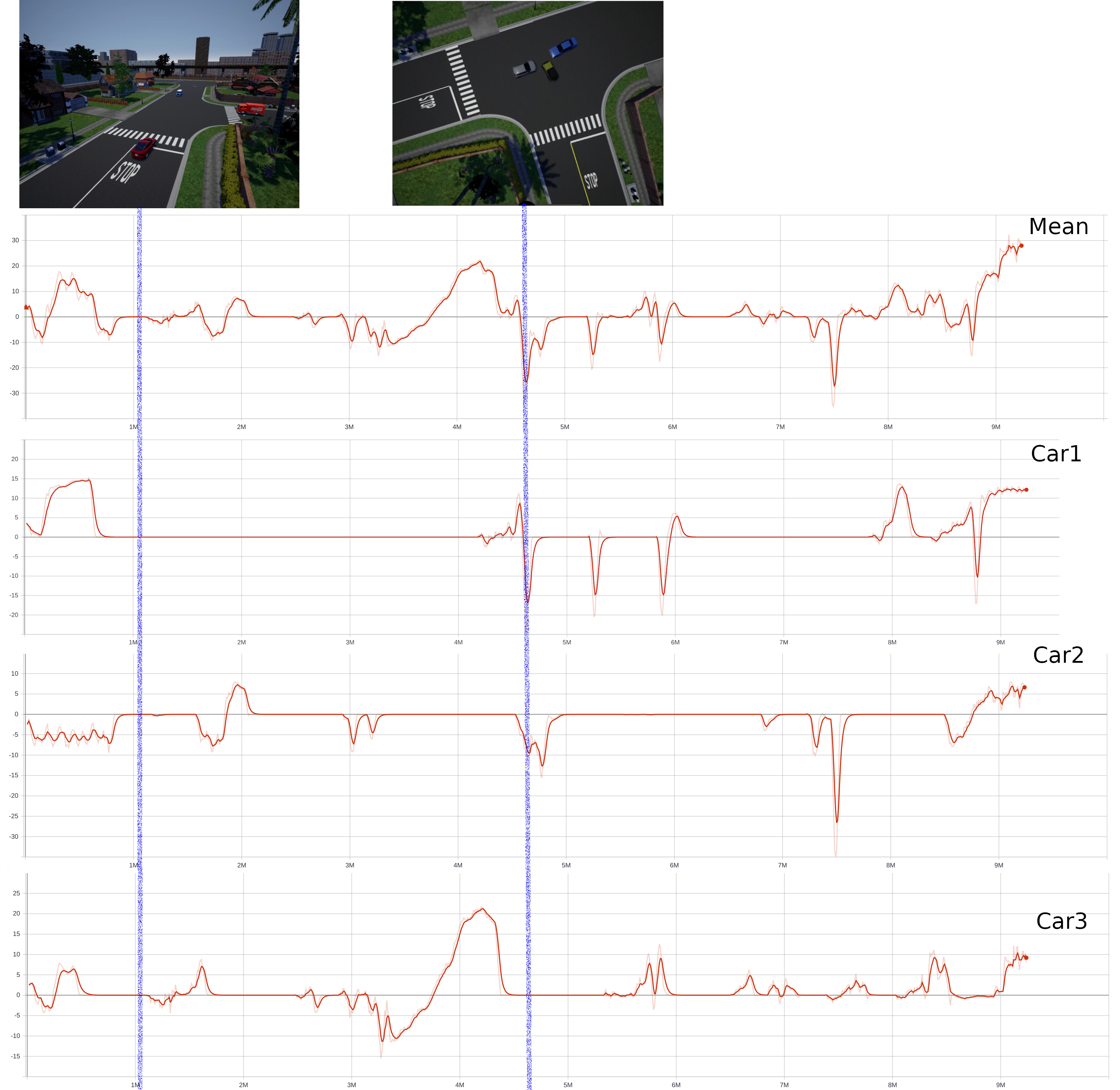
Figure 4: Figure shows the cumulative mean episodic rewards (legend:mean) and mean episodic rewards of car1 (legend:car1), car2 (legend:car2) and car3 (legend:car3). The blue vertical lines and the image at the top row indicate the states sampled during the corresponding training iteration (1.1M and 4.6M

.

C.4 Results

The performance of the multi-agent system is shown in Figure 4.

References

- Albrecht and Stone [2017] S. V. Albrecht and P. Stone. Autonomous Agents Modelling Other Agents: A Comprehensive Survey and Open Problems. arXiv e-prints, art. arXiv:1709.08071, Sep 2017.
- Brockman et al. [2016] G. Brockman, V. Cheung, L. Pettersson, J. Schneider, J. Schulman, J. Tang, and W. Zaremba. OpenAI Gym. arXiv e-prints, art. arXiv:1606.01540, Jun 2016.
- Chen et al. [2018] Y. Chen, P. Palanisamy, P. Mudalige, K. Muelling, and J. M. Dolan. Learning On-Road Visual Control for Self-Driving Vehicles with Auxiliary Tasks. arXiv e-prints, art. arXiv:1812.07760, Dec 2018.
- Dosovitskiy et al. [2017] A. Dosovitskiy, G. Ros, F. Codevilla, A. Lopez, and V. Koltun. CARLA: An Open Urban Driving Simulator. arXiv e-prints, art. arXiv:1711.03938, Nov 2017.
- Dulac-Arnold et al. [2019] G. Dulac-Arnold, D. Mankowitz, and T. Hester. Challenges of Real-World Reinforcement Learning. arXiv e-prints, art. arXiv:1904.12901, Apr 2019.
- El Sallab et al. [2017] A. El Sallab, M. Abdou, E. Perot, and S. Yogamani. Deep Reinforcement Learning framework for Autonomous Driving. arXiv e-prints, art. arXiv:1704.02532, Apr 2017.
- Emery-Montemerlo et al. [2004] R. Emery-Montemerlo, G. Gordon, J. Schneider, and S. Thrun. Approximate solutions for partially observable stochastic games with common payoffs. In Proceedings of the Third International Joint Conference on Autonomous Agents and Multiagent Systems - Volume 1, AAMAS ’04, pages 136–143, Washington, DC, USA, 2004. IEEE Computer Society. ISBN 1-58113-864-4. doi: 10.1109/AAMAS.2004.67. URL http://dx.doi.org/10.1109/AAMAS.2004.67.
- Espeholt et al. [2018] L. Espeholt, H. Soyer, R. Munos, K. Simonyan, V. Mnih, T. Ward, Y. Doron, V. Firoiu, T. Harley, I. Dunning, S. Legg, and K. Kavukcuoglu. IMPALA: Scalable Distributed Deep-RL with Importance Weighted Actor-Learner Architectures. arXiv e-prints, art. arXiv:1802.01561, Feb 2018.
- Foerster et al. [2016] J. N. Foerster, Y. M. Assael, N. de Freitas, and S. Whiteson. Learning to Communicate with Deep Multi-Agent Reinforcement Learning. arXiv e-prints, art. arXiv:1605.06676, May 2016.
- Hausknecht and Stone [2015] M. Hausknecht and P. Stone. Deep Recurrent Q-Learning for Partially Observable MDPs. arXiv e-prints, art. arXiv:1507.06527, Jul 2015.
- Horgan et al. [2018] D. Horgan, J. Quan, D. Budden, G. Barth-Maron, M. Hessel, H. van Hasselt, and D. Silver. Distributed Prioritized Experience Replay. arXiv e-prints, art. arXiv:1803.00933, Mar 2018.
- Isele et al. [2017] D. Isele, R. Rahimi, A. Cosgun, K. Subramanian, and K. Fujimura. Navigating Occluded Intersections with Autonomous Vehicles using Deep Reinforcement Learning. arXiv e-prints, art. arXiv:1705.01196, May 2017.
- Kendall et al. [2018] A. Kendall, J. Hawke, D. Janz, P. Mazur, D. Reda, J.-M. Allen, V.-D. Lam, A. Bewley, and A. Shah. Learning to Drive in a Day. arXiv e-prints, art. arXiv:1807.00412, Jul 2018.
- Kenney [2011] J. B. Kenney. Dedicated short-range communications (dsrc) standards in the united states. Proceedings of the IEEE, 99(7):1162–1182, July 2011. doi: 10.1109/JPROC.2011.2132790.
- Liang et al. [2017] E. Liang, R. Liaw, P. Moritz, R. Nishihara, R. Fox, K. Goldberg, J. E. Gonzalez, M. I. Jordan, and I. Stoica. RLlib: Abstractions for Distributed Reinforcement Learning. arXiv e-prints, art. arXiv:1712.09381, Dec 2017.
- Littman [1994] M. L. Littman. Markov Games As a Framework for Multi-agent Reinforcement Learning. ICML’94. Morgan Kaufmann Publishers Inc., San Francisco, CA, USA, 1994. ISBN 1-55860-335-2. URL http://dl.acm.org/citation.cfm?id=3091574.3091594.
- Lowe et al. [2017] R. Lowe, Y. Wu, A. Tamar, J. Harb, P. Abbeel, and I. Mordatch. Multi-Agent Actor-Critic for Mixed Cooperative-Competitive Environments. arXiv e-prints, art. arXiv:1706.02275, Jun 2017.
- Mnih et al. [2013] V. Mnih, K. Kavukcuoglu, D. Silver, A. Graves, I. Antonoglou, D. Wierstra, and M. Riedmiller. Playing Atari with Deep Reinforcement Learning. arXiv e-prints, art. arXiv:1312.5602, Dec 2013.
- Oliehoek [2012] F. A. Oliehoek. Decentralized pomdps. In Reinforcement Learning, pages 471–503. Springer, 2012.
- Panait and Luke [2005] L. Panait and S. Luke. Cooperative multi-agent learning: The state of the art. Autonomous Agents and Multi-Agent Systems, 11(3):387–434, Nov. 2005. ISSN 1387-2532. doi: 10.1007/s10458-005-2631-2. URL http://dx.doi.org/10.1007/s10458-005-2631-2.
- Qiao et al. [2018] Z. Qiao, K. Muelling, J. Dolan, P. Palanisamy, and P. Mudalige. Pomdp and hierarchical options mdp with continuous actions for autonomous driving at intersections. In 2018 21st International Conference on Intelligent Transportation Systems (ITSC), pages 2377–2382, Nov 2018. doi: 10.1109/ITSC.2018.8569400.
- SAE [2018] SAE. Taxonomy and Definitions for Terms Related to Driving Automation Systems for On-Road Motor Vehicles. Standard, Society of Automotive Engineers, June 2018.
- Shah et al. [2017] S. Shah, D. Dey, C. Lovett, and A. Kapoor. AirSim: High-Fidelity Visual and Physical Simulation for Autonomous Vehicles. arXiv e-prints, art. arXiv:1705.05065, May 2017.
- Shapley [1953] L. S. Shapley. Stochastic games. Proceedings of the National Academy of Sciences, 39(10):1095–1100, 1953. ISSN 0027-8424. doi: 10.1073/pnas.39.10.1095. URL https://www.pnas.org/content/39/10/1095.
- Tampuu et al. [2015] A. Tampuu, T. Matiisen, D. Kodelja, I. Kuzovkin, K. Korjus, J. Aru, J. Aru, and R. Vicente. Multiagent Cooperation and Competition with Deep Reinforcement Learning. arXiv e-prints, art. arXiv:1511.08779, Nov 2015.
- Udacity [2015] Udacity. Zero sum stochastic games two - georgia tech - machine learning, Feb 2015. URL https://www.youtube.com/watch?v=hsfEJEnNpJY.
- Wang et al. [2018] P. Wang, C.-Y. Chan, and A. de La Fortelle. A Reinforcement Learning Based Approach for Automated Lane Change Maneuvers. arXiv e-prints, art. arXiv:1804.07871, Apr 2018.
- Wikipedia [2019] Wikipedia. Cellular v2x, Jul 2019. URL https://en.wikipedia.org/wiki/Cellular_V2X.