The Equal-Time Quark Propagator in Coulomb Gauge

Abstract

We investigate the equal-time (static) quark propagator in Coulomb gauge within the Hamiltonian approach to QCD. We use a non-Gaussian vacuum wave functional which includes the coupling of the quarks to the spatial gluons. The expectation value of the QCD Hamiltonian is expressed by the variational kernels of the vacuum wave functional by using the canonical recursive Dyson–Schwinger equations (CRDSEs) derived previously. Assuming the Gribov formula for the gluon energy we solve the CRDSE for the quark propagator in the bare-vertex approximation together with the variational equations of the quark sector. Within our approximation the quark propagator is fairly insensitive to the coupling to the spatial gluons and its infrared behaviour is exclusively determined by the strongly infrared diverging instantaneous colour Coulomb potential.

I Introduction

Confinement and the spontaneous breaking of chiral symmetry leading to the dynamical generation of a constituent quark mass are the most important low-energy phenomena of Quantum Chromodynamics (QCD) at ordinary density and temperature. Research on this subject has been ongoing for decades (see Refs. [1, 2, 3, 4, 5, 6, 7] for some recent reviews) and various pictures have emerged, like the dual Meißner effect [8, 9], the center vortex scenario [10, 11, 12, 13, 14], and the Kugo–Ojima–Gribov–Zwanziger scenario [15, 16, 17, 18, 19]. Furthermore, these pictures are all supported by lattice calculations [20] and have been shown to be closely related [21, 22, 23]. Despite these efforts, a rigorous understanding of these phenomena is still lacking.

Much progress has been made in recent years using functional continuum methods like Dyson–Schwinger equations (DSEs) [1, 3, 4], Functional Renormalization Group (FRG) flow equations [2, 5], or variational methods in the Hamiltonian [24, 25, 18, 19, 26, 27, 28, 29, 30, 31, 32, 33] or Lagrange [34, 35] form. The variational approach has, in principle, the advantage over other continuum methods that it provides a criterium for the improvements of (the variational ansatz and) the truncations used. However, when one goes beyond Gaussian wave functionals one faces a problem: Wick’s theorem no longer applies, making a direct evaluation of expectation values in terms of the variational kernels of the vacuum wave functional impossible. In Refs [26, 29] this problem was elegantly solved using DSE techniques. The upshot is a set of DSE-like equations (named canonical recursive Dyson–Schwinger equations, CRDSEs) which relate the various $n$-point functions of the quark and gluon fields to the variational kernels of the vacuum wave functional. In the present paper we investigate the CRDSE for the (static) quark propagator.

The organization of the paper is as follows: In Sec. II we give a short summary of the Hamiltonian approach to QCD in Coulomb gauge developed in Ref. [29]. In Sec. III we discuss the truncation and renormalization scheme of the quark propagator CRDSE. The numerical input and the results are presented in Sec. IV, and some final remarks are given in Sec. V. In the Appendix we present the details of the infrared analysis of the relevant CRDSEs.

II Coulomb Gauge Equal-Time Quark Propagator

In terms of the fermion field operators $\psi$, $\psi^{\dagger}$ the equal-time quark propagator $S$ is defined by

$$S(1,2)\coloneq\frac{1}{2}\mathopen{}\mathclose{{}\left\langle\mathopen{\big{missing}}[\psi(1),\psi^{\dagger}(2)\mathclose{\big{missing}}]}\right\rangle.$$ (1)

We use here a condensed notation where a single numerical index stands collectively for the spatial coordinate and the colour and spinor indices. A repeated numerical label [see e.g. Eq. (3) later] implies integration over the spatial coordinate as well as summation over all discrete indices. Both the factor $1/2$ and the commutator on the right-hand side of Eq. (1) arise from the equal-time limit of the time-dependent propagator; the expectation value $\langle\ldots\rangle$ is taken in the ground state of the QCD Hamiltonian, which in Coulomb gauge takes the form [36]

$$\begin{split}H={}&\frac{1}{2}\int\mathop{}\!\mathrm{d}^{3}x\,J_{A}^{-1}E_{i}^{a}(\vx)J_{A}\,E_{i}^{a}(\vx)+\frac{1}{2}\int\mathop{}\!\mathrm{d}^{3}x\,B_{i}^{a}(\vx)\,B_{i}^{a}(\vx)\\ &+\int\mathop{}\!\mathrm{d}^{3}x\,\psi^{\dagger}(\vx)\bigl{[}-\mathrm{i}\mkern 1.0mu\valpha\cdot\grad-g\valpha\cdot\bm{\mathrm{A}}(\vx)+\beta m\bigr{]}\psi(\vx)\\ &+\frac{g^{2}}{2}\int\mathop{}\!\mathrm{d}^{3}x\mathop{}\!\mathrm{d}^{3}y\,J_{A}^{-1}\rho^{a}(\vx)\,J_{A}\,F_{A}^{ab}(\vx,\vy)\,\rho^{b}(\vy).\end{split}$$ (2)

Here, $E_{i}^{a}=\mathrm{i}\mkern 1.0mu\delta/\delta A_{i}^{a}$ and $B_{i}^{a}$ are the chromoelectric and -magnetic fields, $\alpha_{i}$ and $\beta$ are the usual Dirac matrices, $m$ is the bare current quark mass, and $\bm{\mathrm{A}}=\bm{\mathrm{A}}^{\!a\,}t^{a}$ are the (transverse) gauge fields with $t^{a}$ being the hermitian generators of the $\mathfrak{su}(N_{\mathrm{c}})$ algebra. The last term in Eq. (2) is the so-called Coulomb term: it describes the interaction of the colour charge density

$$\rho^{a}=\psi^{\dagger}\,t^{a}\psi-f^{abc}A_{i}^{b}\,E_{i}^{c}$$

through the Coulomb kernel

$$F_{A}(1,2)=G_{A}(1,3)\,G_{0}^{-1}(3,4)G_{A}(4,2),$$ (3)

where

$$G_{A}^{-1}(\vx,\vy)=\bigl{(}-\delta^{ab}\nabla^{2}_{x}-gf^{acb}A_{i}^{c}(\vx)\partial_{i}^{x}\bigr{)}\delta(\vx-\vy),\qquad G_{0}\equiv G_{A=0}$$

is the Faddeev–Popov operator of Coulomb gauge. Finally, $J_{A}=\operatorname{Det}G_{A}^{-1}$ is the corresponding Faddeev–Popov determinant.

For the fermionic operators $\psi$, $\psi^{\dagger}$ we use a representation based on coherent states $\lvert\xi\rangle$ (see Ref. [29] for details), where the action of $\psi$, $\psi^{\dagger}$ onto a fermionic state $\lvert\varPhi\rangle$ reads

$$\langle\xi\rvert\psi(1)\lvert\varPhi\rangle=\biggl{(}\xi_{-}(1)+\frac{\delta}{\delta\xi_{+}^{\dagger}(1)}\biggr{)}\varPhi[\xi],\qquad\langle\xi\rvert\psi^{\dagger}(1)\lvert\varPhi\rangle=\biggl{(}\xi_{+}^{\dagger}(1)+\frac{\delta}{\delta\xi_{-}(1)}\biggr{)}\varPhi[\xi].$$ (4)

In Eq. (4), $\varPhi[\xi]\equiv\langle\xi|\mathopen{}\varPhi\rangle$ is the coherent-state functional representation of the state $\lvert\varPhi\rangle$, and

$$\xi(1)=\xi_{+}(1)+\xi_{-}(1),\quad\xi_{\pm}(1)=\Lambda_{\pm}(1,2)\xi(2)$$

is a spinor-valued Grassmann field, with

$$\Lambda_{\pm}(1,2)=\int{\frac{\mathrm{d}^{3}p}{(2\pi)^{3}}}\mathop{}\!\mathrm{e}^{\mathrm{i}\mkern 1.0mu\vp\cdot(\vx_{1}-\vx_{2})}\Lambda_{\pm}(\vp),\qquad\Lambda_{\pm}(\vp)=\frac{1}{2}\pm\frac{\valpha\cdot\vp+\beta m}{2\sqrt{\vp^{2}+m^{2}}}$$ (5)

being the projectors onto positive/negative energy eigenstates of the free Dirac operator.

Denoting the ground state of the QCD Hamiltonian by $\varPsi[\xi,A]$, the vacuum expectation value $\langle O\rangle$ of an operator $O$ depending on both the gauge field $A$ and the fermionic fields $\psi^{\dagger}$, $\psi$ is given by the functional integral

$$\langle O\bigl{[}A,E,\psi,\psi^{\dagger}\bigr{]}\rangle=\int\mathcal{D}\xi^{\dagger}\,\mathcal{D}\xi\,\mathcal{D}A\,J_{A}\mathop{}\!\mathrm{e}^{-\mu}\,\varPsi^{*}[\xi,A]\,O\biggl{[}A,\mathrm{i}\frac{\delta}{\delta A},\xi_{-}+\frac{\delta}{\delta\xi_{+}^{\dagger}},\xi_{+}^{\dagger}+\frac{\delta}{\delta\xi_{-}}\biggr{]}\,\varPsi[\xi,A],$$ (6)

where

$$\mu=\xi^{\dagger}(1)\,S_{0}(1,2)\,\xi(2)$$

is the integration measure of the coherent fermion states, which involves the bare quark propagator

$$S_{0}(1,2)=\frac{1}{2}\bigl{[}\Lambda_{+}(1,2)-\Lambda_{-}(1,2)\bigr{]},\qquad S_{0}(\vp)=\frac{\valpha\cdot\vp+\beta m}{2\sqrt{\vp^{2}+m^{2}}}.$$ (7)

The vacuum wave functional $\varPsi[\xi,A]$ can be written as

$$\varPsi[\xi,A]\propto\exp\biggl{\{}-\frac{1}{2}\,S_{A}[A]-S_{f}[\xi,A]\biggr{\}},$$ (8)

where $S_{A}$ defines the vacuum wave functional of the pure Yang–Mills theory, while $S_{f}$ is the fermionic contribution, which includes also the coupling of the quarks to the spatial gluons. When all functional derivatives in Eq. (6) are worked out, expectation values of operators reduce to quantum averages of field functionals with an “action”

$$S=S_{A}+S_{f}+S_{f}^{*}+\mu.$$ (9)

This formal equivalence between vacuum expectation values in the Hamiltonian approach and functional integrals of a Euclidean field theory can be exploited to derive exact functional equations similar to Dyson–Schwinger equations [26, 29]. They differ from the standard DSEs in the sense that they do not connect propagators and vertices with the ordinary action but rather with the exponent of the vacuum wave functional. To stress the conceptual difference between the usual DSEs and the equations arising in our approach we named these ‘canonical recursive DSEs’ (CRDSEs).

The vacuum wave functional Eq. (8), and hence the action Eq. (9), is eventually determined by means of the variational principle: first we choose a suitable Ansatz for the vacuum wave functional, which depends on some variational kernels whose high-energy behaviour is known from perturbation theory [37, 38, 39, 40, 41], unless they are of non-perturbative origin. Then we evaluate the vacuum expectation value $\langle H\rangle$ of the Hamiltonian using the CRDSEs to relate the $n$-point functions appearing in $\langle H\rangle$ to the variational kernels of the vacuum wave functional. The resulting vacuum energy is then minimized with respect to the variational kernels. This procedure results in a set of gacoupledp equations for the variational kernels, which have to be solved together with the CRDSEs. The Ansatz chosen in Refs. [30, 32, 33] reads

$$S_{f}+S_{f}^{*}=\xi^{\dagger}(1)\,\bar{\gamma}(1,2)\,\xi(2)+\xi^{\dagger}(1)\,\bar{\Gamma}_{0}(1,2;3)\,\xi(2)A(3),$$

where the biquark kernel

$$\bar{\gamma}(1,2)=\Lambda_{+}(1,1^{\prime})\,K_{0}(1^{\prime},2^{\prime})\,\Lambda_{-}(2^{\prime},2)+\Lambda_{-}(1,1^{\prime})\,K_{0}^{\dagger}(1^{\prime},2^{\prime})\,\Lambda_{+}(2^{\prime},2)$$ (10)

and the bare quark-gluon vertex

$$\bar{\Gamma}_{0}(1,2;3)=\Lambda_{+}(1,1^{\prime})\,K(1^{\prime},2^{\prime};3)\,\Lambda_{-}(2^{\prime},2)+\Lambda_{-}(1,1^{\prime})\,K^{\dagger}(1^{\prime},2^{\prime};3)\,\Lambda_{+}(2^{\prime},2)$$ (11)

involve the variational kernels $K_{0}$ and $K$, for which we have chosen the form

$$K_{0}(\vp) =\beta s(\vp),$$ (12)

$$K_{i}^{a}(\vp,\vq;\vk) =gt^{a}\bigl{[}\alpha_{i}\,V(\vp,\vq)+\beta\alpha_{i}\,W(\vp,\vq)\bigr{]}(2\pi)^{3}\delta(\vp+\vq+\vk).$$ (13)

A more general form for $K_{0}$ could be chosen, but as shown in Ref. [33] the simple form Eq. (12) already captures the relevant physics. The variational kernel $K$ [Eq. (13)] contains a leading-order term involving the Dirac matrix $\alpha_{i}$ and a further contribution proportional to $\beta\alpha_{i}$. The latter term, introduced in Ref. [30], turns out to be of purely non-perturbative nature but is crucial to ensure one-loop renormalizability of the physical quark propagator [33]. In Refs. [30, 32, 33] the vacuum expectation value of the QCD Hamiltonian was calculated in the chiral limit $m=0$ up to including two-loop order, and the minimization with respect to the variational kernels resulted in four coupled equations for the scalar functions $s$, $V$, $W$, and the gluon energy $\Omega$. The equations for the vector kernels $V$ and $W$ can be explicitly solved in terms of the scalar kernel $s$ and the gluon energy $\Omega$, yielding

$$V(\vp,\vq) =-\frac{1+s_{p}s_{q}}{\Omega(\vp+\vq)+\lvert\vp\rvert\frac{1-s_{p}^{2}+2s_{p}s_{q}}{1+s_{p}^{2}}+\lvert\vq\rvert\frac{1-s_{q}^{2}+2s_{p}s_{q}}{1+s_{q}^{2}}},$$ (14a)

$$V(\vp,\vq) =-\frac{s_{p}-s_{q}}{\Omega(\vp+\vq)+\lvert\vp\rvert\frac{1-s_{p}^{2}-2s_{p}s_{q}}{1+s_{p}^{2}}+\lvert\vq\rvert\frac{1-s_{q}^{2}-2s_{p}s_{q}}{1+s_{q}^{2}}}.$$ (14b)

The scalar kernel $s_{p}$ itself obeys a gap equation (see Sec. III.2 later). The same is true for the gluon energy $\Omega$. It was shown in Ref. [30] that the unquenching of the gluon energy by the quarks is negligible. We will therefore use for $\Omega$ the Gribov formula, see Eq. (30) below, which nicely fits the lattice data for the gluon propagator in pure Yang–Mills theory.

As pointed out above, in the CRDSEs the variational kernels occurring in the vacuum wave functional [or, more exactly, their combinations Eqs. (10) and (11)] play the role of the bare vertices in the Lagrangian approach. We stress, however, that the word ‘bare’ means here leading-order in a skeleton expansion, and not lowest-order in perturbation theory. In fact, the scalar kernel $s_{p}$ and the vector kernel $W$ are identically zero in any order perturbation theory.

In terms of the fermionic fields $\xi$, $\xi^{\dagger}$, the physical quark propagator Eq. (1) reads

$$S(1,2)=\langle\xi(1)\,\xi^{\dagger}(2)\rangle-S_{0}(1,2)$$ (15)

where $S_{0}$ is the bare quark propagator Eq. (7). The additional term $S_{0}$ is a consequence of the chosen coherent-state representation, Eq. (4), of the fermion field operators. The quantity

$$Q(1,2)\equiv\langle\xi(1)\xi^{\dagger}(2)\rangle,$$ (16)

referred to as fermion propagator, obeys the CRDSE [29]

$$Q^{-1}(1,2)=\bigl{[}2S_{0}(1,2)\bigr{]}^{-1}+\bar{\gamma}(1,2)-\bar{\Gamma}_{0}(1,3;4)Q(3,3^{\prime})D(4,4^{\prime})\bar{\Gamma}(3^{\prime},2;4^{\prime}),$$ (17)

which is diagrammatically represented in Fig. 1.

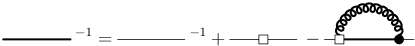
Figure 1: Diagrammatic representation of the CRDSE (17) for the quark propagator. Full lines and filled dots represent, respectively, dressed propagators and vertices. The line with an empty square stands for the biquark kernel $\bar{\gamma}$ [Eq. (10)]; the vertex with a square box represents the bare quark-gluon vertex $\bar{\Gamma}_{0}$ [Eq. (11)].

In Eq. (17), $S_{0}$ is the bare quark propagator Eq. (7),

$$D(1,2)=\langle A(1)A(2)\rangle$$ (18)

is the gluon propagator, and $\bar{\Gamma}$ is the full quark-gluon vertex defined by

$$\langle\xi(1)\xi^{\dagger}(2)A(3)\rangle=-Q(1,1^{\prime})\,\bar{\Gamma}(1^{\prime},2^{\prime};3^{\prime})\,Q(2^{\prime},2)\,D(3^{\prime},3).$$ (19)

The full quark-gluon vertex $\bar{\Gamma}$ also obeys a CRDSE, whose form is diagrammatically represented in Fig. 2.

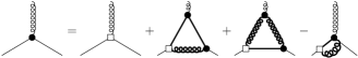
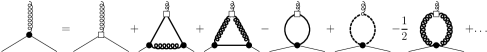
Figure 2: Possible forms of the CRDSE for the quark-gluon vertex with the bare vertex attached to the external quark (top) and gluon (bottom) leg. The ellipsis in the bottom figure stands for two-loop diagrams.

The leading term is given by $\bar{\Gamma}_{0}$ [Eq. (11)], thus justifying its interpretation as bare quark-gluon vertex.

Assuming a power law behaviour

$$Q(p)\overset{p\to 0}{\sim}\frac{1}{p^{\delta}},\qquad\bar{\Gamma}(p,p)\overset{p\to 0}{\sim}\frac{1}{p^{\eta}}$$ (20)

for the vertex and the propagator an IR analysis of the quark propagator CRDSE (17) leads to the condition (see the Appendix)

$$\delta=\min(0,5-\delta-\eta),$$

while the vertex CRDSE truncated to include only the triangle diagrams yields

$$\eta=\max(-1,2\eta+\delta-7,2\eta+2\delta-5).$$

Combining these two relations results in the following conditions for the IR exponents

$$\mathopen{}\mathclose{{}\left\{\begin{array}[]{@{}l@{}}\delta=0\\ \eta=-1\text{ or }5\end{array}}\right.\qquad\text{or}\qquad\mathopen{}\mathclose{{}\left\{\begin{array}[]{@{}l@{}}-2\leq\delta\leq 0\\ \eta=5-2\delta\end{array}}\right.$$

In the case of an IR constant quark propagator, $\delta=0$, the possible outcomes are $\eta=-1$ (i.e. IR suppressed quark-gluon vertex) and $\eta=5$. In view of the experience from FRG and DSE investigations in Landau gauge [44, 45, 46, 47, 48, 49, 50, 51, 52, 53, 54, 55, 56, 57] such a strongly IR divergent spatial vertex appears quite unlikely. We are confident that the solution with $\delta=0$ and $\eta=-1$ represents the physically realized case. For this solution the full quark-gluon vertex has the same infrared behaviour as the bare vertex.

III Truncation Scheme and Renormalization

III.1 Bare-Vertex Approximation

By global colour invariance the quark propagator has to be colour diagonal. For the inverse quark propagator we assume the following Dirac structure

$$Q^{-1}(\vp)=A(\vp)\,\valpha\cdot{\hat{\vp}}+\beta\,B(\vp).$$ (21)

In principle there might be further Dirac structures proportional to $\beta\alpha_{i}$ and $\mathbbm{1}$. However, from continuum studies [58] it is known that the term $\propto\beta\alpha_{i}$ cannot arise until two-loop order in perturbation theory. Furthermore, lattice simulations [59, 60] show no indication for the presence of such a structure. A term proportional to the unity matrix might well exist in the full (i.e. energy dependent) quark propagator but drops out when performing the energy integration required to obtain the static propagator. We will therefore stick to the form Eq. (21). With the explicit form of the biquark kernel Eq. (10) we obtain from the CRDSE (17) in the chiral limit the following system of coupled equations for the dressing functions $A$ and $B$ of the quark propagator Eq. (21)

$$\begin{split}A_{p}&=1-\frac{1}{4N_{\mathrm{c}}}\int{\frac{\mathrm{d}^{3}q}{(2\pi)^{3}}}\>\operatorname{tr}[\valpha\cdot{\hat{\vp}}\bar{\Gamma}_{0,i}^{mn,a}(\vp,-\vq;\vq-\vp)\,Q(\vq)\,D_{ij}(\vp-\vq)\,\bar{\Gamma}_{j}^{nm,a}(\vq,-\vp;\vp-\vq)],\\ B_{p}&=s_{p}-\frac{1}{4N_{\mathrm{c}}}\int{\frac{\mathrm{d}^{3}q}{(2\pi)^{3}}}\>\operatorname{tr}[\beta\bar{\Gamma}_{0,i}^{mn,a}(\vp,-\vq;\vq-\vp)\,Q(\vq)\,D_{ij}(\vp-\vq)\,\bar{\Gamma}_{j}^{nm,a}(\vq,-\vp;\vp-\vq)],\\ \end{split}$$ (22)

where the traces are taken over Dirac indices, and

$$D_{ij}(\vp)\equiv\frac{t_{ij}(\vp)}{2\Omega(\vp)},\qquad t_{ij}(\vp)=\delta_{ij}-\frac{p_{i}p_{j}}{\vp^{2}}$$

is the static gluon propagator Eq. (18), conveniently expressed by the quasi-gluon energy $\Omega(\vp)$.

Equation (22) still involves the full quark-gluon vertex $\bar{\Gamma}$ [Eq. (19)]. In the continuum QCD studies in Landau gauge both in the DSE and in the FRG approaches [44, 45, 46, 47, 48, 49, 50, 51, 52, 53, 54, 55, 56, 57] a non-perturbative dressing of the quark-gluon vertex is crucial to obtain spontaneous breaking of chiral symmetry. In Coulomb gauge the situation is different: chiral symmetry breaking is already triggered by the instantaneous colour Coulomb potential (see Sec. III.2) when the BCS-type wave functional is used for the quarks, i.e. when the vector kernels $V$ and $W$ in Eq. (13) are put to zero and thus the coupling of the quarks to the spatial gluons is disregarded. Furthermore, it was shown in Ref. [32] that for reasonable values of the strong coupling constant the inclusion of the coupling of the quarks to the spatial gluons influences only the high-momentum behaviour of the scalar kernel. Moreover, as shown above, bare and dressed quark-gluon vertices have the same IR behaviour. Therefore, in the following we replace the full quark-gluon vertex $\bar{\Gamma}$ by the bare one $\bar{\Gamma}_{0}$ [Eq. (11)]. We will discuss the quality of this approximation later. After replacing the full vertices in the CRDSE (22) by bare ones, the Dirac traces can be worked out and the coupled equations (22) for the dressing functions of the quark propagator reduce to

$$A_{p} =1+\frac{g^{2}C_{F}}{2}\int{\frac{\mathrm{d}^{3}q}{(2\pi)^{3}}}\>\frac{A_{q}}{\Omega(\vp+\vq)\,\Delta_{q}}\biggl{[}X_{-}(\vp,\vq)\,V^{2}(\vp,\vq)+X_{+}(\vp,\vq)\,W^{2}(\vp,\vq)\biggr{]}\equiv 1+I_{A},$$ (23a)

$$B_{p} =s_{p}+\frac{g^{2}C_{F}}{2}\int{\frac{\mathrm{d}^{3}q}{(2\pi)^{3}}}\,\frac{B_{q}}{\Omega(\vp+\vq)\,\Delta_{q}}\biggl{[}X_{-}(\vp,\vq)\,V^{2}(\vp,\vq)-X_{+}(\vp,\vq)\,W^{2}(\vp,\vq)\biggr{]},$$ (23b)

where $C_{F}=(\mathrlap{N_{\mathrm{c}}}N_{\hphantom{\mathrm{c}}}^{2}-1)/(2N_{\mathrm{c}})$ is the Casimir eigenvalue in the fundamental representation,

$$\Delta_{p}=A_{p}^{2}+B_{p}^{2},$$

and the factors

$$X_{\pm}(\vp,\vq)=1\pm\frac{[{\hat{\vp}}\cdot(\vp+\vq)][{\hat{\vq}}\cdot(\vp+\vq)]}{(\vp+\vq)^{2}}$$

arise from the contraction of the trace of Dirac matrices with the transverse projector $t_{ij}(\vp)$.

III.2 The Biquark Kernel

In principle we should solve the two CRDSEs (23) with the vector kernels $V$ and $W$ [Eq. (14)] together with the gap equation for the scalar kernel $s_{p}$ derived in Refs. [30, 32, 33]. However, these previous investigations have shown that the effect of the spatial gluons on the scalar kernel $s_{p}$ is rather small. For physical values of the coupling $g$, the scalar kernel is dominated by the strongly IR divergent colour Coulomb potential: in particular the IR behaviour of $s_{p}$ is exclusively determined by the Coulomb term. Therefore, in the following we assume that the scalar kernel $s_{p}$ satisfies the gap equation obtained without the coupling to the spatial gluons, which is given by

$$\lvert\vp\rvert\,s_{p}=\frac{g^{2}C_{F}}{2}\int{\frac{\mathrm{d}^{3}q}{(2\pi)^{3}}}\,F(\vp-\vq)\,\frac{s_{q}(1-s_{p}^{2})-{\hat{\vp}}\cdot{\hat{\vq}}\,s_{p}(1-s^{2}_{q})}{1+s_{q}^{2}}.$$ (24)

Here, the colour Coulomb potential $F(\vp)$ is the expectation value of the Coulomb kernel Eq. (3). Previous studies [69, 70, 19, 23] show that in coordinate space the expectation value of $F_{A}$ raises linearly for large distances. In fact, an IR analysis of the variational equations of the Yang–Mills sector reveals the IR behaviour

$$g^{2}F(\vp)=\frac{8\pi\sigma_{\mathrm{C}}}{(\vp^{2})^{2}},$$ (25)

where $\sigma_{\mathrm{C}}$ is the Coulomb string tension: $\sigma_{\mathrm{C}}$ is larger than the Wilson string tension $\sigma$ by a factor ranging from 2.5 to 4 [71, 72, 73], the latter value seemingly being favoured by recent lattice calculations [74]. In the numerical solution of Eq. (24) we use the IR from Eq. (25) of the Coulomb propagator and set $\sigma_{\mathrm{C}}\simeq 4\sigma$, fixing our scale at $\sqrt{\sigma_{\mathrm{C}}}=0.88\,\mathrm{GeV}$. For numerical reasons the gap equation (24) is reformulated in terms of the mass function $m_{p}$

$$m_{p}=\frac{2ps_{p}}{1-s_{p}^{2}}\quad\Rightarrow\quad s_{p}=\sqrt{1+p^{2}/m_{p}^{2}}-p/m_{p},$$ (26)

resulting in

$$m_{p}=\frac{g^{2}C_{F}}{2}\int{\frac{\mathrm{d}^{3}q}{(2\pi)^{3}}}\frac{F(\vp-\vq)}{\sqrt{\vq^{2}+m_{q}^{2}}}\biggl{[}m_{q}-\frac{\vp\cdot\vq}{\vp^{2}}\,m_{p}\biggr{]}.$$ (27)

The numerical solution [75] of the gap equation Eq. (27) can be fitted by

$$m_{p}=\frac{0.19099\sqrt{\sigma_{\mathrm{C}}}}{\bigl{[}1+0.95086\bigl{(}p/\sqrt{\sigma_{\mathrm{C}}}\bigr{)}{}^{1.7648}\bigr{]}^{2.6632}}.$$ (28)

Figure 3 shows the numerical solution of the gap equation (27) together with the fit Eq. (28).

Figure 3: Numerical solution of the gap equation (27) together with the fit Eq. (28).

III.3 Renormalization and Chiral Condensate

The equation (23a) for the dressing function $A_{p}$ is UV divergent. Using a sharp UV cut-off we find

$$A_{p}=1+\frac{\alpha_{s}C_{F}}{4\pi}(1+s_{p}^{2})\ln\Lambda+\text{finite terms}$$

where $\alpha_{s}=g^{2}/(4\pi)$ is the strong coupling constant. As we have shown in Ref. [33], the occurrence of a momentum-dependent divergence poses no conceptual problem, since $A_{p}$ and $B_{p}$ are the dressing functions of the propagator $Q$ [Eq. (16)] of the coherent-state fields $\xi$, $\xi^{\dagger}$ and not of the physical quark propagator $S$ [Eqs. (1) and (15)]. We renormalize the equation for $A_{p}$ by subtracting it at an arbitrary scale $\mu$, obtaining

$$A_{p}=1+\frac{1+s_{p}^{2}}{1+s_{\mu}^{2}}(A_{\mu}-1)+\lim_{\Lambda\to\infty}\biggl{[}I_{A}(p,\Lambda)-\frac{1+s_{p}^{2}}{1+s_{\mu}^{2}}\,I_{A}(\mu,\Lambda)\biggr{]},$$ (29)

where $I_{A}$ is the loop integral on the right-hand side of Eq. (23a).

Once the results for $A_{p}$ and $B_{p}$ are known, the chiral condensate can be evaluated by

$$\langle\bar{q}q\rangle=-\frac{2N_{\mathrm{c}}}{\pi^{2}}\int\mathop{}\!\mathrm{d}p\,p^{2}\frac{B_{p}}{A_{p}^{2}+B_{p}^{2}}.$$

IV Results

We have solved the coupled equations (23b) and (29) with the variational kernels $V$ [Eq. (14a)], $W$ [Eq. (14b)] and $s_{p}$ [Eq. (26)] calculated from the solution Eq. (28) of the gap equation (24). The quasi-gluon energy $\Omega$ is parametrized by the Gribov formula [15, 76]

$$\Omega(\vp)=\sqrt{\vp^{2}+m_{A}^{4}/\vp^{2}}.$$ (30)

For the Gribov mass $m_{A}$ we have taken the value

$$m_{A}^{2}=\frac{N_{\mathrm{c}}}{\pi}\,\sigma_{\mathrm{C}}$$

resulting from the IR analysis of the gluon gap equation [19]. The results are shown in Fig. 4 in a MOM scheme with $A_{\mu}=1$ for the renormalization scale $\mu=2\,\mathrm{GeV}$. The value $\alpha_{s}(2\,\mathrm{GeV})=0.30(1)$ [77] in the $\overline{\text{MS}}$ scheme can be converted to the MOM value $\alpha_{s}^{\mathrm{MOM}}(2\,\mathrm{GeV})\simeq 0.44$ by means of the three-loop $\beta$ function [78].

(a)

(b)

Figure 4: Dressing functions $A_{p}$ and $B_{p}$ of the fermion propagator Eq. (16) renormalized at $\mu=2\,\mathrm{GeV}$ (left panel) and of the physical quark propagator Eq. (31) (right panel). The curves labelled ‘no coupling’ refer to the case where the coupling to the spatial gluons is ignored, iwhich results in $A_{p}=1$ and $B_{p}=s_{p}$.

Figure 4a shows the dressing functions $A_{p}$ and $B_{p}$ of the fermion propagator Eq. (16) together with the values $A_{p}=1$ and $B_{p}=s_{p}$ which follow when the coupling to the spatial gluons is ignored. The physical quark propagator Eq. (15) becomes in momentum space

$$S(\vp)=Q(\vp)-S_{0}(\vp)=\frac{A_{p}\valpha\cdot{\hat{\vp}}+B_{p}\beta}{A_{p}^{2}+B_{p}^{2}}-\frac{\valpha\cdot{\hat{\vp}}}{2}\equiv f_{\alpha}(p)\valpha\cdot{\hat{\vp}}+f_{\beta}(p)\beta.$$ (31)

with dressing functions

$$f_{\alpha}(p)=\frac{A_{p}}{A_{p}^{2}+B_{p}^{2}}-\frac{1}{2},\qquad f_{\beta}(p)=\frac{B_{p}}{A_{p}^{2}+B_{p}^{2}},$$

which are shown in Fig. 4b. The dressing function $f_{\alpha}$ of the $\alpha_{i}$ piece of the propagator develops an anomalous dimension in the UV, compatible with the perturbative analysis [41].

For the chiral condensate we recover the value $(-236\,\mathrm{MeV})^{3}$. Both the dressing functions of the physical quark propagator and the chiral condensate differ only little from the values obtained by ignoring the coupling to the spatial gluons and from the one-loop expansion of Ref. [33].

V Conclusions

We have solved numerically the CRDSEs for the quark propagator under the assumptions that i) the scalar kernel is dominated by the IR diverging colour Coulomb interactions, and ii) that we can replace the full quark-gluon vertex by the bare one. While we are very confident that the first assumption is reliable, the second one is less under control. It is well-known from Landau gauge studies [44, 45, 46, 47, 48, 49, 50, 51, 52, 53, 54, 55, 56, 57] that a number of Dirac structures beyond the leading order $\gamma^{\mu}$ contribute to the overall strength of the vertex. The quark-gluon vertex in Coulomb gauge is currently under investigation. It is more involved than its Landau-gauge counterpart: because of the projectors Eq. (5) in Eq. (11), the bare vertex alone involves five different Dirac structures instead of one. Furthermore, since the Coulomb gauge is non-covariant the total number of Dirac structures must be nearly doubled, because the temporal and spatial Dirac matrices must be treated separately. It is very likely that all these further tensor structures appearing in the full vertex are not as relevant as in Landau gauge; this is because in our approach chiral symmetry breaking is caused by the Coulomb term and not by the quark-gluon vertex as it is the case in Landau gauge. Keeping only this dominant contribution could be a useful phenomenological tool for further calculations at finite temperature and density.

Appendix A Infrared Analysis

Suppressing all indices, the fermion propagator CRDSE (17) can be written as

$$Q^{-1}=\bigl{[}2S_{0}\bigr{]}^{-1}+\bar{\gamma}+\int\bar{\Gamma}Q\bar{\Gamma}_{0}D.$$ (32)

The IR analysis is performed in the usual way by rescaling all momenta by a factor $\lambda$, $\vp\to\lambda\vp$ and $\vq\to\lambda\vq$, sending $\lambda\to 0$, replacing the various Green functions by their assumed IR scaling behaviour [Eq. (20)], and comparing the powers of $\lambda$. The biquark kernel $\bar{\gamma}$ [Eqs. (10) and (12)] and the bare quark propagator $S_{0}$ [Eq. (7)] are IR constant

$$\bar{\gamma}\sim S_{0}\sim\lambda^{0}$$

while the bare quark-gluon vertex [Eqs. (11) and (13)] vanishes in the IR because of the IR diverging gluon energy $\Omega$ [Eq. (30)] in the denominator of the vector kernels $V$ and $W$ [Eqs. (14)]

$$\bar{\Gamma}_{0}\sim\lambda.$$

From Eq. (32) we find with a factor $\lambda^{3}$ coming from the momentum integration:

$$\lambda^{\delta}\sim\lambda^{0}+\lambda^{3-\eta-\delta+1+1}.$$

For $\lambda\to 0$ the smaller exponent dominates, and we obtain

$$\delta=\min(0,5-\delta-\eta).$$

For the IR analysis of the CRDSE for the quark-gluon vertex we choose the equation with the bare vertex attached to the external gluon leg (second equation in Fig. 2) and keep only the triangle diagrams. This CRDSE then becomes

$$\bar{\Gamma}=\bar{\Gamma}_{0}+\int\bar{\Gamma}Q\bar{\Gamma}_{0}Q\bar{\Gamma}D+\int\bar{\Gamma}Q\bar{\Gamma}D^{2}\gamma_{3}$$ (33)

where $\gamma_{3}$ is the three-gluon kernel determined in Ref. [26]. The latter vanishes as $\lambda^{2}$ for $\lambda\to 0$. From the CRDSE (33) we find

$$\lambda^{-\eta}\sim\lambda+\lambda^{3-\eta-\delta+1-\delta-\eta+1}+\lambda^{3-\eta-\delta-\eta+2+2}$$

resulting in

$$-\eta=\min(1,5-2\delta-2\eta,7-2\eta-\delta).$$

Using the version of the CRDSE with the bare vertex attached to the incoming quark line (first equation in Fig. 2) forces one to consider also the full three-gluon vertex, which was investigated in Ref. [79]. However, the conclusions presented at the end of Sec. II remain unaltered.

A possibly strong IR enhancement might come from the quark four-point function (see Fig. 2 bottom). Even if our vacuum wave functional Eq. (8) does not involve a four-point function, we can nevertheless try to estimate its effect: if we had such a term in our Ansatz, its leading-order expansion would be of the form

$$\bar{\Gamma}_{0,4q}\sim F+\bar{\Gamma}_{0,i}\bar{\Gamma}_{0,i}$$

where $F$ is the Coulomb propagator Eq. (25). Even with an IR exponent of $-4$ from the Coulomb propagator the whole diagram would not change the results of the IR analysis.

References

- [1] R. Alkofer and L. von Smekal, Phys. Rept. 353, 281 (2001), arXiv:hep-ph/0007355.
- [2] J. M. Pawlowski, Annals Phys. 322, 2831 (2007), arXiv:hep-th/0512261.
- [3] C. S. Fischer, J. Phys. G32, R253 (2006), arXiv:hep-ph/0605173.
- [4] D. Binosi and J. Papavassiliou, Phys. Rept. 479, 1 (2009), arXiv:0909.2536.
- [5] J. Braun, J. Phys. G39, 033001 (2012), arXiv:1108.4449.
- [6] G. Eichmann, H. Sanchis-Alepuz, R. Williams, R. Alkofer, and C. S. Fischer, Prog. Part. Nucl. Phys. 91, 1 (2016), arXiv:1606.09602.
- [7] S. Aoki et al., Eur. Phys. J. C77, 112 (2017), arXiv:1607.00299.
- [8] Y. Nambu, Phys. Rev. D10, 4262 (1974).
- [9] G. ’t Hooft, Nucl. Phys. B190, 455 (1981).
- [10] G. Mack and V. B. Petkova, Annals Phys. 123, 442 (1979).
- [11] H. B. Nielsen and P. Olesen, Nucl. Phys. B160, 380 (1979).
- [12] L. Del Debbio, M. Faber, J. Giedt, J. Greensite, and S. Olejnik, Phys. Rev. D58, 094501 (1998), arXiv:hep-lat/9801027.
- [13] K. Langfeld, H. Reinhardt, and O. Tennert, Phys. Lett. B419, 317 (1998), arXiv:hep-lat/9710068.
- [14] M. Engelhardt, K. Langfeld, H. Reinhardt, and O. Tennert, Phys. Rev. D61, 054504 (2000), arXiv:hep-lat/9904004.
- [15] V. Gribov, Nucl. Phys. B139, 1 (1978).
- [16] T. Kugo and I. Ojima, Prog. Theor. Phys. Suppl. 66, 1 (1979).
- [17] D. Zwanziger, Nucl. Phys. B518, 237 (1998).
- [18] C. Feuchter and H. Reinhardt, Phys. Rev. D70, 105021 (2004), arXiv:hep-th/0408236.
- [19] D. Epple, H. Reinhardt, and W. Schleifenbaum, Phys. Rev. D75, 045011 (2007), arXiv:hep-th/0612241.
- [20] J. Greensite, Lect. Notes Phys. 821, 1 (2011).
- [21] J. Greensite, S. Olejnik, and D. Zwanziger, JHEP 05, 070 (2005), arXiv:hep-lat/0407032.
- [22] H. Reinhardt, Phys. Rev. Lett. 101, 061602 (2008), arXiv:0803.0504.
- [23] G. Burgio, M. Quandt, H. Reinhardt, and H. Vogt, Phys. Rev. D92, 034518 (2015), arXiv:1503.09064.
- [24] D. Schutte, Phys. Rev. D31, 810 (1985).
- [25] A. P. Szczepaniak and E. S. Swanson, Phys. Rev. D65, 025012 (2001), arXiv:hep-ph/0107078.
- [26] D. R. Campagnari and H. Reinhardt, Phys. Rev. D82, 105021 (2010), arXiv:1009.4599.
- [27] M. Pak and H. Reinhardt, Phys. Lett. B707, 566 (2012), arXiv:1107.5263.
- [28] M. Pak and H. Reinhardt, Phys. Rev. D88, 125021 (2013), arXiv:1310.1797.
- [29] D. R. Campagnari and H. Reinhardt, Phys. Rev. D92, 065021 (2015), arXiv:1507.01414.
- [30] P. Vastag, H. Reinhardt, and D. Campagnari, Phys. Rev. D93, 065003 (2016), arXiv:1512.06733.
- [31] H. Reinhardt and P. Vastag, Phys. Rev. D94, 105005 (2016), arXiv:1605.03740.
- [32] D. R. Campagnari, E. Ebadati, H. Reinhardt, and P. Vastag, Phys. Rev. D94, 074027 (2016), arXiv:1608.06820.
- [33] D. Campagnari and H. Reinhardt, Phys. Rev. D97, 054027 (2018), arXiv:1801.02045.
- [34] M. Quandt, H. Reinhardt, and J. Heffner, Phys. Rev. D89, 065037 (2014), arXiv:1310.5950.
- [35] M. Quandt and H. Reinhardt, Phys. Rev. D92, 025051 (2015), arXiv:1503.06993.
- [36] N. H. Christ and T. D. Lee, Phys. Rev. D22, 939 (1980).
- [37] P. Mansfield, M. Sampaio, and J. Pachos, Int. J. Mod. Phys. A13, 4101 (1998), arXiv:hep-th/9702072.
- [38] P. Mansfield and M. Sampaio, Nucl. Phys. B545, 623 (1999), arXiv:hep-th/9807163.
- [39] D. R. Campagnari, H. Reinhardt, and A. Weber, Phys. Rev. D80, 025005 (2009), arXiv:0904.3490.
- [40] D. Campagnari, A. Weber, H. Reinhardt, F. Astorga, and W. Schleifenbaum, Nucl. Phys. B842, 501 (2011), arXiv:0910.4548.
- [41] D. R. Campagnari and H. Reinhardt, Int. J. Mod. Phys. A30, 1550100 (2015), arXiv:1404.2797.
- [42] R. Floreanini and R. Jackiw, Phys. Rev. D37, 2206 (1988).
- [43] C. Kiefer and A. Wipf, Annals Phys. 236, 241 (1994), arXiv:hep-th/9306161.
- [44] R. Alkofer, C. S. Fischer, F. J. Llanes-Estrada, and K. Schwenzer, Annals Phys. 324, 106 (2009), arXiv:0804.3042.
- [45] A. Aguilar and J. Papavassiliou, Phys. Rev. D83, 014013 (2011), arXiv:1010.5815.
- [46] D. Binosi, L. Chang, J. Papavassiliou, S.-X. Qin, and C. D. Roberts, Phys. Rev. D95, 031501 (2017), arXiv:1609.02568.
- [47] A. C. Aguilar, D. Binosi, D. Ibañez, and J. Papavassiliou, Phys. Rev. D90, 065027 (2014), arXiv:1405.3506.
- [48] A. C. Aguilar, J. C. Cardona, M. N. Ferreira, and J. Papavassiliou, Phys. Rev. D96, 014029 (2017), arXiv:1610.06158.
- [49] A. C. Aguilar, J. C. Cardona, M. N. Ferreira, and J. Papavassiliou, Phys. Rev. D98, 014002 (2018), arXiv:1804.04229.
- [50] M. Mitter, J. M. Pawlowski, and N. Strodthoff, Phys. Rev. D91, 054035 (2015), arXiv:1411.7978.
- [51] J. Braun, L. Fister, J. M. Pawlowski, and F. Rennecke, Phys. Rev. D94, 034016 (2016), arXiv:1412.1045.
- [52] A. K. Cyrol, M. Mitter, J. M. Pawlowski, and N. Strodthoff, Phys. Rev. D97, 054006 (2018), arXiv:1706.06326.
- [53] A. Windisch, M. Hopfer, and R. Alkofer, (2012), arXiv:1210.8428, [Acta Phys. Polon. Supp.6,347(2013)].
- [54] R. Williams, C. S. Fischer, and W. Heupel, Phys. Rev. D93, 034026 (2016), arXiv:1512.00455.
- [55] H. Sanchis-Alepuz and R. Williams, Phys. Lett. B749, 592 (2015), arXiv:1504.07776.
- [56] O. Oliveira, T. Frederico, W. de Paula, and J. P. B. C. de Melo, Eur. Phys. J. C78, 553 (2018), arXiv:1807.00675.
- [57] O. Oliveira, W. de Paula, T. Frederico, and J. P. B. C. de Melo, Eur. Phys. J. C79, 116 (2019), arXiv:1807.10348.
- [58] P. Watson and H. Reinhardt, Phys. Rev. D85, 025014 (2012), arXiv:1111.6078, 27 pages, 11 figures.
- [59] G. Burgio, M. Schrock, H. Reinhardt, and M. Quandt, Phys. Rev. D86, 014506 (2012), arXiv:1204.0716.
- [60] M. Pak and M. Schröck, Phys. Rev. D91, 074515 (2015), arXiv:1502.07706.
- [61] J. Finger, D. Horn, and J. Mandula, Phys. Rev. D20, 3253 (1979).
- [62] J. R. Finger and J. E. Mandula, Nucl. Phys. B199, 168 (1982).
- [63] A. Amer, A. Le Yaouanc, L. Oliver, O. Pene, and J. c. Raynal, Phys. Rev. Lett. 50, 87 (1983).
- [64] A. Le Yaouanc, L. Oliver, O. Pene, and J. C. Raynal, Phys. Rev. D29, 1233 (1984).
- [65] S. L. Adler and A. Davis, Nucl. Phys. B244, 469 (1984).
- [66] A. C. Davis and A. M. Matheson, Nucl. Phys. B246, 203 (1984).
- [67] R. Alkofer and P. Amundsen, Nucl. Phys. B306, 305 (1988).
- [68] P. J. d. A. Bicudo and J. E. F. T. Ribeiro, Phys. Rev. D42, 1611 (1990).
- [69] D. Zwanziger, Phys. Rev. Lett. 90, 102001 (2003), arXiv:hep-lat/0209105.
- [70] D. Zwanziger, Phys. Rev. D70, 094034 (2004), arXiv:hep-ph/0312254.
- [71] Y. Nakagawa, A. Nakamura, T. Saito, H. Toki, and D. Zwanziger, Phys. Rev. D73, 094504 (2006), arXiv:hep-lat/0603010.
- [72] M. Golterman, J. Greensite, S. Peris, and A. P. Szczepaniak, Phys. Rev. D85, 085016 (2012), arXiv:1201.4590.
- [73] J. Greensite and A. P. Szczepaniak, Phys. Rev. D91, 034503 (2015), arXiv:1410.3525.
- [74] J. Greensite and A. P. Szczepaniak, Phys. Rev. D93, 074506 (2016), arXiv:1505.05104.
- [75] M. Quandt, E. Ebadati, H. Reinhardt, and P. Vastag, Phys. Rev. D98, 034012 (2018), arXiv:1806.04493.
- [76] G. Burgio, M. Quandt, and H. Reinhardt, Phys. Rev. Lett. 102, 032002 (2009), arXiv:0807.3291.
- [77] A. Buckley et al., Eur. Phys. J. C75, 132 (2015), arXiv:1412.7420.
- [78] K. G. Chetyrkin and T. Seidensticker, Phys. Lett. B495, 74 (2000), arXiv:hep-ph/0008094.
- [79] M. Q. Huber, D. R. Campagnari, and H. Reinhardt, Phys. Rev. D91, 025014 (2015), arXiv:1410.4766.