Photometric reverberation mapping of AGNs at $0.1<z<0.8$: I.
Observational technique

Abstract

The improvement of the calibration relation for determining the size of the broad-line region from the observed optical luminosity of active galactic nuclei (AGN) is a necessary task to study fundamental parameters of distant AGNs such as mass of the central supermassive black hole. The most popular method of the BLR size estimation is the reverberation mapping based on measuring the time delay between the continuum flux and the flux in the emission lines. In our work, we apply the method of photometric reverberation mapping in medium-band filters, adapted for observations at the Zeiss-1000 telescope of the SAO RAS, for the study of AGN with broad lines in the range of redshifts $0.1<z<0.8$. This paper describes the technique of observations and data processing, provides a sample of objects and demonstrates the stability of the used method. As a preliminary result for 2MASX J08535955+7700543 at $z=0.1$ we have obtained time delay estimates of $\tau(ICCF)=32.2^{\pm 10.6}$ days and $\tau({\rm JAVELIN})=39.5_{-15.8}^{+23.0}$ days that are consistent with each other and also within the accuracy of the existing calibration relations.

Received: December 26, 2018.  Accepted: September 23, 2019.

I Introduction

According to modern concepts, in the centers of most massive galaxies, there are supermassive black holes (SMBH) weighing from a million to tens of billions of solar masses. In the active galactic nuclei (AGN), the accretion of gas onto a supermassive black hole leads to the release of a huge amount of energy. Variable accretion disc radiation in the ultraviolet part of the spectrum ionizes gas clouds in the broad-line region (BLR), which then re-emit energy in the emission lines due to photorecombination. The reverberation mapping method (RM) consists in measuring the time delay $\tau$ between the radiation of the accretion disk responsible for the formation of the continuum and the radiation in the emission lines produced in the BLR region BlanfordMKee82 . It is assumed that the size of the BLR $R_{\rm BLR}\equiv c\tau$, where $c$ is the speed of light Peterson93 . Then $R_{\rm BLR}$ can be determined by measuring the time lag $\tau$ of the light curve in an emission line relative to the one in the continuum associated by an integral transformation with the cross-correlation function kernel.

The first works on the measurement of the time delay $\tau$ between H_α and the ultraviolet continuum radiation in galaxies with active nuclei were carried out in the paper by Cherepashchuk and Lyutyi in 1973 CherepLyut73 . For the investigating galaxies NGC 4151, NGC 3516 and NGC 1068 the delays were found—30, 25 and 15 days, respectively, which gives the BLR size $c\tau$ $\sim$ 0.02 pc. Reverberation mapping method was developed in several papers (e.g., BlanfordMKee82 ; AntBoch83 ; GaskellSparke86 and others).

The data on the BLR size gained for AGNs by RM during the previous 15 years were collected and analyzed in the paper by Peterson et al. Peterson04 . The paper by Bentz and Katz 2015 BentzKatz15 describes a database with a compilation of all published at that time 63 AGNs with the estimation of central black holes masses. However, the database BentzKatz15 contains observational data only for the nearest AGNs up to $z\sim 0.3$ as well as many later RM investigations (e.g. Du16 ; Jiang16 ; Nunez17 ).

RM of distant AGNs is particularly interesting. Since the gas dynamics in the BLR is influenced by the SMBH gravitation, according to the virial ratio its mass is related to the size $c\tau$ and the gas velocity in the BLR $\upsilon_{\rm line}$ as:

$$M_{\rm SMBH}=fc\tau\upsilon_{\rm line}^{2}G^{-1},$$

where $G$ is the gravitational constant, $c$ is the speed of light, $f$ is a dimensionless factor of the order of one depending on the BLR structure and kinematics and the angle of the system inclination relative to the observer.

Thus, the extension of the AGN sample with known sizes $R_{\rm BLR}$ to more distant redshifts will allow one to trace the evolution of the SMBH masses. The largest campaign of BLR RM at bigger $z$ is the SDSS-RM project Shen15 monitoring 849 quasars with broad lines in the range of the redshifts $0.1<z<4.5$. SDSS-RM collaboration presents the first results of measurements of the time delays for 44 and 18 quasars using H_β and H_α lines, respectively, in the $0.11<z<1.13$ range Grier17 ; Grier18err . It is also noted that for distant objects, it is needed to observe the delay $\tau$ in the lines with higher ionization potentials that are in a shorter wavelength part of the spectrum compared to the Balmer series. For these purposes, such lines as Mg II could be used (2798 Å) (Czerny19 and references therein).

However, the RM method requires the accumulation of a long series of observational data making harder its wide application. It has been observed that for active nuclei there is a relation between the BLR size and AGN luminosity: $R_{\rm BLR}\propto L^{\alpha}$. Currently, several empirical relations are linking the size $R_{\rm BLR}$ obtained by measuring the delay in different lines and luminosity in different spectral bands. The most popular relation used for nearest objects is $R_{\rm BLR}-L_{\lambda}$ (5100 Å), where $R_{\rm BLR}$ is the BLR size measured by the radiation delay in the line H_β, and $L_{\lambda}$ (5100 Å) is the luminosity of the AGN in the range 4400–5850 Å Kaspi05 ; bentz09 .

Our study is dedicated to complement the existing relation of $R_{\rm BLR}(L)$ by new measurements of $R_{\rm BLR}$ = $c\tau$ for the distant AGNs up to $z\sim 0.8$ using a sample of objects that do not overlap with other surveys. Besides, we adopt the photometric RM method Haas11 for mid-band observation with the 1-meter class telescope (Zeiss-1000 SAO RAS).

In this paper, we describe the observational technique of the photometric RM monitoring of BLR in AGNs, including the description of instruments and data processing, a sample of observed objects with expected time delays estimated from the literature spectral data as well as methodological results confirming the stability of the implemented method.

II Sample

To conduct a photometric RM monitoring of BLR a sample of 8 active nuclei with broad lines (equivalent width $W_{\lambda}\geq 200$ Å) in the range the redshifts $0.1<z<0.8$ was composed by using the databases NED and SDSS. For the observations, the 1-m telescope Zeiss-1000 is involved, and the limit on the brightness of the object is $m<20^{\rm m}$. The sample includes only near-polar objects (Dec $>68^{\circ}$) to observe them throughout the year. The final sample is shown in Table 1. Columns are following: (#) identification number in the sample; (1) galaxy name; (2) coordinates for the J2000 epoch; (3) magnitude in the $V$ filter; (4) redshift $z$; (5) observed broad emission line; (6) expected delay $\tau$ in days; (7) used SED filters to measure fluxes in the line and continuum.

Table 1: Observed sample of active nuclei

#	Name	RA Dec (J2000)	Mag ($V$)	$z$	Emission	$\tau$, days	Filters
(1)	(2)	(3)	(4)	(5)	(6)	(7)	(8)
1	2MASX J08535955+7700543	$08^{\rm h}53^{\rm m}59\hbox{$\,.\!\!^{\rm s}$}4$ $+77\hbox{${}^{\circ}$}00\hbox{${}^{\prime}$}55\hbox{${}^{\prime\prime}$}$	$17.0$	$0.106$	H${\alpha}$	$27$	$725/700$
2	VII Zw 244	$08^{\rm h}44^{\rm m}45\hbox{$\,.\!\!^{\rm s}$}3$ $+76\hbox{${}^{\circ}$}53\hbox{${}^{\prime}$}09\hbox{${}^{\prime\prime}$}$	$15.7$	$0.131$	H${\beta}$	$34$	$550/525$
3	SDSS J093702.85+682408.3	$09^{\rm h}37^{\rm m}02\hbox{$\,.\!\!^{\rm s}$}9$ $+68\hbox{${}^{\circ}$}24\hbox{${}^{\prime}$}08\hbox{${}^{\prime\prime}$}$	$18.0$	$0.294$	H${\beta}$	$47$	$625/600$
4	SDSS J094053.77+681550.3	$09^{\rm h}40^{\rm m}53\hbox{$\,.\!\!^{\rm s}$}8$ $+68\hbox{${}^{\circ}$}15\hbox{${}^{\prime}$}50\hbox{${}^{\prime\prime}$}$	$19.4$	$0.371$	H${\alpha}$	$59$	$900/875$
5	SDSS J100057.50+684231.0	$10^{\rm h}00^{\rm m}57\hbox{$\,.\!\!^{\rm s}$}5$ $+68\hbox{${}^{\circ}$}42\hbox{${}^{\prime}$}31\hbox{${}^{\prime\prime}$}$	$19.0$	$0.499$	H${\beta}$	$80$	$725/700$
6	2MASS J01373678+8524106	$01^{\rm h}37^{\rm m}36\hbox{$\,.\!\!^{\rm s}$}7$ $+85\hbox{${}^{\circ}$}24\hbox{${}^{\prime}$}11\hbox{${}^{\prime\prime}$}$	$16.6$	$0.499$	H${\beta}$	$79$	$725/700$
7	SDSS J095814.46+684704.8	$09^{\rm h}58^{\rm m}14\hbox{$\,.\!\!^{\rm s}$}4$ $+68\hbox{${}^{\circ}$}47\hbox{${}^{\prime}$}05\hbox{${}^{\prime\prime}$}$	$19.7$	$0.662$	H${\beta}$	$92$	$800/775$
8	GALEX 2486024515200490156	$10^{\rm h}01^{\rm m}51\hbox{$\,.\!\!^{\rm s}$}6$ $+69\hbox{${}^{\circ}$}35\hbox{${}^{\prime}$}27\hbox{${}^{\prime\prime}$}$	$19.6$	$0.847$	H${\beta}$	$124$	$900/875$

Each object is observed in two filters: one corresponds to the region of the broad emission line H_β(α), the other corresponds to the continuum close to the line. Thus, it is possible to take into account the contribution of the variable continuum to the observed total flux of the emission line. Thereby we increase the contrast of the delay of one light curve relative to another for the cross-correlation analysis. The experiment uses medium-band interference filters SED with a 250 Å bandwidth, overlapping the 5000–9000 Å range also with 250 Å-step. For most of the selected objects, a set of filters is used to the H_β line and the continuum near it. However, for two sample objects, #1 and #4, the line H_β fell on the boundary of neighboring filters, so broad H_α line was chosen instead. The selection of the filters with their bandwidth is illustrated in Fig. 1. The spectra are taken from articles spec ; spec1 ; spec2 .

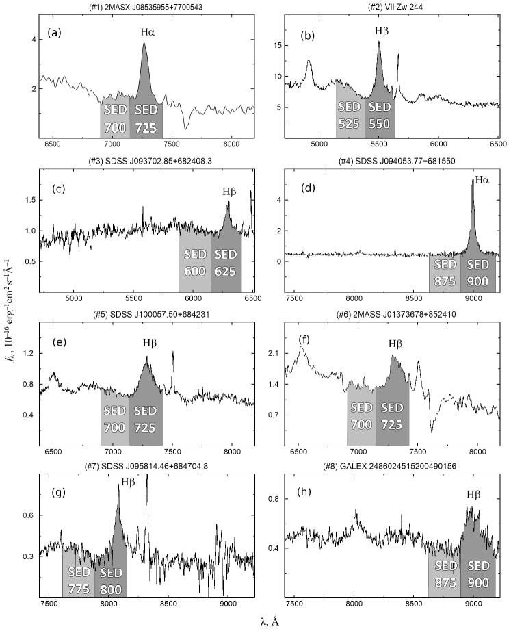
Figure 1: SED bands overplotted on the spectra of the studied AGN.

From the known relations $R_{\rm BLR}-L$ for the H_β line the expected delays $\tau$ were calculated for the sample (see Table. 1). For objects with redshifts up to 0.5—##1,3–5—the flux $L_{\lambda}$ at 5100 Å measured in the range 4400–5850 Å was calculated. Then from the relation $R_{\rm BLR}-L_{\lambda}$ (5100 Å), where $R_{\rm BLR}$ is the size of the BLR region in the line H_β RL5100 :

$$\log(R_{\rm BLR})=-21.3^{+2.9}_{-2.8}+0.519^{+0.063}_{-0.066}\log(\lambda L_{\lambda}),$$

where $L_{\lambda}=L_{\lambda}$ (5100 Å) is a flux at 5100 Å.

In the case of $z>0.5$, as well as for the object #2, which spectral data are available only in a small wavelength range (3500–7000Å), the $L_{\lambda}$ (5100 Å) range goes beyond the available optical spectra. In this regard, for objects ##2,6–8 the calibration in the line $L_{\lambda}(\text{H}_{\beta})$ Greene10 was used:

$$\log(R_{10})=0.85\pm 0.05+(0.53\pm 0.04)\log(L_{43}(\text{H}_{\beta})),$$

where $R_{10}=R_{\rm BLR}/10$ lt days is the size of the BLR region, normalized to the 10 lt days,$L_{43}(\text{H}_{\beta})=L_{\lambda}(\text{H}_{\beta})/10^{43}$ erg s^-1 is the luminosity in the H_β line normalized to $10^{43}$ erg s^-1. In Table 1 the expected delays $\tau$ are given with an accuracy of 10%.

It is known that the matter in BLR is stratified Peterson94 ; Baldwin , and the region emitting in H_α is bigger than the region emitting in H_β. However, the calibration relation $L_{\lambda}(\text{H}_{\alpha})$ is unpopular since for many AGN the narrow line N II (6583 Å) belonging to the emission of narrow-line region clouds (NLR) makes a large contribution to the H_α flux. To estimate the possible difference for the delay of variation in H_α for objects #1 and #4, we used the catalog data BentzKatz15 for 29 AGN for delays known in both H_α and H_β lines. Also, we used data on Sy 1 3C 390.3 obtained from spectropolarimetric monitoring on the 6-m BTA telescope Af15 . A comparison of the observed lag in the lines is shown in Fig. 2. The slope of the line is equal to $k=\tau({\rm H}\beta)/\tau({\rm H}\alpha)=0.88\pm 0.03$. Thus, the H_α lag for #1 and #4 coincides with the expected by H_β within 10%.

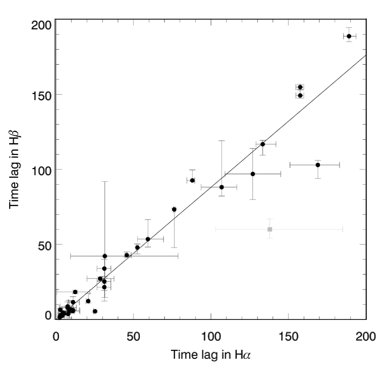
Figure 2: Comparison of the observed time lag in H_β line relative to the time lag in H_α line according to the catalog BentzKatz15 (black) and the monitoring Af15 (gray).

III Observations

III.1 Instruments

Since February 2018, observations of the AGN sample have been carried out monthly on grey and bright nights at Zeiss-1000 telescope of the SAO RAS using MaNGaL (MApper of Narrow GAlaxy Lines Pulkovo ) and MMPP (Multi-Mode Photometer-Polarimeter) mmpp devices in photometric mode with 10 medium-band interference SED filters. The size of the field of view was 8.${}^{\prime}7\times 8.^{\prime}7$ for MaNGaL and 7.${}^{\prime}2\times 7.^{\prime}$2 for MMPP.

Three different detectors were used during the observations: Andor CCD iKon-M 934 (1024$\times$1024 px), Andor Neo sCMOS (2560$\times$2160 px), and Raptor Photonics Eagle V CCD (2048$\times$2048 px). The quantum efficiency of these detectors in the needed bands is shown in Table 2. Water cooling was used for all three cases to minimize noise.

Table 2: Quantum efficiency of detectors in the studied photometric bands

Detector	Quantum efficiency, %
	5500 Å	6000 Å	7000 Å	8000 Å	9000 Å
Andor iKon-M 934	95	96	91	77	47
Andor Neo sCMOS	54	56	49	31	14
Eagle V CCD	92	95	89	75	50

III.2 Photometric Standards

Observations of the sample were alternated with observations of spectrophotometric standard stars from the paper Oke90 . The standards were observed before and/or after obtaining a frame with the object field in the same filter and as close as possible to the zenith distance. This method of observations makes it possible to determine the relation between the instrumental units and the absolute ones beyond the atmosphere and, consequently, to bind the flux of the selected stars in the field of the object to the absolute magnitudes to create a network of the local standards.

We have used a system of AB-magnitudes. This system is defined so that for a monochromatic flux $f_{\nu}$ measured in erg s^-1 cm^-2 Hz^-1:

$$m_{AB}=-2.5\cdot\log(f_{\nu})-48.60.$$

Since the transmittance of SED filters is measured in laboratory, we denote it as a function $filter(\nu)$ and convolute with a spectral energy distribution of the photometric standard $f_{\nu}$ to determine its extra-atmospheric AB-value according to the formula:

$$m_{AB}=-2.5\cdot\log\Bigg{[}\frac{\int f_{\nu}\cdot filter(\nu)\cdot d\nu}{\int filter(\nu)\cdot d\nu}\Bigg{]}-48.60,$$

where the flux of the standard is $f_{\nu}$ also in erg s^-1 cm^-2 Hz^-1.

In Table 3 the calculated AB-magnitudes of the observed standards for the used SED filters are given.

Table 3: The photometric fluxes of the standard stars in AB-magnitudes in the SED bands

Stars-	$m_{\rm AB}$, mag
standards	SED 525	SED 550	SED 600	SED 625	SED 700	SED 725	SED 775	SED 800	SED 875	SED 900
G $193-74$	15.63	15.61	15.58	15.58	15.58	15.59	15.61	15.62	15.68	15.73
BD $+75\hbox{${}^{\circ}$}325$	9.47	9.56	9.73	9.81	10.03	10.10	10.22	10.28	10.46	10.51
Feige 34	11.09	11.17	11.35	11.43	11.63	11.69	11.79	11.84	11.90	12.05
BD $+33\hbox{${}^{\circ}$}2642$	10.71	10.78	10.91	10.97	11.13	11.18	11.28	11.33	11.43	11.45
BD $+28\hbox{${}^{\circ}$}4211$	10.43	10.52	10.70	10.78	10.99	11.05	11.18	11.24	11.42	11.50
BD $+25\hbox{${}^{\circ}$}4655$	9.60	9.69	9.87	9.95	10.16	10.22	10.35	10.41	10.59	10.68
Feige 110	11.76	11.85	12.03	12.10	12.32	12.39	12.50	12.57	12.74	12.79

For the observational data reduction and subsequent measurements, the IDL software was used. During each observational night, we received calibration images (flat frames for each filter at the twilight sky moving the telescope , bias/dark) to correct data for additive and multiplicative errors. Photometric standards were also observed at different zenithal distances to control the extinction coefficient within the night. To account the light absorption in the atmosphere, the air masses were calculated according to Hardie :

$$\begin{array}[]{rcl}M=&\sec(z)&\!\!-0.0018167[\sec(z)-1]\\[-5.0pt] &&\!\!-0.002875[\sec(z)-1]^{2}\\[-5.0pt] &&\!\!-0.0008083[\sec(z)-1]^{3}.\end{array}$$

The method of aperture photometry was used to determine the flux of objects. Therefore, to correctly account the sky background, the traces of cosmic rays fell close to the object were removed from images.

There is a misconception that shooting a sufficiently large number of frames and summing them it is possible to improve the signal/noise ratio S/N. The criteria for the correct evaluation of the S/N ratio are given in the paper Afanasieva2016 . Since the image processing has to work with random flux values it is necessary to correctly determine the estimates. So, each frame is processed independently, and statistical evaluation is made by averaging the random value by robust methods giving its unbiased estimate.

IV RESULTS

IV.1 Local Standards

To measure the absolute AGN variability we have selected the candidates for local standard stars in the fields of each object. Over a long period, their brightness must remain constant, plus it should be comparable to the AGN magnitude to avoid overexposure of the signal and hence the effects of deviation from linearity on the detector at long exposures. The use of local comparison stars for differential photometry significantly increases the accuracy of measurements of the studied AGN flux, and also allows one to observe at grey and bright nights and under unstable atmospheric transparency.

As a result of the first year of monitoring, a network of comparison stars was formed for photometric binding of AGN under unstable atmosphere to obtain calibrated light curves in emission line and continuum. Photometric errors on average do not exceed $\sigma$ = 0.02 mag.

Table 4: Comparison stars for the sample objects: (1) coordinates for the J2000 epoch; (2) AB-magnitudes of the comparison star in the filter corresponding to the observed range of the object continuum; (3) AB-magnitudes of the comparison star in the filter corresponding to the broad emission line of the object

	RA Dec (J2000)	Continuum	Line		RA Dec (J2000)	Continuum	Line
(#)	(1)	(2)	(3)	(#)	(1)	(2)	(3)
#1		SED700	SED725	#5		SED700	SED725
1-1	08h54m16$\,.\!\!^{\rm s}$3 $+76\hbox{${}^{\circ}$}59\hbox{${}^{\prime}$}44\hbox{${}^{\prime\prime}$}$	15.00 $\pm$ 0.01	14.95 $\pm$ 0.01	5-1	10h00m55$\,.\!\!^{\rm s}$4 $+68\hbox{${}^{\circ}$}41\hbox{${}^{\prime}$}01\hbox{${}^{\prime\prime}$}$	16.26 $\pm$ 0.01	16.23 $\pm$ 0.01
1-2	08h53m48$\,.\!\!^{\rm s}$5 $+76\hbox{${}^{\circ}$}59\hbox{${}^{\prime}$}27\hbox{${}^{\prime\prime}$}$	15.16 $\pm$ 0.01	15.13 $\pm$ 0.01	5-2	10h00m50$\,.\!\!^{\rm s}$0 $+68\hbox{${}^{\circ}$}40\hbox{${}^{\prime}$}32\hbox{${}^{\prime\prime}$}$	15.70 $\pm$ 0.01	15.70 $\pm$ 0.01
#2		SED525	SED550	#6		SED700	SED725
2-1	08h44m32$\,.\!\!^{\rm s}$0 $+76\hbox{${}^{\circ}$}53\hbox{${}^{\prime}$}49\hbox{${}^{\prime\prime}$}$	12.54 $\pm$ 0.01	12.47 $\pm$ 0.01	6-1	01h37m15$\,.\!\!^{\rm s}$5 $+85\hbox{${}^{\circ}$}22\hbox{${}^{\prime}$}28\hbox{${}^{\prime\prime}$}$	14.82 $\pm$ 0.01	14.84 $\pm$ 0.01
2-2	08h45m22$\,.\!\!^{\rm s}$4 $+76\hbox{${}^{\circ}$}50\hbox{${}^{\prime}$}12\hbox{${}^{\prime\prime}$}$	14.03 $\pm$ 0.01	13.96 $\pm$ 0.01	6-2	01h36m44$\,.\!\!^{\rm s}$1 $+85\hbox{${}^{\circ}$}23\hbox{${}^{\prime}$}31\hbox{${}^{\prime\prime}$}$	15.40 $\pm$ 0.01	15.43 $\pm$ 0.01
#3		SED600	SED625	#7		SED775	SED800
3-1	09h36m44$\,.\!\!^{\rm s}$7 $+68\hbox{${}^{\circ}$}25\hbox{${}^{\prime}$}46\hbox{${}^{\prime\prime}$}$	13.73 $\pm$ 0.01	13.72 $\pm$ 0.01	7-1	09h58m21$\,.\!\!^{\rm s}$7 $+68\hbox{${}^{\circ}$}45\hbox{${}^{\prime}$}58\hbox{${}^{\prime\prime}$}$	15.48 $\pm$ 0.01	15.45 $\pm$ 0.01
3-2	09h36m54$\,.\!\!^{\rm s}$6 $+68\hbox{${}^{\circ}$}24\hbox{${}^{\prime}$}39\hbox{${}^{\prime\prime}$}$	16.63 $\pm$ 0.07	16.60 $\pm$ 0.06	7-2	09h58m45$\,.\!\!^{\rm s}$4 $+68\hbox{${}^{\circ}$}45\hbox{${}^{\prime}$}09\hbox{${}^{\prime\prime}$}$	16.93 $\pm$ 0.01	16.84 $\pm$ 0.01
#4		SED875	SED900	#8		SED875	SED900
4-1	09h40m51$\,.\!\!^{\rm s}$8 $+68\hbox{${}^{\circ}$}15\hbox{${}^{\prime}$}10\hbox{${}^{\prime\prime}$}$	15.57 $\pm$ 0.02	15.54 $\pm$ 0.02	8-1	10h01m56$\,.\!\!^{\rm s}$4 $+69\hbox{${}^{\circ}$}32\hbox{${}^{\prime}$}46\hbox{${}^{\prime\prime}$}$	16.13 $\pm$ 0.02	16.16 $\pm$ 0.03
4-2	09h41m06$\,.\!\!^{\rm s}$9 $+68\hbox{${}^{\circ}$}16\hbox{${}^{\prime}$}41\hbox{${}^{\prime\prime}$}$	14.99 $\pm$ 0.02	14.95 $\pm$ 0.02	8-2	10h02m04$\,.\!\!^{\rm s}$6 $+69\hbox{${}^{\circ}$}34\hbox{${}^{\prime}$}02\hbox{${}^{\prime\prime}$}$	17.26 $\pm$ 0.02	17.19 $\pm$ 0.04

The results obtained for all comparison stars are summarized in Table 4.

IV.2 Preliminary Result

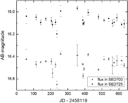
Figure 3: The light curves of AGN #1, obtained in the SED filters corresponding to the flux in the line and in the continuum near. The Julian dates starts on January 1, 2018.

The measurements of the studied AGN fluxes were carried out relative to the most stable reference stars assumed to be the local standards. The light curves in the continuum and the line of one of the most frequently observed AGN #1 (2MASX J08535955+7700543) are shown in Fig. 3.

After subtracting the continuum flux from the total flux in the line, there is a short-term variability at the level of 0.2 AB-magnitudes of the both fluxes, and the character of the variability is repeated. The observed amplitude exceeds the average error of AGN radiation measurement: the differential photometry method provides an accuracy of $\sim$0.03 mag.

To estimate the time delay between the two light curves of the object #1 of the sample, the classical cross-correlation method ICCF was used as well as the method using the code JAVELIN Zu16 ; jav . The results are presented in Fig. 4.

IV.2.1 Classical Cross-Correlation Method

The solid curve in Fig. 4 denotes the interpolated cross-correlation function (ICCF). Fitting the Gaussian to the most powerful ICCF peak gives us an estimate of the time delay $\tau(ICCF)=32.2\pm 10.6$ days. In this estimate, we use the half-width of the Gaussian interpolation as the measurement error. Note that to obtain a contrast peak, it is also necessary to subtract the contribution of the continuum to the total flux in the emission line.

IV.2.2 JAVELIN

Fig. 4 shows the JAVELIN method as a histogram obtained using JAVELIN (Just Another Vehicle for Estimating Lags in Nuclei) code implemented in the python programming language. We describe briefly the content of the procedure for determining $\tau$ using this method. The first step is to build a continuum model using the DRW (dumped random walk) method. As a result, we have posterior distributions of two DRW parameters of continuum variability—amplitude and time scale calculated on the basis of MCMC sampling (Markov chain Monte Carlo). The second step is to interpolate the light curve of the continuum based on the parameters defined in the first step and then offset, smooth, and scale it to compare with the observed line light curve. After another run of the MCMC algorithm, the JAVELIN package determines the desired posterior time delay distribution between the light curves. As a result, we got the value $\tau({\rm JAVELIN})=39.5_{-15.8}^{+23.0}$ days. The estimate itself corresponds to the median value of the most powerful peak, located in the range from $-20$ to 80 days in Fig. 4. The lower and upper estimates of the time delay correspond to the limits of the highest density interval of the posterior distribution, which are calculated using JAVELIN.

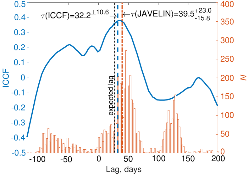
Figure 4: Cross-correlation analysis of the time delay between the continuum flux and the flux in the emission line for 2MASS J08535955+7700543 (#1) using two methods: classical ICCF (solid interpolated curve) and JAVELIN (histogram obtained using JAVELIN). Corresponding time delay estimates marked by dashed ($\tau(ICCF)$) and dash-dotted ($\tau({\rm JAVELIN})$) vertical lines. The dotted line shows the expected value of $\tau$ from calibrations.

IV.2.3 General Comment

So, to illustrate the technique efficiency, we used AGN #1 light curves and revealed estimates of the time delay $\tau(ICCF)=32.2^{\pm 10.6}$ days and $\tau({\rm JAVELIN})=39.5_{-15.8}^{+23.0}$ days. Within the limits of accuracy, our estimates are in good agreement with each other and with the expected time delay $\tau\approx 27$ days from the calibration relations. Despite the fact that cross-correlation peaks are confidently detected, we assume a continuation of the accumulation of observational data for the light curves to refine the result of AGN #1 cross-correlation analysis. A direct comparison of the time delay error values $\Delta\tau$ for ICCF and JAVELIN methods is inappropriate and requires additional research within this project. Both methods work well even in the presence of systematic errors Yu19 .

It should be noted that the measurement error of the delay $\Delta\tau$ is closely connected with the sampling period of the light curves $t_{cad}$, i.e., the time between sets of observations Zu16 . Over the past year, the average period of $t_{cad}$ was $\sim$20-25 days. To specify the value of the delay $\tau$ it is necessary to increase the number of sets of observations, thereby reducing the sampling, which is especially important for active nuclei with the expected delay of the radiation with the lags of the order of several tens of days, for example, #1 and #2.

V Conclusions

Within this work, the following results were obtained.

• 1. The observations by the photometric reverberation mapping method are adapted for telescopes of 1-meter class and are independent of the device used.

• 2. For each of the studied active nuclei in the range of redshifts $0.1<z<0.8$, a network of secondary standards was determined, which allows further use of the differential photometry method. The photometric accuracy is on average 0.03 mag, which is an order of magnitude greater than the expected amplitude of the AGN variability.

• 3. Preliminary results of the object 2MASX J08535955+7700543 (#1) reverberation mapping are shown in Fig. 3. It is seen that the observed object is variable, and the used method is stable. Applying the classical cross-correlation function and JAVELIN gave estimates of the time delay $\tau(ICCF)=32.2^{\pm 10.6}$ days and$\tau({\rm JAVELIN})=39.5_{-15.8}^{+23.0}$ days that are consistent with each other and within the accuracy of the existing calibration relations.

VI Acknowledgments

The authors are sincerely grateful to the reviewer for fruitful comments, which contributed to the improvement to the article.

The authors thank V. L. Afanasiev for useful discussions and comments.

FUNDING

The work is executed at support of RFBR grant 18-32-00826. Observations on the telescopes of SAO RAS are carried out with the support of the Ministry of science of the Russian Federation.

CONFLICT OF INTERESTS

The authors declare no conflict of interest regarding this paper.

References

- (1) R. D. Blandford and C. F. McKee, Astrophys. J. 255, 419 (1982).
- (2) B. M. Peterson, Publ. Astron. Soc. Pacific 105, 247 (1993).
- (3) A. M. Cherepashchuk and V. M. Lyutyi, Astrophys. Letters13, 165 (1973).
- (4) I. I. Antokhin and N. G. Bochkarev, Sov. Astron. 27, 261 (1983).
- (5) C. M. Gaskell and L. S. Sparke, Astrophys. J. 305, 175 (1986).
- (6) B. M. Peterson, L. Ferrarese, K. M. Gilbert, et al., Astrophys. J. 613, 682 (2004).
- (7) M. C. Bentz and S. Katz, Publ. Astron. Soc. Pacific 127, 67 (2015).
- (8) P. Du, K.-X. Lu, Z.-X. Zhang, et al., Astrophys. J. 825, 126 (2016).
- (9) L. Jiang, Y. Shen, I. D. McGreer, et al., Astrophys. J. 818, 137 (2016).
- (10) F. Pozo Nuñez, D. Chelouche, S. Kaspi, and S. Niv, Publ. Astron. Soc. Pacific 129, 094101 (2017).
- (11) Y. Shen, W. N. Brandt, K. S. Dawson, et al., Astrophys. J. Suppl. 216, 4 (2015).
- (12) C. J. Grier, J. R. Trump, Y. Shen, et al., Astrophys. J. 851, 21 (2017).
- (13) C. J. Grier, J. R. Trump, Y. Shen, et al., Astrophys. J. 868, 76 (2018).
- (14) B. Czerny, A. Olejak, M. Ralowski, et al., arXiv e-prints arXiv:1901.09757 (2019).
- (15) S. Kaspi, D. Maoz, H. Netzer, et al., Astrophys. J. 629, 61 (2005).
- (16) M. C. Bentz, J. L. Walsh, A. J. Barth, et al., Astrophys. J. 705, 199 (2009).
- (17) M. Haas, R. Chini, M. Ramolla, et al., Astron. and Astrophys. 535, A73 (2011).
- (18) B. Abolfathi, D. S. Aguado, G. Aguilar, et al., Astrophys. J. Suppl. 235, 42 (2018).
- (19) T. A. Boroson and R. F. Green, Astrophys. J. Suppl. 80, 109 (1992).
- (20) J. Y. Wei, D. W. Xu, X. Y. Dong, and J. Y. Hu, Astron. and Astrophys. Suppl. 139, 575 (1999).
- (21) M. C. Bentz, B. M. Peterson, H. Netzer, et al., Astrophys. J. 697, 160 (2009).
- (22) J. E. Greene, C. E. Hood, A. J. Barth, et al., Astrophys. J. 723, 409 (2010).
- (23) B. M. Peterson, in Reverberation Mapping of the Broad-Line Region in Active Galactic Nuclei, Edited by P. M. Gondhalekar, K. Horne, and B. M. Peterson (1994), Astronomical Society of the Pacific Conference Series, vol. 69, p. 1.
- (24) J. A. Baldwin, G. J. Ferland, K. T. Korista, et al., Astrophys. J. 582, 590 (2003).
- (25) V. L. Afanasiev, A. I. Shapovalova, L. Č. Popović, and N. V. Borisov, Monthly Notices Royal Astron. Soc. 448, 2879 (2015).
- (26) A. E. Perepelitsyn, A. V. Moiseev, and D. V. Oparin, “”MaNGaL focal reducer with tunable interference filter for small and medium telescopes (in Russian)”,” Proceedings of the VII Pulkovo youth astronomical conference (Pulkovo, St. Petersburg, 28-31 may 2018), Izvestia GAO, 226, pp. 65-70.
- (27) J. B. Oke, Astron. J. 99, 1621 (1990).
- (28) W. A. Hiltner, Astronomical techniques. (1962).
- (29) I. V. Afanasieva, Astrophysical Bulletin 71, 366 (2016).
- (30) Y. Zu, C. S. Kochanek, S. Kozłowski, and B. M. Peterson, Astrophys. J. 819, 122 (2016).
- (31) D. Mudd, P. Martini, Y. Zu, et al., Astrophys. J. 862, 123 (2018).
- (32) Z. Yu, C. S. Kochanek, B. M. Peterson, et al., arXiv e-prints arXiv:1909.03072 (2019).