Lattice QCD calculation of the pion charge radius using a model-independent method

Abstract

We use a method to calculate the hadron’s charge radius without model-dependent momentum extrapolations. The method does not require the additional quark propagator inversions on the twisted boundary conditions or the computation of the momentum derivatives of quark propagators and thus is easy to implement. We apply this method to the calculation of pion charge radius $\langle r_{\pi}^{2}\rangle$. For comparison, we also determine $\langle r_{\pi}^{2}\rangle$ with the traditional approach of computing the slope of the form factors. The new method produces results consistent with those from the traditional method and with statistical errors 1.5 - 1.9 times smaller. For the four gauge ensembles at the physical pion masses, the statistical errors of $\langle r_{\pi}^{2}\rangle$ range from 2.1% to 4.6% by using $\lesssim 50$ configurations. For the ensemble at $m_{\pi}\approx 340$ MeV, the statistical uncertainty is even reduced to a sub-percent level.

Introduction. – In particle physics, hadron is a bound state of quarks and gluons, which are held together by the strong interaction force. Different from a point-like particle, hadron has a rich internal structure. One intrinsic property of a hadron is its charge radius, which corresponds to the spatial extent of the distribution of the hadron’s charge. The accurate determination of the charge radius not only leaves us useful information on the size and the structure of the hadron, but also provides crucial precision tests of the Standard Model at low energy. It is of special importance in resolving the proton radius puzzle Pohl et al. (2010), where two recent experiments report results which agree with the previous ones obtained by spectroscopy of muonic hydrogen Bezginov et al. (2019); Xiong et al. (2019) and represent a decisive step towards solving the puzzle for a decade.

In the theoretical study, the charge radius of the hadron is essentially a non-perturbative quantity. It is highly appealing to have a reliable calculation of this quantity with robust uncertainty estimate using lattice QCD. The traditional approach for determining the charge radius on the lattice involves the extrapolation of the expression $(F(q^{2})-1)/q^{2}$ to zero momentum transfer $q^{2}=0$, where $F(q^{2})$ is the vector form factor. The choices of the fit ansatz and fitting window would inevitably bring systematic uncertainties from modeling the momentum dependence of $F(q^{2})$. To reduce such uncertainties, twisted boundary conditions Bedaque (2004); de Divitiis et al. (2004) and momentum derivatives of quark propagators de Divitiis et al. (2012); Hasan et al. (2018) are proposed and used.

In this work, we use an approach to directly determine the charge radius without the momentum extrapolations. The method is easy to implement on the lattice calculation with no requirement on twisted boundary conditions or sequential-source propagators containing momentum derivatives. As an example, we apply the method to the calculation of pion’s charge radius. This quantity has been determined by various groups using the traditional method Brömmel et al. (2007); Aoki et al. (2009); Wang et al. (2018), twisted boundary conditions Frezzotti et al. (2009); Boyle et al. (2008); Nguyen et al. (2011); Brandt et al. (2013); Aoki et al. (2016); Koponen et al. (2016); Alexandrou et al. (2018) as well as the momentum extrapolations from the timelike region Meyer (2011); Feng et al. (2015); Erben et al. (2019). In our study we find that the statistical errors can be reduced to 2.1% - 4.6% at the physical point. At $m_{\pi}\approx 340$ MeV, we obtain a sub-percent statistical uncertainty 0.8%, which is about 6 - 13 times smaller than that from the previous calculations at the similar pion masses Frezzotti et al. (2009); Boyle et al. (2008); Aoki et al. (2009); Nguyen et al. (2011); Brandt et al. (2013); Aoki et al. (2016).

Upon finishing this work, we note that a similar idea has been proposed by C. C. Chang et. al. in Ref. Bouchard et al. (2016) to calculate the proton charge radius. The earlier work along this direction can be traced back to mid 90’s to calculate the slope of the Isgur-Wise function at zero-recoil Aglietti et al. (1994); Lellouch et al. (1995). When utilizing this method, we find that it cannot be used directly in the calculation of the pion charge radius as it suffers from significant finite-volume effects. We therefore develop the techniques to solve the problems, which are described in the following context.

Charge radius in the continuum theory. – We start with a Euclidean hadronic function in the infinite volume

$$H_{\phi}(x)=H_{\phi}(t,\vec{x})=\langle 0|\phi(t,\vec{x})J_{\mu}(0)|\pi(\vec{0})\rangle,$$ (1)

where $|\pi(\vec{0})\rangle$ is a pion initial state carrying zero spatial momentum. $J_{\mu}$ is an electromagnetic vector current. $\phi$ is an interpolating operator, which can annihilate a pion state. It can be chosen as e.g. a pseduoscalar operator $\bar{u}\gamma_{5}d$ or an axial vector current $\bar{u}\gamma_{\mu}\gamma_{5}d$. In this study we use the hadronic function $H(x)=\langle 0|A_{4}(x)J_{4}(0)|\pi(\vec{0})\rangle$ with $\phi=A_{4}=\bar{u}\gamma_{4}\gamma_{5}d$.

At large time $t$, $H(x)$ is saturated by the single pion state

$$H(x)\doteq H_{\pi}(x)\equiv\int\frac{d^{3}\vec{p}}{(2\pi)^{3}}\frac{f_{\pi}}{2}(E+m_{\pi})F_{\pi}(q^{2})e^{-Et-i\vec{p}\cdot\vec{x}},$$ (2)

where the symbol $\doteq$ denotes the omission of the excited states. The decay constant $f_{\pi}\approx 130\leavevmode\nobreak\ \mathrm{MeV}$ is from PCAC relation $\langle 0|A_{4}(0)|\pi(\vec{p})\rangle=Ef_{\pi}$ and $E=\sqrt{m_{\pi}^{2}+\vec{p}^{2}}$ the pion’s energy. The pion form factor $F_{\pi}(q^{2})$ can be extracted from the matrix element $\langle\pi(\vec{p})|J_{4}(0)|\pi(\vec{0})\rangle=(E+m_{\pi})F_{\pi}(q^{2})$, with $q^{2}=(E-m_{\pi})^{2}-\vec{p}^{2}$. In the Taylor expansion

$$F_{\pi}(q^{2})=\sum_{n=0}^{\infty}c_{n}\left(\frac{q^{2}}{m_{\pi}^{2}}\right)^{n},$$ (3)

$c_{0}=1$ is required by the charge conservation and $c_{1}$ is related to the mean-square charge radius via $c_{1}=\frac{m_{\pi}^{2}}{6}\langle r_{\pi}^{2}\rangle$.

The spatial Fourier transform of Eq. (2) yields

$$\tilde{H}(t,\vec{p})\doteq\tilde{H}_{\pi}(t,\vec{p})\equiv\frac{f_{\pi}}{2}(E+m_{\pi})F_{\pi}(q^{2})e^{-Et}.$$ (4)

The derivative of $\tilde{H}(t,\vec{p})$ at $|\vec{p}|^{2}=0$ leads to

$$D(t)\equiv m_{\pi}^{2}\frac{\partial\tilde{H}(t,\vec{p})}{\partial|\vec{p}|^{2}}\bigg{|}_{|\vec{p}|^{2}=0}=-\frac{m_{\pi}^{2}}{3!}\int d^{3}\vec{x}\,|\vec{x}|^{2}H(x),$$ (5)

while for $\tilde{H}_{\pi}(t,\vec{p})$ we have

$$\frac{m_{\pi}^{2}}{\tilde{H}_{\pi}(t,\vec{0})}\frac{\partial\tilde{H}_{\pi}(t,\vec{p})}{\partial|\vec{p}|^{2}}\bigg{|}_{|\vec{p}|^{2}=0}=\frac{1}{4}-\frac{m_{\pi}t}{2}-c_{1},$$ (6)

with $\tilde{H}_{\pi}(t,\vec{0})=f_{\pi}m_{\pi}e^{-m_{\pi}t}$. Combining Eq. (5) and (6), one can determine $c_{1}$ using $H(x)$ as input through

$$R(t)=\frac{D(t)}{\tilde{H}(t,\vec{0})}\doteq\frac{1}{4}-\frac{m_{\pi}t}{2}-c_{1}.$$ (7)

Charge radius on the lattice. – In a realistic lattice QCD calculation with a lattice size of $\sim 5$ fm, the finite volume truncation effects are very large as at the edge of box the integrand in Eq. (5) scales as $m_{\pi}^{2}|\vec{x}|^{2}\exp(-m_{\pi}\sqrt{\vec{x}^{2}+t^{2}})\sim 0.53$ with $\sqrt{\vec{x}^{2}+t^{2}}\approx|\vec{x}|\sim 2.5$ fm. Therefore Eqs. (5) - (7) are too sloppy to be used in a precision calculation. On the lattice with a size $L$ and a lattice spacing $a$, the hadronic function $H^{(L)}(x)$ is approximated by

$$H^{(L)}(x)\doteq H_{\pi}^{(L)}(x)\equiv\frac{1}{L^{3}}\sum_{\vec{p}\in\Gamma}\tilde{H}_{\pi}(t,\vec{p})\cos(\vec{p}\cdot\vec{x}),$$ (8)

where $\Gamma$ indicates a set of discrete momenta $\vec{p}=\frac{2\pi}{L}\vec{n}$ ($\vec{n}\in\mathbb{Z}^{3}$) with component $p_{i}$ ranging from $-\frac{\pi}{a}\leq p_{i}<\frac{\pi}{a}$. Similar to Eq. (5), we define

$$D^{(L)}(t)\equiv-\frac{m_{\pi}^{2}}{3!}\sum_{\vec{x}\in\mathbb{L}^{3}}|\vec{x}|^{2}H^{(L)}(x),$$ (9)

with $\vec{x}\in\mathbb{L}^{3}$ running through $x_{i}=-L/2,-L/2+a,\cdots,L/2-a$ for $i=1,2,3$.

Considering the lattice discretization, we propose to use the lattice dispersion relation $\hat{E}^{2}=\hat{m}^{2}+\sum_{i}\hat{p}_{i}^{2}$ with $a\hat{E}=2\sinh(aE/2)$, $a\hat{m}=2\sinh(am_{\pi}/2)$ and $a\hat{p}_{i}=2\sin(ap_{i}/2)$. The notation $\sum_{i}$ indicates the summation over all spatial directions. We further adopt the lattice-modified relations

$$\langle 0|A_{4}(0)|\pi(\vec{p})\rangle=\hat{E}f_{\pi},$$

$$\langle\pi(\vec{p})|J_{4}(0)|\pi(\vec{0})\rangle=(\hat{E}+\hat{m})F_{\pi}(\hat{q}^{2}),$$

$$\frac{1}{\hat{p}_{0}^{2}-\hat{E}^{2}}\bigg{|}_{p_{0}\to E}=\frac{1}{2\tilde{E}}\frac{1}{p_{0}-E}$$ (10)

with $a\hat{p}_{0}=2\sinh(ap_{0}/2)$ and $a\tilde{E}=\sinh(aE)$. The square of momentum transfer $\hat{q}^{2}$ is given by $\hat{q}^{2}=(\hat{E}-\hat{m})^{2}-\sum_{i}\hat{p}_{i}^{2}$.

As a next step, we construct a ratio

$$R^{(L)}(t)=\frac{D^{(L)}(t)}{\tilde{H}^{(L)}(t,\vec{0})},$$ (11)

where $\tilde{H}^{(L)}(t,\vec{0})$ is defined as

$$\tilde{H}^{(L)}(t,\vec{0})\equiv\sum_{\vec{x}\in\mathbb{L}^{3}}H^{(L)}(x)\doteq\sum_{\vec{x}\in\mathbb{L}^{3}}H_{\pi}^{(L)}(x)=\tilde{H}_{\pi}(t,\vec{0}).$$ (12)

Note that $R^{(L)}(t)$ can be written as

$$R^{(L)}(t)\doteq\sum_{n=0}^{\infty}\beta_{n}^{(L)}(t)\,c_{n}$$ (13)

with the coefficients $\beta_{n}^{(L)}(t)$ known explicitly through

$$\beta_{n}^{(L)}(t)=-\frac{m_{\pi}^{2}}{3!}\sum_{\vec{x}\in\mathbb{L}^{3}}|\vec{x}|^{2}I_{n}(x)$$

$$I_{n}(x)=\frac{1}{L^{3}}\sum_{\vec{p}\in\Gamma}\frac{\hat{E}}{\tilde{E}}\frac{\tilde{m}}{\hat{m}}\frac{\hat{E}+\hat{m}}{2\hat{m}}\left(\frac{\hat{q}^{2}}{m_{\pi}^{2}}\right)^{n}e^{-(E-m_{\pi})t}\cos(\vec{p}\cdot\vec{x}).$$

Here we have used the relations in Eq. (Lattice QCD calculation of the pion charge radius using a model-independent method). The value of $c_{1}$ can be approximated by $\left(R^{(L)}(t)-\beta_{0}^{(L)}(t)\right)/\beta_{1}^{(L)}(t)$. In Eq. (Lattice QCD calculation of the pion charge radius using a model-independent method) the lattice cutoff effects from large $\hat{q}^{2}$ are safely controlled by the suppression of $e^{-(E-m_{\pi})t}$ at sufficiently large $t$. Thus the continuum limit ($a\to 0$) can be taken safely. But one shall not consider to take the extreme limit of $t\to\infty$. In that limit, the hadronic function is dominated by the pion state with zero momentum, while the charge radius, as a slope of the form factor, requires the information from different momenta. Taking very large $t$ certainly makes the analysis less interesting. Luckily, $t$ is only required to suppress the excited-state effects and is not necessary to be very large.

Note that when $a\to 0$ and $L\to\infty$, all the coefficients $\beta_{n}^{(L)}$ for $n\geq 2$ vanish as in Eq. (7). We can consider the contamination from $c_{n\geq 2}$ terms as the systematic effects, which are well under control by using the fine lattice spacings and large volumes. Therefore Eq. (13) provides a direct way to calculate the pion charge radius using the lattice quantity $H^{(L)}(x)$ as input.

Error reduction. – The hadronic function $H^{(L)}(x)$ is exponentially suppressed at large $|\vec{x}|$ and thus the lattice data near the boundary of the box mainly contribute to the noise rather than the signal. To reduce the statistical error, we introduce an integral range $\xi L$ with $\xi\leq\frac{\sqrt{3}}{2}$ (For $\xi\leq\frac{1}{2}$ the range has a spherical shape.) and define

$$D_{k}^{(L,\xi)}(t)\equiv(-1)^{k}\frac{m_{\pi}^{2k}}{(2k+1)!}\sum_{|\vec{x}|\leq\xi L}|\vec{x}|^{2k}H^{(L)}(x),$$ (15)

which are related to $c_{n}$ through

$$\frac{D_{k}^{(L,\xi)}(t)}{\tilde{H}^{(L)}(t,\vec{0})}\doteq\sum_{n=0}^{\infty}\beta_{k,n}^{(L,\xi)}(t)\,c_{n}$$ (16)

with

$$\beta_{k,n}^{(L,\xi)}(t)=(-1)^{k}\frac{m_{\pi}^{2k}}{(2k+1)!}\sum_{|\vec{x}|\leq\xi L}|\vec{x}|^{2k}I_{n}(x).$$ (17)

To remove the systematic contamination from the $c_{2}$ term, we use both $D_{1}^{(L,\xi)}(t)$ and $D_{2}^{(L,\xi)}(t)$ to construct the ratio $R^{(L,\xi)}(t)$

$$R^{(L,\xi)}(t)=\frac{f_{1}D_{1}^{(L,\xi)}(t)+f_{2}D_{2}^{(L,\xi)}(t)}{\tilde{H}^{(L)}(t,\vec{0})}+h,$$ (18)

where the parameters $f_{1}$, $f_{2}$ and $h$ are chosen to remove the $c_{0}$ and $c_{2}$ terms. Namely, we impose three conditions

$$\sum_{k=1,2}f_{k}\beta_{k,n}^{(L,\xi)}(t)=b_{n},\quad\text{with }b_{0}=-h,\,b_{1}=1,\,b_{2}=0.$$ (19)

Under these conditions $R^{(L,\xi)}(t)$ is given by

$$R^{(L,\xi)}(t)\doteq c_{1}+\sum_{n=3}^{\infty}\left(\sum_{k=1,2}f_{k}\beta_{k,n}^{(L,\xi)}(t)\right)c_{n}.$$ (20)

We do not use $D_{k}^{(L,\xi)}(t)$ for $k\geq 3$ in our calculation as the signal-to-noise ratio decreases as $k$ increases. Although $R^{(L,\xi)}(t)$ still receives the contamination from $c_{n\geq 3}$ terms, we expect these effects are negligibly small. In the vector meson dominance model, $c_{n}$ is given by $\left(\frac{m_{\pi}}{m_{\rho}}\right)^{2n}$ where $m_{\rho}$ is the rho meson mass. For $n\geq 3$, $c_{n}$ is estimated to be less than $0.1\%$ of $c_{1}$.

Correlator construction. – We use four gauge ensembles at the physical pion mass together with an additional one at $m_{\pi}\approx 340$ MeV, generated by the RBC and UKQCD Collaborations using domain wall fermion Blum et al. (2016); Mawhinney (2018). The ensemble parameters are shown in Table 1. We calculate the correlation function $\langle A_{4}(x)J_{4}(0)\phi_{\pi}^{\dagger}(-t_{\pi})\rangle$ using wall-source pion interpolating operators $\phi_{\pi}^{\dagger}$, which have a good overlap with the $\pi$ ground state. We find the ground-state saturation for $t_{\pi}\gtrsim 1$ fm. In practise the values of $t_{\pi}$ are chosen conservatively as shown in Table 1.

Ensemble	$m_{\pi}$ [MeV]	$L$	$T$	$a^{-1}$ [GeV]	$N_{\text{conf}}$	$N_{r}$	$t_{\pi}/a$
24D	141.2(4)	$24$	$64$	$1.015$	47	1024	10
32D	141.4(3)	$32$	$64$	$1.015$	47	2048	10
32D-fine	143.2(3)	$32$	$64$	$1.378$	52	1024	14
48I	139.1(3)	$48$	$96$	$1.730$	31	1024	16
24D-340	340.9(4)	$24$	$64$	$1.015$	36	1024	10

Table 1: Ensembles used in this work. For each ensemble we list the pion mass $m_{\pi}$, the spatial and temporal extents, $L$ and $T$, the inverse of lattice spacing $a^{-1}$, the number of configurations used, $N_{\text{conf}}$, the number of point-source light-quark propagator generated for each configuration, $N_{r}$, and the time separation, $t_{\pi}$, used for the $\pi$ ground-state saturation.

For each ensemble, we use the gauge configurations, each separated by at least 10 trajectories. The number of configurations used is listed in Table 1. We produce wall-source light-quark propagators on all time slices and point-source ones at $N_{r}$ random spacetime locations $\{x_{0}\}$. The values of $N_{r}$ are shown in Table 1. For each configuration we perform $4\,N_{r}$ measurements of the correlator and obtain an average of

$$C(x;t_{\pi}) = \frac{1}{4N_{r}}\sum_{\{x_{0}\}}\langle A_{4}(x_{0}+x)J_{4}(x_{0})\phi_{\pi}^{\dagger}(t_{0}-t_{\pi})\rangle$$ (21)

$$+\langle A_{4}(x_{0})J_{4}(x_{0}-x)\phi_{\pi}^{\dagger}(t_{0}-t-t_{\pi})\rangle$$

$$+\langle\phi_{\pi}^{\dagger}(t_{0}+t_{\pi})J_{4}(x_{0})A_{4}(x_{0}-x)\rangle$$

$$+\langle\phi_{\pi}^{\dagger}(t_{0}+t+t_{\pi})J_{4}(x_{0}+x)A_{4}(x_{0})\rangle,$$

where $t_{0}$ and $t$ are the time component of $x_{0}$ and $x$, respectively.

The hadronic function $H^{(L)}(x)$ can be obtained from $C(x;t_{\pi})$ through

$$H^{(L)}(x)=N_{\pi}^{-1}Z_{V}Z_{A}e^{m_{\pi}t_{\pi}}\,C(x;t_{\pi}),$$ (22)

with the factor $N_{\pi}$ defined as $N_{\pi}=\frac{1}{2m_{\pi}}\langle\pi(\vec{0})|\phi_{\pi}^{\dagger}|0\rangle$ and $Z_{V/A}$ the renormalization factor which converts the local vector/axial-vector current to the conserved one. Note that the overall factor $N_{\pi}^{-1}Z_{V}Z_{A}e^{m_{\pi}t_{\pi}}$ cancels out when building the ratio $R^{(L,\xi)}(t)$.

Numerical analysis. – The results of $R^{(L,\xi)}(t)$ as a function of $t$ are shown in Fig. 1 for each ensemble. Here we have examined the $\xi L$ dependence in the lattice results and found that $\xi L=1.5$ fm is a safe choice for the pion-ground-state dominance. By using $\xi L=1.5$ fm, we find that the statistical uncertainties of $R^{(L,\xi)}(t)$ are reduced by a factor of 1.3 - 1.8 comparing to the results using $\xi=\frac{\sqrt{3}}{2}$. We expect that the error reduction can be much more significant in the calculation of the nucleon charge radius, where the signal-to-noise ratio decreases as $e^{(\frac{3}{2}m_{\pi}-m_{N})|x|}$ at large $x$, with $m_{N}$ the nucleon’s mass. At large $t$, we perform a correlated fit of $R^{(L,\xi)}(t)$ to a constant and determine $c_{1}$. The corresponding results for $\langle r_{\pi}^{2}\rangle$ are listed in Table 2.

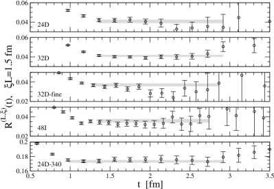
Figure 1: Results of $R^{(L,\xi)}(t)$ as a function of $t$. $R^{(L,\xi)}(t)$ are calculated using Eqs. (18) and (19). Here we have used the condition $\xi L=1.5$ fm.

Ensemble	New	Traditional
	$\langle r_{\pi}^{2}\rangle$ [fm2]	$\langle r_{\pi}^{2}\rangle$ [fm2]	$c_{V}$ [fm4]
24D	0.476(18)	0.466(30)	$-0.002(2)$
32D	0.480(10)	0.479(15)	$0.001(1)$
32D-fine	0.423(15)	0.409(28)	$0.001(2)$
48I	0.434(20)	0.395(32)	$-0.002(3)$
24D-340	0.3485(27)	0.3495(44)	0.0015(2)
PDG	0.434(5)

Table 2: Charge radii $\langle r_{\pi}^{2}\rangle$ from the new method by fitting $R^{(L,\xi)}(t)$ to a constant and from the traditional method by using the momentum extrapolation of $F_{\pi}(\hat{q}^{2})$. In the last row, the PDG value of $\langle r_{\pi}^{2}\rangle=0.434(5)$ Tanabashi et al. (2018) is listed for a comparison. This PDG value is obtained by combining the analysis of $e^{+}e^{-}\to\pi^{+}\pi^{-}$ data Ananthanarayan et al. (2017); Colangelo et al. (2019) and $\pi e\to\pi e$ data Dally et al. (1982); Amendolia et al. (1986); Gough Eschrich et al. (2001).

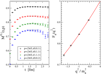
Figure 2: Using ensemble 24D-340 as an example, $M^{(L)}(t,\vec{p})$ as a function of $t$ are shown in the left panel and $F_{\pi}(\hat{q}^{2})$ as a function of $\hat{q}^{2}/m_{\pi}^{2}$ are shown in the right panel.

To make a comparison, we also calculate the charge radius using the tradition method. We perform the discrete spatial Fourier transform and calculate $\tilde{H}^{(L)}(t,\vec{p})$ using

$$\tilde{H}^{(L)}(t,\vec{p})=\frac{1}{N_{R}}\sum_{\hat{R}\in O_{h}}\sum_{\vec{x}\in\mathbb{L}^{3}}H^{(L)}(x)\cos[(\hat{R}\vec{p})\cdot\vec{x}].$$ (23)

where $N_{R}=\sum_{\hat{R}\in O_{h}}1$ and $O_{h}$ is the full cubic group for all lattice ratotations and reflections $\hat{R}$. We then construct the ratio

$$M^{(L)}(t,\vec{p})=\frac{\tilde{H}^{(L)}(t,\vec{p})}{\tilde{H}^{(L)}(t,\vec{0})}\frac{\tilde{E}}{\hat{E}}\frac{\hat{m}}{\tilde{m}}\frac{2\hat{m}}{\hat{E}+\hat{m}}e^{(E-m_{\pi})t}\doteq F_{\pi}(\hat{q}^{2}),$$ (24)

with $\vec{p}=\frac{2\pi}{L}\vec{n}$ for $\vec{n}=(0,0,1)$, $(0,1,1)$, $(1,1,1)$ and $(0,0,2)$. Here we use the ensemble 24D-340 with smallest statitical uncertainty as an example and show the $t$ dependence of $M^{(L)}(t,\vec{p})$ in the left panel of Fig. 2 as well as the $\hat{q}^{2}$ dependence of $F_{\pi}(\hat{q}^{2})$ in the right panel. We perform a correlated fit of the lattice data to a polynomial function

$$F_{\pi}(\hat{q}^{2})=1+\frac{1}{6}\langle r_{\pi}^{2}\rangle\hat{q}^{2}+c_{V}\left(\hat{q}^{2}\right)^{2}.$$ (25)

The fitting results are shown in Table 2. These results are consistent with the ones from the new method, but the errors are 1.5 - 1.9 times larger. Therefore, we use $\langle r_{\pi}^{2}\rangle$ from the new method in the following analysis.

Systematic effects. – To examine the finite-volume effects, we use the ensembles, 24D and 32D, which have the same pion mass and lattice spacing but different lattice sizes, $L=4.7$ and 6.2 fm. For these two ensembles, the results for $\langle r_{\pi}^{2}\rangle$ are very consistent, suggesting that the finite-volume effects are mild. This is not surprising since the coefficients $\beta_{k,n}^{(L,\xi)}$ in Eq. (17) are introduced to treat the finite-volume effects properly.

We have four ensembles nearly at the physical pion mass. The remaining systematic effects from the unphysical pion mass are small and can be corrected by using the information of the fifth ensemble, 24D-340, at $m_{\pi}\approx 340$ MeV. We adopt the chiral extrapolation formula Bijnens et al. (1998); Aoki et al. (2019) $\langle r_{\pi}^{2}\rangle=\frac{1}{(4\pi F_{0})^{2}}\left(-\ln\frac{m_{\pi}^{2}}{m_{\pi,\text{phys}}^{2}}+\kappa\frac{m_{\pi}^{2}}{(4\pi F_{0})^{2}}+\text{const}\right)$ with the constant term including the possible lattice artifacts. We fix $F_{0}=87$ MeV, a value estimated by using $F_{\pi}=92.2(1)$ MeV and $F_{\pi}/F_{0}=1.062(7)$ Aoki et al. (2019), and use the ensembles 24D, 32D and 24D-340 with the same lattice spacing to study the pion mass dependence. By extrapolating to the physical point, $\langle r_{\pi}^{2}\rangle$ for ensembles 24D, 32D, 32D-fine and 48I are shifted by $0.2$%, $0.3$%, $0.5$%, $-0.1$%, respectively. These changes are very small compared the statistical errors.

The largest systematic uncertainties in our study arise from the lattice discretization effects. The values of $\langle r_{\pi}^{2}\rangle$ for 24D and 32D are 13% larger than that for 32D-fine, suggesting a large lattice artifact. Unfortunately, the result from 48I cannot be used in the continuum extrapolation together with 24D, 32D and 32D-fine ones, as the 48I ensemble is simulated with Iwasaki gauge action, while the other three use Iwasaki+DSDR action. Considering the fact that 48I has the finest lattice spacing, we quote its value of $\langle r_{\pi}^{2}\rangle$ as the final result and attribute to it a $\sim 3$% discretization error by an order counting $O((a\Lambda_{\text{QCD}})^{2})$ with $\Lambda_{\text{QCD}}=300$ MeV

$$\langle r_{\pi}^{2}\rangle=0.434(20)(13)\text{ [fm${}^{2}$]}.$$ (26)

Note that the discretization error quoted here is a rough estimate. A further check of lattice artifacts using the finer lattice spacings is very necessary.

Conclusion. – We have used a model-independent method to calculate the hadron’s charge radius using lattice QCD. Given the hadronic function $H^{(L)}(x)$ from lattice QCD, we propose to calculate a physical quantity $O$ of interestes through the summation

$$O=\sum_{\vec{x}}\omega(\vec{x},t)H^{(L)}(\vec{x},t),\quad\mbox{for large $t$}.$$ (27)

Here the weight function $\omega(\vec{x},t)$ is analytically known and contains all the non-QCD information. In the calculation of the pion charge radius, where $O=\langle r_{\pi}^{2}\rangle$, we have introduced three different weight functions $\omega(\vec{x},t)$, which are encoded in the expressions of $R(t)$ in Eq. (7), $R^{(L)}(t)$ in Eq. (13) and $R^{(L,\xi)}(t)$ in Eq. (18). By choosing the appropriate weight function, we are able to reduce both systematic and statistical uncertainties. Such idea has been used in our earlier work on the calculation of QED self energies Feng and Jin (2019), and can be extended to the lattice computation of various processes such as $\pi^{0}\to\gamma\gamma$ decays.

In the calculation of the pion charge radius, our approach shows three peculiar features.

1. Simplicity: The method does not require the additional quark propagator inversion on twisted boundary conditions or sequential-source propagators with momentum derivatives. It does not require the modeling of the momentum dependence of the form factor. The charge radius can be simply extracted from $R^{(L,\xi)}(t)$ at large time separation to avoid the excited-state contamination.

2. Flexibility: In the whole calculation, it only requires the generation of the wall-source and point-source propagators. These propagators can be used to calculate other correlation functions in the future projects. Besides, the hadronic function $\langle 0|A_{\mu}(x)J_{\nu}(0)|\pi(\vec{0})\rangle$ constructed in this study can be used for other relevant physics processes, such as the radiative corrections to the pion’s decay.

3. Precision: The statistical uncertainties of $\langle r_{\pi}^{2}\rangle$ from the new method are about 1.5 - 1.9 smaller times than that from the traditional method. We expect the method is more efficient in the nucleon sector where the hadronic function near the boundary of box contributes significant noise. Besides for the reduction of the statistical uncertainty, the model dependence from the choices of the fit ansatz is also avoided by using the new method.

In this study, we find that the largest source of the uncertainty is from the lattice discretization. This can be controlled by using gauge configurations with finer lattice spacings and performing the continnum extrapolations. With the developments of supercomputers, technologies as well as the new ideas and methods, we can foresee that in the near future lattice QCD calculations can provide the determinations of $\langle r_{\pi}^{2}\rangle$, which has the similar precision as the current PDG value or even surpasses it. These developments also shed the light on precise determinations of the proton charge radius from first-principle theory that can distinguish between the conflicting experimental values.

I Acknowledgments

We gratefully acknowledge many helpful discussions with our colleagues from the RBC-UKQCD Collaborations. X.F. and Y.F. were supported in part by NSFC of China under Grant No. 11775002. L.C.J. acknowledges support by DOE grant DE-SC0010339. The computation is performed under the ALCC Program of the US DOE on the Blue Gene/Q (BG/Q) Mira computer at the Argonne Leadership Class Facility, a DOE Office of Science Facility supported under Contract DE-AC02-06CH11357. The calculation is also carried out on Tianhe 3 prototype at Chinese National Supercomputer Center in Tianjin.

References

- Pohl et al. (2010) R. Pohl et al., Nature 466, 213 (2010).
- Bezginov et al. (2019) N. Bezginov, T. Valdez, M. Horbatsch, A. Marsman, A. C. Vutha, and E. A. Hessels, Science 365, 1007 (2019).
- Xiong et al. (2019) W. Xiong, A. Gasparian, H. Gao, et al., Nature 575, 147 (2019).
- Bedaque (2004) P. F. Bedaque, Phys. Lett. B593, 82 (2004), arXiv:nucl-th/0402051 [nucl-th] .
- de Divitiis et al. (2004) G. M. de Divitiis, R. Petronzio, and N. Tantalo, Phys. Lett. B595, 408 (2004), arXiv:hep-lat/0405002 [hep-lat] .
- de Divitiis et al. (2012) G. M. de Divitiis, R. Petronzio, and N. Tantalo, Phys. Lett. B718, 589 (2012), arXiv:1208.5914 [hep-lat] .
- Hasan et al. (2018) N. Hasan, J. Green, S. Meinel, M. Engelhardt, S. Krieg, J. Negele, A. Pochinsky, and S. Syritsyn, Phys. Rev. D97, 034504 (2018), arXiv:1711.11385 [hep-lat] .
- Brömmel et al. (2007) D. Brömmel et al. (QCDSF/UKQCD), Eur. Phys. J. C51, 335 (2007), arXiv:hep-lat/0608021 [hep-lat] .
- Aoki et al. (2009) S. Aoki et al. (JLQCD, TWQCD), Phys. Rev. D80, 034508 (2009), arXiv:0905.2465 [hep-lat] .
- Wang et al. (2018) G. Wang, J. Liang, T. Draper, K.-F. Liu, and Y.-B. Yang, Proceedings, 36th International Symposium on Lattice Field Theory (Lattice 2018): East Lansing, MI, United States, July 22-28, 2018, PoS LATTICE2018, 127 (2018), arXiv:1810.12824 [hep-lat] .
- Frezzotti et al. (2009) R. Frezzotti, V. Lubicz, and S. Simula (ETM), Phys. Rev. D79, 074506 (2009), arXiv:0812.4042 [hep-lat] .
- Boyle et al. (2008) P. A. Boyle, J. M. Flynn, A. Juttner, C. Kelly, H. P. de Lima, C. M. Maynard, C. T. Sachrajda, and J. M. Zanotti, JHEP 07, 112 (2008), arXiv:0804.3971 [hep-lat] .
- Nguyen et al. (2011) O. H. Nguyen, K.-I. Ishikawa, A. Ukawa, and N. Ukita, JHEP 04, 122 (2011), arXiv:1102.3652 [hep-lat] .
- Brandt et al. (2013) B. B. Brandt, A. Jüttner, and H. Wittig, JHEP 11, 034 (2013), arXiv:1306.2916 [hep-lat] .
- Aoki et al. (2016) S. Aoki, G. Cossu, X. Feng, S. Hashimoto, T. Kaneko, J. Noaki, and T. Onogi (JLQCD), Phys. Rev. D93, 034504 (2016), arXiv:1510.06470 [hep-lat] .
- Koponen et al. (2016) J. Koponen, F. Bursa, C. T. H. Davies, R. J. Dowdall, and G. P. Lepage, Phys. Rev. D93, 054503 (2016), arXiv:1511.07382 [hep-lat] .
- Alexandrou et al. (2018) C. Alexandrou et al. (ETM), Phys. Rev. D97, 014508 (2018), arXiv:1710.10401 [hep-lat] .
- Meyer (2011) H. B. Meyer, Phys. Rev. Lett. 107, 072002 (2011), arXiv:1105.1892 [hep-lat] .
- Feng et al. (2015) X. Feng, S. Aoki, S. Hashimoto, and T. Kaneko, Phys. Rev. D91, 054504 (2015), arXiv:1412.6319 [hep-lat] .
- Erben et al. (2019) F. Erben, J. R. Green, D. Mohler, and H. Wittig, (2019), arXiv:1910.01083 [hep-lat] .
- Bouchard et al. (2016) C. Bouchard, C. C. Chang, K. Orginos, and D. Richards, Proceedings, 34th International Symposium on Lattice Field Theory (Lattice 2016): Southampton, UK, July 24-30, 2016, PoS LATTICE2016, 170 (2016), arXiv:1610.02354 [hep-lat] .
- Aglietti et al. (1994) U. Aglietti, G. Martinelli, and C. T. Sachrajda, Phys. Lett. B324, 85 (1994), arXiv:hep-lat/9401004 [hep-lat] .
- Lellouch et al. (1995) L. Lellouch, J. Nieves, C. T. Sachrajda, N. Stella, H. Wittig, G. Martinelli, and D. G. Richards (UKQCD), Nucl. Phys. B444, 401 (1995), arXiv:hep-lat/9410013 [hep-lat] .
- Note (1) We thank C. C. Chang for raising this point to us.
- Blum et al. (2016) T. Blum et al. (RBC, UKQCD), Phys. Rev. D93, 074505 (2016), arXiv:1411.7017 [hep-lat] .
- Mawhinney (2018) R. Mawhinney, in Proceedings, The 36th Annual International Symposium on Lattice Field Theory (LATTICE2018) (2018).
- Tanabashi et al. (2018) M. Tanabashi et al. (Particle Data Group), Phys. Rev. D98, 030001 (2018).
- Ananthanarayan et al. (2017) B. Ananthanarayan, I. Caprini, and D. Das, Phys. Rev. Lett. 119, 132002 (2017), arXiv:1706.04020 [hep-ph] .
- Colangelo et al. (2019) G. Colangelo, M. Hoferichter, and P. Stoffer, JHEP 02, 006 (2019), arXiv:1810.00007 [hep-ph] .
- Dally et al. (1982) E. B. Dally et al., Phys. Rev. Lett. 48, 375 (1982).
- Amendolia et al. (1986) S. R. Amendolia et al. (NA7), Proceedings, 23RD International Conference on High Energy Physics, JULY 16-23, 1986, Berkeley, CA, Nucl. Phys. B277, 168 (1986).
- Gough Eschrich et al. (2001) I. M. Gough Eschrich et al. (SELEX), Phys. Lett. B522, 233 (2001), arXiv:hep-ex/0106053 [hep-ex] .
- Bijnens et al. (1998) J. Bijnens, G. Colangelo, and P. Talavera, JHEP 05, 014 (1998), arXiv:hep-ph/9805389 [hep-ph] .
- Aoki et al. (2019) S. Aoki et al. (Flavour Lattice Averaging Group), (2019), arXiv:1902.08191 [hep-lat] .
- Feng and Jin (2019) X. Feng and L. Jin, Phys. Rev. D100, 094509 (2019), arXiv:1812.09817 [hep-lat] .