Measuring the Time-Varying Market Efficiency
in the Prewar Japanese Stock Market, 1924–1943

Abstract: This study explores the time-varying structure of market efficiency for the prewar Japanese stock market using a new market capitalization-weighted stock price index based on the adaptive market hypothesis (AMH). First, we find that the degree of market efficiency in the prewar Japanese stock market varies over time and with major historical events. Second, the AMH is supported in this market. Third, this study concludes that market efficiency was maintained throughout the period, whereas previous studies did not come to the same conclusion due to differences in the calculation methods of stock indices. Finally, as government intervention in the market intensified throughout the 1930s, the market efficiency declined, as well as rapidly taking into account the war risk premium, especially from the time when the Pacific War became inevitable.

Keywords: Efficient Market Hypothesis; Adaptive Market Hypothesis; GLS-Based Time-Varying Model Approach; Price Control Policy; War Risk Premium.

JEL Classification Numbers: C22; G12; G14; N20.

1 Introduction

Economists have shown interest in assessing whether the efficient market hypothesis (EMH) proposed by Fama’s (1970) is applicable to stock markets. However, there is no consensus on its applicability to stock markets, which is why the hypothesis remains controversial, as described by Malkiel (2004) and Shiller (2005). As such, Lo (2004) proposes the adaptive market hypothesis (AMH) as an alternative to the EMH. The AMH asserts that market efficiency may fluctuate over time and the fluctuations may be due to several factors, including context, market participants, microstructure, and behavioural biases. In other words, the main argument of the AMH is that it is not realistic to enquire whether the market is completely efficient as per the EMH. Indeed, Lo (2004) shows that market efficiency has cyclically changed over time, with surprising evidence that the U.S. stock market was more efficient in the 1950s than in the early 1990s.

In an overview of the literature on the AMH, Lim and Brooks (2011) show that various methods, time-varying parameter models, and conventional statistical inferences with rolling window, have been employed to explore whether the stock market and market efficiency change over time. Previous studies also detect the periods when the market has been inefficient to explore whether business cycles, bubbles, and economic crises in financial markets have specific dynamics and clarify whether their evolution determines such market dynamics, as mentioned by Lo (2005). Studies such as Ito and Sugiyama (2009), Ito et al. (2014, 2016), Kim et al. (2011), Lim et al. (2013), and Noda (2016) affirm that stock markets evolve over time in accordance with the changes in market conditions. However, there are few studies on stock market efficiency from a historical perspective, owing to low availability of prewar stock market data (except for the U.S. and Japan).

Two major long-run datasets exist for the prewar U.S. stock market: the Dow Jones Industrial Average index and the S&P composite index. Choudhry (2010) investigates endogenous structural breaks in the U.S. stock market using the daily Dow Jones Industrial Average index during World War II (WWII) and Perron’s (1997) structural shift-oriented test. He concludes that the market’s breakpoints are consistent with major historical events during the war. Kim et al. (2011) applies the daily Dow Jones Industrial Average index from 1900 to 2009 to examine time-varying return predictability using automatic variance ratio-based test statistics. They find compelling evidence of return predictability changes over time and its association with stock market volatility and economic fundamentals. This is consistent with the implications of the AMH. By employing the monthly S&P composite index from 1871 to 2012 along with a generalised least square (GLS)-based time-varying autoregressive (AR) model, Ito et al. (2016) conclude that market efficiency and the U.S. stock market change over time, confirming the application of the AMH to the U.S. stock market.

Unlike the prewar U.S. stock market, there is no composite stock market index for the prewar Japanese stock market. In other words, previous studies employ various non composite stock market indexes to examine whether the prewar Japanese stock market has been efficient in the context of the EMH. Kataoka et al. (2004) employ daily stock prices for 1900 and calculate autocorrelation coefficients, finding that the market was almost efficient in the weak sense, as conceptualised by Fama (1970). Suzuki (2012) uses the breakpoints estimated by Choudhry (2010) and daily stock market data to investigate their relationship with major historical events during the Pacific War and the variation in stock prices, respectively. Suzuki (2012) concludes that market efficiency declined after the beginning of the Pacific War because of that the war risk premium of Reitz (1988) and Barro (2006) was reflected promptly in the price formation process. Bassino and Lagoarde-Segot (2015) use the simple arithmetic average of daily stock prices from 1931 to 1940, along with Engle et al.’s (1987) generalised AR conditional heteroskedasticity-in-mean (GARCH-in-mean) model to investigate information efficiency in the prewar Japanese stock market. Although they find that the Japanese stock market deviated from weak-form efficiency in the 1930s, their price index does not include the shares of the Tokyo Stock Exchange (TSE), which accounts for the largest shares in terms of trading volume and, thus, does not appropriately represent the price trends of the prewar Japanese stock market. Therefore, previous studies have employed stock prices per industry or a volume-weighted price index as datasets, along with somewhat unsophisticated empirical methods. Moreover, the sample periods in most studies are too short to examine whether the modem stock market evolves and market efficiency changes over time in accordance with the AMH. It is obvious that those price indexes cannot accurately reflect the performance of the stock market.

The prevailing view in Japanese economic history is that the stock market during wartime stagnated due to wartime control. Indeed, as Okazaki (1999) points out, based on money flow data, the corporate funding function of the stock market has regressed. However, even after the end of the 1930s, when wartime economic controls were tightened, the stock market’s volatility and liquidity remained at a certain level. As for the wartime period, Hirayama (2018, 2020, 2022) point out that the volatility of the stock returns was still over 10% while the variation of returns on the Japanese government bond market disappeared. Therefore, it could not be considered that the pricing function in the stock market had disappeared. At that time, the Japanese stock market, which was mostly clearing future transactions that did not require cash equivalent, could keep its pricing function separate from the flow of funds. We thus consider the functions of corporate financing and pricing in the stock market separately and conclude that market efficiency must be verified for the functions of pricing in the stock market as a whole during wartime. Specifically, we examine market efficiency based on Suzuki’s (2012) conclusion that the existence of a war risk premium declined market efficiency and Lo’s (2004) adaptive market hypothesis, taking into account investors’ risk attitudes.

In other words, this study examines the interrelationship between the time-varying nature of market efficiency and historical events in the prewar Japanese stock market from the perspective of the AMH. Our examination is fourfold. First, we provide a historical review of the datasets used in previous studies from the viewpoint of sample periods and data adequacy and pinpoint the problems of these datasets. Second, we introduce an accurate performance index of the prewar Japanese stock market from 1924 to 1945 constructed by Hirayama (2018, 2020). We confirm that our new dataset reflects the price behaviour of the Japanese stock market in the prewar period accurately (the period verified in this paper is from June 1924 to June 1943, when deferred fee data for short-term clearing transactions are available). Third, we examine whether the modem stock market evolved and market efficiency changed over time in accordance with Lo’s (2004) AMH. At this stage, we measure the degree of market efficiency, taking into account investors’ risk attitudes, with statistical inferences using Ito et al.’s (2014; 2022) GLS-based time-varying parameter model. This approach is superior to the conventional statistical tests used in previous studies, such as Kim et al.’s (2011) automatic variance ratio test using moving-window samples; in other words, it is independent of sample size. Finally, we investigate the relationships between major historical events and the variations in market efficiency using one of the most reliable primary sources–the Bank of Japan’s Monthly Survey, The Monthly Survey is more reliable than other sources for interpreting the variation of market efficiency, because it is written in a unified format and ensured data continuity. We reliably detect when the efficiency of the prewar Japanese stock market increased or declined over time and, thus, investigate the possibility that historical events have affected market efficiency.

The remainder of the paper is organised as follows. Section 2 describes the prewar Japanese stock market and confirms the adequacy of the datasets used in previous studies. Section 3 presents the empirical methodology for estimating the degree of market efficiency based on Ito et al.’s (2014; 2022) GLS-based time-varying parameter model. Section 4 presents the new dataset of price indexes for the prewar Japanese stock market estimated by Hirayama (2018, 2020), and the results of selected statistical tests. Section 5 shows the empirical results using GLS-based time-varying parameter models and discusses the relationships between major historical events and time-varying market efficiency in the prewar Japanese stock market. Section 6 concludes the paper.

2 A Historical Review of the Prewar Japanese Stock Market

Here, we describe the characteristics of the prewar Japanese market, including the types and methods of transactions and the stock market index.

2.1 Stock Market Centred on Non-Deliverable Trading

In the prewar period, there were three types of trading methods on stock exchanges: spot transactions (jitsubutu torihiki), long-term clearing futures transactions (choki seisan torihiki), and short-term clearing futures transactions (tanki seisan torihiki). While spot transactions assumed stock delivery, long- and short-term clearing futures transactions focused on non-deliverable trading. As Figure 1 shows, spot transactions did not exceed 10% of all transactions on the TSE (Tokyo Stock Exchange; the largest stock exchange in prewar Japan and the TSE itself was a listed stock company), until the end of the 1930s, with futures transactions accounting for the majority.

(Figure 1 around here)

In particular, the proportion of transactions related to TSE’s new shares, was high, such as major issues of short-term futures; further, the share of short-term futures transactions increased to 81% in November 1938. Therefore, the market was dominated by highly liquid short-term futures transactions until the end of the 1930s. The positioning of TSE’s new shares (short-term clearing only) in long-term clearing and short-term clearing trades on the Tokyo Stock Exchange was as follows. On average during the period from 1928 to 1942, the market capitalization ratio was only 1.1%, but the trading volume accounted for 45.5%. Therefore, TSE’s new shares should be taken into consideration when examining prewar and wartime stock markets. At the same time, if we place too much emphasis on trading volume share, it becomes difficult to see the characteristics of other stocks, so we need to be careful. In December 1941, when the Pacific War broke out, the share of short-term clearing futures transactions declined. Finally, the TSE was unlisted on 31 August 1943 and the exchanges in various regions were consolidated into the Japan Stock Exchange. Accordingly, short-term clearing futures transactions were abolished and stock transactions were conducted through long-term clearing futures and spot transactions.

While shares were delivered for spot transactions, the rate of delivery was low in the case of long- and short-term clearing futures transactions, as most were net settlements. An increase in non-deliverable trading relative to the settlements associated with the transfer of shareholders can be considered an indicator of increased market pricing function and liquidity.

2.2 Methods for Stock Price Index Calculation and Market Characteristics in the Early Showa Period

Short-term clearing futures transactions comprised the core of the Japanese stock market in the early Showa period. The initially listed stocks were limited to TSE’s and Kanegafuchi Spinning’s new shares. As other issues were added to the short-term clearing futures transactions, the effect of two specified stocks trading on the market capitalization-weighted average index decreased. However, as the trading volume of these stocks accounted for the majority of transactions until 1942, the effect of specific share’s trading on the index weighted by trading volume remained strong. There is a difference in the characteristics of stock markets based on a market capitalization index versus a trading volume index. Notably, most stock indexes created during the early Showa period were trading-volume weighted averages or simple averages, while the current stock index is generally based on the market capitalization-weighted average.

The trading-volume weighted average was too greatly affected by the price fluctuations of some stocks with high trading volumes (TSE’s and Kanegafuchi Spinning’s new shares) to represent the overall performance of the stock market. For example, the Kabuka Dai-Shisu (stock price index) calculated by the TSE using Fisher’s (1921) formula which is one of the methods for calculating the consumer price index according to transaction volume and the Zen-Sango Shin-Kyu Sogo Kabuka Shisu (all-industry old and new composite stock price index) conducted by Fujino and Akiyama (1977) are weighted average indexes based on trading or settlement volume. Therefore, the effect of TSE’s new shares was significant and the effect of excessive concentrative trading cannot be eliminated. Consequently, to understand the characteristics of the overall stock market, it is necessary to dilute the excessive effects of some stocks, such as TSE’s new shares.

Meanwhile, the influence of stocks with small market capitalization and low liquidity is undeniably greater than that of the capitalization-weighted type for an index based on simple averages. The Stock Price Index calculated by the Bank of Japan and Daily Stock and Government Bond Price Index calculated by the Toyo Keizai Shimpo—adopted by Bassino and Lagoarde-Segot (2015)—are indexes based on simple averages. As such, they can be used to eliminate the effects of TSE’s new shares. However, as the ratio of small-cap stocks was relatively high and the impact of large -cap stocks might be underestimated, it is important to capture the overall stock market adequately.

This study uses the Equity Performance Index (EQPI), which is a capitalization- weighted average index for short-term clearing futures transactions. We recognise that spot transactions and long-term clearing futures transactions—with relatively low trading volumes per share owing to many listed companies and issues—are not appropriate for tracking secondary market conditions. Although the ratio of highly specific stocks was high during the initial phase of the EQPI, the effect of TSE’s and Kanegafuchi Spinning’s new shares gradually decreased. Additional industrial stocks were adopted, which reflects the characteristics of the prewar Japanese stock market. The characteristics of the EQPI index changed over time, because the number of listed companies and issues was limited.

As previously described, the prewar stock index in Japan reflected a market structure wherein market characteristics were easily influenced by the calculation method employed. Therefore, it is necessary to examine the index after clearly understanding these characteristics. Previous studies on market efficiency do not consider the microstructure of the stock market. Consequently, it may be necessary to examine every aspect of index characteristics to verify efficiency. In what follows, we examine changes in the characteristics of the stock market by the index calculation method from two aspects: changes in the description of market trends (focus points by market participants) in the Bank of Japan’s Monthly Survey and changes in the deferment fees for the settlement of differences in short-term clearing transactions.

First, to confirm whether the characteristics of the stock market changed, it is important to identify the market’s characteristics from the description changes in the using stock market trends mentioned in the Monthly Survey, especially for the early Showa period. The Monthly Survey is a more reliable data source than newspapers because it is a market survey conducted by a public organisation, is presented in a consistent format, and has been conducted over a long period of time. In this study, the sample period comprises 203 months from June 1924 to April 1941. We classify the market fluctuation factors under the “Stock Market” column in the Monthly Survey into 14 categories and confirm their changing nature over time, as shown in Table 1.

(Table 1 around here)

From the Monthly Survey, we can confirm the fact that the TSE’s and Kanegafuchi Spinning’s new shares attracted more attention during certain periods. Additionally, there were periods wherein the selection of stocks focused on investment attractiveness, such as the profitability of stock dividend yields relative to bond yields. Specifically, extreme increases (bubble phenomenon) or falls (collapse phenomenon) in the stock market were related to the concentration of specific share transactions, such as TSE’s new shares and the diffusion of transactions to many industrial stocks. Previous studies have attempted to examine the Japanese stock market’s efficiency on a temporary or full-year basis. Given that prewar stock markets in Japan were characterised by a high market share of highly liquid TSE’s new shares, it is important to understand that the periods of overheating and stagnation differ depending on the method of calculating the index.

Second, we can understand the time-based changes in market characteristics by examining the changing deferment fees for the EQPI (weighted average market capitalization). Based on changes in the negative and positive deferment fee, we could determine when the distortions in the stock supply and demand occur in the stock market.

A rule for short-term clearing futures transactions was to transfer the payments and share certificates simultaneously with trading (same-day delivery for transactions processed on the previous day’s afternoon and the current day); however, it was possible to defer delivery and settlement through a deferment fee. The deferral agencies executed delivery on behalf of all sellers and buyers. Specifically, when excessive shares had to be delivered, payment was made on behalf of the purchaser and excess shares were received (cash transfer); and when there was a shortage of shares, the shortfall was covered on behalf of the seller and payment was received (stock transfer). Since the deferment agency decided the deferment fee based on the bias of the trading position, the level was regarded as one of the indicators of the overall market situation. Specifically, the deferment fee was determined by the market interest rate, the deferral conditions of the trading member, and the agency’s willingness to adjust delivery. The decisive factor was the amount of stock that could be delivered. Deferment agencies intentionally increased deferment fee to adjust for the bias in deferred deliveries by market participants. For this reason, it was assumed that the positive deferment fee would be set at a high rate when the number of shares on the buy side increased rapidly, and the negative deferment fee would be set at a high rate when the number of shares on the sell side increased rapidly.

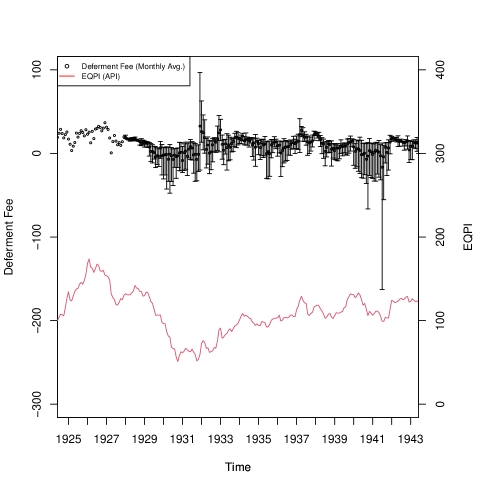
Figure 2: Deferment Fee on Short-Term Futures Transactions (All Stocks Weighted)

(Figure 2 around here)

Figure 2 shows the weighted average of the deferment fees for all stocks in the short-term clearing futures transactions market . The average monthly deferment fee for the period examined in this study is around 11 sen ($=0.11$ yen), which is lower than that for TSE’s new shares (20 sen). In the early Showa period, negative deferment fees were observed for all issues of short-term clearing futures transactions (weighted average market capitalization), mainly in two periods:(1) from the Showa Depression to the lifting of the ban on gold exports (from August 1929 to October 1930); and (2) around July 1941, when the rapid deterioration became evident compared with the U.S. and the assets held by Japan were frozen by the U.S. Compared.

Meanwhile, positive deferment fees rose sharply in four periods: (3) in December 1926, when buying speculation with respect to buying Kuhara Mining shares reached its peak after November 1926; (4) after December 1931, when the new Cabinet of Prime Minister Tsuyoshi Inukai (Minister of Finance Korekiyo Takahashi) promulgated the ban on gold exports and announced additional payment of the TSE’s new shares, causing the stock market to soar (from December 1931 to March 1932); (5) from December 1932 to January 1933, when expectations of monetary easing grew and stock exchanges recorded the trading volume after the Bank of Japan began underwriting government bonds amid the appreciation of the U.S. dollar; and (6) after March 1937, when the TSE recorded its highest trading volume before the war. When the positive deferment fee was high, fluctuation was relatively limited. However, in December 1931, it reached 97 sen ($=0.97$ yen). Thus, it could be assumed that a temporary increase in the deferment fee was implemented to tackle panic buying. Therefore, we can confirm the following based on the information above: In the early Showa period, the concentration of unidirectional transactions occurred around the Showa depression during a series of policy changes for lifting the ban on and re-prohibition of gold exports.

High market liquidity will be required in order to vividly confirm the imbalance and leveling of supply and demand caused by external conditions and internal market factors. Since such external information can be reflected in short-term clearing transactions, which can be bought and sold flexibly and easily through the exchange of deferment fees, ensuring liquidity should be given priority in verifying market efficiency. As noted above for changes in deferment fees, highly liquid short-term clearing transactions provided this condition. However, indexes based on investment performance in spot and long-term clearing transactions did not have this condition and are therefore not suitable for efficiency testing. In addition, even for a stock index for short-term clearing transactions, the impact of TSE’s new share on the trading volume weighted average was excessively large, so the calculation of the index by the market capitalization weighted average would be required.

As described above, in addition to the characteristics of the stock index, the market characteristics of the pre-war period were confirmed multilaterally from aspects such as the concentration of trading issues based on monthly survey and the perception of market participants, as well as changes supply and demand distortions based on deferred changes for short-term clearing transactions. As a result, it became clear that the characteristics of the Japanese stock market changed significantly from the early Showa period to the wartime period, and it is appropriate to examine market efficiency using a market capitalization weighted average stock index for short-term clearing transactions. In what follows, we will examine whether the efficiency of the stock market is also affected and changed by market conditions.

3 The Model

This section briefly reviews Ito et al.’s (2014; 2022) GLS-based time-varying parameter model. To obtain the degree of market efficiency of the prewar Japanese stock market in each period using multivariate data, we employ a special case of their model—a GLS-based time-varying vector autoregressive (TV-VAR) model. The model allows us to understand the interrelationships among variables that cannot be considered in the TV-VAR model, such as the relationship between stock returns and investors’ risk attitudes. Then, we examine the market function’s time-varying nature.

Suppose ${{\mbox{\boldmath$p$}}_{t}}$ is a price vector of the stock and deferment fee in $t$ period. We focus on the following condition defined by Fama (1970):

$${\mathbb{E}}\left[{{\mbox{\boldmath$x$}}_{t}}\mid\mathcal{I}_{t-1}\right]={\mbox{\boldmath$0$}},$$ (1)

where ${\mbox{\boldmath$x$}}_{t}$ is a return vector of the stock price and deferment fee in $t$ period. We calculate that the $i$-th element of ${{\mbox{\boldmath$x$}}_{t}}$ is $\ln{p_{i,t}}-\ln{p_{i,t-1}}$ for each variable. In other words, the expected returns of the stock and deferment fee at time $t$ given the information set available at time $t-1$ is $\mathrm{𝟎}$. When ${\mbox{\boldmath$x$}}_{t}$ is stationary, Wold decomposition is used to formulate the time-series process of ${\mbox{\boldmath$x$}}_{t}$ as follows:

$${\mbox{\boldmath$x$}}_{t} = {\mbox{\boldmath$\mu$}}+\Phi_{0}{\mbox{\boldmath$u$}}_{t}+\Phi_{1}{\mbox{\boldmath$u$}}_{t-1}+\Phi_{2}{\mbox{\boldmath$u$}}_{t-2}+\cdots$$ (2)

$$= {\mbox{\boldmath$\mu$}}+\Phi(L){\mbox{\boldmath$u$}}_{t},$$

where $\Phi(L)$ is a matrix lag polynomial of a lag operator, $\mu$ is the mean of ${\mbox{\boldmath$x$}}_{t}$, and ${\mbox{\boldmath$u$}}_{t}$ follows an independent and identically distributed multivariate process with a mean of zero vector. And we assume that coefficient matrices $\{\Phi_{i}\}^{\infty}_{i=0}$ are $k\times k$ dimensional parameter matrices. Then We compute the impulse response functions along with the identification assumptions such as $\Phi_{0}=I$. This suggests that the deviation from an efficient market reflects an impulse response, which is a series of $\{{\mbox{\boldmath$u$}}_{t}\}$. we construct an index based on the impulse response to investigate whether the EMH is supported or not in the prewar Japanese stock market. The impulse response can be easily obtained by using an VAR model and algebraically computing its estimates. We find that the process of the return of stock price and deferment fee $x$ is invertible under some conditions. Then, we consider the following standard VAR($q$) model:

$${\mbox{\boldmath$x$}}_{t}={\mbox{\boldmath$\nu$}}+A_{1}{\mbox{\boldmath$x$}}_{t-1}+A_{2}{\mbox{\boldmath$x$}}_{t-2}+\cdots+A_{q}{\mbox{\boldmath$x$}}_{t-q}+{\mbox{\boldmath$\varepsilon$}}_{t};\ \ t=1,2,\ldots,T,$$ (3)

where $\nu$ is a vector of intercepts; ${\mbox{\boldmath$\varepsilon$}}_{t}$ is a multivariate error term with ${\mathbb{E}}\left[{\mbox{\boldmath$\varepsilon$}}_{t}\right]={\mbox{\boldmath$0$}}$,  ${\mathbb{E}}\left[{\mbox{\boldmath$\varepsilon$}}_{t}^{2}\right]=\sigma_{{\mbox{\boldmath$\varepsilon$}}}^{2}I$, and ${\mathbb{E}}\left[{\mbox{\boldmath$\varepsilon$}}_{t}{\mbox{\boldmath$\varepsilon$}}_{t-m}\right]={\mbox{\boldmath$0$}}$ for all $m\neq 0$. We can measure a relative degree about the market efficiency that varies over time according to the following procedure. First, we compute a cumulative sum of the coefficient matrices of the impulse response:

$$\Phi(1)=\left(I-A_{1}-A_{2}-\cdots-A_{q}\right)^{-1},$$ (4)

Then we define the degree of market efficiency as follows:

$$\zeta=\sqrt{\mbox{max}\left[(\Phi(1)-I)^{\prime}(\Phi(1)-I)\right]},$$ (5)

to measure the deviation from the efficient market. We can understand that in the case of the efficient market where $A_{1}=A_{2}=\cdots=A_{q}=0$, the degree $\zeta$ becomes zero; otherwise, $\zeta$ deviates from zero. Hence, we regard $\zeta$ as the degree of market efficiency. We consider a large deviation of $\zeta$ from $0$ (either positive or negative) as evidence of market inefficiency. Moreover, we can construct time-based changes in the degree when we obtain time-varying estimates of the coefficients in Equation (3).

We estimate TV-VAR coefficients for each period to obtain the corresponding degree defined in Equation (5). Following this method, we use a model wherein all the VAR coefficients, except the one corresponding to the intercept terms, $\nu$, follow independent random walk processes. In other words, we suppose

$$A_{l,t}=A_{l,t-1}+V_{l,t},\ \ (l=1,2,\cdots,q),$$ (6)

where $\{V_{l,t}\}$ is a $q\times t$ dimensional error term matrix. We assume that the matrix satisfies $E\left[V_{l,t}\right]={\mbox{\boldmath$O$}}$ for all $t$,  $E\left[vec(V_{l,t})^{\prime}vec(V_{l,t})\right]=\sigma_{v}^{2}I$ and $E\left[vec(V_{l,t})^{\prime}vec(V_{l,t-m})\right]={\mbox{\boldmath$O$}}$ for all $l$ and $m\neq 0$. Ito et al.’s (2014; 2022) method allows us to estimate the following GLS-based TV-VAR model:

$${\mbox{\boldmath$x$}}_{t}={\mbox{\boldmath$\nu$}}+A_{1,t}{\mbox{\boldmath$x$}}_{t-1}+A_{2,t}{\mbox{\boldmath$x$}}_{t-2}+\cdots+A_{q,t}{\mbox{\boldmath$x$}}_{t-q}+{\mbox{\boldmath$\varepsilon$}}_{t},$$ (7)

together with Equation (6).

Furthermore, we apply a residual bootstrap technique to the TV-VAR model to conduct statistical inference for the time-varying degree of market efficiency. Based on the hypothesis that all the TV-VAR coefficients are $0$, we formulate a set of bootstrap samples for the TV-VAR estimates. Assuming that the processes for all variables are generated under the efficient market hypothesis, this procedure provides us with a (simulated) distribution of the estimated TV-VAR coefficients. Then, we compute the corresponding distributions of the impulse response and degree of market efficiency. Finally, we conduct statistical inference for the estimates to examine whether the AMH is supported or not in the prewar Japanese stock market. In particular, we detect periods when the prewar Japanese stock market experienced market inefficiency by using confidence bands derived from such simulated distributions.

4 Data

We use the EQPI—the first capitalization-weighted index—of the prewar Japanese stock market, calculated by Hirayama (2018, 2020). Bassino and Lagoarde-Segot (2015), a representative study, use a daily dataset from the Japanese yearbooks of Toyo Keizai Shimpo (Oriental Economist). In the period from January 1931 to December 1940 covered by Bassino and Lagoarde-Segot (2015),the performance of EQPI was 55.9% for PI and 57.0% for API, confirming that the impact of correction of ex-right and additional payments was moderate. Also, the volatility (annualized value of monthly standard deviation) over the same period was 17.0% for PI and 16.5% for API, showing that these corrections had a significant impact. Japan’s stock investment performance in the prewar period requires various adjustments to the rate of change in stock prices, and this point should not be taken lightly when examining market efficiency.

On the other hand, the EQPI is a market capitalization-weighted average that adjusts the share price by issuing new shares or making other payments Hirayama (2018, 2020) calculates not only the price index and adjusted price index, but also the total return index, which considers the effect of dividends. Ideally, the total return index is desirable for expressing investors’ stock investment performance.

(Table 2 around here)

Table 2 demonstrates the differences between well-known stock price indexes and the EQPI of prewar Japan. Tokyo Stock Exchange used a volume-weighted average to calculate its stock index. In addition, Toyo Keizai Shimpo and Nippon Kangyo Bank used simple averages to calculate their stock indexes, but there are few market-weighted stock indexes, the same method used today. Furthermore, there is no stock index that takes into account the impact of new share allocation and other corporate actions (including dividends) on investment performance. We can understand the value of capital in the prewar Japanese stock market using the capitalization-weighted index. We believe that EQPI is appropriate for examining the stock market in Japan during the prewar period, based on the following four points: (1) TSE’s new shares, which represent the stock market before the war, are subject to EQPI; (2) EQPI is a market capitalization-weighted index, which is also used in modern stock indices, making it more comparable to modern ones; (3) EQPI is an index in which the impact of new share allocation and additional payments on investment performance has been appropriately modified; and (4) EQPI is a total return index that includes dividends and accurately reflects investment performance.

We use three types of monthly average price indexes for the EQPI: the price index (PI), adjusted price index (API), and total return index (TRI). Moreover, we employ the deferment fees as a proxy variable for investors’ risk attitudes because if the market is efficient, the deferment fees are also determined efficiently. The sample periods of each variable are the same, from June 1924 to June 1943. We log the first differences of the price or fee time series to obtain the indices’ returns.

(Table 3 around here)

Table 3 presents the descriptive statistics of the variables. The mean of returns on the total return index is higher than the price and adjusted price indices. It implies that the income gain is higher than the capital gain in the prewar Japanese stock market; therefore, we must consider dividends. On the other hand, we can see that the volatility of the changes in the deferment fees is extremely high, which means that the deferment agency reacted sensitively to the changes in the market environment and often change their risk attitudes. We believe that it can be used as a proxy variable for investors’ risk sensitivity since the rate of change in the deferment fee tends to increase as supply and demand in the short-term clearing market become more biased. Thus we should take into account the the possibility that the changes is determined simultaneously with the stock returns in our VAR estimation.

Table 3 includes the results of the unit root test with descriptive statistics. For estimation, all variables that appear in the moment conditions should be stationary. We apply the augmented Dickey–Fuller GLS (ADF-GLS) test of Elliott et al. (1996) to confirm whether the variables satisfy the stationarity condition. Furthermore, we employ the modified Bayesian information criterion instead of the modified Akaike information criterion to determine the optimal lag length. This is because the estimated coefficient of the detrended series, $\hat{\psi}$, does not present the possibility of size distortions (Elliott et al. (1996); Ng and Perron (2001)). The ADF-GLS test rejects the null hypothesis, that is, all variables contain a unit root at the 1% significance level.

5 Empirical Results

5.1 Preliminary Estimations

First, we assume a time-invariant VAR($q$) model with a constant and employ the Bayesian information criteria of Schwarz’s (1978) SBIC to determine the optimal lag order for the preliminary estimations. Table 4 summarises the results of the time-invariant VAR($q$) model. We employ second-order vector autoregressive (VAR($2$)) models for our time-invariant estimations.

(Table 4 around here)

Table 4 shows that all estimates, except for the estimates for the changes in deferment fees in the equation for the stock returns, are significant at the 1% level. And we find that the the absolute values of the cumulative sum of the estimates of the autoregressive terms for each variable in the equation for the TRI is the smallest, followed by those of the API and PI. This means that the TRI is the most efficient in the sense of Fama (1970). Based on this result and the limited explanatory power of the time-invariant VAR models, it is important to consider the time-varying nature of the prewar Japanese stock market efficiency.

Next, we investigate whether the parameters are constant in the VAR($q$) models using Hansen’s (1992) parameter constancy test under the random parameter hypothesis. As shown in Table 4, we reject the null of constant parameters against the parameter variation as a random walk at the 1% significance level. Therefore, we estimate the time-varying parameters of the VAR models to investigate whether the prewar Japanese stock market changed gradually. The results suggest the time-invariant VAR($q$) model does not apply to our data; the TV-VAR($q$) model is a better fit.

From a historical perspective, the prewar Japanese stock market experienced various exogenous shocks such as bubbles, economic or political crises, natural disasters, policy changes, and wars. Table 5 summarizes the major historical events that occurred in the prewar Japanese stock market.

(Table 5 around here)

We consider these events to have affected stock price formation. In the following subsection, we estimate the degree of time-varying market efficiency using a GLS-based TV-VAR model.

5.2 Time-Varying Degree of Market Efficiency

Here, we first review market efficiency in Fama’s (1970) sense. There are no arbitrage opportunities, because asset prices reflect all available information, including historical prices, if the market is efficient in the weak sense. However, there is no consensus on whether the prewar Japanese stock market was efficient in the weak sense Kataoka et al. (2004), Suzuki (2012) and Bassino and Lagoarde-Segot (2015).

(Figure 3 around here)

Figure 3 depicts how the degree of market efficiency fluctuated over time in the prewar Japanese stock market. The dashed red lines in the Figure represent the 99% confidence bands of the degree in the case of an efficient market. If the market was efficient absolutely, the degree will be found within these bands. So, we can see that the market was almost efficient in the absolute sense, but the relative market efficiency was quite volatile throughout the sample period.

In particular, after the withdrawal from the League of Nations in March 1933, market efficiency continued to deteriorate until President Franklin Roosevelt declared a freeze on all Japanese assets in the United States in July 1941. Although market efficiency improved temporarily with the progress of the U.S.-Japan peace negotiations, it declined again with the resignation of Fumimaro Konoe’s cabinet in October 1941. After that, market efficiency improved, reflecting the victories in the early stages of the Pacific War. However, with the withdrawal from Guadalcanal in February 1943, market efficiency began to deteriorate again. These results are consistent with the earlier studies (e.g., Berkman et al. (2011), Caldara and Iacoviello (2022), and Verdickt (2020)), which argue investors ask for the “war risk premium.”

On the other hand, the EQPI covers all short-term clearing futures transactions, including those with flexible prices, high turnover, high liquidity, and representative TSE new shares. Simultaneously, the index is calculated using market capitalization-weighted to reduce the effect of TSE’s new shares and small-cap and low-liquidity stocks. Despite the disadvantage that the number of constituents of the index is relatively small, the EQPI has the advantage of chronologically understanding the stock market in the early Showa period. We confirm that each index in the EQPI (PI, API, and TRI) shows trends similar to those in Figure 3. Note that the PI is a price index that depicts the changes in stock prices. However, as it does not consider the effects of the ex-rights of capital increases or additional payments, it does not accurately express the investment performance of the stock market when these effects occur frequently. The API makes up for this limitation; the TRI is the API’s stock index, including dividends that accurately represent the investment performance of investors.

In the following, we focus on the point in March 1933 when the degree of market efficiency began to change rapidly, and divide the discussion into two periods, June 1924–March 1933 and April 1933–June 1943. Specifically, based on the characteristics of the prewar Japanese stock market, such as the trading volume and deferment fees, as described in Section 2, we elucidate from a historical perspective the factors that cause fluctuations in the degree of market efficiency.

6 Historical Interpretation

6.1 The Showa Financial Crisis and Suspension of the Gold Standard in Japan (June 1924–March 1933)

Here, we discuss the correspondence between the variation in the degree of market efficiency and historical turning points. Table 6 reveals the main turning points in the prewar Japanese stock market.

(Table 6 around here)

We can see that the degree of market efficiency was high during the following periods: turning point (a) the financial moratorium from April to May 1927 and turning point (b) the suspension of the gold standard by the Inukai Cabinet, which achieved a double-bottom pattern of market efficiency in December 1931. During these periods, market participants leaned toward the selling position in the mid 1930’ and the buying position in 1932.

We first review the stock market and degree of market efficiency during the financial moratorium period in the early 1927. TSE’s short-term clearing futures transactions began in June 1924, a few months after the Great Kanto Earthquake in September 1923—which substantially affected the Japanese economy before the war. During this time, the Bank of Japan had established a large-scale monetary easing policy for post-earthquake reconstruction, which positively affected the stock market. In April 1925 and October 1926, the bank reduced the discount rate for commercial bills, and the degree of market efficiency continued to keep the high level amid the recovery of stock prices. Unlike the period up to the beginning of the 1920s, the frequency of new share allocations and additional payments decreased, as did the return gap between the PI and API. As per Figure 3, both the indicators show a similar trend. From February to March 1926, stock prices have been increasing sharply, despite the U.S. dollar’s depreciation. Stock market participants tended to value the strong yen by considering the recovery of Japan’s national strength. Furthermore, stock dividend yields were revalued owing to a decline in policy interest rates.

The deferment fee for short-term clearing futures transactions increased until December 1926, because of the buyout of Kuhara Mining Co., Ltd, which accounted for 10.2% of the market capitalization of short-term clearing futures transactions. However, the degree of market efficiency based on the EQPI remained high. Next, during the financial moratorium (from April to May 1927), the stock market was in a sell-off state, contrary to the build-up of long positions until 1926. The average deferment fee for all the stocks of short-term clearing futures transactions was negative, indicating the accumulation of selling stocks. Ensuiko Sugar Refining (market capitalization ratio: 9.2%), which was subject to short-term clearing futures transactions, was not immune to these effects owing to its close relationship with Suzuki Shoten, a Zaibatsu Shosha (company syndicate) that went bankrupt during the Showa financial crisis. Ensuiko Sugar Refining’s negative deferment fee increased rapidly and then recorded a significant decline. Although the stock market turmoil related to the financial moratorium was limited to the stocks of failed Suzuki Shoten-related companies and bank stocks, the degree of market efficiency decreased (turning point (a) in Table 6). The Monthly Survey describes several matters related to financial markets and institutions that affected the stock markets. In practice, Table 2 reveals that, of the 52 transactions,18 were related to financial markets. Specifically, while there were many negative factors such as the failure of banks, there were also many positive factors owing to the monetary easing. While there was downward pressure on bank stocks, the effect of the monetary easing was evident on the stock market as a whole.

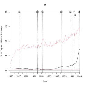
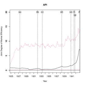
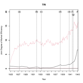
Figure 4: Time-Varying Degree of Market Efficiency (TSE New Shares)

Second, the Monthly Survey describes the positive factors produced by monetary easing, and the stock market was expected to rebound until the mid-1928. It also indicates that the negative factors related to lifting the ban increased, and the stock prices, especially TSE’s new shares, plummeted from April to May 1929, owing to the possibility of a changing exchange rate system. When this uncertainty reached its limit, the Hamaguchi Cabinet issued a statement in July 1929, announcing the implementation of the gold embargo (the return to the gold standard was implemented in January 1930). This announcement had made clear the outlook of market participants and the degree of market efficiency of TSE’s new shares to increase further, as depicted in Figure 4.

(Figure 4 around here)

Surprisingly, the Great Crash of October 1929 was not highlighted as a negative factor in the Monthly Survey, and the market participants believed that the subsequent softening of stock prices until November 1930 was not significantly affected by overseas markets. The focus on commodity markets and trade as negative factors indicates that fixing the exchange rate with the old exchange rate—which was stronger than before—caused a sharp decline in commodity markets and highlighted the concerns over the deterioration of the domestic economy due to increasing imports, particularly from China. The New York stock market’s collapse seriously affected the world economy, producing a turning point wherein governments restricted foreign trade to protect domestic industries. However, Japan had faced the Showa Financial Crisis in 1927, owing to which its stock market was in decline and the adverse effect of returning to the gold standard system worsened the situation. As the monthly average of the deferment fee of short-term clearing futures transactions fell below zero during mid-1930, the demand for short-selling and the fee of lending stocks increased.

When the sterling pound fell after the U.K. announced the suspension of the gold standard system in September 1931, the forecast around the abandonment of the system intensified in Japan. Therefore, stock buying, which expected a rebound in stock prices, accelerated toward the end of the year. The change in the exchange rate policy in Japan significantly altered market participants’ behaviours, along with a rapid increase of long positions. The deferment fee of TSE’s new shares increased to 190 sen ($=1.90$ yen) in December 1931, which was the highest in history for short-term clearing futures transactions. As described above, the period of extreme increases in short positions in the stock market was followed by a period of significant increases in long positions, and the market efficiency generally continued to decline during the gold ban period.

Third, the degree of market efficiency based on the EQPI and TSE’s new shares declined and then bottomed out in December 1931 with the ban on gold exports (turning point (b) in Table 6). This policy change cleared the fog of uncertainty about the future and increased confidence in the prospects of market participants. In December 1931, Korekiyo Takahashi became the Minister of Finance, and decided to withdraw from the gold standard system. This caused the rapid appreciation of the U.S. dollar against the yen and an uptrend in the stock market. In July 1932, the Capital Flight Prevention Law was enacted, but did not prevent the decline of the exchange rate directly. Therefore, the yen continued to depreciate against the U.S. dollar until November 1932, when the Ministry of Finance’s ordinance was announced. According to Fukai (1941), the Capital Flight Prevention Law did not restrict the freedom of transactions as much as possible, but left it to the self-restraint of exchange market participants.

The Monthly Survey reports that, while overseas politics became a negative factor, owing to the growing international criticism of the Manchurian incident, the stock market was affected by positive factors as well, such as the low exchange rate caused by the rapid depreciation of the yen, and by domestic finance and bonds, such as the underwriting of Japanese government bonds by the Bank of Japan.

In November 1932, the ordinance of the Ministry of Finance required each foreign exchange bank to report the contents of their foreign exchange transactions promptly. It became evident that the Japanese government’s stance on exchange rates had shifted from a policy of laissez faire to preventing a decline in exchange rates. The Foreign Exchange Control Law was promulgated in March 1933 and enforced in May 1933 (turning point (c) in Table 6). Uncertainty about the prospect of a major policy shift, ending the gold standard, has been resolved, stock markets have priced in the change, and stock markets have become more efficient. The elimination of uncertainty over the international financial system, as it were, also signaled the beginning of uncertainty in international relations, and the efficiency of the stock market peaked in the spring of 1933.

6.2 Withdrawal of the U.S. Gold Standard and Strengthening of Control over the Japanese Economy (April 1933–August 1945)

In April 1933, U.S. President Franklin D. Roosevelt announced the abolishment of the gold standard. This reversed the yen’s depreciation in 1932 and instigated the U.S, dollars depreciation in 1933. And after that the U.S. dollar and the pound remained stable against the yen until the beginning of WWII. From then on, the degree of market efficiency bottomed out and trended downward until the mid of WWII.

First, the trading ratio of long-term clearing futures transactions increased, owing to the broad trading of shares excluding TSE. There was no significant change in the deferment fee. This suggests that trading was not conducted in an extraordinary market environment with trading being biased in one direction (see Figures 1 and 2). Thereafter, according to the Monthly Survey, corporate performance affected the stock market in 10 out of 48 cases in 1934 and 24 out of 58 cases in 1935. While market participants recognised these items as a positive factor in 1934 owing to an increase in profits and dividends, they were perceived as a negative factor in 1935 because of a decrease in dividends. At the end of 1935, stocks were selected based on business performance, which corresponds with a selective market that considered the merits and demerits of businesses and companies.

The 26 February incident in 1936 ended Takahashi’s economic policy. As military spending increased and government bonds were issued in large quantities, the control of the government bond market was strengthened and government intervention in the market increased significantly. Since the end of Takahashi’s policy, market efficiency had declined further amid the shift to a wartime regime and increased government intervention in financial markets. After 1937, the stock market became less volatile and the deferment fee for short-term clearing futures transactions stabilised, except for 1940 and 1941. In particular, the stock market became more dependent on the domestic political situation than the overseas economic environment. The Monthly Survey has suggested that the influences of the international political situation and domestic policy on stock price fluctuation have increased since 1936. In addition to the deterioration of international relations with China and the Soviet Union, domestic policy conditions, such as stricter controls and higher taxes, became negative factors. Simultaneously, international conflicts in Europe and domestic policy issues, such as the establishment of stock price-keeping institutions and fiscal expansion, became positive factors for stock prices.

Although the TSE trading volume reached a prewar high in March 1937, the Second Sino-Japanese War broke out in July, and the value of the EQPI swung back and forth until 1939. The Monthly Survey includes several descriptions of domestic policies and international politics. For the former, stock price-keeping operations (market intervention) by Dainippon Shoken Toshi and Seiho Shoken (stock prices keeping institutions) worked as a positive factor, while tighter controls, such as the restriction of stock dividends by invoking Article 11 of the National Mobilization Law and the National Electricity Management Law, worked as negative factors. From then until the end of 1940, market efficiency remained on slightly improving trend (turning point (d) in Table 6). For the latter, the outbreak of the Second Sino-Japanese War and concerns over its duration worked as negative factors and the improvement of the war situation, such as the fall of Nanjing, worked as a positive factor (see Table 5).

Second, in September 1939, with expectations of an early end of the Second Sino- Japanese War and the declaration of war by the U.K. and France against Germany, the profits of export-related companies were predicted to expand and stock prices rose as a result. Meanwhile, the degree of market efficiency based on the EQPI increased a little after the outbreak of the European War (see Figure 3).

In September 1940, the Tripartite Pact between Japan, Germany and Italy was signed, the stock price of TSE’s new shares had fallen more than 14% in a month. Subsequently, in December 1940, the Japanese government announced an Outline of the New Economic Order (turning point (e) in Table 6). This outline curtailed the rights of shareholders and accelerated the transfer of decision-making power to corporate managers and employees for the supply of wartime supplies. The prospects of stock market participants were confused, and the function of reacting all kinds of information to stock prices was paralyzed. From then until July 1941, Japanese government intervention in the stock market became more extreme and the degree of the market efficiency plummeted (turning point (f) in Table 6). Nippon Shoken Toshi (one of the stock prices keeping institutions) was established to stabilise stock prices and, in March 1941, Nippon Kyodo Shoken (the other stock prices keeping institution) was established to bolster them. In July 1941, stock prices fell sharply because of U.S.’s freeze on the assets held by Japan. Consequently, deferment fees dropped sharply and TSE’s new shares recorded the lowest price of 300 sen ($=3$ yen), while the lowest average of all short-term clearing futures transactions was 163 sen ($=1.63$ yen). Therefore, the asset freezing significantly affected the Japanese stock market, causing a rapid increase in short positions. During this period, the government issued a loan order to the Industrial Bank of Japan to supply money to increase stock prices. In August 1941, the Stock Price Control Ordinance was promulgated and enacted, which allowed the government to limit the minimum stock price. At this juncture, the peace negotiations seemed to have progressed, so market efficiency improved temporarily, cushioning the shock of the asset freeze. However, with the resignation of the Konoe Cabinet and the formation of the Tojo Cabinet, “war risk premium” was imposed and market efficiency deteriorated again (turning point (g) in Table 6).

Third, when the Pacific War broke out after Japan attacked Pearl Harbor in December 1941, stock prices, particularly TSE’s new shares, increased significantly. The government intervened to restrain prices (selling intervention) because market volatility increased in response to the rising expectations of victory. Nippon Kyodo Shoken continued selling between mid-December 1941 and January 1942, as the rise in stock prices did not decline. The Stock Price Control Ordinance was revised to allow the establishment of maximum stock prices and the Ministry of Finance imposed a capital gain tax (tax on trading profits of liquidation transactions) to restrain overheating transactions. Unlike the government bond market, wherein the yield level was almost fixed, this market intervention was implemented to deal with excessive fluctuations because of price elasticity in the stock market. In April 1942, Nippon Kyodo Shoken was absorbed by the powerful Wartime Finance Bank, and the conventional stock price-keeping policy changed to a stock price-stabilisation policy after the outbreak of the war against the U.S.

After the Battle of Midway, the government attempted to restrain the rise in stock prices. When the stock market began to weaken, the government intervened actively to protect stock prices. In other words, during the war, the government implemented policies to control market volatility by preventing excessive increases and decreases of stock prices. After the Pacific War broke out in December 1941 (until June 1943), the deferment fee remained stable, and there was little need for the agencies to intentionally manipulate it. Moreover, the market efficiency improved at a time when many hoped they had a better chance of winning the war early. Many of the early battles, such as the Battle of Midway, were reported in the Japanese media with overestimation of the results of the war, but after the fall of Guadalcanal in early 1943, it became impossible to hide the deterioration of the war situation. And as the diluted war risk premium was re-realized, market efficiency deteriorated again (turning point (h) in Table 6). After 1943, market efficiency showed signs of deteriorating again, but in the year following the outbreak of the Pacific War, market efficiency improved rapidly. It seems that this is inconsistent with Suzuki (2012) who concluded that market efficiency deteriorated after the start of the Pacific War. However, as Figure 4 shows, the same results as Suzuki (2012) are obtained when new TSE shares are used as stock returns.

On the other hand, in December 1942, the government decided TSE’s shares were delisted from the stock exchanges and various exchanges were reorganised into the Japan Stock Exchange in August 1943. As a result, the deferment fee of TSE’s new shares fell significantly. During this period, the trading ratio of short-term clearing futures transactions in the TSE declined significantly, while those of long-term clearing futures transactions and spot transactions increased. This reflected the rapid development during this period. The degree of market efficiency of TSE’s new shares resulted in a sharp decline from sell-off to delisting. While the stock market experienced a sharp recovery in the market efficiency until early 1943, the efficiency of TSE’s new shares deteriorated rapidly from the beginning of 1942. As control of the exchange shifted from the Ministry of Commerce and Industry to the Ministry of Finance in December 1941, the prospect of delisting of the TSE increased, and efficiency probably declined sharply over the year leading up to the announcement (see Figure 4). The market capitalization weight of TSE’s new shares was less than 2% according to the EQPI; hence, the effect of the degree of market efficiency on the EQPI was not significant.

6.3 Summary of Changes in the Degree of Market Efficiency in the Early Showa Period

Contrary to Bassino and Lagoarde-Segot (2015), we find that the stock market was almost efficient throughout the sample period. The differences in the results are attributed to differences in the datasets and the verification methods. Their sample period extends from January 1931 to December 1940, while our sample period covers June 1924 to June 1943, including the period when price controls were tightened at the end of the war. Bassino and Lagoarde-Segot (2015) do not include the period of WWII, when volatility was controlled by the Stock Price Control Ordinance and, thus, examine the efficiency during periods of relatively high volatility. Clearly, market efficiency tends to decline during periods of high volatility. The fact that Bassino and Lagoarde-Segot (2015) use the time-invariant GARCH-in-mean model as the verification method also explains the difference from our results.

As Hoshi and Kashyap (2001) point out, the proportion of Japanese companies that raised money through the stock market declined during the war, and this amount may have been low. However, a certain level of market efficiency might have been maintained over time, due to the existence of clearing transactions that were not affected by the flow of funds. Hirayama (2020) also confirms the price elasticity of major stocks (Nippon Yusen Kaisha and Kanegafuchi Industries) in spot transactions even in 1945, when financial controls were further tightened after the period covered by this study.

Price controls in financial markets worked strongly for government bonds, but had relatively little impact on equity markets, which only prevented them from over-rising and falling sharply. Market efficiency during the war years was worse than in the early 1930s due to government intervention, but it did not reach the level of inefficiency. This conclusion suggests that the peculiarities of the prewar Japanese stock market affected the efficiency evaluation by selecting the stock indices to be tested.

7 Concluding Remarks

This study investigates the relationships between major historical events and the efficiency of the prewar Japanese stock market in the context of the AMH. In particular, we estimate the degree of market efficiency in the prewar Japanese stock market using Ito et al.’s (2014; 2016; 2022) GLS-based time-varying parameter model, and employ primary historical documents to clarify the factors that caused efficiency to fluctuate over time from a historical perspective.

Our empirical results can be summarised as follows. First, the degree of market efficiency in the prewar Japanese stock market varied over time, corresponding to major historical events. Second, our results show that the AMH is supported in this market, in line with Noda (2016), who tested the AMH for the post-WWII Japanese stock market. Third, the study concludes that market efficiency was maintained throughout the period (from June 1924 to June 1943). The variation in market efficiency observed in this study differs significantly from that in previous studies, such as Kataoka et al. (2004) and Bassino and Lagoarde-Segot (2015). We find that this difference depends on whether the price index is capitalisation-weighted. Finally, stronger price controls since the mid-1930s and wartime market intervention by stock price maintenance agencies restrained price volatility. As the Japanese government intervention in the market intensified throughout the 1930s, the market efficiency declined, as well as rapidly taking into account the war risk premium, especially from the time when the Pacific War became inevitable.

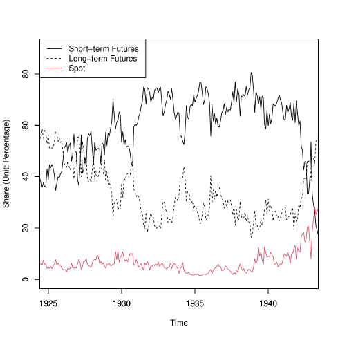
Figure 1: Trading Volume Share on the Market by Type of Transaction

Source: Tokyo Stock Exchange (1938) and The Monthly Statistical Report of Tokyo Stock Exchange, June 1924–June 1943.

Table 1: Factors Affecting Stock Prices Based on the Bank of Japan’s Monthly Survey

		1924	1925	1926	1927	1928	1929	1930	1931	1932	1933	1934	1935	1936	1937	1938	1939	1940	1941	Total
Domestic	Political Events	1	2	2	2	7	8	3	3	5	6	8	3	3	7	3	1	1	1	66
	Policy Matters	4	2	5	3	6	8	9	2	9	7	9	4	18	18	17	12	16	5	154
	Financial Markets	2	9	9	18	8	3	1	8	14	10	5	1	4	10	3	6	4	1	116
	Bond Markets	$-$	1	$-$	1	4	2	1	7	3	3	2	$-$	1	2	$-$	$-$	$-$	$-$	27
	Commodity Markets	5	7	11	5	8	3	11	2	9	6	2	7	4	8	4	4	$-$	1	97
	Foreign Exchange	$-$	1	4	3	1	7	1	4	11	12	2	2	2	1	$-$	$-$	$-$	$-$	51
	Trade Status	2	2	6	6	1	$-$	11	8	5	4	2	3	5	4	7	$-$	2	2	70
	Corporate Performance	3	11	7	8	6	5	7	6	9	7	10	24	17	5	8	7	4	$-$	144
Overseas	Political Events	1	3		5	3	5	3	4	18	24	6	9	10	17	16	14	21	11	170
	Economic Situation	3	$-$	1	1	$-$	1	$-$	3	5	4	1	4	1	1	3	$-$	$-$	$-$	28
	Financial Markets	$-$	3	1	$-$	$-$	$-$	2	2	1	3	$-$	$-$	$-$	$-$	$-$	$-$	$-$	$-$	12
	Commodity Markets	1	$-$	2	$-$	$-$	$-$	1	8	1	5	1	1	$-$	3	$-$	$-$	$-$	$-$	23
	Stock Markets	0	4	5	0	1	0	0	7	4	4	0	0	0	3	2	1	0	0	31
Total		22	45	53	52	45	42	50	64	94	95	48	58	65	79	63	45	48	21	989

Source: Bank of Japan, Research Department, Monthly Survey (June 1924–April 1941).

Source: As for Figure 1.

Table 2: Characteristics of Price Indexes in the Prewar Japanese Stock Market

Database	Type of Average Index	Sample Period	Frequency	Adjusted Index	Total Index
Toyo Keizai Shimpo	Simple Arithmetic Average	1916/01-44/05	Monthly	No	No
Toyo Keizai Shimpo	Simple Arithmetic Average	1930/06-40/12	Daily	No	No
Bank of Japan	Simple Arithmetic Average	1924/01-42/06	Monthly	No	No
Tokyo Stock Exchange	Volume-weighted	1921/01-45/08	Monthly	No	No
Nippon Kangyo Bank	Simple Arithmetic Average	1910/12-45/01	Monthly	No	No
EQPI (Hirayama (2018, 2020))	Capitalization-weighted	1924/06-45/08	Monthly	Yes	Yes

Notes:

• This table relies heavily on Hirayama (2018).

• “Adjusted Index” denotes the modified price index in the case of ex-rights and additional paid-in capital.

• “Total Index” denotes the modified price index, which additionally accounts for the dividend.

Table 3: Descriptive Statistics and Unit Root Tests

		$R_{PI}$	$R_{API}$	$R_{TRI}$	$C_{DEF}$
Mean		0.0005	0.0009	0.0055	$-0.0009$
SD		0.0481	0.0474	0.0480	0.4009
Min		$-0.1633$	$-0.1633$	$-0.1580$	$-3.5419$
Max		0.1991	0.1991	0.1991	3.4484
ADF-GLS		$-10.2868$	$-10.2559$	$-10.7104$	$-15.1517$
Lags		0	0	0	1
$\hat{\phi}$		0.3622	0.3648	0.3266	$-0.2952$
$\mathcal{N}$		228

Notes:

• “$R_{PI}$,” “$R_{API}$,” and “$R_{TRI}$” denote the returns on the price index, adjusted price index, and total return index, respectively.

• “$C_{DEF}$” denotes the chages in deferment fees.

• “ADF-GLS” denotes the ADF-GLS test statistics, “Lags” denotes the lag order selected by the MBIC, and “$\hat{\phi}$” denotes the coefficient vector in the GLS detrended series; see Equation (6) in Ng and Perron (2001).

• In the ADF-GLS test, a model with a time trend and a constant is assumed. The critical value at the 1% significance level for the ADF-GLS test is “$-3.42$.”

• “$\mathcal{N}$” denotes the number of observations.

• R version 4.2.2 is used to compute the statistics.

Table 4: Preliminary Estimations and Parameter Constancy Tests

		$R_{PI,t}$	$C_{DEF,t}$		$R_{API,t}$	$C_{DEF,t}$		$R_{TRI,t}$	$C_{DEF,t}$
$Constant$		0.0001	$-0.0029$		0.0004	$-0.0030$		0.0044	$-0.0039$
		[0.0032]	[0.0200]		[0.0031]	[0.0202]		[0.0033]	[0.0217]
$R_{i,t-1}$		0.3463	1.6212		0.3431	1.5942		0.3067	1.5531
		[0.0462]	[0.6345]		[0.0440]	[0.6414]		[0.0477]	[0.6686]
$C_{DEF,t-1}$		0.0004	$-0.4743$		0.0003	$-0.4726$		0.0007	$-0.4742$
		[0.0079]	[0.1060]		[0.0078]	[0.1063]		[0.0079]	[0.1069]
$R_{i,t-2}$		$-0.1619$	$-1.2968$		$-0.1760$	$-1.3005$		$-0.1515$	$-1.3392$
		[0.0733]	[0.3996]		[0.0733]	[0.4090]		[0.0804]	[0.3972]
$C_{DEF,t-2}$		$-0.0028$	$-0.2659$		$-0.0005$	$-0.2637$		$-0.0018$	$-0.2592$
		[0.0079]	[0.1007]		[0.0087]	[0.1006]		[0.0083]	[0.0993]
$\bar{R}^{2}$		0.0987	0.1922		0.0983	0.1903		0.0779	0.1921
$L_{C}$		23.0428			22.5818			22.6711

Notes:

• “$R_{i,t-p}$” and “$C_{DEF,t-p}$” denote the VAR($p$) estimate for each return and chages in deferment fees.

• “$\bar{R}^{2}$” and “$L_{C}$” denote adjusted $R^{2}$ and Hansen’s (1992) joint $L$ statistic with variance.

• Newey and West’s (1987) robust standard errors are given in brackets.

• R version 4.2.2 is used to compute the estimates.

Table 5: Major Historical Events in Prewar Japan

	Period		Major historical event
	Apr 1925		The Bank of Japan reduced the official discount rate to 7.30%.
	Oct 1926		The Bank of Japan reduced the official discount rate to 6.57%.
	Apr 1927		Nationwide financial panic sparked when debates in the Diet revealed financial difficulties between the Bank of Taiwan and Suzuki & Co. (Showa Financial Crisis).
	Apr–May 1927		The Japanese government declared a moratorium on payments (bank holidays) on 22 April to last until 13 May.
	Jul 1929		The Hamaguchi Cabinet (Junnosuke Inoue was appointed the Minister of Finance) announced that the gold embargo would be lifted.
	Oct 1929		The Great Crash occurred.
	Jan 1930		The Japanese government lifted the gold embargo.
	Oct 1930		The SEIHO SHOKEN (life insurance companies) started stock price-keeping operations.
	Sep 1931		The United Kingdom abandoned the gold standard.
	Dec 1931		The Inukai Cabinet (Korekiyo Takahashi was appointed the Minister of Finance) abandoned the gold standard.
	Nov 1932		The announcement of the Ordinance of the Ministry of Finance clarified that the government’s policy was to prevent the yen from falling. The Bank of Japan started underwriting government bonds.
	Feb 1933		The prospect of Japan withdrawing from the League of Nations emerged.
	Mar 1933		The Foreign Exchange Control Law was promulgated.
	Apr 1933		The United States announced its abandonment of the gold standard.
	Feb 1936		The February 26 incident occurred; Korekiyo Takahashi’s economic policy ended.
	Mar 1937		The Tokyo Stock Exchange recorded the highest trading volume in the prewar period.
	Jul 1937		The Second Sino–Japanese War occurred.
	Apr 1938		The National Mobilization Law was promulgated and enforced.
	Sep 1939		World War II broke out.
	Jul 1941		President Franklin Roosevelt froze all Japanese assets in the United States.
	Aug 1941		The Stock Price Control Ordinance was promulgated and enforced.
	Dec 1941		The Pacific War broke out.
	Jun 1942		The Battle of Midway broke out.
	Dec 1942		The Japanese government decided to delist Tokyo Stock Exchange shares.
	Aug 1943		The Tokyo Stock Exchange delisted short-term clearing futures transactions.
	Jul 1944		Operation Forager (the Battle of Saipan) ended. The Wartime Finance Bank started stock price-keeping operations.
	Mar 1945		The Great Tokyo Air Raids occurred; the Wartime Finance Bank started stock price-keeping operations (unlimited stock purchases). In July, the Japan Stock Exchange started stock price-keeping operations.
	Aug 1945		The Pacific War ended.

Note: This table is mainly constructed following Institute for Monetary and Economic Studies, Bank of Japan (1993).

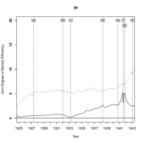
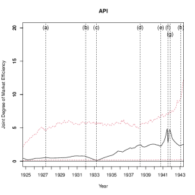
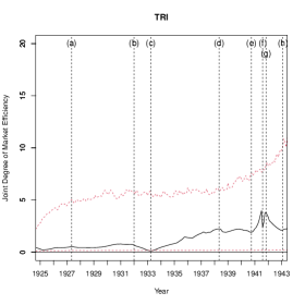
Figure 3: Time-Varying Degree of Market Efficiency (EQPI)

Notes:

• The points (a)–(h) in the figure are consistent with the time periods in Table 6.

• The dashed red lines represent 99% confidence intervals of the efficient market degrees.

• We run the bootstrap sampling 10,000 times to calculate the confidence intervals.

• R version 4.2.2 is used to compute the estimates.

Table 6: Turning Points in the Prewar Japanese Stock Market from the Viewpoint of Market Efficiency

	Period	Degree of market efficiency	Major historical event
	(a) Apr–May 1927	Bottom Out	Nationwide financial panic sparked (Showa Financial Crisis).
			The Japanese government declared a moratorium on payments.
	(b) Dec 1931	Start of the Rise	The Inukai Cabinet abandoned the gold standard.
	(c) Mar–Apr 1933	Peak Out	Japan withdrew from the League of Nations.
			The Foreign Exchange Control Law was promulgated.
			The U.S. announced its abandonment of the gold standard.
	(d) Apr–May 1938	Bottom Out	The National Mobilization Law was promulgated and enforced.
	(e) Sep–Dec 1940	Peak Out	The Tripartite Pact between Japan, Germany and Italy was signed.
			The Japanese government announced an Outline of the New Economic Order.
	(f) Jul–Aug 1941	Double Bottom (1)	President Franklin Roosevelt froze all Japanese assets in the U.S.
			The Stock Price Control Ordinance was promulgated and enforced.
	(g) Oct–Dec 1941	Double Bottom (2)	The third Konoe Cabinet resigned en masse and the Tojo Cabinet was established.
			The Pacific War broke out.
	(h) Jan–Feb 1943	Peak Out	The Japanese forces began to withdraw from Guadalcanal.

Note: As for Figure 3.

References

- Bank of Japan (1948) Bank of Japan (1948), “Manshu Jihen Igo no Zaisei Kinyushi [Fiscal and Financial History after the Manchurian Incident],” Tokyo, Japan.
- Barro (2006) Barro, R. J. (2006), “Rare Disasters and Asset Markets in the Twentieth Century,” QuarterJournal of Economics, 121, 823–866.
- Bassino and Lagoarde-Segot (2015) Bassino, J. and Lagoarde-Segot, T. (2015), “Informational Efficiency in the Tokyo Stock Exchange, 1931–40,” Economic History Review, 68, 1226–1249.
- Berkman et al. (2011) Berkman, H., Jacobsen, B., and Lee, J. (2011), “Time-Varying Rare Disaster Risk and Stock Returns,” Journal of Financial Economics, 101, 313–332.
- Caldara and Iacoviello (2022) Caldara, D. and Iacoviello, M. (2022), “Measuring Geopolitical Risk,” American Economic Review, 112, 1194–1225.
- Choi (1999) Choi, I. (1999), “Testing the Random Walk Hypothesis for Real Exchange Rates,” Journal of Applied Econometrics, 14, 293–308.
- Choudhry (2010) Choudhry, T. (2010), “World War II Events and the Dow Jones Industrial Index,” Journal of Banking and Finance, 34, 1022–1031.
- Elliott et al. (1996) Elliott, G., Rothenberg, T. J., and Stock, J. H. (1996), “Efficient Tests for an Autoregressive Unit Root,” Econometrica, 64, 813–836.
- Engle et al. (1987) Engle, R., Lilien, D., and Robins, R. (1987), “Estimating Time Varying Risk Premia in the Term Structure: The ARCH-M Model,” Econometrica, 55, 391–407.
- Escanciano and Lobato (2009) Escanciano, C. and Lobato, I. (2009), “An Automatic Portmanteau Test for Serial Correlation,” Journal of Econometrics, 151, 140–149.
- Escanciano and Velasco (2006) Escanciano, C. and Velasco, C. (2006), “Generalized Spectral Tests for the Martingale Difference Hypothesis,” Journal of Econometrics, 134, 151–185.
- Fama (1970) Fama, E. F. (1970), “Efficient Capital Markets: A Review of Theory and Empirical Work,” Journal of Finance, 25, 383–417.
- Federation of Economic Research Institutes (1943) Federation of Economic Research Institutes (1943), Nihon Keizai Nenshi [Annual Report on the Japanese Economy], Senshin Sha, Tokyo, Japan.
- Fisher (1921) Fisher, I. (1921), “The Best Form of Index Number,” Quarterly Publications of the American Statistical Association, 17, 533–537.
- Fujino and Akiyama (1977) Fujino, S. and Akiyama, R. (1977), Shoken to Rishiritsu: 1874–1975 [Securities and Interest Rates: 1874–1975], Hitotsubashi University Economic Research Institute, Japan Economic Statistics Literature Center.
- Fukai (1941) Fukai, E. (1941), Kaiko 70-nen [Reflections of 70 Years], Iwanami Shoten, Tokyo.
- Hamao et al. (2009) Hamao, Y., Hoshi, T., and Okazaki, T. (2009), “Listing Policy and Development of the Tokyo Stock Exchange in the Prewar Period,” in Financial Sector Development in the Pacific Rim, East Asia Seminar on Economics, eds. Ito, T. and Rose, A., University of Chicago Press, vol. 18, pp. 51–87.
- Hansen (1992) Hansen, B. E. (1992), “Testing for Parameter Instability in Linear Models,” Journal of Policy Modeling, 14, 517–533.
- Hirayama (2018) Hirayama, K. (2018), “The Japanese Equity Performance Index in the Early Showa Era (in Japanese),” Journal of Financial and Securities Markets (Japan Securities Research Institute), 101, 71–91.
- Hirayama (2020) — (2020), “The Japanese Equity Performance from 1944 to 1945 (in Japanese),” Journal of Financial and Securities Markets (Japan Securities Research Institute), 109, 63–85.
- Hirayama (2021) — (2021), “The Japanese Government Bond Performance from 1944 to 1945 (in Japanese),” Journal of Financial and Securities Markets (Japan Securities Research Institute), 113, 1–27.
- Hirayama (2022) — (2022), “Stock Market Functions and Short-term Clearing Transactions in the Prewar Period (in Japanese),” Journal of Financial and Securities Markets (Japan Securities Research Institute), 117, 77–98.
- Hoshi and Kashyap (2001) Hoshi, T. and Kashyap, A. (2001), Corporate Finance and Governance in Japan: The Road to the Future, MIT Press.
- Institute for Monetary and Economic Studies, Bank of Japan (1993) Institute for Monetary and Economic Studies, Bank of Japan (1993), “Chronology of Financial Matters in Japan (in Japanese),” Institute for Monetary and Economic Studies, Bank of Japan, revised Edition.
- Ito et al. (2014) Ito, M., Noda, A., and Wada, T. (2014), “International Stock Market Efficiency: A Non-Bayesian Time-Varying Model Approach,” Applied Economics, 46, 2744–2754.
- Ito et al. (2016) — (2016), “The Evolution of Stock Market Efficiency in the US: A Non-Bayesian Time-Varying Model Approach,” Applied Economics, 48, 621–635.
- Ito et al. (2022) — (2022), “An Alternative Estimation Method for Time-Varying Parameter Models,” Econometrics, 10, 23.
- Ito and Sugiyama (2009) Ito, M. and Sugiyama, S. (2009), “Measuring the Degree of Time Varying Market Inefficiency,” Economics Letters, 103, 62–64.
- Kataoka et al. (2004) Kataoka, Y., Maru, J., and Teranishi, J. (2004), “An Analysis of Stock Market Efficiency in the Late Meiji Era, Part.2 (in Japanese),” Journal of Financial and Securities Markets (Japan Securities Research Institute), 48, 69–81.
- Kim et al. (2011) Kim, J. H., Shamsuddin, A., and Lim, K. P. (2011), “Stock Return Predictability and the Adaptive Markets Hypothesis: Evidence from Century-Long U.S. Data,” Journal of Empirical Finance, 18, 868–879.
- Lim and Brooks (2011) Lim, K. P. and Brooks, R. (2011), “The Evolution of Stock Market Efficiency Over Time: A Survey of the Empirical Literature,” Journal of Economic Surveys, 25, 69–108.
- Lim et al. (2013) Lim, K. P., Luo, W., and Kim, J. H. (2013), “Are US Stock Index Returns Predictable? Evidence from Automatic Autocorrelation-Based Tests,” Applied Economics, 45, 953–962.
- Lo (2004) Lo, A. W. (2004), “The Adaptive Markets Hypothesis: Market Efficiency from an Evolutionary Perspective,” Journal of Portfolio Management, 30, 15–29.
- Lo (2005) — (2005), “Reconciling Efficient Markets with Behavioral Finance: The Adaptive Markets Hypothesis,” Journal of Investment Consulting, 7, 21–44.
- Malkiel (2004) Malkiel, B. G. (2004), A Random Walk Down Wall Street: The Time-Tested Strategy for Successful Investing, W. W. Norton & Company, Inc.
- Newey and West (1987) Newey, W. K. and West, K. D. (1987), “A Simple, Positive Semi-Definite, Heteroskedasticity and Autocorrelation Consistent Covariance Matrix,” Econometrica, 55, 703–708.
- Ng and Perron (2001) Ng, S. and Perron, P. (2001), “Lag Length Selection and the Construction of Unit Root Tests with Good Size and Power,” Econometrica, 69, 1519–1554.
- Noda (2016) Noda, A. (2016), “A Test of the Adaptive Market Hypothesis using a Time-Varying AR Model in Japan,” Finance Research Letters, 17, 66–71.
- Okazaki (1999) Okazaki, T. (1999), “Corporate Governance,” in The Japanese Economic System and its Historical Origins, eds. Okuno-Fujiwara, M. and Okazaki, T., Oxford University Press.
- Perron (1997) Perron, P. (1997), “Further Evidence on Breaking Trend Functions in Macroeconomic Variables,” Journal of Econometrics, 80, 355–385.
- Reitz (1988) Reitz, T. A. (1988), “The Equity Risk Premium: A Solution,” Journal of Monetary Economics, 22, 117–131.
- Schwarz (1978) Schwarz, G. (1978), “Estimating the Dimension of a Model,” Annals of Statistics, 6, 461–464.
- Shibata (2011) Shibata, Y. (2011), Senji Nihon no Kinyu Tosei [Monetary Controls in Wartime Japan], Nihon Keizai Hyoron Sha, Tokyo.
- Shiller (2005) Shiller, R. J. (2005), Irrational Exuberance: Second Edition, Princeton University Press.
- Suzuki (2012) Suzuki, S. (2012), “Pacific War and Tokyo Stock Exchange Daily Data:1941-1943 (in Japanese),” Bulletin of Economic Studies (Meisei University), 44, 39–51.
- Takahashi (1955) Takahashi, K. (1955), Taisho Showa Zaikai Hendoshi [Economic Trends during the Taisho and Showa Periods], vol. 2–3, Toyo Keizai Shimposha.
- Tokyo Stock Exchange (1938) Tokyo Stock Exchange (1938), History of the Tokyo Stock Exchange (in Japanese), vol. 3, Tokyo Stock Exchange.
- Verdickt (2020) Verdickt, G. (2020), “The Effect of War Risk on Managerial and Investor Behavior: Evidence from the Brussels Stock Exchange in the pre-1914 Era,” Journal of Economic History, 80, 629–669.