Control of accuracy on Taylor-collocation method for load leveling problem

Аннотация

High penetration of renewable energy sources coupled with decentralization of transport and heating loads in future power systems will result even more complex unit commitment problem solution using energy storage system scheduling for efficient load leveling. This paper employees an adaptive approach to load leveling problem using the Volterra integral dynamical models. The problem is formulated as solution of the Volterra integral equation of the first kind which is attacked using Taylor-collocation numerical method which has the second-order accuracy and enjoys self-regularization properties, which is associated with confidence levels of system demand. Also the CESTAC method is applied to find the optimal approximation, optimal error and optimal step of collocation method. This adaptive approach is suitable for energy storage optimization in real time. The efficiency of the proposed methodology is demonstrated on the Single Electricity Market of the Island of Ireland.

51-74 45D05, 65D30

1 Introduction

Robust numerical methods design for optimized energy storage and load leveling is one of the most imminent challenges in power systems. The conventional least-cost dispatch of available generation to meet the forecasted load will no longer be suitable for the purposes because of observed decentralization of power systems including electrical transport and heating loads and renewable energy use worldwide. Various methods have been examined to solve this challenging problem including the evolutionary methods, and genetic algorithms, Lagrangian relaxation, mixed integer linear programming and particle swarm optimization. The transmission system operator in Republic of Ireland restricts the instantaneous proportion of total generation allowed from wind wind turbines, to 50 % maximum, in order to maintain sufficient system inertia [29]. This may result in wind curtailment at any time. The reduction of the uncertainty associated with wind power can be achieved using the state of the art forecasting methods based on contemporary machine learning theory. Wind power and industrial and residential electric load forecasting, over lead times of up to 48 hours, are critical for the market operator. These forecasts are used to create day-ahead unit commitment and economic dispatch schedules. In fact, many transmission system operators in Russia and in other countries also employ the shorter-term wind forecasts to draw upon system reserves for short-term balancing. It is to be noted here that a reduction in the forecast errors by a fraction of a percent will lead to a substantial increase in trading profits. The efficient forecast algorithms increase the value of wind generation. In [28] it is shown that an increase of only one percent in forecast error caused an increase of 10 million GBP in operating costs per year for one electric utility in the UK. For the detailed review of China coal-fired power units peak regulation with a detailed presentation of the installed capacity, load leveling operation mode readers may refer to [12]. The effectiveness of wind turbine, energy storage, and demand response programs in the deterministic and stochastic circumstances and influence of uncertainties of the wind, price, and demand are assessed in the Energy Hub planning in [19]. The unit commitment solver is supposed to serve as an integral part of Energy Hub for control of the interconnections of heterogeneous energy infrastructures, including non-synchronous renewable sources. This paper presents a methodology for load leveling using dynamical models based on efficient numerical solution of the integral equations (IE) of the first kind. We consider the future power systems with battery energy storages of various efficiencies. The load forecasts over lead times of 24 hours is used. The load leveling problem is formulated as inverse problem. These integral equations efficiently solve such an inverse problem given both the time-dependent efficiencies and the availability of generation/storage technologies. Electric load can be forecasted using various mathematical models including classical statistical methods of time series analysis, regressive models or advanced machine learning methods including deep learning. The evolutionary character of power systems when future values depend upon previous values can be described by evolutionary integral equations which are also known as Volterra equations. The integrand (or kernel) of employed equations has 1st kind discontinuities along the continuous curves starting at the origin. Such piecewise continuous kernels K(t,s) take into account both efficiencies of the different storing technologies and their proportions (which could be time-dependent) in the total power generation. Efficiencies of the different storages may depend not only on their age and use duration but also on the state of charge, see [32]. This phenomena can be modeled using the nonlinear Volterra integral equations.

In recent years many numerical or semi-analytical methods have been presented to solve the linear and non-linear first kind IEs [7, 8, 18, 26, 27, 30]. In this paper, we develop further the numerical methods for solution of such integral equations and continue our previous work [22] where we demonstrated how these novel models can be applied for storage modeling. In this work, the Taylor-collocation method [4, 6, 11, 20] is considered to solve the mentioned problem based on the stochastic arithmetic and the approximate results are validated by using the CESTAC method. Also, the optimal iteration and the optimal approximation of method are found. Recently, the CESTAC method has been applied to implement the numerical methods for finding the approximate solution of different problems [9, 10, 15, 16, 17]. In this method, instead of using the mathematical packages such as Matlab, Mathematica and the others, the CADNA library is applied. Also, in this library the logical programs can be written by statements of C/C++, FORTRAN or ADA [1, 2]. Some of the advantages of using the CESTAC method and CADNA library are:

• In the CESTAC method, not only the optimal numerical solution can be produced but also, the optimal iteration can be obtained [9, 10, 15, 17].

• The CADNA library is able to detect any instability in mathematical operations, branching, functions and so on but the FPA has not these abilities.

• In the FPA, the termination criterion depends on a small parameter like $h$ or epsilon. For epsilon enough large, the iterations can be stopped before finding the suitable approximation and for small values of epsilon the unnecessary iterations can be produced without improving the accuracy of the results [3, 31]. In the SA, the numerical results do not depend on the value epsilon and a new stopping condition is replaced which is independent of epsilon and existence of exact solution.

This paper is structured into four sections. The background on Volterra integral equations theory and numerical methods (including results on convergence) is described in Section 2. Section 3 describes the results of the numerical experiments on real data from the Irish test system. Section 4 draws a brief conclusion

2 Volterra model

The proposed collocation-type numerical method has the second-order accuracy and enjoys self-regularization properties as mesh step is associated with confidence levels of system demand. The proposed approach is suitable for energy storage control in real time.

Let us consider the first kind classical Volterra IE

$$\int_{0}^{t}K(t,s)x(s)ds=f(t),\leavevmode\nobreak\ 0\leq s\leq t\leq T,$$ (2.1)

where $K(t,s)$ is a discontinuous kernel along continuous curves $\alpha_{i},i=1,2,\cdots,m-1$ as

$$\left\{\begin{array}[]{l}K_{1}(t,s),\leavevmode\nobreak\ \leavevmode\nobreak\ \leavevmode\nobreak\ \leavevmode\nobreak\ \leavevmode\nobreak\ 0=\alpha_{0}(t)\leq s\leq\alpha_{1}(t),\\ \\ K_{2}(t,s),\leavevmode\nobreak\ \leavevmode\nobreak\ \leavevmode\nobreak\ \leavevmode\nobreak\ \leavevmode\nobreak\ \alpha_{1}(t)\leq s\leq\alpha_{2}(t),\\ \leavevmode\nobreak\ \leavevmode\nobreak\ \leavevmode\nobreak\ \vdots\\ K_{m}(t,s),\leavevmode\nobreak\ \leavevmode\nobreak\ \leavevmode\nobreak\ \leavevmode\nobreak\ \leavevmode\nobreak\ \alpha_{m-1}(t)\leq s\leq\alpha_{m}(t)=r\leq 1.\\ \end{array}\right.$$ (2.2)

Finally, Eq. (2.1) can be written in the following form

$$\int_{\alpha_{0}(t)}^{\alpha_{1}(t)}K_{1}(t,s)x(s)ds+\int_{\alpha_{1}(t)}^{\alpha_{2}(t)}K_{2}(t,s)x(s)ds+\cdots+$$

$$+\int_{\alpha_{m-1}(t)}^{\alpha_{m}(t)}K_{m}(t,s)x(s)ds=f(t),$$ (2.3)

where $f(0)=0$. Also, the compacted scheme of Eq. (2.3) is given as

$$\sum_{p=1}^{m}\int_{\alpha_{p-1}(t)}^{\alpha_{p}(t)}K_{p}(t,s)x(s)ds=f(t).$$ (2.4)

Recently, the IE with jump discontinuous kernel (2.4) have been solved by many mathematical methods [5, 13, 14, 21, 22, 23, 24, 25] based on the floating point arithmetic. In these researches and many other articles, the validation of presented methods are investigated by using the absolute error. But does this tool is a proper instrument to validate the numerical results? In many researches we can find the dependence of obtained results to the exact solution as

$$\left|x(s)-x_{n}(s)\right|\leq\varepsilon.$$ (2.5)

It means that without having the exact solution we can not study the accuracy of methods. Also, how are we sure about optimal value for number of iteration $n$? On the other hand, how can we apply the condition (2.5) without knowing the proper value of $\varepsilon$.

In this study, in order to solve the mentioned problems which are based on the FPA, the Taylor-collocation method based on the stochastic arithmetic is applied and then the obtained results are validated by using the CESTAC method and the CADNA library. Moreover, a novel stopping condition

$$\left|x_{n+1}(s)-x_{n}(s)\right|=@.0,$$ (2.6)

is presented instead of criterion (2.5) that it depends on two successive approximations. New algorithm will be stopped when difference of two successive approximations equals to informatical zero $@.0$. Let

$$x_{n}(s)=\sum_{j=0}^{n}\frac{1}{j!}x^{(j)}(c)(s-c)^{j}+O(h^{n+1}),$$ (2.7)

be the $n$-th order of Taylor polynomial at point $s=c$ where

$$e_{n}(s)=|x(s)-x_{n}(s)|=O(h^{n+1}).$$ (2.8)

By putting Eq. (2.7) into Eq. (2.4) we get

$$\sum_{p=1}^{m}\int_{\alpha_{p-1}(t)}^{\alpha_{p}(t)}K_{p}(t,s)\sum_{j=0}^{n}\frac{1}{j!}x^{(j)}(c)(s-c)^{j}ds=f(t).$$ (2.9)

Now, the collocation points

$$r_{i}=a+(\frac{b-a}{n})i,\leavevmode\nobreak\ \leavevmode\nobreak\ \leavevmode\nobreak\ \leavevmode\nobreak\ \leavevmode\nobreak\ i=0,1,\cdots,n,$$ (2.10)

should be substituted in Eq. (2.9) as follows

$$\sum_{j=0}^{n}\frac{1}{j!}\left[\sum_{p=1}^{m}\int_{\alpha_{p-1}(r_{i})}^{\alpha_{p}(r_{i})}k_{p}(r_{i},s)(s-c)^{j}ds\right]x^{(j)}(c)=f(r_{i}).$$ (2.11)

The matrix form of Eq. (2.11) is presented as

$$AV=F,$$ (2.12)

where

$$A=\left[\begin{array}[]{cccc}A_{00}&A_{01}&\cdots&A_{0n}\\ A_{10}&A_{11}&\cdots&A_{1n}\\ \vdots&\vdots&\ddots&\vdots\\ A_{n0}&A_{n1}&\cdots&A_{nn}\end{array}\right]_{(n+1)(n+1)},$$

that

$$A_{ij}=\sum_{p=1}^{m}\int_{\alpha_{p-1}(r_{i})}^{\alpha_{p}(r_{i})}k_{p}(r_{i},s)(s-c)^{j}ds,$$

and

$$V=\left[\begin{array}[]{cccc}\bar{x}^{(0)}(c)&\bar{x}^{(1)}(c)&\cdots&\bar{x}^{(n)}(c)\end{array}\right]^{T},$$

$$F=\left[\begin{array}[]{cccc}F(r_{0})&F(r_{1})&\cdots&F(r_{n})\end{array}\right]^{T}.$$

By solving system (2.12), the coefficients $\bar{x}^{(j)}(c)$ can be found uniquely. Thus the unique solution of Eq. (2.4) can be calculated by

$$\bar{x}_{n}(s)=\sum_{j=0}^{n}\frac{1}{j!}\bar{x}^{(j)}(c)(s-c)^{j}.$$ (2.13)

2.1 The CESTAC methodology and the CADNA library

Let $F$ be the set of representable values that produced by computer. Then we can generate $G\in F$ with $P$ mantissa bits of the binary FPA for $g\in\mathbb{R}$ as

$$G=g-\chi 2^{E-P}\gamma,$$ (2.14)

where $\chi$ is the sign of $g$, $2^{-P}\gamma$ is the missing segment of the mantissa because of round-off error and $E$ shows the binary exponent of the result. Also we can choose two values $P=24,53$ for single and double accuracies [1, 2].

Let $\gamma$ be the stochastic variable that uniformly distributed on $[-1,1]$. Now the perturbation on final mantissa bit of $g$ can be made. So the casual variables with mean $(\mu)$ and the standard deviation $(\sigma)$ can be obtained for results of $G$. We should note that parameters $(\mu)$ and $(\sigma)$ have main rule to determine the precision of $G$ [3, 31]. By $l$ times doing the mentioned process for $G_{i},i=1,...,l$ we can make the quasi Gaussian distribution for them where mean of these values equals to the exact $g$. Also values $\mu$ and $\sigma$ can be found based on these $l$ samples. Algorithm 1, is introduced based on the CESTAC method where $\tau_{\delta}$ is the value of $T$ distribution with $l-1$ degree of freedom and confidence interval $1-\delta$.

Algorithm 1:

Step 1- Provide $l$ samples of $G$ as $\Phi=\left\{G_{1},G_{2},...,G_{l}\right\}$ by means of the perturbation of the last bit of mantissa.

Step 2- Find $\displaystyle G_{ave}=\frac{\sum_{i=1}^{l}G_{i}}{l}$.

Step 3- Compute $\displaystyle\sigma^{2}=\frac{\sum_{i=1}^{l}(G_{i}-G_{ave})^{2}}{l-1}$.

Step 4- Apply $\displaystyle C_{G_{ave},G}=\log_{10}\frac{\sqrt{l}\left|G_{ave}\right|}{\tau_{\delta}\sigma}$ to show the NCSDs
between $G$ and $G_{ave}$.

Step 5- If $C_{G_{ave},G}\leq 0$ or $G_{ave}=0,$ then write $G=@.0$.

Applying the mathematical methods based on the SA has many advantages that using the mathematical methods based on the FPA. In the SA, instead of applying some packages like Mathematica, Maple and many others we use the CADNA library which is a novel software. Unlike other softwares we should run it on LINUX operating system and the CADNA commands are based on the C, C++, FORTRAN or ADA codes [9, 10, 16, 17].

By using the CESTAC method we can apply the new stopping condition (2.6) instead of (2.5) which depends on two successive approximations. Also the new condition independence of exact solution and the tolerance value $\varepsilon$. Furthermore, new condition will be stopped when the NCSDs of numerical results equals to informatical zero $@.0$.

Finally, the main capability of the CESTAC method is to find the optimal factors of numerical methods like optimal approximation, optimal step and optimal error of method. Also, the other main ability of the CADNA library is to detect the numerical instabilities [1, 2]. The general sample CADNA library program is presented in the following form
$\sharp$include <cadna.h>
cadna_-init(-1);
main()
{
double_-st VALUE;
do
{
The Main Program;
printf(" %s ",strp(VALUE));
}
while(x[n]-x[n-1]!=0);
cadna_-end();
}

Now, we need to prove a theorem to demonstrate the equality of the NCSDs between $x_{n}(t),x(t)$ and $x_{n}(t),x_{n+1}(t)$.

Определение 1.

[1, 2] For numbers $z_{1},z_{2}\in\mathbb{R}$, the NCSDs can be obtained as follows
(1) for $z_{1}\neq z_{2}$,

$$C_{z_{1},z_{2}}=\log_{10}\left|\frac{z_{1}+z_{2}}{2(z_{1}-z_{2})}\right|=\log_{10}\left|\frac{z_{1}}{z_{1}-z_{2}}-\frac{1}{2}\right|,$$ (2.15)

(2) for all real numbers $z_{1}$, $C_{z_{1},z_{1}}=+\infty$.

Теорема 1.

[17] Assume that $x(t)$ and $x_{n}(t)$ are the exact and numerical solutions of problem (2.4) then

$$C_{x_{n}(t),x(t)}-C_{x_{n}(t),x_{n+1}(t)}=\mathcal{O}\left(h^{n+1}\right),$$ (2.16)

where $C_{x_{n}(t),x(t)}$ shows the NCSDs of $x_{n}(t),x(t)$ and $C_{x_{n}(t),x_{n+1}(t)}$ is the NCSDs of two iterations $x_{n}(t),x_{n+1}(t)$.

3 Results of numerical experiments on real data

As shown in [25], Volterra models can be used to calculate a charge and discharge strategy for storage devices. In this paper, we use the same data (figure 1) from Ireland [29] to compare the Taylor-collocation method and spline collocations in the load leveling problem.

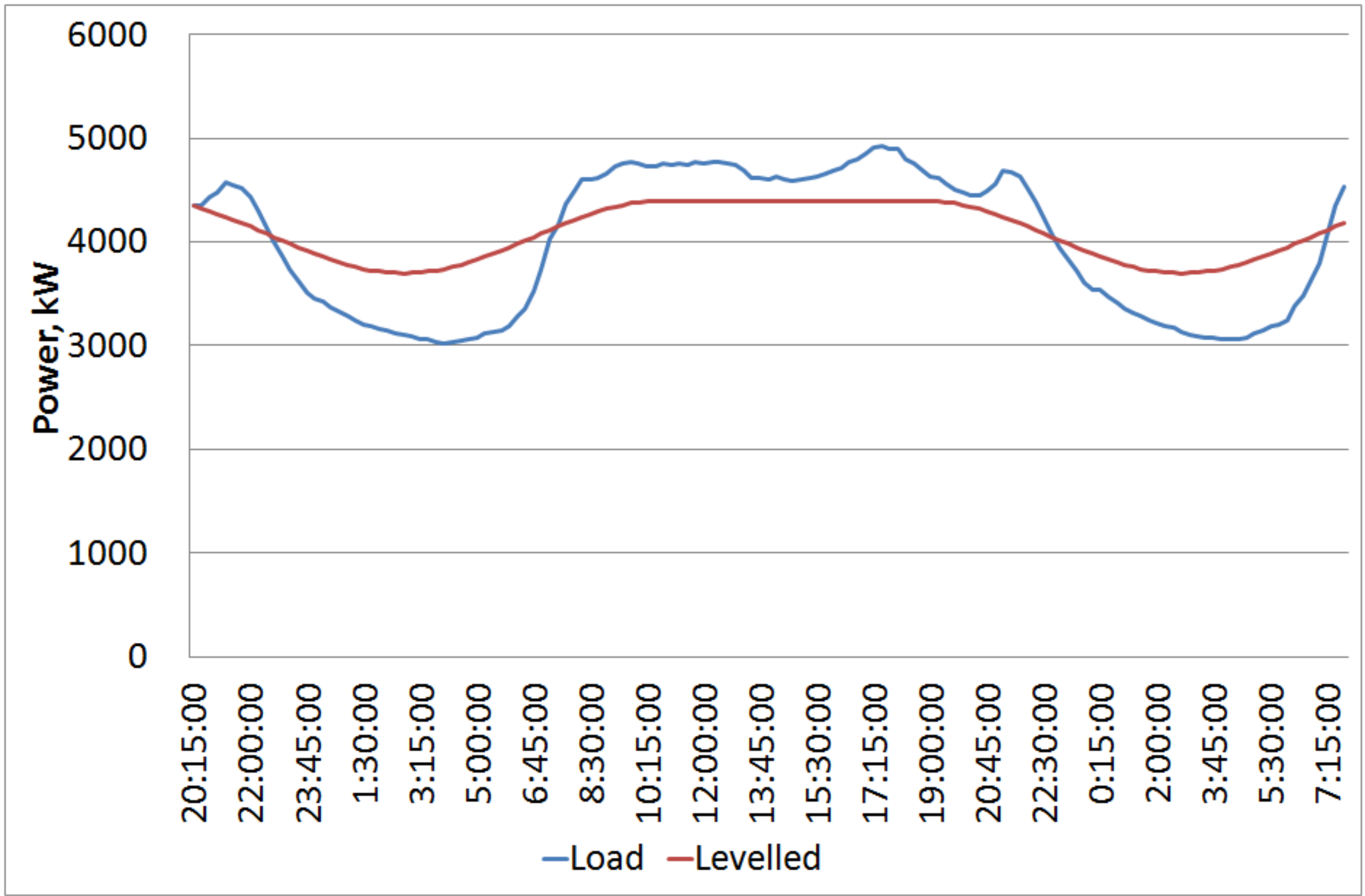
Figure 1: Leveled load on Ireland data

In the calculations of the charging/discharging strategy, we used a piece-wise specified core for the efficiency of the storage components:

$$K(t,s)=\left\{\begin{array}[]{ll}\mbox{$1,\,\,0<s<t/4,$}\\ \mbox{$0.9,\,\,t/4<s<3t/4,$}\\ \mbox{$0.85,\,\,3t/4<s<3t.$}\\ \end{array}\right.$$

Since the data on the load and its forecasts are given in tabular form, we used the approximations of load and its forecasts by a 4th degree polynomials by 10 points for solving Volterra integral equation by Taylor collocations. The result of the work on accurate and forecast data is shown in the figure (2). Here alternating changing power functions (ACPF) show charge and discharge strategies.

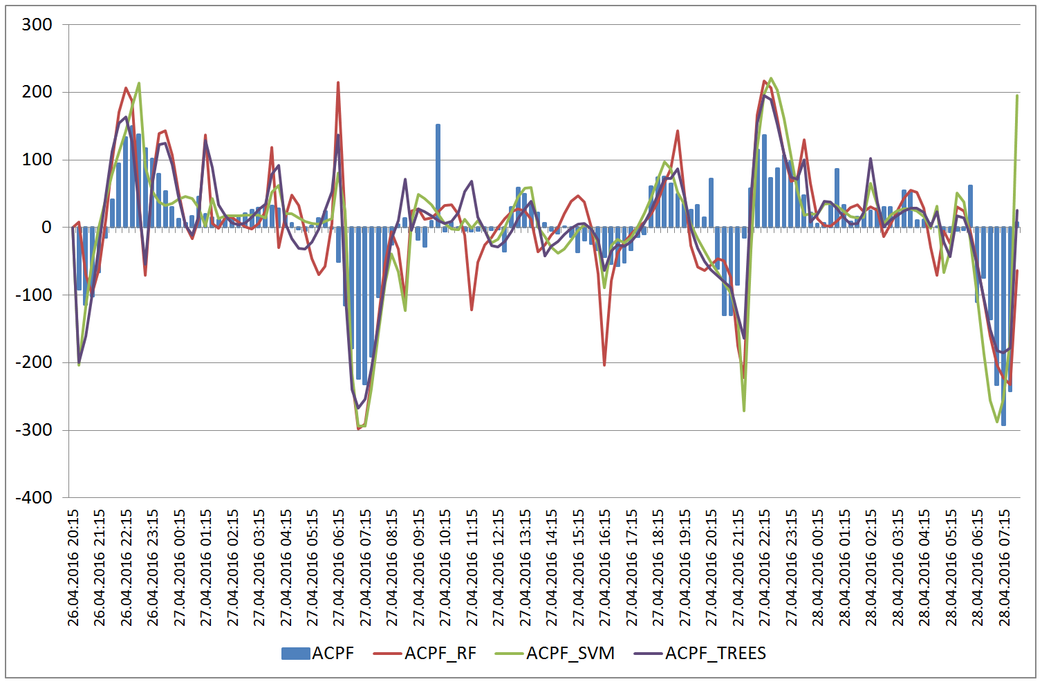
Figure 2: Charge/discharge strategies using various 24- hour forecasts and calculated by Taylor-collocation method

The Taylor collocation method has similar results to the spline collocation method as shown in the figure (3).

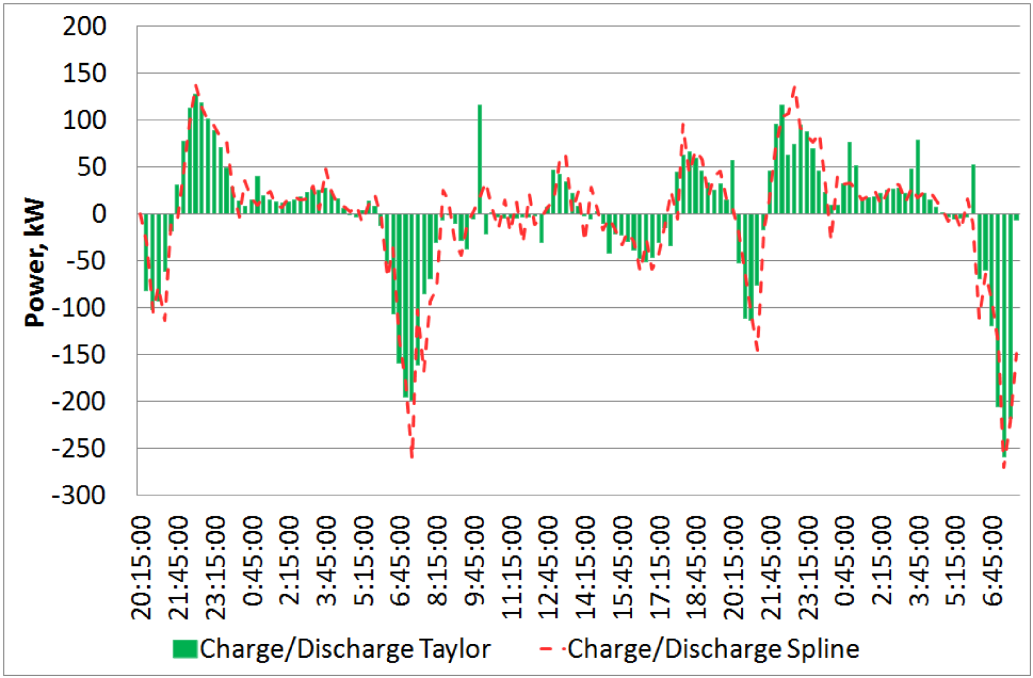
Figure 3: Charge/discharge strategies based on Taylor-collocation method and strategy spline collocations (bars)

The state of charge (SoC) calculated by these methods is shown in the figure (4). The difference between SoC values can be explained by the polynomial approximation of the right side of the Volterra integral equation for the Taylor-collocation method.

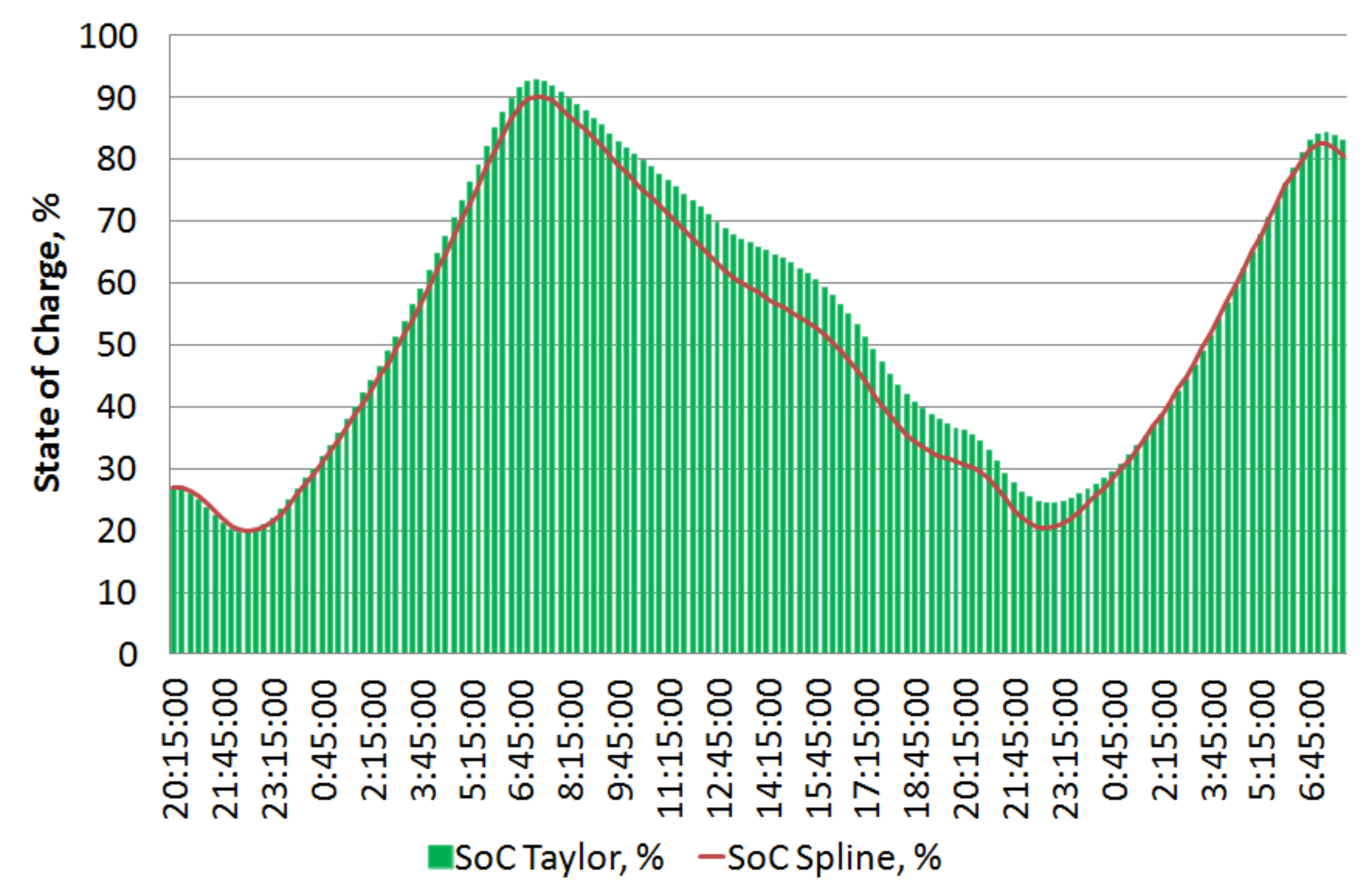
Figure 4: State of charge calculated by Taylor-collocation method and spline collocations

Table 1: Numerical results based on the CESTAC method for $f_{8}$.

$n$	$v_{n}(t)$	$|v_{n}-v_{n+1}(t)|$
2	0.10082463733333E+003	0.10082463733333E+003
3	0.10841798623809E+003	0.7593348904761E+001
4	0.1122562709626E+003	0.38382847245E+001
5	0.11218760890E+003	0.68662057E-001
6	0.1121987347E+003	0.111258E-001
7	0.112198015E+003	0.7190E-003
8	0.1121979E+003	0.9E-004
9	0.112197E+003	@.0

In order to apply the CESTAC method to find the optimal approximation, the optimal error and the step of Taylor-collocation method, one of inputed values $f_{i}$ is chosen. Then the presented method is applied to solve the Eq. (2.4) based on the CESTAC method. In this example, the 8-th value of $f_{i}$ is chosen and the numerical results of Table 1 are obtained. According to these results, the optimal step of charging/discharging strategies to find the 8-th value of them is $n=9$, the optimal approximation is $v_{9}=0.112197E+003$ and the optimal error is $0.9E-004$. According to Theorem 2, the NCSDs of exact and approximate solutions are equal to the NCSDs of two successive approximations. So we do not need to existence the exact solution and instead of applying the termination criterion (2.5) we apply the stopping condition (2.6).

4 Conclusion

This paper develops further the mathematical methodology employed in [25]for the first multi-vector energy analysis for the interconnected energy systems of Great Britain and Ireland. The efficient numerical method is designed and applied to the load leveling problem. Its efficiency is demonstrated on the real retrospective data of the Single Electricity Market (SEM) of the Island of Ireland. It is to be noted that employed evolutionary dynamical models are able to take into account (in terms of Volterra jump discontinuous kernels) both the time-dependent efficiency and the availability of generation/storage of each energy storage technology in the power system. The considered SEM is a power system with high wind power penetration and much unpredictability due to the inherent variability of wind. Following [25], the problem of efficient charge/discharge strategies is reduced to solving integral equations and their systems. The novel numerical methods using stochastic arithmetic and Taylor-collocation are proposed for such equations to find the available storage dispatch schedules. The convergence theorem is proved for the designed method of IE solution. The proposed method is applied to real data demonstrating its effectiveness.

Samad Noeiaghdam, PhD, Associate professor, Baikal School of BRICS, Irkutsk National Research Technical University, Lermontov st. 83, Irkutsk, 664074, Russian Federation; South Ural State University, Lenin prospect 76, Chelyabinsk, 454080, Russian Federation

Denis Sidorov, Doctor of Sciences (Physics and Mathematics), Pro-fessor, Melentiev Energy Systems Institute SB RAS, 130, Lermontov st., Irkutsk, 664033, Russian Federation, tel.: (3952) 500-646 ext. 258; Irkutsk National Research Technical University, Lermontov st. 83, Irkutsk, 664074, Russian Federation; Irkutsk State University, K. Marx st. 1, Irkutsk, 664003, Russian Federation

Ildar Muftahov, Programmer, Irkutsk Computing Center of Joint Stock Company Russian Railways, Mayakovaskii st. 25, Irkutsk, 664005, Russian Federation; Melentiev Energy Systems Institute SB RAS, 130, Lermontov st., Irkutsk, 664033, Russian Federation

Aleksei Zhukov, Junior research fellow, Institute of Solar-Terrestrial Physics SB RAS, 126a, Lermontov st., Irkutsk, 664033, Russian Federation; Melentiev Energy Systems Institute SB RAS, 130, Lermontov st., Irkutsk, 664033, Russian Federation

 

Контроль точности метода коллокаций Тейлора для задачи выравнивания нагрузки

Нойягдам Самад

Сидоров Денис Николаевич

Муфтахов Ильдар Ринатович

Жуков Алексей Витальевич

Abstract. Высокая степень проникновения возобновляемых источников энергии в сочетании с децентрализацией транспортных и тепловых нагрузок в будущих энергосистемах приведет к еще более сложному решению проблемы энергозатрат с учетом планирования аккумулирования энергии для эффективного выравнивания нагрузки. В данной статье рассматривается адаптивный подход к задаче выравнивания нагрузки с использованием интегральных динамических моделей Вольтерра. Задача формулируется как решение интегрального уравнения Вольтерра первого рода, которое решается с помощью численного метода коллокаций Тейлора, имеющего точность второго порядка и обладающего свойствами саморегуляции, что связано с доверительными уровнями системного спроса. Также применяется метод CESTAC для нахождения оптимальной аппроксимации, оптимальной погрешности и оптимального шага метода коллокаций. Данный адаптивный подход подходит для оптимизации накопления энергии в режиме реального времени. Эффективность предлагаемой методики продемонстрирована на едином рынке электроэнергии острова Ирландия.

Keywords: задача выравнивания нагрузки; метод коллокаций Тейлора; стохастическая арифметика; метод CESTAC

Нойягдам Самад, PhD, доцент, Иркутский национальный исследовательский технический университет, 664074, г. Иркутск, ул. Лермонтова, 83, Российская Федерация; Южно-Уральский Государственный Университет, 454080, г. Челябинск, Проспект Ленина, 76, Российская Федерация .

Сидоров Денис Николаевич, доктор физико-математических наук, профессор РАН, Институт систем энергетики им. Л.А.Мелентьева СО РАН, 664033, Иркутская область, г. Иркутск, ул. Лермонтова, д. 130, тел.: (3952)500-646 (код 258), Российская Федерация; Иркутский национальный исследовательский технический университет, 664074, г. Иркутск, ул. Лермонтова, 83, Российская Федерация; Иркутский государственный университет, 664003, Иркутск, ул. К. Маркса, 1, Российская Федерация .

Муфтахов Ильдар Ринатович, программист, Иркутский инфор-мационно-вычислительный центр ОАО <<РЖД>>, 664005, г. Иркутск, ул. Маяковского, 25, Российская Федерация; Институт систем энергетики им. Л. А. Мелентьева СО РАН, 664033, г. Иркутск, ул. Лермонтова, 130, Российская Федерация .

Жуков Алексей Витальевич, младший научный сотрудник, Институт солнечно-земной физики СО РАН, 664033, Иркутская область, г. Иркутск, ул. Лермонтова, д. 126a, Российская Федерация; Институт систем энергетики им. Л. А. Мелентьева СО РАН, 664033, г. Иркутск, ул. Лермонтова, 130, Российская Федерация.

References

- [1] Abbasbandy S., Fariborzi Araghi M.A. The use of the stochastic arithmetic to estimate the value of interpolation polynomial with optimal degree. Appl. Numer. Math., 2004, vol. 50, pp.279–290.
- [2] Abbasbandy S., Fariborzi Araghi M.A. A stochastic scheme for solving definite integrals. Appl. Numer. Math., 2005, vol. 55, 125–136.
- [3] -J.M. Chesneaux, Study of the computing accuracy by using probabilistic approach, in: C. Ullrich (Ed.), Contribution to Computer Arithmetic and Self-Validating Numerical Methods, IMACS, New Brunswick, NJ, (1990).
- [4] Dag I., Canivar A., Sahin A. Taylor–Galerkin and Taylor–collocation methods for the numerical solutions of Burgers’ equation using B-splines. Communications in Nonlinear Science and Numerical Simulation, 2011, vol. 16 (7), pp. 2696–2708.
- [5] Davies Penny J., Duncan Dugald B. Numerical approximation of first kind Volterra convolution integral equations with discontinuous kernels. Journal of Integral Equations and Applications, 2017, vol. 29 (1), pp. 41–73.
- [6] Enesiz Y., Keskin Y., Kurnaz A. The solution of the Bagley–Torvik equation with the generalized Taylor collocation method. Journal of the Franklin Institute, 2010, vol. 347 (2), pp. 452–466.
- [7] Fariborzi Araghi M.A., Noeiaghdam S. A novel technique based on the homotopy analysis method to solve the first kind Cauchy integral equations arising in the theory of airfoils. Journal of Interpolation and Approximation in Scientific Computing, 2016, vol. 1, pp. 1–13.
- [8] Fariborzi Araghi M.A., Noeiaghdam S. Fibonacci-regularization method for solving Cauchy integral equations of the first kind. Ain Shams Eng J., 2017, vol. 8, pp. 363–369. DOI:10.1016/j.asej.2015.08.018
- [9] Fariborzi Araghi M.A., Noeiaghdam S. Dynamical control of computations using the Gauss-Laguerre integration rule by applying the CADNA library. Advances and Applications in Mathematical Sciences, 2016, vol. 16, pp. 1–18.
- [10] Fariborzi Araghi M.A., Noeiaghdam S. A valid scheme to evaluate fuzzy definite integrals by applying the CADNA library. International Journal of Fuzzy System Applications, 2017, vol. 6 (4), pp. 1–20.
- [11] Gokmen E., Isik O. Rasit, Sezer M. Taylor collocation approach for delayed Lotka–Volterra predator-prey system. Applied Mathematics and Computation, 2015, vol. 268, pp. 671–684.
- [12] Gu Y., Xu J., Chen D., Wang Z., Li Q. Overall review of peak shaving for coal-fired power units in China. Renewable and Sustainable Energy Reviews, 2016, vol. 54, pp. 723–731.
- [13] Muftahov I., Tynda A., Sidorov D. Numeric Solution of Volterra Integral Equations of the First Kind with Discontinuous Kernels. Journal of Computational and Applied Mathematics, 2017, vol. 313, pp. 119–128.
- [14] Muftahov I. R., Sidorov D. N. Solvability and numerical solutions of systems of nonlinear Volterra integral equations of the first kind with piecewise continuous kernels. Vestnik YuUrGU. Ser. Mat. Model. Progr., 2016, vol. 9 (1), 130–136.
- [15] Noeiaghdam S., Fariborzi Araghi M.A. Finding optimal step of fuzzy Newton-Cotes integration rules by using the CESTAC method. Journal of Fuzzy Set Valued Analysis, 2017, vol. 2, pp. 62–85.
- [16] Noeiaghdam S., Fariborzi Araghi M. A., Abbasbandy S. Finding optimal convergence control parameter in the homotopy analysis method to solve integral equations based on the stochastic arithmetic. Numer Algor, 2019, vol. 81 (1), pp. 237–267. https://doi.org/10.1007/s11075-018-0546-7
- [17] Noeiaghdam S., Sidorov D., Sizikov V. Control of accuracy on Taylor-collocation method to solve the weakly regular Volterra integral equations of the first kind by using the CESTAC method. arXiv:1811.09802.
- [18] Noeiaghdam S., Zarei E., Kelishami H. Barzegar. Homotopy analysis transform method for solving Abel’s integral equations of the first kind. Ain Shams Eng J., 2016, vol. 7, pp. 483–495.
- [19] Pazouki S., Haghifam M.-R. Optimal planning and scheduling of energy hub in presence of wind, storage and demand response under uncertainty. International Journal of Electrical Power & Energy Systems, 2016, vol. 80, pp. 219–239.
- [20] Sezer M., Gülsu M. Polynomial solution of the most general linear Fredholm–Volterra integrodifferential-difference equations by means of Taylor collocation method. Applied Mathematics and Computation, 2007, vol. 185(1), pp. 646–657.
- [21] Sidorov D.N. On Parametric Families of Solutions of Volterra Integral Equations of the First Kind with Piecewise Smooth Kernel. Differential Equations, 2013, vol. 49(2), pp. 210–216.
- [22] Sidorov D., Muftahov I., Tomin N., Karamov D., Panasetsky D., Dreglea A., Liu F. A dynamic analysis of energy storage with renewable and diesel generation using Volterra equations. IEEE Transactions on Industrial Informatics, 2019. DOI:10.1109/TII.2019.2932453
- [23] Sidorov N.A., Sidorov D.N. On the Solvability of a Class of Volterra Operator Equations of the First Kind with Piecewise Continuous Kernels. Mathematical Notes, 2014, vol. 96(5), pp. 811–826.
- [24] Sidorov D.N., Tynda A.N., Muftahov I.R. Numerical solution of Volterra integral equations of the first kind with piecewise continuous kernel. Vestnik YuUrGU. Ser. Mat. Model. Progr., 2014, vol. 7(3), pp. 107–115.
- [25] Sidorov D., Zhukov A., Foley A., Tynda A., Muftahov I., Panasetsky D., Li Y. Volterra models in load levelling problem. E3S Web of Conference, 2018, vol. 69, 01015, pp.1–6. DOI:10.1051/e3sconf/20186901015
- [26] Sizikov V., Sidorov D. Generalized quadrature for solving singular integral equations of Abel type in application to infrared tomography. Appl. Numer. Math., 2016, vol. 106, pp. 69–78.
- [27] Sizikov V.S., Smirnov A.V., Fedorov B.A. Numerical solution of the Abelian singular integral equation by the generalized quadrature method. Rus. Math. (Iz. VUZ), 2004, vol. 48 (8), pp. 59–66.
- [28] Soares L., Medeiros M. Modeling and forecasting short-term electricity load: a comparison of methods with an application to Brazilian data. Int. J. Forecast, 2008, vol. 24, pp. 630–644.
- [29] System Operator of Northern Ireland. http://www.soni.ltd.uk/Operations/sg/DS3/. Accessed: 2016-01-07.
- [30] Verlan A.F., Sizikov V.S. Integral Equations: Methods, Algorithms, Programs. Nauk. Dumka, 1986.
- [31] Vignes J. A stochastic arithmetic for reliable scientific computation. Math. Comput. Simulation, 1993, vol. 35, pp. 233–261.
- [32] Zakeri B., Syri S. Electrical energy storage systems: A comparative life cycle cost analysis. Renewable and Sustainable Energy Reviews, 2015, vol. 42, pp. 569–596.