Multidataset Independent Subspace Analysis
with Application to Multimodal Fusion

Abstract

In the last two decades, unsupervised latent variable models—blind source separation (BSS) especially—have enjoyed a strong reputation for the interpretable features they produce. Seldom do these models combine the rich diversity of information available in multiple datasets. Multidatasets, on the other hand, yield joint solutions otherwise unavailable in isolation, with a potential for pivotal insights into complex systems.

To take advantage of the complex multidimensional subspace structures that capture underlying modes of shared and unique variability across and within datasets, we present a direct, principled approach to multidataset combination. We design a new method called multidataset independent subspace analysis (MISA) that leverages joint information from multiple heterogeneous datasets in a flexible and synergistic fashion.

Methodological innovations exploiting the Kotz distribution for subspace modeling in conjunction with a novel combinatorial optimization for evasion of local minima enable MISA to produce a robust generalization of independent component analysis (ICA), independent vector analysis (IVA), and independent subspace analysis (ISA) in a single unified model.

We highlight the utility of MISA for multimodal information fusion, including sample-poor regimes and low signal-to-noise ratio scenarios, promoting novel applications in both unimodal and multimodal brain imaging data.

I Introduction

Blind source separation ( blind source separation (BSS)) [1, 2] is widely adopted across multiple research areas in signal, image, and video processing, including chemometrics [3], speech [4], multispectral imaging [5, 6], medical imaging [7, 8], and video processing [9, 10]. The “blind” property of BSS models is highly advantageous, especially in applications lacking a precise model of the measured system(s) and with data confounded by noise of unknown or variable characteristics. Its popularity has led to many formulations, methodologies, and algorithmic variations, at times making it difficult to build clear intuition about their connections and, thus, impeding further development toward flexible, more general models.

Figure 1: Subspace identification from multidatasets with MISA. We consider the general case of $M$ datasets ($\mathbf{x}_{m}$) jointly decomposed, without loss of generality, into $C$ sources $y_{mi}$ each, via linear transformations $\mathbf{W}_{m}$. Here, each $\mathbf{x}_{m}$ would be either audio or video streams, indicating fusion of different modalities via the joint analysis of all datasets. Sources are combined into $d_{k}$-dimensional subspaces $\mathbf{y}_{k}$ and all-order statistics is utilized to gauge their associations and pursue subspace independence. Only a single correspondence “axis” is required to make these assessments, such as temporal alignment in the case of audio/video (a/v) data fusion, although the method is not limited to a/v, fusion, nor temporal alignment specifically. Subspaces establish links among groups of sources across different datasets/modalities. Therefore, multidataset independent subspace analysis (MISA) blindly recovers hidden linked features of flexible dimensionality from multiple datasets and modalities.

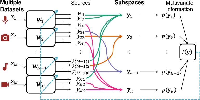
In our recent review [1], we addressed this issue by introducing a novel multidataset multidiversity multidimensional (MMM) unified modeling framework (UMF) for subspace modeling. This helped us organize the BSS field while casting new light on the relationships among BSS models, eventually reconciling research conducted on both single-dataset multidimensional (SDM) and multidataset unidimensional (MDU) problems. The proposed framework revealed several development directions emphasizing new ways to identify general subspace correspondence across datasets, coined therein as multidataset multidimensional (MDM) problems.

Owing to their inherent flexibility, models designed for MDM problems are highly advantageous. With a single joint model, it is possible to not only encode higher complexity through features of flexible dimensionality (the subspaces $\mathbf{y}_{k}$) but also accommodate arbitrary links among these features over multiple datasets/modalities ($\mathbf{x}_{m}$). To illustrate, (Fig. 1) we consider a multivariate information functional $I(\mathbf{y})$ that operates simultaneously on the joint probability density functions of all subspaces $p(\mathbf{y}_{k})$, capturing the association modes underlying multidatasets while adaptively learning multiple linear transformations $\mathbf{W}_{m}$ (dashed lines). This directly leverages multidataset joint information and lets it guide the decomposition naturally.

MDM problems constitute a largely undeveloped area of research with great potential to impact many fields. In classification, short of instances affected by the curse of dimensionality, multidimensional features are prone to yield better results, often owing to the increased feature space size. The association/dependence inherent to multimodal features $\mathbf{y}_{k}$ means that good separability in one dataset will promote features with similar property in other datasets, and vice-versa.

In multimodal fusion of heterogeneous data ($\mathbf{x}_{m}$) [11, 12], robust identification of joint features that originate from all data modalities offers a one-of-a-kind view into the underlying properties of the system at hand. It is a highly promising direction in mental health research, owing to its potential to identify biological markers of disease for early diagnosis, as well as to convey new strategies for disease severity assessment and translation into personalized treatments [1]. Insights about the organization and function of complex systems, including the human brain, are indeed highly desirable.

The elevated flexibility of MDM models would also be highly beneficial to various multiset analyses. In the case of multisubject unimodal data ($\mathbf{x}_{m}$) [13, 14, 15, 16, 17, 18], it would better preserve subject specificity. In analyses that combine multi-site datasets ($\mathbf{x}_{m}$) from different scanners/devices, it could naturally mitigate harmonization issues [19, 20] since site/device-variability would seldom explain multidataset associations. In sensor fusion [11, 21, 22, 5], where noise characteristics can be similar if multiple sensors ($\mathbf{x}_{m}$) share the same environment, it would allow better detection (and potential removal) of noise. For hyperspectral imaging [23, 24, 25], hyperspectral features ($\mathbf{y}_{k}$) of higher complexity could be identified in time-lapse studies. For domain-adaptive image recognition [26, 27, 28, 29, 30], enhanced common and unique representations ($\mathbf{y}_{k}$) could be identified across image domains ($\mathbf{x}_{m}$). For multi-view image and video processing [9, 31, 32], objects with complex temporal patterns could be better characterized using (unimodal) higher-dimensional $\mathbf{y}_{k}$, not to mention potential fusion with audio features [33, 34, 35, 36] via multimodal $\mathbf{y}_{k}$.

Therefore, aiming to tackle the more general case of MDM models that pursue statistical independence among subspaces $\mathbf{y}_{k}$ to achieve joint BSS, we initially introduced a solution called MISA in [37, 38, 39], demonstrating its feasibility, potential, and generalization. While novel, this preliminary version, to which we now refer as $\alpha$-MISA, lacked robustness and performance across subspace configurations $\mathbf{P}$ (Fig. 2) due to premature convergence to local minima, rigid hard-coded subspace joint pdf parameters, and a restricted approach for regularization of $\mathbf{W}_{m}$.

Here, we propose to address these issues by utilizing combinatorial optimization to search over $\mathbf{P}$, as well as all-order statistics (i.e., both second- and higher-order statistics, SOS and HOS, respectively) to model $p(\mathbf{y}_{k})$ and solve the MDM problem while identifying statistically independent subspaces $\mathbf{y}_{k}$, referring to this improved approach simply as MISA (Fig. 1). Following Figs. 1 and 2, let $p\left(\mathbf{y}\right)$ represent the joint pdf of all sources, and $p(\mathbf{y}_{k})$ the pdf of the $k$-th subspace.

Let $I(\mathbf{y})$ be the Kullback-Leibler (KL) divergence, an information functional useful for comparing two pdfs $p(\mathbf{y})$ and $q(\mathbf{y})$, where, here, $q\left(\mathbf{y}\right)=\prod_{k=1}^{K}p(\mathbf{y}_{k})$ is the desired factor pdf of $p(\mathbf{y})$. Then let $h(\cdot)$ be the joint differential entropy, $h(\mathbf{z})=-\mathbb{E}\left[\ln p(\mathbf{z})\right]$, for a random vector $\mathbf{z}$ with pdf $p(\mathbf{z})$, $\mathbb{E}\left[\cdot\right]$ being the expected value operator, and let $\mathbf{P}_{k}$ be an incomplete permutation matrix that assigns specific sources into subspace $k$. Consequently, it follows that:

We propose to estimate a collection of linear transformations $\mathbf{y}=\mathbf{W}\mathbf{x}$ simultaneously from all datasets by solving:

$$\min_{\mathbf{W},\>\mathbf{P}_{k}\forall k} I(\mathbf{y}),$$ (2)

for any $\mathbf{W}$, subspace assignments $\mathbf{P}_{k}$, and data streams $\mathbf{x}$. This convenient formulation, which gives mutual information (MI) when the random vector $\mathbf{y}$ is two-dimensional, only attains its lower bound of $I(\mathbf{y})=0$ when $p(\mathbf{y})=q(\mathbf{y})$, implying that the identified subspaces are indeed statistically independent.

With MISA, direct study of the interactions and associations among multiple datasets becomes feasible, in a truly synergistic way. Consequently, joint sources $\mathbf{y}_{k}$ emerge naturally as a direct result of the shared variability estimated from all-order statistical dependences among datasets, while breaking from the limited, rigid paradigms of unidimensional models in order to allow subspace associations and even absent features in specific datasets. Furthermore, as a unifying toolkit for independence-based MDM models, MISA not only takes the form of a single algorithm capable of executing any of the classical tasks as special cases, including independent component analysis (ICA) [40], independent subspace analysis (ISA) [41], and independent vector analysis (IVA) [42], in addition to many others, but also outperforms several algorithms in each of these tasks, successfully achieving generalized subspace identification from multidatasets. Having this uniform implementation makes model connections very intuitive and accessible, thanks to the umbrella formulation and methodologies introduced in this work.

Multiple experiments obeying the principles outlined in [43] demonstrate that MISA outperforms algorithms such as Infomax [44, 45], IVA Laplace (IVA-L) [42], and IVA Gaussian Laplace (IVA-GL) [46] in various challenging realistic scenarios, with remarkable performance and stability in certain extremely noisy cases (SNR of 0.0043dB), highlighting the benefit of careful multidataset subspace dependence modeling with all-order statistics. Likewise, MISA with greedy permutations (MISA-GP) clearly outperforms joint blind diagonalization with second-order statistics (SOS) (JBD-SOS) [47] and EST_ISA [48] even at low signal-to-noise ratio (SNR) levels (SNR of 3dB), highlighting the benefit of the proposed combinatorial optimization approach to escape local minima in subspace analyses. Hybrid data results further support the high estimation quality and flexibility benefits of MISA for novel applications in high-temporal-resolution functional MRI (fMRI) analysis, and multimodal fusion of heterogenous neurobiological signals.

II Background

II-A General MDM Problem Statement

BSS admits a hierarchical organization in accordance with the number of datasets comprising $\mathbf{x}$ and the occurrence of multidimensional sources (grouped subsets of $\mathbf{y}$) within any single dataset [1, 49, Ch. 8]. For example, MDU and SDM problems contain the simpler single-dataset unidimensional (SDU) case, and the most general MDM problem (see Fig. 2) contains all others as special cases.

Formally, the MDM problem can be stated as follows. Given $N$ observations of $M\geq 1$ datasets, identify an unobservable latent source random vector (r.v.) $\mathbf{y}=\left[\mathbf{y}_{1}^{\top}\cdots\mathbf{y}_{M}^{\top}\right]^{\top}$, $\mathbf{y}_{m}=[y_{m1}\cdots y_{mC_{m}}]^{\top}$, from an observed r.v. $\mathbf{x}=\left[\mathbf{x}_{1}^{\top}\cdots\mathbf{x}_{M}^{\top}\right]^{\top}$, $\mathbf{x}_{m}=[x_{1}\cdots x_{V_{m}}]^{\top}$ via a mixture vector function ${\bf f}\left(\mathbf{y},\bm{\theta}\right)$ with unknown parameters $\bm{\theta}$. The $m$-th $V_{m}\times N$ data matrix containing $N$ observations of $\mathbf{x}_{m}$ along its columns is denoted $\mathbf{X}_{m}$, and the $\bar{V}\times N$ matrix concatenating all $\mathbf{X}_{m}$ is denoted simply as $\mathbf{X}$ (likewise for $\mathbf{Y}$ and $\mathbf{Y}_{m}$). Both $\mathbf{y}$ and the transformation ${\bf f}\left(\mathbf{y},\bm{\theta}\right)$ have to be learned blindly, i.e., without explicit knowledge of either of them. For tractability, assume:

1. the number of latent sources $C_{m}$, which may differ in each dataset, is known to the experimenter;

2. ${\bf f}\left(\mathbf{y},\bm{\theta}\right)=\mathbf{A}\mathbf{y}$ is a linear transformation, with $\bm{\theta}=\mathbf{A}$;

3. $\mathbf{A}$ is a $\bar{V}\times\bar{C}$ block diagonal matrix with $M$ blocks, representing a separable layout structure [1] defined as $\mathbf{x}_{m}=\mathbf{A}_{m}\mathbf{y}_{m}$, $m=1\ldots M$, where $\bar{C}=\sum_{m=1}^{M}C_{m}$, $\bar{V}=\sum_{m=1}^{M}V_{m}$, each block $\mathbf{A}_{m}$ is $V_{m}\times C_{m}$, and $V_{m}$ is the intrinsic dimensionality of each dataset;

4. some latent sources $y_{mi}\in\mathbf{y}$ are statistically related to each other, and this dependence is undirected (non-causal), occurring within and/or across datasets;

5. related sources establish $d_{k}$-dimensional subspaces (or source groups) $\mathbf{y}_{k}$, $k=1\ldots K$, with $K$ and the specific subspace compositions known by the experimenter and listed in a sparse assignment matrix ${\mathbf{P}\in\{0,1\}^{K\times\bar{C}}}$ containing a single non-zero entry in each column;

6. subspaces do not relate to each other, i.e., either $p\left(\mathbf{y}\right)=\prod_{k=1}^{K}p(\mathbf{y}_{k})$ or the cross-correlations $\rho_{k,k^{\prime}}=0$, $k\neq k^{\prime}$.

Figure 2: General decompositional representation of the linear MDM problem. The lower layer corresponds to one $V_{m}\times 1$ observation of each input data stream $\mathbf{x}_{m}$. The middle layer represents the $C_{m}$ sources. The top layer establishes the $K$ subspaces $\mathbf{y}_{k}$, which are collections of statistically dependent sources (indicated by same-colored connections). They follow an assignment matrix $\mathbf{P}$, illustrating the different compositions permitted.

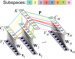
Under these assumptions, recovering sources $\mathbf{y}$ amounts to finding a linear transformation $\mathbf{W}$ for the unmixing vector function $\mathbf{y}=\mathbf{W}\mathbf{x}$. This is accurate when $\mathbf{W}=\mathbf{A}^{-}$, the pseudo-inverse of $\mathbf{A}$, which implies $\mathbf{W}$ is also block diagonal, thus satisfying $\mathbf{y}_{m}=\mathbf{W}_{m}\mathbf{x}_{m}$. As stated in [1], the experimenter’s priors on the subspace structure within/between one or more datasets, plus the type of statistics describing within/between subspace relation, determines whether and how the model simplifies to any of the special cases. In the following, we focus on the more general case of a MDM model driven by statistical independence among subspaces and dependence within subspaces, namely MISA, in the case of an overdetermined system with $V_{m}\geq C_{m}$, without implying $\mathbf{W}$ is square with the typical principal component analysis (PCA).

II-B Current Challenges and Our Contributions

Premature convergence to local minima due to the mis-assignment of sources to subspaces is a challenge for MDM model fitting. It has roots in ICA’s permutation ambiguity property that no particular ordering of the true independent sources alters their independence, in effect, describing a class of equivalent globally optimal solutions. While this property extends trivially to independent subspaces, arbitrary source permutations are no longer equivalent due to likely incorrect assignments of those sources into the subspaces. Hence, this is a key point that requires special attention.

To illustrate, assume $\mathbf{P}_{k}$ is a user-specified prior. Using abbreviated notation, suppose $\mathbf{P}_{1}=\left[1~{}1~{}1~{}0~{}0\right]$ and $\mathbf{P}_{2}=\left[0~{}0~{}0~{}1~{}1\right]$ defines a partitioning of five sources into two subspaces: $p(\mathbf{y})=p(\mathbf{y}_{k=1})p(\mathbf{y}_{k=2})=p(y_{1},y_{2},y_{3})p(y_{4},y_{5})$, where $p(\cdot)$ is the joint pdf of a subspace. It would be equally acceptable if the data supported either $p(\mathbf{y})=p(y_{4},y_{5})p(y_{1},y_{2},y_{3})$ (entire subspace permutation) or $p(\mathbf{y})=p(y_{1},y_{3},y_{2})p(y_{5},y_{4})$ (within-subspace permutation) or even some combination of these two cases. However, if the data supported $p(\mathbf{y})=p(y_{1},y_{4})p(y_{2},y_{3},y_{5})$, then that would not be equivalently acceptable. The latter characterizes a local minimum, while the former two constitute global minima.

In practice, these are hard-to-escape local minima [50]. In MISA, we have observed that a drastically more intricate joint interplay exists between within- and cross-dataset subspace-to-subspace interactions, which yields a combinatorial increase in number of these non-optimal local minima. Specifically, when subspaces span multiple datasets, very high $\prod_{k=1}^{K}{\bar{C}-\sum_{l=0}^{k-1}d_{l}\choose d_{k}}$ number of possible local minima (upwards of $6\cdot 10^{19}$ in Section IV-B4) cripples the numerical optimization performance (here, $d_{0}\triangleq 0$). Thus, we propose combinatorial optimization algorithms to enable evasion of local minima in the numerical optimization of (LABEL:eq:MISAprob).

While combinatorial issues are common in other research areas [51, 52, 53], they have been largely neglected in the BSS literature because of how simple (and often irrelevant) they are for ICA. To our knowledge, this is the first attempt at disentangling these permutation ambiguities in the general MISA case. Inspired by a strategy proposed in [54] for ISA, separate combinatorial optimization procedures to address general SDM and MDM problems are presented in Sections III-C and III-D, respectively. In contrast to [54], however, our approach does not rely on additional accessory objective functions to determine residual source dependences. Moreover, our approach leverages the structural subspace priors contained in $\mathbf{P}_{k}$ to guide the combinatorial procedures. Ultimately, the key difference is that our approach serves only to move a particular solution out of a local minima so that the numerical optimization may resume.

Another challenge stems from the distribution properties of $p(\mathbf{y}_{k})$. The a priori selection/hard-coding of distribution $p(\cdot)$ is common practice in BSS, often based on some domain knowledge about source properties, e.g., sub- or super-Gaussian attributes [44, 55]. Likewise, the subspace covariance structure $\bm{\Sigma}_{k}^{\mathbf{y}}$ is often hard-coded to identity (i.e., uncorrelated) [56, 16] or just iteratively substituted with data estimates [57, 46] in MDU and SDM problems. While these practices facilitate tractability (also the case in our previous work) they curb generalization beyond the context of model conception and can altogether fail to capture the subspace structure supported by the data. Even objective function gradients can become inconsistent in the case of simple iterative substitution, despite its intent to encourage data-supported dependences.

In order to help counter the rigidity and immutability of said choices, we pursue the use of a generalized pdf [58, 42, 59] that includes additional parameters to better cater for sources that the data supports, as suggested in [60, Sec. 3.3.2] and adopted in [61] for ICA. Following [57], we introduce the Kotz distribution [58] for MISA due to its generality, as it includes the multivariate power exponential family as a special case. Contrary to approaches based on the multivariate Gaussian [47, 62, 63], which incorporates only SOS, and the multivariate Laplace (with uncorrelated subspace covariance $\bm{\Sigma}_{k}^{\mathbf{y}}=\mathbf{I}$, incorporating only higher-order statistics (HOS)) [56, 16, 39], the Kotz distribution can account for both and enable all-order statistics. Moreover, we extend [57] in two ways: 1) we address the MDM case rather than just the MDU case, and 2) we improve performance considerably by casting $\bm{\Sigma}_{k}^{\mathbf{y}}$ as a direct function of the linear transformation parameter being optimized, namely $\mathbf{W}$, into $p(\mathbf{y}_{k})$, rather than treating it as constant with respect to $\mathbf{W}$ in spite of its iterative updates.

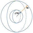
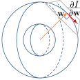
Finally, there is a challenge with source scale estimation. The property of independence between sources is inherently invariant to arbitrarily scaling each or any source, which is why ICA sources have scale ambiguity. This has an important implication on the geometry of the resulting objective function we seek to optimize. First, visualize the elements of $\mathbf{W}$ into a $\bar{D}$-dimensional vector ($\bar{D}=\bar{V}\bar{C}$) $\mathbf{w}=\operatorname{vec}{(\mathbf{W})}$ as would be done in a typical numerical optimization setting. Due to scale invariance, evaluation of the objective function on either $\mathbf{w}$ or $a\mathbf{w}$, where $a$ is a non-zero scalar, yields the same value.

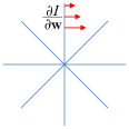
Since the objective function evaluates to the same values along the line spanned by $\mathbf{w}$, only certain changes in the direction of $\mathbf{w}$ incur changes in the objective function. Consequently, it suffices to look for a solution on the surface of the hypersphere associated with a given $a$, since the landscape of objective function values would be identical across concentric (hyper) shells (Fig. 3 (a)). Moreover, scale invariance induces a “star” shape to the contour lines of the objective function in this scenario (Fig. 3 (b)). Since gradients are orthogonal to contour lines, they also ought to be orthogonal to $\mathbf{w}$ and lie on the tangent hyperplane of any given hypersphere (Fig. 3 (c)).

The main implication is that stepping in the (negative) direction of the gradient towards a local minimum will likely inflate $\mathbf{w}$ and lead the search direction in an outward spiral with respect to $\mathbf{w}$. This can be a problem if the norm of $\mathbf{w}$ grows indefinitely and eventually becomes numerically unstable. More importantly, as the norm of $\mathbf{w}$ increases toward outer shells, the landscape of the objective function starts to stretch (because its values are kept the same while the surface area of the hypersphere grows). Consequently, the gradient grows shorter regardless of its proximity to any local minimum. The smaller gradient will then lead to shorter step lengths, likely yielding very little improvement at latter stages of the numerical optimization and deterring convergence.

(a) Concentric hyperspheres

(b) Contour lines

(c) Tangent plane

Figure 3: Geometry of the independence-driven objective function in SDU problems. (a) The solution space of independence-driven SDU problems lies on a hypersphere. (b) Scale invariance induces a “star” shape on the contour lines. (c) Consequently, the gradient of a scale invariant function must lie on the tangent hyperplane of the hypersphere associated with a given $\mathbf{w}$.

This issue is often disregarded in the SDU literature (the Infomax algorithm [44] is an exception) and should be addressed prior to evaluation of the efficient relative gradient [2, Ch. 4]. One simple approach to address it is to constrain the norm of $\mathbf{w}$. While direct, implementing this approach can be quite inefficient. Rather, since any scale is equally acceptable (at least in theory), we propose to control the estimated source scales by fixing them in the model. Specifically, this is accomplished by assigning the estimated subspace correlation matrix $\mathbf{R}^{\mathbf{y}}_{k}$ as the model dispersion matrix $\mathbf{D}_{k}$ in the Kotz distribution, effectively making the objective function scale selective rather than scale invariant (Section III-A). Therefore, whenever the source estimates from the data do not support the model variances associated with this choice of $\mathbf{D}_{k}=\mathbf{R}^{\mathbf{y}}_{k}$, the mismatch induces changes in $\mathbf{W}$ that lead their variances towards the prescribed ones. In summary, the proposed scale selective formulation eliminates scaling issues without the need for a formal constraint.

We also introduce the pseudo-inverse reconstruction error (PRE) as a nonlinear constraint for estimation of rectangular non-invertible mixing matrices (also serving as a flexible alternative for data reduction), and utilize quasi-newton optimization based on the relative gradient for efficient optimization.

III Methodology

III-A Objective Function

Equation (LABEL:eq:MISAprob) admits some simplifications following a few manipulations. First, we note that $h(\mathbf{y})=h(\mathbf{W}\mathbf{x})=h(\mathbf{x})+\ln\left|\det(\mathbf{W})\right|$, and $h(\mathbf{x})$ can be discarded since it is constant with respect to $\mathbf{W}$. Second, $\ln\left|\det(\mathbf{W})\right|=\sum_{m=1}^{M}\ln\left|\det(\mathbf{W}_{m})\right|$ since $\mathbf{W}$ is block diagonal. Finally, when $V_{m}\neq C_{m}$, for any $m$, the determinant of $\mathbf{W}_{m}$ is undefined. In order to circumvent this issue, we propose to substitute the determinant by the product of the singular values of $\mathbf{W}_{m}$, i.e., $\prod_{i=1}^{C_{m}}\sigma_{mi}$, where $\sigma_{mi}$ are the diagonal elements of $\bm{\Lambda}_{m}=\mathbf{U}_{m}^{\top}\mathbf{W}_{m}\mathbf{V}_{m}$ originating from the singular value decomposition $\mathbf{W}_{m}=\mathbf{U}_{m}\bm{\Lambda}_{m}\mathbf{V}_{m}^{\top}$. We note that $\left|\det\mathbf{W}\right|=\prod_{i=1}^{C}\left|\sigma_{mi}\right|$ when $\mathbf{W}$ is non-singular and square. Altogether, the minimization problem can then be recast as:

$$\min_{\mathbf{W},\mathbf{P}_{k}\forall k} \>\>\check{I}(\mathbf{y}),\>\>\check{I}(\mathbf{y})=-\sum_{m=1}^{M}J_{D_{m}}-\sum_{k=1}^{K}\mathbb{E}\left[\ln p(\mathbf{y}_{k})\right]\mathrm{,}$$ (3)

where $J_{D_{m}}=\sum_{i=1}^{C_{m}}\ln\left|\sigma_{mi}\right|$, and $\mathbf{y}_{k}=\mathbf{P}_{k}\mathbf{W}\mathbf{x}$.

This formulation is still incomplete because $p(\mathbf{y}_{k})$ is undefined. Here we choose to model each subspace pdf as a multivariate Kotz distribution [64, 58]:

$$p(\mathbf{y}_{k})=\frac{\beta_{k}\lambda_{k}^{\nu_{k}}\Gamma\left(\frac{d_{k}}{2}\right)\left(\mathbf{y}_{k}^{\top}\mathbf{D}_{k}^{-1}\mathbf{y}_{k}\right)^{\eta_{k}-1}}{\pi^{\frac{d_{k}}{2}}\left(\det\mathbf{D}_{k}\right)^{\frac{1}{2}}\Gamma\left(\nu_{k}\right)}e^{-\lambda_{k}\left(\mathbf{y}_{k}^{\top}\mathbf{D}_{k}^{-1}\mathbf{y}_{k}\right)^{\beta_{k}}}$$ (4)

where $d_{k}$ is the subspace dimensionality, $\beta_{k}>0$ controls the shape of the pdf, $\lambda_{k}>0$ the kurtosis (i.e., the degree of peakedness), and $\eta_{k}>\frac{2-d_{k}}{2}$ the hole size, while $\nu_{k}\triangleq\frac{2\eta_{k}+d_{k}-2}{2\beta_{k}}>0$ and $\alpha_{k}\triangleq\frac{\Gamma\left(\nu_{k}+\beta_{k}^{-1}\right)}{\lambda_{k}^{\beta_{k}^{-1}}d_{k}\Gamma\left(\nu_{k}\right)}$ for brevity. $\Gamma\left(\cdot\right)$ denotes the gamma function. The positive definite dispersion matrix $\mathbf{D}_{k}$ is related to the covariance matrix $\bm{\Sigma}_{k}^{\mathbf{y}}$ by ${\mathbf{D}_{k}=\alpha_{k}^{-1}\bm{\Sigma}_{k}^{\mathbf{y}}}$. This is a good choice of pdf since it generalizes and includes other classical distributions such as the multivariate Gaussian and the multivariate Laplace distributions by setting the pdf parameter set $\bm{\psi}_{k}=[\beta_{k},\lambda_{k},\eta_{k}]$ to $\bm{\psi}_{G}=[1,\frac{1}{2},1]$ and $\bm{\psi}_{L}=[\frac{1}{2},1,1]$, respectively. The second term in (3) admits the following form:

$$\ln p(\mathbf{y}_{k})=\ln\left(\frac{\beta_{k}\lambda_{k}^{\nu_{k}}\Gamma\left(\frac{d_{k}}{2}\right)}{\pi^{\frac{d_{k}}{2}}\Gamma\left(\nu_{k}\right)}\right)+\frac{(\eta_{k}-1)J_{F_{k}}}{\frac{1}{2}J_{C_{k}}}-\lambda_{k}J_{E_{k}}$$ (5)

where $J_{C_{k}}=\ln\det\mathbf{D}_{k}$, $J_{F_{k}}=\ln\left(\mathbf{y}_{k}^{\top}\mathbf{D}_{k}^{-1}\mathbf{y}_{k}\right)$, and ${J_{E_{k}}=\left(\mathbf{y}_{k}^{\top}\mathbf{D}_{k}^{-1}\mathbf{y}_{k}\right)^{\beta_{k}}}$.

The minimization problem in (3) is equivalent to maximizing the likelihood of $\mathbf{y}_{k}$. In the following, we estimate $\bm{\Sigma}_{k}^{\mathbf{y}}$ from the data. This is appealing because the sample average of $\bar{\bm{\Sigma}}^{\mathbf{x}}$ is readily available and can be conveniently combined with $\mathbf{W}$ to produce an approximation of $\bm{\Sigma}_{k}^{\mathbf{y}}$ for substitution in $\mathbf{D}_{k}$. This simple choice permits the reparameterization of $\bm{\Sigma}_{k}^{\mathbf{y}}$ as a function of $\mathbf{W}$, specifically $\bar{\bm{\Sigma}}_{k}^{\mathbf{y}}=\frac{1}{N-1}\mathbf{P}_{k}\mathbf{W}\mathbf{X}\mathbf{X}^{\top}\mathbf{W}^{\top}\mathbf{P}_{k}^{\top}$.

Two well-conceived dispersion matrix parameter choices are proposed for the Kotz distribution, one emphasizing invariance to source scales and the other not, resulting in two useful objective functions. Accordingly, we present the two final forms of (3), using ${\mathbf{Y}_{k}=\mathbf{P}_{k}\mathbf{W}\mathbf{X}}$ and $n$ to index each of the $N$ observations used in the sample mean approximation of the expected value $\mathbb{E}[\cdot]$. For the standard scale invariant case, we have:

$$\check{I}(\mathbf{y}) \>=\> -\sum_{m=1}^{M}J_{D_{m}}+\frac{1}{2}\sum_{k=1}^{K}J_{C_{k}}-f_{\left(K,\beta_{k},\lambda_{k},\eta_{k},d_{k},\nu_{k}\right)}$$ (6)

$$-\sum_{k=1}^{K}\frac{\eta_{k}-1}{N}\sum_{n=1}^{N}J_{F_{kn}}+\sum_{k=1}^{K}\frac{\lambda_{k}}{N}\sum_{n=1}^{N}J_{E_{kn}}\mathrm{,}$$

where

$$f_{\left(K,\beta_{k},\lambda_{k},\eta_{k},d_{k},\nu_{k}\right)} =\> \sum_{k=1}^{K}\left[\ln\beta_{k}+\nu_{k}\ln\lambda_{k}+\ln\Gamma\left(\frac{d_{k}}{2}\right)\right.$$

$$\qquad\left.\makebox[0.0pt]{\phantom{$\displaystyle\ln\Gamma\left(\frac{d_{k}}{2}\right)$}}-\frac{d_{k}}{2}\ln\pi-\ln\Gamma\left(\nu_{k}\right)\right]\mathrm{,}$$

with gradient given by:

$$\nabla\check{I}(\mathbf{W})_{mi_{k}} \>=\> \left[B_{k}+\left[I-B_{k}\mathbf{Y}_{k}^{\top}\right]A_{k}\right]\mathbf{X}_{m}^{\top}-\left(\mathbf{W}_{m}^{-}\right)^{\top}$$

$$\>\>{}_{\forall k\>\in\>\{1,\ldots,K\},\>\>\forall m\>\in\>\{1,\ldots,M\}}$$

where $i_{k}$ represents all source indices (rows of $\nabla\check{I}(\mathbf{W})_{m}$) assigned to subspace $k$, $\circ$ is the Hadamard product, and

$$A_{k} \>=\> \left[\bar{\bm{\Sigma}}_{k}^{\mathbf{y}}\right]^{-1}\mathbf{Y}_{k}$$

$$B_{k} \>=\> A_{k}\>\mathrm{diag}\>(\mathbf{t}_{k})$$

$$\mathbf{t}_{k} \>=\> \left(\frac{2\beta_{k}\lambda_{k}}{N}\mathbf{z}_{k}^{\beta_{k}}+\frac{2\left(1-\eta_{k}\right)}{N}\right)\circ\mathbf{z}_{k}^{-1}$$

$$\mathbf{z}_{k} \>=\> \left[z_{k1},z_{kn},\>\ldots,\>z_{kN}\right]$$

$$z_{kn} \>=\> \mathbf{y}_{kn}^{\top}\left[\alpha_{k}^{-1}\bm{\Sigma}_{k}^{\mathbf{y}}\right]^{-1}\mathbf{y}_{kn}\mathrm{.}$$

We also propose a variant approach where $\mathbf{D}_{k}$ is the correlation matrix $\mathbf{R}_{k}^{\mathbf{y}}\triangleq\bm{\gamma}_{k}^{\top}\bm{\Sigma}_{k}^{\mathbf{y}}\bm{\gamma}_{k}$, with $\bm{\gamma}_{k}\triangleq{\left(\mathbf{I}_{d_{k}}\circ\bm{\Sigma}_{k}^{\mathbf{y}}\right)}^{-\frac{1}{2}}$. In this case, only correlations are estimated from the data while variances are fixed at $\alpha_{k}$. The advantage of this choice is that it controls the scale of the sources rather than letting them be arbitrarily large/small. For this scale-controlled case, we have:

$$\check{I}(\mathbf{y}) \>=\> -\sum_{m=1}^{M}J_{D_{m}}+\frac{1}{2}\sum_{k=1}^{K}J_{C_{k}}-f_{\left(K,\beta_{k},\lambda_{k},\eta_{k},d_{k},\nu_{k}\right)}$$ (8)

$$-\sum_{k=1}^{K}\frac{\eta_{k}-1}{N}\sum_{n=1}^{N}J_{F_{kn}}+\sum_{k=1}^{K}\frac{\lambda_{k}}{N}\sum_{n=1}^{N}J_{E_{kn}}\mathrm{,}$$

where all terms are defined as in (6), except

${J_{C_{k}}=\ln\det\left(\bm{\gamma}_{k}\bm{\Sigma}_{k}^{\mathbf{y}}\bm{\gamma}_{k}^{\top}\right)}$, ${J_{F_{kn}}=\ln(\mathbf{y}_{kn}^{\top}{\left[\bm{\gamma}_{k}\bm{\Sigma}_{k}^{\mathbf{y}}\bm{\gamma}_{k}^{\top}\right]}^{-1}\mathbf{y}_{kn})}$ and ${J_{E_{kn}}={\left(\mathbf{y}_{kn}^{\top}{\left[\bm{\gamma}_{k}\bm{\Sigma}_{k}^{\mathbf{y}}\bm{\gamma}_{k}^{\top}\right]}^{-1}\mathbf{y}_{kn}\right)}^{\beta_{k}}}$, with gradient:

$$\nabla\check{I}(\mathbf{W})_{mi_{k}} \>=\> \left[\bar{\bm{\gamma}}_{k}^{-1}B_{k}+\left[\bar{\bm{\gamma}}_{k}G_{k}-B_{k}A_{k}^{\top}\right.\right.$$

$$\left.\left.+\left[\mathbf{Z}^{-1}_{\bm{\Sigma}}-\bar{\bm{\gamma}}_{k}^{2}\right]\right]\mathbf{Y}_{k}\right]\mathbf{X}_{m}^{\top}-\left(\mathbf{W}_{m}^{-}\right)^{\top}$$

$$\>\>{}_{\forall k\>\in\>\{1,\ldots,K\},\>\>\forall m\>\in\>\{1,\ldots,M\}}$$

where

$$\bar{\bm{\gamma}}_{k} \>=\> \left(\mathbf{I}\circ\mathbf{Z}_{\bm{\Sigma}}\right)^{-\frac{1}{2}}$$

$$\mathbf{Z}_{\bm{\Sigma}} \>=\> \mathbf{P}_{k}\mathbf{W}\mathbf{X}\mathbf{X}^{\top}\mathbf{W}^{\top}\mathbf{P}_{k}^{\top}$$

$$G_{k} \>=\> \mathbf{I}\circ\left(B_{k}\mathbf{Y}_{k}^{\top}\right)$$

$$B_{k} \>=\> A_{k}\>\mathrm{diag}\>(\mathbf{t}_{k})$$

$$A_{k} \>=\> {\mathbf{Z}_{\bm{\Sigma}}}^{-1}\bar{\bm{\gamma}}_{k}^{-1}\mathbf{Y}_{k}$$

$$\mathbf{t}_{k} \>=\> \left(\frac{2\beta_{k}\lambda_{k}}{N}\mathbf{z}_{k}^{\beta_{k}}+\frac{2\left(1-\eta_{k}\right)}{N}\right)\circ\mathbf{z}_{k}^{-1}$$

$$\mathbf{z}_{k} \>=\> \left[z_{k1},\>\ldots,\>z_{kn},\>\ldots,\>z_{kN}\right]$$

$$z_{kn} \>=\> \mathbf{y}_{kn}^{\top}\left[\bm{\gamma}_{k}\bar{\bm{\Sigma}}_{k}^{\mathbf{y}}\bm{\gamma}_{k}^{\top}\right]^{-1}\mathbf{y}_{kn}\mathrm{.}$$

While the equations presented above are general and support any choice of subspace specific parameters $\bm{\psi}_{k}$, in the examples presented here, we opted to use the same set $\bm{\psi}_{k}=\bm{\psi}_{L}$ for all subspaces, modeling subspaces as multivariate Laplace distributions with correlation estimation. The derivation of the gradients can be found in supplemental material along with a description of the relative gradient update $\nabla\check{I}(\mathbf{W})\mathbf{W}^{\top}\mathbf{W}$ [2, Ch. 4][65] we used together with the L-BFGS algorithm with bounds (L-BFGS-B) [66, 67] available in the non-linear constraint optimization function $\mathsf{fmincon}$ of MATLAB’s Optimization Toolbox. Nonlinear constraints such as those shown next can be easily incorporated in $\mathsf{fmincon}$’s interior-point barrier method [68, Ch. 19] [69].

III-B Pseudoinverse Reconstruction Error

In the overdetermined case, i.e., when $V_{m}>C_{m}$ and $\mathbf{W}$ is wide, it is necessary to constrain $\mathbf{W}$ in order to evade ill-conditioned solutions. The error incurred by $\mathbf{W}$ in reconstructing the data samples can indirectly guide and constrain $\mathbf{W}$. The mean squared error (MSE) between $\mathbf{x}$ and $\hat{\mathbf{x}}$ gives the following formulation of the reconstruction error (RE):

$$E = \mathbb{E}\left[\left\lVert\hat{\mathbf{x}}-\mathbf{x}\right\rVert_{2}^{2}\right]\approx\frac{1}{N}\sum_{n=1}^{n=N}\left\lVert\hat{\mathbf{x}}_{n}-\mathbf{x}_{n}\right\rVert_{2}^{2}\mathrm{.}$$ (10)

Firstly, the optimal linear estimator of $\mathbf{x}$ based on $\mathbf{y}$ for a system with estimation error $\mathbf{e}\text{'}$, such as $\mathbf{y}=\mathbf{W}\mathbf{x}+\mathbf{e}\text{'}$, is $\hat{\mathbf{A}}\mathbf{y}$, where $\hat{\mathbf{A}}$ is the minimizer of MSE:

$$\hat{\mathbf{A}} = \bm{\Sigma}^{\mathbf{x}}\mathbf{W}^{\top}\left(\mathbf{W}\bm{\Sigma}^{\mathbf{x}}\mathbf{W}^{\top}+\bm{\Sigma}^{\mathbf{e}\text{'}}\right)^{-1}\mathrm{,}$$ (11)

and $\bm{\Sigma}^{\mathbf{x}}$ is the data covariance. In the high SNR regime, ${\mathrm{diag}\left(\mathbf{W}\bm{\Sigma}^{\mathbf{x}}\mathbf{W}^{\top}\right)\gg\mathrm{diag}\left(\bm{\Sigma}^{\mathbf{e}\text{'}}\right)}$ element-wise and, as discussed in [70], yields

$$\hat{\mathbf{A}}=\bm{\Sigma}^{\mathbf{x}}\mathbf{W}^{\top}\left(\mathbf{W}\bm{\Sigma}^{\mathbf{x}}\mathbf{W}^{\top}\right)^{-1}=\bm{\Sigma}^{\mathbf{x}}\mathbf{W}^{\top}{\bm{\Sigma}^{\mathbf{y}}}^{-1}\mathrm{.}$$ (12)

This choice of $\hat{\mathbf{A}}$ always minimizes the error no matter how far $\mathbf{W}$ is from the true $\mathbf{W}_{\star}$ and serves little as a constraint.

Assuming unit source variances and data whitened such that $\bm{\Sigma}^{\mathbf{x}}=\mathbb{E\left[\mathbf{x}\mathbf{x}^{\top}\right]}=\mathbf{I}$, in ICA problems $\mathbf{W}_{\star}$ must be row orthonormal, i.e., $\mathbf{W}_{\star}\mathbf{W}^{\top}_{\star}=\mathbf{I}$. Our previous work [38] utilized $\hat{\mathbf{A}}=\mathbf{W}^{\top}$ to reconstruct $\mathbf{x}$ as $\hat{\mathbf{x}}=\mathbf{W}^{\top}\mathbf{W}\mathbf{x}$ instead. Under the whitening assumption, this can be implemented in (10) as a soft regularizer provably equivalent to regularization by either the Frobenius norm $\left\lVert\mathbf{W}^{\top}\mathbf{W}-\mathbf{I}\right\rVert_{\mathrm{F}}^{2}$ or $\left\lVert\mathbf{W}\mathbf{W}^{\top}-\mathbf{I}\right\rVert_{\mathrm{F}}^{2}$, when the regularizer constant approaches infinity [71]. Therefore, this approach effectively penalizes non-orthogonal $\mathbf{W}$.

Here, our investigation of the singular value decomposition (SVD) of $\mathbf{W}$ reveals that, if the matrix has orthonormal rows, then its singular values are all $1$ and $\mathbf{W}=USV^{\top}=UV^{\top}$, where $S=\mathbf{I}$, $U$ are the left singular vectors of $\mathbf{W}$, and $V$ its right singular vectors. Therefore, $\mathbf{W}^{\top}\mathbf{W}=VU^{\top}UV^{\top}=VV^{\top}$. Since $\mathbf{W}$ is wide, $V$ is tall, which implies $VV^{\top}\neq\mathbf{I}$, in general. Thus, using $\hat{\mathbf{x}}_{n}=\mathbf{W}^{\top}\mathbf{W}\mathbf{x}_{n}$, the RE simplifies as:

$$E_{\top} \approx \frac{1}{N}\sum_{n=1}^{n=N}\left\lVert(VV^{\top}-\mathbf{I})\mathbf{x}_{n}\right\rVert_{2}^{2}\mathrm{.}$$ (13)

This clearly shows that RE with $\hat{\mathbf{A}}=\mathbf{W}^{\top}$ implicitly acts as a constraint on the right singular vectors of $\mathbf{W}$, selecting those whose outer product approximates the identity matrix $\mathbf{I}$.

If not orthonormal, $\mathbf{W}^{\top}\mathbf{W}=VS^{2}V^{\top}$ since $S\neq\mathbf{I}$. Thus, we propose to use the pseudoinverse $\mathbf{W}^{-}=\mathbf{W}^{\top}(\mathbf{W}\mathbf{W}^{\top})^{-1}$ in lieu of $\mathbf{W}^{\top}$, with $\hat{\mathbf{x}}_{n}=\mathbf{W}^{-}\mathbf{W}\mathbf{x}_{n}$. Then, this pseudoinverse RE (PRE) ($E_{-}$) also simplifies as (13). This result follows from the SVD of the pseudoinverse ${\mathbf{W}^{-}=VS^{-1}U^{\top}}$ and $\mathbf{W}^{-}\mathbf{W}=VS^{-1}U^{\top}USV^{\top}=VV^{\top}$. Unlike before, this formulation effectively constrains $V$ in the general case. Note that since $\bm{\Sigma}^{\mathbf{x}}=\mathbf{I}$ in the case of white data, the optimal estimator (12) simplifies to $\hat{\mathbf{A}}=\mathbf{W}^{\top}\left(\mathbf{W}\mathbf{W}^{\top}\right)^{-1}=\mathbf{W}^{-}$, i.e., the pseudoinverse gives the least error when the data is white (if the SNR is high), regardless of the values contained in $\mathbf{W}$. Thus, for white data, we conclude that the RE formulation ($E_{\top}$) is more appropriate than PRE ($E_{-}$). Our experience, however, suggests that $\mathbf{W}$ is far more likely non-orthogonal in real noisy, non-white data, justifying our preference for $E_{-}$.

Furthermore, we introduce a normalization term, dividing $E_{-}$ by $\mathbf{x}_{\mathrm{norm}}$, the average power in the data, and we get the proportion of power missed:

$$E \approx \frac{1}{\mathbf{x}_{\mathrm{norm}}}\frac{1}{N}\sum_{n=1}^{n=N}\left\lVert\mathbf{W}^{\top}\left(\mathbf{W}\mathbf{W}^{\top}\right)^{-1}\mathbf{W}\mathbf{x}_{n}-\mathbf{x}_{n}\right\rVert_{2}^{2}\mathrm{,}$$ (14)

where $\mathbf{x}_{\mathrm{norm}}\approx\frac{1}{N}\sum_{n=1}^{n=N}\left\lVert\mathbf{x}_{n}\right\rVert_{2}^{2}$. Its gradient has the form:

$$\nabla E(\mathbf{W}) \>=\> C-C\mathbf{W}^{-}\mathbf{W}$$ (15)

where

$$C = \frac{2}{\mathbf{x}_{\mathrm{norm}}~{}N}\left[\mathbf{W}^{-}\right]^{\top}B$$

$$B = \mathbf{X}Z^{\top}+Z\mathbf{X}^{\top}$$

$$Z = \mathbf{W}^{-}\mathbf{W}\mathbf{X}-\mathbf{X}\mathrm{.}$$

Since $\mathbf{X}$ and $\mathbf{W}$ are block-diagonal, these operations can be computed separately on each dataset by replacing $\mathbf{X}$ with $\mathbf{X}_{m}$ and $\mathbf{W}$ with $\mathbf{W}_{m}$. This can be used both as a data reduction approach or a nonlinear constraint for optimization.

Finally, in MDU problems, when there is prior knowledge supporting linear dependence (i.e., correlation) within subspaces, then one useful and popular approach is to use group PCA projection to initialize all blocks of $\mathbf{W}$ [72]. It works by performing a single data reduction step on datasets concatenated along the $V$ dimension. We have investigated this approach in a separate work [73], offering efficient algorithms to enable this procedure when the number of datasets is very large ($M>10000$). For comparison purposes, we also considered the use of group PCA (gPCA) as an alternate initialization approach for $\mathbf{W}$ in our experiments.

III-C MISA with Greedy Permutations (SDM Case)

We present a greedy optimization approach to counter local minima resulting from arbitrary source permutations. When these occur, the numerical optimization in Section III-A stops early, at the newly found local minimum. At that point, we propose to check whether another permutation of sources would attain a lower objective value. This entails two challenges: 1) given the combinatorial nature of the task, even mild numbers of sources lead to huge numbers of candidate permutations, and 2) when the optimization stops early, most sources are still mixed and there is not enough refinement to establish which sources are dependent and belong in the same subspace. The low refinement precludes the combinatorial problem since it hinders the ability to distinguish between dependent and independent sources in the first place.

Firstly, therefore, we propose to transform the single-dataset multidimensional (SDM) ISA task into single-dataset unidimensional (SDU) ICA. We do that by temporarily voiding and replacing all subspaces ($d_{k}\geq 2$) with multiple sources (each $d_{k}=1$), and then restarting the numerical optimization from the current $\mathbf{W}$ estimate (local minimum). This pushes all sources towards being independent from each other. However, dependent sources will only be as independent as possible and will retain some of their dependence. Partly motivated by [54], this approach secures enough refinement to distinguish among subspaces. Thus, given sources that are as independent as possible, we propose a greedy search for any residual dependence among them. The greedy solution is valid because the specific ordering within subspaces is irrelevant and it suffices to simply identify which sources go together. Unlike [54], our approach does not require accessory objective functions to detect dependent sources. Instead, it uses the same scale invariant objective defined in (6).

The procedure is 1) switch to the ICA model (effectively, make $\mathbf{P}=\mathbf{I}$), 2) numerically optimize it, 3) reassign sources into subspaces one at a time. In the latter, as indicated in Algorithm 1 (GP), each source is assigned sequentially to each subspace (if two or more are assigned to the same subspace, they are reassigned together thereafter). Thus, the model changes with every assignment, and simple evaluation of the objective $\mathsf{cost}(\cdot)$ (without numerical optimization) produces a value for each particular assignment. The scale invariant formulation ensures source variances do not influence the estimation. The assignment minimizing the objective function determines to which subspace a source belongs. Here, assume that $k=K+1$ inserts one more row in $\mathbf{P}$ for a new subspace; $[:,p]$ are the contents of columns indexed by $p$ (conversely for rows); $\mathsf{find}(\cdot)$ recovers the indexes of all non-zero elements; $\mathsf{remove\_empty\_rows}(\mathbf{P})$ removes rows from $\mathbf{P}$ containing only zero entries; $\mathsf{eps}$ is the machine’s precision.

Algorithm 1 Greedy Permutations    GP

1:dataset $\mathbf{X}\in\mathbb{R}^{V\times N}$, subspace assignment matrix $\mathbf{P}\in\{0,1\}^{K\times C}$, unmixing matrix $\mathbf{W}\in\mathbb{R}^{C\times V}$

2:$K,C=\operatorname{dim}(\mathbf{P})$

3:for $c=1$ to $C$ do $\triangleright$ loop over sources

4:    $\mathsf{kurrent}=\mathsf{find}(\mathbf{P}[:,c])$ $\triangleright$ index of current subspace

5:    $p=\mathsf{find}(\mathbf{P}[\mathsf{kurrent},:])$ $\triangleright$ source indices

6:    $\mathbf{P}[:,p]=0$ $\triangleright$ erase source assignments to subspace

7:    $\mathsf{vals}=[~{}]$ $\triangleright$ cost values array

8:    for $k=1$ to $K+1$ do $\triangleright$ loop over subspaces

9:         if $k>1$ then

10:             $\mathbf{P}[k-1,p]=0$ $\triangleright$ undo previous assignment

11:         end if

12:         $\mathbf{P}[k,p]=1$ $\triangleright$ assign sources to subspace $k$

13:         $\mathbf{P}_{nu}=\mathsf{remove\_empty\_rows}(\mathbf{P})$

14:         $\mathsf{vals}[k]=\mathsf{cost}(\mathbf{X},\mathbf{P}_{nu},\mathbf{W},\mathsf{scale\_control}=\mathsf{False})$

15:$\triangleright$ evaluate Equation (6)

16:    end for

17:    $\mathbf{P}[k,p]=0$ $\triangleright$ undo previous assignment

18:    $k=\operatorname{argmin}(\mathsf{vals})$ $\triangleright$ assignment with lowest cost

19:     if $k\neq\mathsf{kurrent}$ and
${\left|\mathsf{vals}[k]-\mathsf{vals}[\mathsf{kurrent}]\right|<\sqrt{\mathsf{eps}}}$ then

20:         $k=\mathsf{kurrent}$ $\triangleright$ ignore tiny change improvements

21:    end if

22:    $\mathbf{P}[k,p]=1$

23:    $\mathbf{P}=\mathsf{remove\_empty\_rows}(\mathbf{P})$

24:end for

25:return $\mathbf{P}$

After repeating this procedure for all sources, in an attempt to solve the original model, we order the identified subspaces so as to match the original prescribed subspace structure $\mathbf{P}$ as closely as possible. This final sorting ($\mathsf{match}(\cdot)$) defines a specific permutation of the sources, which we then use to reorder the rows of the local minimum solution $\mathbf{W}$ for the original ISA problem, effectively moving that solution out of the local minimum. After that, we resume the numerical optimization of the original ISA problem until another minimum is found. In our experiments, repeating this procedure just twice in a row ($T=2$) and taking the best out of three solutions sufficed to drastically improve results. In Algorithm 2 ($\textsf{MISA-GP}_{\textsf{SDM}}$), $\textsf{MISA}(\cdot)$ represents the numerical optimization (Section III-A).

A direct benefit of this approach is that more dependence tends to be retained within subspaces as compared to [54], which is a desirable property because it leaves room for further post-processing and investigation. Another advantage of our approach is that it can match source assignments to user-prescribed subspace priors ($\mathbf{P}$) when they are available.

Algorithm 2 MISA-GP for SDM Problems $\textsf{MISA-GP}_{\textsf{SDM}}$

1:dataset $\mathbf{X}\in\mathbb{R}^{V\times N}$, user-defined (UD) subspace assignment matrix $\mathbf{P}_{\mathrm{UD}}\in\{0,1\}^{K\times C}$, initial unmixing matrix $\mathbf{W}_{0}\in\mathbb{R}^{C\times V}$, maximum number of greedy iterations $T$

2:$\mathbf{W}=\textsf{MISA}(\mathbf{X},\mathbf{P}_{\mathrm{UD}},\mathbf{W}_{0},\mathsf{scale\_control}=\mathsf{True})$

3:$\triangleright$ minimize Equation (8)

4:$\mathsf{vals}[0]=\mathsf{cost}(\mathbf{X},\mathbf{P}_{\mathrm{UD}},\mathbf{W},\mathsf{scale\_control}=\mathsf{True})$

5:$\mathbf{W}_{\mathrm{opt}}[0]=\mathbf{W}$;   $t=1$;   $\mathsf{vals}[t]=\mathrm{Inf}$

6:while $t\leq T$ and $\mathsf{vals}[t]\neq\mathsf{vals}[t-1]$ do

7:    $\mathbf{P}=\mathbf{I}$ $\triangleright$ switch to SDU model

8:    $\mathbf{W}_{\mathrm{SDU}}=\textsf{MISA}(\mathbf{X},\mathbf{P},\mathbf{W},\mathsf{scale\_control}=\mathsf{True})$

9:$\triangleright$ solve SDU

10:    $\mathbf{P}=\textsf{GP}(\mathbf{X},\mathbf{P},\mathbf{W}_{\mathrm{SDU}})$ $\triangleright$ Algorithm 1

11:     $\mathsf{ix}=\mathsf{match}(\mathbf{P},\mathbf{P}_{\mathrm{UD}})$$\triangleright$ find source ordering best

12:$\triangleright$ matching prescribed $\mathbf{P}_{\mathrm{UD}}$

13:    $\mathbf{W}=\mathbf{W}[\mathsf{ix},:]$ $\triangleright$ reorder sources (escape local min)

14:    $\mathbf{W}=\textsf{MISA}(\mathbf{X},\mathbf{P}_{\mathrm{UD}},\mathbf{W},\mathsf{scale\_control}=\mathsf{True})$

15:$\triangleright$ restart SDM

16:    $\mathsf{vals}[t]=\mathsf{cost}(\mathbf{X},\mathbf{P}_{\mathrm{UD}},\mathbf{W},\mathsf{scale\_control}=\mathsf{True})$

17:    $\mathbf{W}_{\mathrm{opt}}[t]=\mathbf{W}$

18:    $t=t+1$

19:end while

20:$t=\operatorname{argmin}(\mathsf{vals})$ $\triangleright$ find best solution

21:$\mathbf{return}$ $\mathbf{W}_{\mathrm{opt}}[t]$

III-D MISA with Greedy Permutations (MDM Case)

The previous approach addresses cross-subspace interference issues due to incorrect allocation of the sources and, therefore is appropriate for SDM problems. However, it is not sufficient to perform such procedure in MDM problems since ambiguities may also occur at the subspace level, i.e., incorrect allocation of the dataset-specific subspaces.

Consider the following example for a model with three subspaces spanning two datasets, each dataset containing five sources. Assume the correct assignment of sources is as follows: $p_{1}(y_{11},y_{21},y_{22})p_{2}(y_{12},y_{13},y_{23})p_{3}(y_{14},y_{15},y_{24},y_{25})$, where the notation $y_{mi}$ refers to source $i$ from dataset $m$, and $p_{k}(\cdot)$ is the joint pdf of subspace $k$. Since $\textsf{MISA-GP}_{\textsf{SDM}}$ is designed for single datasets, at best, it produces $p_{1}(y_{11})p_{2}(y_{12},y_{13})p_{3}(y_{14},y_{15})$ for $m=1$ and $p_{1}(y_{21},y_{22})p_{2}(y_{23})p_{3}(y_{24},y_{25})$ for $m=2$. Then, from a global perspective, these solutions would yield the correct subspace assignment above, thus solving the MDM problem. However, it is equally acceptable for SDM solvers to produce either $p_{1}(y_{11})p_{2}(y_{1\mathbf{4}},y_{1\mathbf{5}})p_{3}(y_{1\mathbf{2}},y_{1\mathbf{3}})$ for $m=1$ or $p_{1}(y_{2\mathbf{4}},y_{2\mathbf{5}})p_{2}(y_{23})p_{3}(y_{2\mathbf{1}},y_{2\mathbf{2}})$ for $m=2$ if the datasets are evaluated separately (notice the bold subscripts). Together they imply $p_{1}(y_{11},y_{2\mathbf{4}},y_{2\mathbf{5}})p_{2}(y_{1\mathbf{4}},y_{1\mathbf{5}},y_{23})p_{3}(y_{1\mathbf{2}},y_{1\mathbf{3}},y_{2\mathbf{1}},y_{2\mathbf{2}})$, which does not match the correct assignment and, thus, fails to produce a solution for the MDM problem. What we have illustrated here is that within-dataset permutations of equal-sized subspaces may induce mismatches across datasets if the datasets are processed separately. Another complicating factor are subspaces absent from a particular dataset.

Algorithm 3 MISA-GP for MDM Problems    MISA-GP

1:dataset $\mathbf{X}=\{\mathbf{X}_{m}\in\mathbb{R}^{V_{m}\times N}:m\in M\}$, user-defined subspace assignment matrices $\mathbf{P}_{\mathrm{UD}}=\{\mathbf{P}_{\mathrm{UD},m}\in\{0,1\}^{K\times C_{m}}:m\in M\}$, initial unmixing matrix $\mathbf{W}_{0}=\{\mathbf{W}_{0,m}\in\mathbb{R}^{C_{m}\times V_{m}}:m\in M\}$, maximum number of greedy iterations $T$

2:$\mathbf{W}=\textsf{MISA}(\mathbf{X},\mathbf{P}_{\mathrm{UD}},\mathbf{W}_{0},\mathsf{scale\_control}=\mathsf{True})$

3:$\triangleright$ minimize Equation (8)

4:$\mathsf{vals}[0]=\mathsf{cost}(\mathbf{X},\mathbf{P}_{\mathrm{UD}},\mathbf{W},\mathsf{scale\_control}=\mathsf{True})$

5:$\mathbf{W}_{\mathrm{opt}}[0]=\mathbf{W}$;   $t=1$;   $\mathsf{vals}[t]=\mathrm{Inf}$

6:while $t\leq T$ and $\mathsf{vals}[t]\neq\mathsf{vals}[t-1]$ do

7:    for $m=1$ to $M$ do $\triangleright$ For each dataset

8:         $\mathbf{P}_{m}=\mathbf{I}$ $\triangleright$ switch to SDU model

9:         $\mathbf{W}_{\mathrm{SDU}}=\textsf{MISA}(\mathbf{X}_{m},\mathbf{P}_{m},\mathbf{W}_{m},\mathsf{scale\_control}=\mathsf{True})$

10:$\triangleright$ solve SDU

11:         $\mathbf{P}_{m}=\textsf{GP}(\mathbf{X}_{m},\mathbf{P}_{m},\mathbf{W}_{\mathrm{SDU}})$ $\triangleright$ Algorithm 1

12:          $\mathsf{ix}=\mathsf{match}(\mathbf{P}_{m},\mathbf{P}_{\mathrm{UD},m})$$\triangleright$ find source ordering

13:$\triangleright$ best matching prescribed $\mathbf{P}_{\mathrm{UD},m}$

14:          $\mathbf{W}_{m}=\mathbf{W}_{m}[\mathsf{ix},:]$$\triangleright$ reorder sources (escape local min)

15:    end for

16:     $\mathbf{W}=\mathsf{subspace\_perm}(\mathbf{X},\mathbf{P}_{\mathrm{UD}},\mathbf{W},$ $\mathsf{scale\_control}=\mathsf{False})$

17:    $\mathbf{W}=\textsf{MISA}(\mathbf{X},\mathbf{P}_{\mathrm{UD}},\mathbf{W},\mathsf{scale\_control}=\mathsf{True})$

18:$\triangleright$ restart MDM

19:    $\mathsf{vals}[t]=\mathsf{cost}(\mathbf{X},\mathbf{P}_{\mathrm{UD}},\mathbf{W},\mathsf{scale\_control}=\mathsf{False})$

20:    $\mathbf{W}_{\mathrm{opt}}[t]=\mathbf{W}$

21:    $t=t+1$

22:end while

23:$t=\operatorname{argmin}(\mathsf{vals})$ $\triangleright$ find best solution

24:$\mathbf{return}$ $\mathbf{W}_{\mathrm{opt}}[t]$

Borrowing from the ideas in Section (III-C), we propose three approaches to address these issues. The first, extends the greedy search to all datasets by sequentially assigning each source (in every dataset) to every subspace and accepting the assignments that reduce the objective function. This would yield a complexity of at least $O(\bar{C}K)$, and $O(\bar{C}^{2})$ in the (unlikely) worst case of $K=\bar{C}$. The second, processes each dataset separately (as in the previous example) and then applies the same greedy strategy at the level of subspaces instead. Effectively, this approach cycles through each subspace sequentially, trying to determine which of them can be combined to form a larger subspace. This yields a complexity of $O(C_{m}KM)+O(K^{2}M)$. The final approach is to test all possible permutations of subspaces with the same size, after processing each dataset separately, which yields $O((K!)^{M})$. While this can quickly become computationally prohibitive, it can also identify better solutions since it evaluates all subspace permutations of interest. In this work, we elected to use the third approach when the number of sources is small and the second when that number becomes larger ($\mathsf{subspace\_perm}(\cdot)$). Full procedures are indicated in Algorithm 3 (MISA-GP).

IV Results

We present results on multiple experiments that follow the principles outlined in [43], including a summary of various controlled simulations on carefully crafted synthetic data, as well as hybrid data and comparisons with several algorithms.

IV-A General Simulation Setup and Evaluation

In the following, we consider the problem of identifying statistically independent subspaces. Thus, in all experiments, each subspace $\mathbf{y}_{k}$ is a random sample with $N$ observations from Laplace distribution. Subspace observations are linearly mixed via a random $\mathbf{A}$ as $\mathbf{x}=\mathbf{A}\mathbf{y}+\mathbf{e}$, where $\mathbf{e}$ is additive sensor white noise. The condition number $c_{m}$ of block $\mathbf{A}_{m}$ (the ratio between its largest and smallest singular values) is prescribed as follows. First generate a $V_{m}\times C_{m}$ random Gaussian sample $\mathbf{A}_{m}$ with zero mean and unit variance. By SVD, $\mathbf{A}_{m}=USV^{\top}$, with $\sigma_{\max}=\max(S)$ and $\sigma_{\min}=\min(S)$. Finally, new singular values are defined as $\bar{S}=S+\frac{\sigma_{\max}-c_{m}\sigma_{\min}}{c_{m}-1}$, and the resulting $\mathbf{A}=U\bar{S}V^{\top}$ will have $\textrm{cond}(\mathbf{A})=c_{m}$.

The white Gaussian noise $\mathbf{e}$ (zero mean and unit variance) is scaled by a value $a$ in order to attain a prescribed SNR. The SNR is the power ratio between the noisy signal $\mathbf{x}$ and the noise $\mathbf{e}$. The average power of $\mathbf{x}$ is ${P_{\mathbf{x}}=\mathbb{E}\left[\mathbf{x}^{\top}\mathbf{x}\right]}$. Substituting $\mathbf{x}=\mathbf{A}\mathbf{y}+a\mathbf{e}$, and using the identities $\mathbb{E}\left[\mathbf{z}^{\top}\mathbf{z}\right]=\mathbb{E}\left[\mathrm{tr}\left(\mathbf{z}\mathbf{z}^{\top}\right)\right]=\mathrm{tr}\left(\mathbb{E}\left[\mathbf{z}\mathbf{z}^{\top}\right]\right)$, ${\mathbb{E}\left[\mathbf{e}\mathbf{e}^{\top}\right]=\mathbf{I}_{V_{m}}}$, and $\mathbb{E}\left[\mathbf{y}\mathbf{y}^{\top}\right]=\mathbf{I}_{C_{m}}$, it is easy to show that $P_{\mathbf{e}}=a^{2}V_{m}$, and $P_{\mathbf{x}}=\mathrm{tr}\left(\mathbf{A}\mathbf{A}^{\top}\right)+a^{2}V_{m}$, where $\mathrm{tr}(\cdot)$ is the trace operator. Their ratio gives the SNR. Then, $a=\sqrt{\frac{\mathrm{tr}\left(\mathbf{A}\mathbf{A}^{\top}\right)}{V_{m}\left(\mathrm{SNR}-1\right)}}$, which we use to prescribe a SNR to synthetic data. The equality $\mathrm{SNR}=10^{\frac{\mathrm{SNRdB}}{10}}$ permits decibel (dB) specifications.

The quality of results is evaluated using the normalized multidataset Moreau-Amari intersymbol interference (MISI) (16), which extends the ISI [74, 75] to multiple datasets.

$$\mathrm{MISI}(\mathbf{H}) = \frac{0.5}{K(K-1)}\left[\sum_{i=1}^{K}\left(-1+\sum_{j=1}^{K}\frac{\left|h_{ij}\right|}{\mathop{\max}\limits_{k}\left|h_{ik}\right|}\right)\right.$$ (16)

$$\qquad\quad~{}~{}~{}\left.+\sum_{j=1}^{K}\left(-1+\sum_{i=1}^{K}\frac{\left|h_{ij}\right|}{\mathop{\max}\limits_{k}\left|h_{kj}\right|}\right)\right]~{}~{}~{}~{}$$

where $\mathbf{H}$ is a matrix with elements $h_{ij}=\mathbf{1}^{\top}\left|\mathbf{P}_{i}\hat{\mathbf{W}}\mathbf{A}\mathbf{P}_{j}^{\top}\right|\mathbf{1}$, with $(i,j)=1\ldots K$, i.e., the sum of absolute values from all elements of the interference matrix $\hat{\mathbf{W}}\mathbf{A}$ corresponding to subspaces $i$ and $j$, and $\hat{\mathbf{W}}$ is the solution being evaluated.

For fairness, all algorithms are initialized with the same $\mathbf{W}_{0}$. See optimization parameters in supplemental material.

IV-B Summary of Synthetic Data Simulations

The performance MISA in a series of synthetic data experiments with different properties is summarized below (Table I). Complete details are available as supplemental material online.

IV-B1 ICA 1 ($\bar{V}>N$)

effects of additive noise (a) and condition number (b) are assessed in a moderately large ICA problem ($\bar{C}=75$, $M=1$) with rectangular mixing matrix $\mathbf{A}$ ($\bar{V}=8000$) at a fairly small sample size regime ($N=3500$). Under low SNR (b), MISA outperforms Infomax when ${\operatorname{cond}\left(\mathbf{A}\right)\neq 1}$. At high SNR (a), MISA outperforms Infomax more often than not.

IV-B2 IVA 1 ($V_{m}<N$, $V_{m}=C_{m}$)

MISA performance is assesed in an IVA problem, in which subspaces span all of $M=10$ datasets but all sources are unidimensional in each dataset. Specifically, we study the case when no data reduction is required (i.e., $V_{m}=C_{m}=16$), noise is absent, and observations are abundant ($N=32968$) (c). The striking feature observed here is that the performance of IVA-GL [46] is much more variable than that from MISA, especially with high correlation within the subspaces. MISA performs well even at low within-subspace correlation levels and is highly stable when these correlations are larger than 0.2.

IV-B3 IVA 2 ($V_{m}<N$)

Effects of additive noise (a) and condition number (b) are assessed in a larger IVA problem ($C_{m}=75$, $M=16$) with rectangular mixing matrix $\mathbf{A}$ ($V_{m}=250$) and an abundant number of observations $N=32968$. Data reduction with either group PCA (gPCA) or pseudoinverse RE (PRE) produced equivalent results in this large $N$ scenario. Under low SNR, increasing the condition number had a fairly small detrimental effect on the performance of both IVA-L [42] (modified for backtracking, see supplement) and MISA. More importantly, while both IVA-L and MISA performed very well at mild-to-high SNR levels, the performance of MISA on extremely noisy scenarios ($\mathrm{SNRdB}=0.0043$) is remarkable ($0.1<\mathrm{MISI}<0.01$), irrespective of using PRE or gPCA.

TABLE I: Summary of simulation results. $\mathrm{\mathbf{(a,b)}}$ Median (over 10 dataset instances) of best MISI (over 10 initializations per dataset). $\mathrm{\mathbf{(c,d)}}$ Median MISI (over 10 initializations, 1 dataset instance).

SNRdB		30	10	3	0.46	0.0043
ICA1	PRE+Infomax	0.0222	0.0292	0.0685	0.0928	0.2576
	PRE+MISA	0.0145	0.0165	0.0261	0.1932	0.2743
IVA2	PRE+IVA-L	0.0111	0.0136	0.0197	0.0277	0.5158
	PRE+MISA	0.0059	0.0088	0.0113	0.0151	0.0338
	gPCA+IVA-L	0.0081	0.0090	0.0095	0.0094	0.1271
	gPCA+MISA	0.0044	0.0045	0.0049	0.0065	0.0205
ISA3	PRE+JBD-SOS	0.2700	0.2804	0.2996	0.3255	0.3712
	PRE+MISA	0.1153	0.1275	0.1320	0.1495	0.3404
	PRE+MISA-GP	0.0366	0.0670	0.0794	0.1140	0.3404

(a) Varying SNRdB, Fixed cond($\mathbf{A}$) $=7$

cond($\mathbf{A}$)		1	3	7	15
ICA1	PRE+Infomax	0.0804	0.0188	0.0216	0.0493
	PRE+MISA	0.1934	0.0148	0.0161	0.0267
IVA2	PRE+IVA-L	0.1923	0.1013	0.0749	0.0505
	PRE+MISA	0.0052	0.0045	0.0049	0.0078
	gPCA+IVA-L	0.0090	0.0086	0.0092	0.0095
	gPCA+MISA	0.0052	0.0045	0.0049	0.0067
ISA3	PRE+JBD-SOS	0.2905	0.2792	0.2815	0.2962
	PRE+MISA	0.1008	0.1065	0.1202	0.1351
	PRE+MISA-GP	0.0395	0.0330	0.0612	0.0743

(b) Fixed SNRdB $=3$, Varying cond($\mathbf{A}$)

$\rho_{k,max}$	0	0.1	0.23	0.39	0.5	0.65
IVA-GL	0.4767	0.0361	0.0114	0.0199	0.0184	0.0186
MISA	0.0273	0.0098	0.0072	0.0062	0.0061	0.0049

(c) IVA1: Increasing max. subspace correlation $\rho_{k,max}$

	ISA1 ($\rho_{k}=0$)		ISA2 ($\rho_{k}>0.2$)
	$d_{k}=k$	$d_{k}=4$	$d_{k}=k$	$d_{k}=4$
EST_ISA	–	.0.7557	–	0.7766
JBD-SOS	0.2600	0.3496	0.2826	0.3739
MISA	0.0239	0.0162	0.0369	0.0326

(d) Varying vs Fixed subspace dimensionality $d_{k}$

IV-B4 ISA 1 and 2 ($\bar{V}<N$, $\bar{V}=\bar{C}$)

MISA performance is assessed in ISA problems, in which subspaces are multidimensional, with $M=1$. Specifically, we study the case when no data reduction is required (i.e., $\bar{V}=\bar{C}=28$), noise is absent, and the number of observations $N$ is abundant (d). Fixed and varying configurations of $K=7$ subspaces are considered, at two subspace correlation $\rho_{k}$ settings. The striking feature observed here is that the performance of both JBD-SOS [47] and EST_ISA [48] is very poor in all cases, even when within-subspace correlations are present. MISA-GP is the only method with good performance, highlighting the large benefit of our approach for evasion of local minima.

IV-B5 ISA 3 ($\bar{V}>N$)

Effects of additive noise (a) and condition number (b) are assessed in a mildly large ISA problem ($\bar{C}=51$, $M=1$) with variable subspace dimensionalities $d_{k}$, rectangular mixing matrix $\mathbf{A}$ ($\bar{V}=8000$) at a fairly small sample size regime ($N=5250$). Under a challenging SNR, JBD-SOS and MISA fail in virtually all cases ($\mathrm{MISI}>0.1$). Inclusion of combinatorial optimization enables MISA-GP to perform quite well at mild-to-high SNR levels ($\mathrm{SNRdB}\geq 3$).

IV-C Hybrid Data Experiments

We present three major results on novel applications of BSS to brain image analysis, open sourcing realistic hybrid data standards (https://github.com/rsilva8/MISA) that test estimation limits at small sample size. The first pushes the conditions of experiment ICA 1 and emulates a single-subject temporal ICA of functional MRI (fMRI). The second investigates the use of IVA with $V_{m}>N$ for multimodal fusion of brain MRI-derived data. Finally, the last experiment evaluates the value of MDM models without data reduction for fusion of fMRI and EEG neural signals.

IV-C1 Single-Subject Temporal ICA of fMRI

Here we consider temporal ICA of fast acquisition fMRI. The dimensionality of the data is $\bar{V}=\mathrm{voxels}\approx 60\mathrm{k}$ and $N=\mathrm{time~{}points}\approx 1300$. In order to better assess the performance of MISA in a realistic scenario, we propose to set the mixing matrix $\mathbf{A}$ as the real part of the data. First, we let $\bar{C}=20$ sources. Then, $\mathbf{A}$ must be a $60\mathrm{k}\times 20$ matrix. In order to have it correspond to real data, we assign to it the first twenty well-established aggregate spatial maps (3D volumes) published in [76].

Figure 4: Correlation with the ground-truth (hybrid temporal ICA). The correlation between the spatial map estimates from MISA with PRE (RM) and the ground-truth (GT) is very high with little residual similarity across sources, suggesting the analysis was successful.

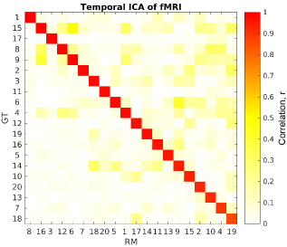
For the synthetic part of the data, we propose to simulate a $20\times 1334$ matrix of timecourses $\mathbf{y}$ by generating realistic autocorrelated samples that mimic observed fMRI timecourses to a good extent. Sampling 20 such timecourses that retain independence with respect to each other is challenging because independently sampled autocorrelated time series tend to be correlated with one another. Building on the simulation principles outlined in [43], we seek to avoid randomly correlated timecourses (sources) in order to prevent mismatches to the underlying ICA model we wish to test. In the same spirit, we also wish to have sources sampled from the same distribution used in the model, here a Laplace distribution. We developed the following steps in order to meet all these requirements:

Figure 5: Side-by-side comparison with the ground-truth (hybrid temporal ICA). The clear resemblance to the ground-truth maps suggests a successful recovery of the mixing matrix $\mathbf{A}$. The sample correlation $r$ is shown below each matched pair. Maps are sorted from highest to lowest correlation.

1)

Design a joint autocorrelation matrix $\mathbf{R}^{\mathbf{y}\mathbf{y}}$ for all sources. For the example above, this means a $\bar{C}N\times\bar{C}N$ block-diagonal correlation matrix ($\bar{C}N=26680$) with $\bar{C}$ blocks of size $N\times N$. Each block is designed with an exponentially decaying autocorrelation function such that the autocorrelation between timepoint $n$ and $n-1$ is in the order of 0.85, and between $n$ and $n-10$ is in the order of 0.2. This structure retains autocorrelation within each $N$-long section of an observation while retaining uncorrelation/independence among sections.

2)

Generate $50\mathrm{k}$ $\bar{C}N$-dimensional observations using a Gaussian copula [77] and the autocorrelation matrix $\mathbf{R}^{\mathbf{y}\mathbf{y}}$ from step 1. Using copulas enables transformation of the marginal distributions while retaining their correlation/dependence.

3)

For each of the $50\mathrm{k}$ copula-sampled observations, transform the sample into a Laplace distribution.

4)

For each of the $50\mathrm{k}$ transformed $\bar{C}N$-dimensional observations, reshape them into a $\bar{C}\times N$ matrix and compute the resulting $\bar{C}\times\bar{C}$ $\mathbf{R}^{\mathbf{y}}$ correlation matrix.

5)

Compute the median correlation matrix $\mathbf{R}_{med}^{\mathbf{y}}$ over the $50\mathrm{k}$ observed $\mathbf{R}^{\mathbf{y}}$.

6)

Retain the transformed observation whose $\mathbf{R}^{\mathbf{y}}$ is closest to $\mathbf{R}_{med}^{\mathbf{y}}$ and reject the rest.

This type of rejection sampling effectively produces the desired outcome. Finally, Gaussian noise is added to the mixture for a low $\mathrm{SNRdB}=3$. The condition number of $\mathbf{A}$ was 4.59.

In the results, the data was reduced using PRE and then processed with MISA to obtain independent timecourses. The correlation between ground-truth (GT) and PRE+MISA spatial map estimates (RM) is presented in Fig. 4, and the spatial maps (estimating $\mathbf{A}$ from $\hat{\mathbf{W}}^{-}$) in Fig. 5. MISI $=0.0365$.

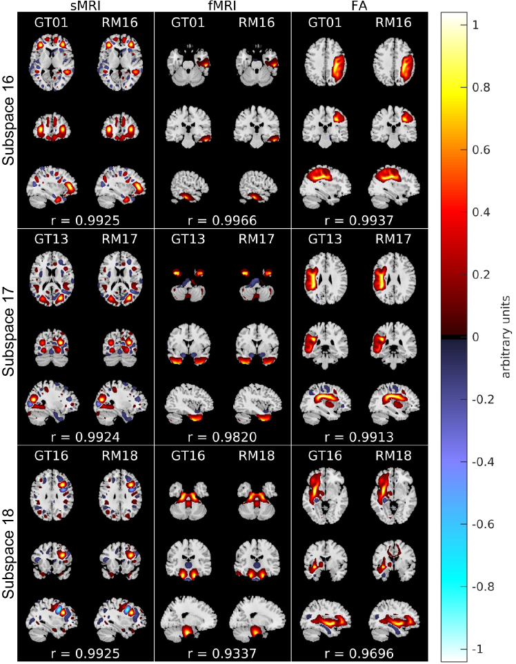
IV-C2 Multimodal IVA of sMRI, fMRI, and FA

In this multimodal fusion of structural MRI (sMRI), fMRI, and Fractional Anisotropy (FA) diffusion MRI data, the dimensionalities are $V_{1}=\mathrm{voxels}\approx 300\mathrm{k}$, $V_{2}=\mathrm{voxels}\approx 67\mathrm{k}$, $V_{3}=\mathrm{voxels}\approx 15\mathrm{k}$, respectively, and $N=\mathrm{subjects}=600$ (each modality measured on the same subject). We pursue a hybrid setting where only the mixing matrices $\mathbf{A}_{m}$ are taken from real datasets to overcome typically small $N$ in patient population studies. First, we let $C_{m}=20$ sources in each dataset. Then, $\mathbf{A}_{1}$, $\mathbf{A}_{2}$, and $\mathbf{A}_{3}$ must be $300\mathrm{k}\times 20$, $67\mathrm{k}\times 20$, and $15\mathrm{k}\times 20$, respectively. To each, we assign the first twenty aggregate 3D spatial maps published in [78], [76], [79], respectively.

(a) Structural MRI

(b) Functional MRI

(c) Fractional Anisotropy

Figure 6: Correlation with the ground-truth (multimodal IVA). The correlation between the spatial map estimates from MISA with PRE (RM) and the ground-truth (GT) is very high in all modalities, with little residual similarity across sources, suggesting the analysis was successful.

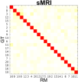
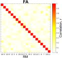
For the simulated part of the data, we generate three $20\times 600$ matrices of subject expression levels $\mathbf{y}$. $K=20$ subspaces, each with $d_{k}=3$ and $N=600$ observations, were sampled independently from a Gaussian copula, using an inverse exponential autocorrelation function with maximal correlation varying from $0.65$ to $0.85$ for each subspace. These were transformed to Laplace distribution marginals (not multivariate Laplace) so as to induce a controlled mismatch between the data (only SOS dependence) and the model subspace distributions (multivariate Laplace—all-order dependence). Finally, Gaussian noise was added separately in each dataset for a low $\mathrm{SNRdB}=3$. The condition numbers of $\mathbf{A}_{1}$, $\mathbf{A}_{2}$, and $\mathbf{A}_{3}$ were 1.52, 4.59, 1.63, respectively.

Figure 7: Summary of multimodal IVA maps. In each panel, ground-truth (GT) maps are presented on the left and maps estimated from MISA with PRE (RM) on the right. Each subspace represents the multimodal set of maps (joint features) with highest, median, and minimum correlation with the GT, from top to bottom, respectively. No IVA-L comparison available since it failed to converge, likely due to the small sample size ($N=600$).

In the results, the data was reduced using PRE and then processed with MISA to obtain independent subject expression levels. Per-modality correlation between ground-truth and PRE+MISA spatial maps are presented in Fig. 6, and spatial maps (estimating $\mathbf{A}$ from $\hat{\mathbf{W}}^{-}$) in Fig. 7. MISI $=0.0273$.

IV-C3 Multimodal MISA of fMRI, and EEG

We show the value of MDM models without data reduction for fusion of electroencephalography (EEG) event-related potentials (ERP) and fMRI datasets with dimensionality $V_{1}=\mathrm{time~{}points}\approx 600$, $V_{2}=\mathrm{voxels}\approx 67\mathrm{k}$, respectively, and $N=\mathrm{subjects}=1001$. Let $C_{1}=4$ and $C_{2}=6$ sources in the ERP and fMRI datasets, respectively, organized into $K=4$ subspaces ($y_{mi}$ represents source $i$ from dataset $m$):

$k=1$:

IVA-type, sources $y_{11}$ and $y_{21}$ ($d_{k}=2$);

$k=2$:

MISA-type, sources $y_{12}$, $y_{22}$ and $y_{23}$ ($d_{k}=3$);

$k=3$:

MISA-type, sources $y_{13}$, $y_{14}$ and $y_{24}$ ($d_{k}=3$);

$k=4$:

ISA-type, sources $y_{25}$ and $y_{26}$ ($d_{k}=2$).

Utilizing real spatial maps and timecourses, $\mathbf{A}_{1}$ and $\mathbf{A}_{2}$ must be $600\times 4$ and $67\mathrm{k}\times 6$, respectively, this time ensuring they form column-orthogonal mixings (with Gram-Schmidt).

For the simulated part of the data, we generate $4\times 1001$ and $6\times 1001$ matrices of subject expression levels for ERP and fMRI datasets, respectively. A total of $K=4$ $d_{k}$-dimensional subspaces with $N=600$ observations each were sampled from a multivariate Laplace distribution, using an inverse exponential autocorrelation function with maximal correlation of $0.65$ for each subspace. Noise was absent in both datasets. The condition number was 1.00 for both $\mathbf{A}_{1}$ and $\mathbf{A}_{2}$.

Fig. 8 shows the results obtained from constrained MISA-GP, i.e., with $\hat{\mathbf{A}}=\mathbf{W}^{\top}$ RE constraint using (10). No data reduction was performed on the data. The spatial fMRI maps and ERP timecourses were produced by estimating $\mathbf{A}$ from $\hat{\mathbf{W}}^{\top}$.

(a)

(b)

Figure 8: Multimodal MISA of fMRI and ERP. GT maps are presented on the left of each panel, MISA-GP estimates in the middle, and corrected MISA-GP estimates on the right. GT ERPs are presented in blue, MISA-GP ERPs in dashed red, and corrected MISA-GP ERPs in dashed cyan.

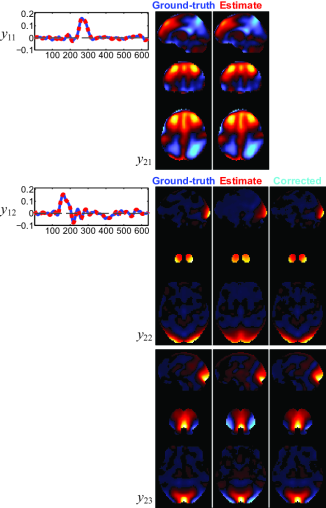
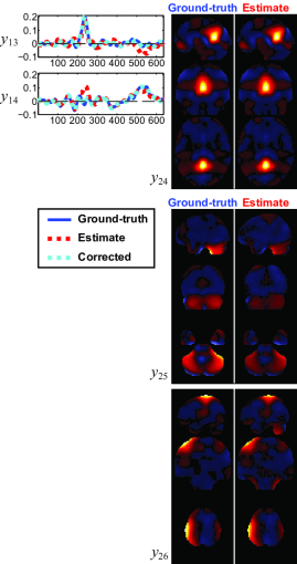
Since subspace independence is invariant to linear transformations (arbitrary basis) within any subspace [41], the estimation yields timecourses (red) and maps (middle) that do not match the GT exactly. In an attempt to correct for that, we performed additional within-modality ICAs on the columns of $\mathbf{A}_{m}$ corresponding to subspaces. This effectively selected for a particular basis within each subspace (right maps and cyan timecourses). The ability to choose a particular representation demonstrates the kinds of post-processing enabled by MDM models. Overall, this result validates and illustrates the benefit of a constrained optimization approach.

V Conclusion

We have presented MISA, an approach that solves multiple BSS problems (including ICA, IVA, ISA, and more) under the same framework, with remarkable performance and improved robustness even at low SNR. In particular, we derived a general formulation that controls for source scales, leveraging the flexible Kotz distribution in an interior point non-linear constraint optimization, with PRE as a general and flexible formulation for either direct subspace estimation or dimensionality reduction, in conjunction with combinatorial optimization for evasion of local minima, permitting self-correction to the closest subspace structures supported by the data (MISA-GP). Altogether, the proposed methods permit all-order statistics linkage across multidatasets as well as features of higher complexity to be identified and fully exploited in a direct, principled, and synergistic way, even at sample sizes as low as $N=600$. Flexible approaches like MISA are key to meet the growing complexity of multidataset tasks. These complexities are incorporated in the hybrid dataset standards we open source here, built from relevant results published in the brain imaging BSS literature. Generalizations building on this work could be easily developed exploring other divergence families. Future work will focus on compiling real multimodal datasets to validate MISA’s ability to capture reliable modes of shared and unique variability across and within modalities.

References

- [1] R. F. Silva, S. M. Plis, J. Sui, M. S. Pattichis, T. Adalı, and V. D. Calhoun, “Blind source separation for unimodal and multimodal brain networks: A unifying framework for subspace modeling,” IEEE J Sel Topics Signal Process, vol. 10, no. 7, pp. 1134–1149, 2016.
- [2] P. Comon and C. Jutten, Handbook of Blind Source Separation, 1st ed. Oxford, UK: Academic Press, 2010.
- [3] L. Yi, N. Dong, Y. Yun, B. Deng, D. Ren, S. Liu, and Y. Liang, “Chemometric methods in data processing of mass spectrometry-based metabolomics: A review,” Anal. Chim Acta, vol. 914, pp. 17–34, 2016.
- [4] S. Saito, K. Oishi, and T. Furukawa, “Convolutive Blind Source Separation Using an Iterative Least-Squares Algorithm for Non-Orthogonal Approximate Joint Diagonalization,” IEEE/ACM Trans Audio Speech Lang Process, vol. 23, no. 12, pp. 2434–2448, 2015.
- [5] A. A. Nielsen, “Multiset canonical correlations analysis and multispectral, truly multitemporal remote sensing data,” IEEE Trans Image Process, vol. 11, no. 3, pp. 293–305, 2002.
- [6] R. Ammanouil, A. Ferrari, C. Richard, and D. Mary, “Blind and Fully Constrained Unmixing of Hyperspectral Images,” IEEE Trans Image Process, vol. 23, no. 12, pp. 5510–5518, 2014.
- [7] V. D. Calhoun, J. Liu, and T. Adalı, “A review of group ICA for fMRI data and ICA for joint inference of imaging, genetic, and ERP data,” NeuroImage, vol. 45, no. 1, Supplement 1, pp. S163–S172, 2009.
- [8] V. D. Calhoun and J. Sui, “Multimodal fusion of brain imaging data: A key to finding the missing link(s) in complex mental illness,” Biol Psychiatry Cogn Neurosci Neuroimag, vol. 1, no. 3, pp. 230–244, 2016.
- [9] S. Bhinge, Y. Levin-Schwartz, and T. Adali, “Data-driven fusion of multi-camera video sequences: Application to abandoned object detection,” in Proc IEEE ICASSP 2017, 2017, pp. 1697–1701.
- [10] M. A. Nicolaou, V. Pavlovic, and M. Pantic, “Dyn. Probabilistic CCA Analysis of Affective Behavior and Fusion of Conts. Annotations,” IEEE Trans Pattern Anal Mach Intell, vol. 36, no. 7, pp. 1299–1311, 2014.
- [11] D. Lahat, T. Adalı, and C. Jutten, “Multimodal data fusion: An overview of methods, challenges, and prospects,” Proc IEEE, vol. 103, no. 9, pp. 1449–1477, 2015.
- [12] K. L. Miller, F. Alfaro-Almagro, N. K. Bangerter, D. L. Thomas, E. Yacoub, J. Xu, A. J. Bartsch, S. Jbabdi, S. N. Sotiropoulos, J. L. R. Andersson, L. Griffanti, G. Douaud, T. W. Okell, P. Weale, I. Dragonu, S. Garratt, S. Hudson, R. Collins, M. Jenkinson, P. M. Matthews, and S. M. Smith, “Multimodal population brain imaging in the UK Biobank prospective epidemiological study,” Nat Neurosci, vol. 19, no. 11, pp. 1523–1536, 2016.
- [13] V. D. Calhoun and T. Adalı, “Multisubject independent component analysis of fMRI: A decade of intrinsic networks, default mode, and neurodiagn. discovery,” IEEE Rev Biomed Eng, vol. 5, pp. 60–73, 2012.
- [14] A. Seghouane and A. Iqbal, “Sequential Dictionary Learning From Correlated Data: Application to fMRI Data Analysis,” IEEE Trans Image Process, vol. 26, no. 6, pp. 3002–3015, 2017.
- [15] A. R. Mohammadi-Nejad, G. A. Hossein-Zadeh, and H. Soltanian-Zadeh, “Structured and sparse canonical correlation analysis as a brain-wide multi-modal data fusion approach,” IEEE Trans Med Imaging, vol. 36, no. 7, pp. 1438–1448, 2017.
- [16] J.-H. Lee, T.-W. Lee, F. Jolesz, and S.-S. Yoo, “Independent vector analysis (IVA): Multivariate approach for fMRI group study,” NeuroImage, vol. 40, no. 1, pp. 86–109, 2008.
- [17] S. Bhinge, R. Mowakeaa, V. D. Calhoun, and T. Adalı, “Extraction of time-varying spatio-temporal networks using parameter-tuned constrained IVA,” IEEE Trans Med Imaging, 2019.
- [18] M. Pakravan and M. B. Shamsollahi, “Extraction and Automatic Grouping of Joint and Individual Sources in Multi-Subject fMRI Data Using Higher Order Cumulants,” IEEE J Biomed Health Inform, 2018.
- [19] M. Yu, K. A. Linn, P. A. Cook, M. L. Phillips, M. McInnis, M. Fava, M. H. Trivedi, M. M. Weissman, R. T. Shinohara, and Y. I. Sheline, “Statistical harmonization corrects site effects in functional connectivity measurements from multi-site fMRI data,” Hum Brain Mapp, vol. 39, no. 11, pp. 4213–4227, 2018.
- [20] H. Mirzaalian, L. Ning, P. Savadjiev, O. Pasternak, S. Bouix, O. Michailovich, G. Grant, C. Marx, R. Morey, L. Flashman, M. George, T. McAllister, N. Andaluz, L. Shutter, R. Coimbra, R. Zafonte, M. Coleman, M. Kubicki, C. Westin, M. Stein, M. Shenton, and Y. Rathi, “Inter-site and inter-scanner diffusion MRI data harmonization,” NeuroImage, vol. 135, pp. 311–323, 2016.
- [21] F. Alam, R. Mehmood, I. Katib, N. N. Albogami, and A. Albeshri, “Data Fusion and IoT for Smart Ubiquitous Environments: A Survey,” IEEE Access, vol. 5, pp. 9533–9554, 2017.
- [22] N. E. D. Elmadany, Y. He, and L. Guan, “Information Fusion for Human Action Recognition via Biset/Multiset Globality Locality Preserving Canonical Correlation Analysis,” IEEE Trans Image Process, vol. 27, no. 11, pp. 5275–5287, 2018.
- [23] M. Uzair, A. Mahmood, and A. Mian, “Hyperspectral Face Recognition With Spatiospectral Information Fusion and PLS Regression,” IEEE Trans Image Process, vol. 24, no. 3, pp. 1127–1137, 2015.
- [24] J. Yao, D. Meng, Q. Zhao, W. Cao, and Z. Xu, “Nonconvex-sparsity and Nonlocal-smoothness Based Blind Hyperspectral Unmixing,” IEEE Trans Image Process, 2019.
- [25] A. Villa, J. A. Benediktsson, J. Chanussot, and C. Jutten, “Hyperspectral Image Classification With Indep. Component Discriminant Analysis,” IEEE Trans Geosci Remote Sens, vol. 49, no. 12, pp. 4865–4876, 2011.
- [26] H. Xu, J. Zheng, A. Alavi, and R. Chellappa, “Cross-domain visual recognition via domain adaptive dictionary learning,” arXiv preprint, 2018. [Online]. Available: http://arxiv.org/abs/1804.04687
- [27] J. Fan, T. Zhao, Z. Kuang, Y. Zheng, J. Zhang, J. Yu, and J. Peng, “HD-MTL: Hierarchical Deep Multi-Task Learning Large-Scale Visual Recog.” IEEE Trans Image Process, vol. 26, no. 4, pp. 1923–1938, 2017.
- [28] H. Lu, C. Shen, Z. Cao, Y. Xiao, and A. van den Hengel, “An embarrassingly simple approach to visual domain adaptation,” IEEE Trans Image Process, vol. 27, no. 7, pp. 3403–3417, 2018.
- [29] M. Long, J. Wang, G. Ding, J. Sun, and P. S. Yu, “Transfer joint matching for unsupervised domain adaptation,” in Proc IEEE CVPR 2014, 2014, pp. 1410–1417.
- [30] V. M. Patel, R. Gopalan, R. Li, and R. Chellappa, “Visual domain adaptation: A survey of recent advances,” IEEE Signal Process Mag, vol. 32, no. 3, pp. 53–69, 2015.
- [31] Z. Cai, L. Wang, X. Peng, and Y. Qiao, “Multi-view super vector for action recognition,” in Proc IEEE CVPR 2014, 2014, pp. 596–603.
- [32] L. Tang, Z. Yang, and K. Jia, “Canonical Correlation Analysis Regularization: An Effective Deep Multi-View Learning Baseline for RGB-D Object Recognition,” IEEE Trans Cogn Devel Syst, 2018.
- [33] M. E. Sargin, Y. Yemez, E. Erzin, and A. M. Tekalp, “Audiovisual Synchronization and Fusion Using Canonical Correlation Analysis,” IEEE Trans Multimedia, vol. 9, no. 7, pp. 1396–1403, 2007.
- [34] L. Gao, R. Zhang, L. Qi, E. Chen, and L. Guan, “The Labeled Multiple Canonical Correlation Analysis for Information Fusion,” IEEE Trans Multimedia, vol. 21, no. 2, pp. 375–387, 2019.
- [35] P. Narvor, B. Rivet, and C. Jutten, “Audiovisual speech separation based on independent vector analysis using a visual voice activity detector,” in Proc LVA/ICA 2017, Grenoble, France, 2017, pp. 247–257.
- [36] F. Nesta, S. Mosayyebpour, Z. Koldovský, and K. Paleček, “Audio/video supervised independent vector analysis through multimodal pilot dependent components,” in Proc EUSIPCO 2017, 2017, pp. 1150–1164.
- [37] R. F. Silva, S. M. Plis, T. Adalı, and V. D. Calhoun, “Multidataset independent subspace analysis,” in Proc OHBM 2014, Hamburg, Germany, 2014, Poster 3506.
- [38] ——, “Multidataset independent subspace analysis extends independent vector analysis,” in Proc IEEE ICIP 2014, France, 2014, pp. 2864–2868.
- [39] R. F. Silva, S. M. Plis, M. S. Pattichis, T. Adalı, and V. D. Calhoun, “Incorporating second-order statistics in multidataset independent subspace analysis,” in Proc OHBM 2015, Honolulu, HI, 2015, Poster 3743.
- [40] P. Comon, “Independent component analysis, a new concept?” Signal Process, vol. 36, no. 3, pp. 287–314, 1994.
- [41] J.-F. Cardoso, “Multidimensional independent component analysis,” in Proc IEEE ICASSP 1998, vol. 4, Seattle, WA, 1998, pp. 1941–1944.
- [42] T. Kim, T. Eltoft, and T.-W. Lee, “Independent vector analysis: An extension of ICA to multivariate components,” in Proc ICA 2006, Charleston, SC, 2006, vol. 3889, pp. 165–172.
- [43] R. F. Silva, S. M. Plis, T. Adalı, and V. D. Calhoun, “A statistically motivated framework for simulation of stochastic data fusion models applied to multimodal neuroimaging,” NeuroImage, vol. 102, Part 1, pp. 92–117, 2014.
- [44] A. Bell and T. Sejnowski, “An information-maximization approach to blind separation and blind deconvolution.” Neural Comput, vol. 7, no. 6, pp. 1129–1159, 1995.
- [45] S.-I. Amari, “Natural gradient works efficiently in learning,” Neural Comput, vol. 10, no. 2, pp. 251–276, 1998.
- [46] M. Anderson, T. Adalı, and X. L. Li, “Joint blind source separation with multivariate gaussian model: Algorithms and performance analysis,” IEEE Trans Signal Process, vol. 60, no. 4, pp. 1672–1683, 2012.
- [47] D. Lahat, J. Cardoso, and H. Messer, “Second-order multidimensional ICA: Performance analysis,” IEEE Trans Signal Process, vol. 60, no. 9, pp. 4598–4610, 2012.
- [48] Q. V. Le, W. Y. Zou, S. Y. Yeung, and A. Y. Ng, “Learning hierarchical invariant spatio-temporal features for action recognition with independent subspace analysis,” in Proc CVPR 2011, 2011, pp. 3361–3368.
- [49] R. F. Silva and S. M. Plis, How to Integrate Data from Multiple Biological Layers in Mental Health? Springer, 2019, pp. 135–159.
- [50] A. Hyvärinen, J. Hurri, and P. Hoyer, Natural Image Statistics: A Probabilistic Approach to Early Computational Vision, 1st ed., ser. Computational Imaging and Vision. Springer, 2009, vol. 39.
- [51] T. Bouwmans, S. Javed, H. Zhang, Z. Lin, and R. Otazo, “On the Applications of Robust PCA in Image and Video Processing,” Proc IEEE, vol. 106, no. 8, pp. 1427–1457, 2018.
- [52] J. Pont-Tuset, P. Arbeláez, J. T. Barron, F. Marques, and J. Malik, “Multiscale combinatorial grouping for image segmentation and object proposal generation,” IEEE Trans Pattern Anal Mach Intell, vol. 39, no. 1, pp. 128–140, 2017.
- [53] N. Y. El-Zehiry and L. Grady, “Contrast driven elastica image segmnt.” IEEE Trans Image Process, vol. 25, no. 6, pp. 2508–2518, 2016.
- [54] Z. Szabó, B. Póczos, and A. Lőrincz, “Separation theorem for independent subspace analysis and its consequences,” Pattern Recognit, vol. 45, no. 4, pp. 1782–1791, 2012.
- [55] T.-W. Lee and T. J. Sejnowski, “Independent component analysis for mixed sub-gaussian and super-gaussian sources,” in Proc 4th JSNC. INC, 1997, pp. 132–139.
- [56] A. Hyvärinen and U. Köster, “FastISA: A fast fixed-point algorithm for independent subspace analysis,” in Proc ESANN, 2006, pp. 371–376.
- [57] M. Anderson, G.-S. Fu, R. Phlypo, and T. Adalı, “Independent vector analysis, the Kotz distribution, and performance bounds,” in Proc IEEE ICASSP 2013, Vancouver, Canada, 2013, pp. 3243–3247.
- [58] S. Kotz, “Multivariate distributions at a cross road,” in Proc NATO Advanced Study Institute, Statistical Distributions in Scientific Work. Calgary, Canada: Springer, 1974, pp. 247–270.
- [59] T. Eltoft, T. Kim, and T.-W. Lee, “Multivariate scale mixture of gaussians modeling,” in Proc ICA 2006, Charleston, USA, 2006, pp. 799–806.
- [60] M. Anderson, “Independent vector analysis: Theory, algorithms, and applications,” Doctoral Dissertation, University of Maryland, Baltimore County, Baltimore, NM, USA, 2013.
- [61] X. Li and T. Adali, “Independent component analysis by entropy bound minimization,” IEEE Transactions on Signal Processing, vol. 58, no. 10, pp. 5151–5164, 2010.
- [62] M. Anderson, X.-L. Li, and T. Adalı, “Nonorthogonal independent vector analysis using multivariate gaussian model,” in Proc LVA/ICA 2010, ser. Lecture Notes in Computer Science. France: Springer, 2010, vol. 6365, pp. 354–361.
- [63] D. Lahat and C. Jutten, “Joint independent subspace analysis using second-order statistics,” IEEE Trans Signal Process, vol. 64, no. 18, pp. 4891–4904, 2016.
- [64] S. Nadarajah, “The Kotz-type distribution with applications,” Statistics, vol. 37, no. 4, pp. 341–358, 2003.
- [65] J. F. Cardoso and B. H. Laheld, “Equivariant adaptive source separation,” IEEE Trans Signal Process, vol. 44, no. 12, pp. 3017–3030, 1996.
- [66] R. H. Byrd, P. Lu, J. Nocedal, and C. Zhu, “A limited memory algorithm for bound constrained optimization,” SIAM J Sci Comput, vol. 16, no. 5, pp. 1190–1208, 1995.
- [67] C. Zhu, R. H. Byrd, P. Lu, and J. Nocedal, “Algorithm 778: L-BFGS-B: Fortran subroutines for large-scale bound-constrained optimization,” ACM Trans Math Softw, vol. 23, no. 4, pp. 550–560, 1997.
- [68] J. Nocedal and S. Wright, Numerical Optimization, 2nd ed. New York, NY: Springer, 2006.
- [69] R. Waltz, J. Morales, J. Nocedal, and D. Orban, “An interior algorithm for nonlinear optimization that combines line search and trust region steps,” Math Prog, vol. 107, no. 3, pp. 391–408, 2006.
- [70] S. Haufe, F. Meinecke, K. Görgen, S. Dähne, J.-D. Haynes, B. Blankertz, and F. Bießmann, “On the interpretation of weight vectors of linear models in multivar. neuroimag.” NeuroImage, vol. 87, pp. 96–110, 2014.
- [71] Q. Le, A. Karpenko, J. Ngiam, and A. Ng, “ICA with reconstruction cost for efficient overcomplete feature learning,” in Proc NIPS 2011, Granada, Spain, 2011, pp. 1017–1025.
- [72] MIALAB, “Group ICA of fMRI Toolbox (GIFT),” 2015. [Online]. Available: http://trendscenter.org/trends/software/gift/index.html
- [73] S. Rachakonda, R. F. Silva, J. Liu, and V. D. Calhoun, “Memory efficient PCA methods for large group ICA,” Front Neurosci, vol. 10, p. 17, 2016.
- [74] S.-I. Amari, A. Cichocki, and H. H. Yang, “A new learning algorithm for blind signal separation,” Proc NIPS 1996, vol. 8, pp. 757–763, 1996.
- [75] O. Macchi and E. Moreau, “Self-adaptive source separation by direct or recursive networks,” in Proc ICDSP 1995, Cyprus, 1995, pp. 122–129.
- [76] E. A. Allen, E. B. Erhardt, E. Damaraju, W. Gruner, J. M. Segall, R. Silva, M. Havlicek, S. Rachakonda, J. Fries, R. Kalyanam, and et al., “A baseline for the multivariate comparison of resting-state networks,” Front Syst Neurosci, vol. 5, 2011.
- [77] R. Nelsen, An Introduction to Copulas, 2nd ed., ser. Springer Series in Statistics. New York, NY: Springer New York, 2006, vol. 1.
- [78] J. Segall, E. Allen, R. Jung, E. Erhardt, S. Arja, K. Kiehl, and V. Calhoun, “Correspondence between structure and function in the human brain at rest,” Front Neuroinform, vol. 6, p. 10, 2012.
- [79] L. Wu, V. D. Calhoun, R. E. Jung, and A. Caprihan, “Connectivity-based whole brain dual parcellation by group ICA reveals tract structures and decreased connectivity in schizophrenia,” Hum Brain Mapp, vol. 36, no. 11, pp. 4681–4701, 2015.