Asymptotically Optimal
Sampling-based Planners

1 Synonyms

AO planning, optimal motion planning

2 Definition

An asymptotically optimal sampling-based planner employs sampling to solve robot motion planning problems and returns paths with a cost that converges to the optimal solution cost, as the number of samples approaches infinity.

3 Overview

Sampling-based planners sample feasible robot configurations and connect them with valid paths. They are widely popular due to their simplicity, generality, and elegance in terms of analysis. They scale well to high-dimensional problems and rely only on well-understood primitives, such as collision checking and nearest neighbor data-structures. Roadmap planners, e.g., the Probabilistic Roadmap Method (PRM) (Kavraki et al 1996), construct a graph, where nodes are configurations and edges are local paths. The roadmap can be preprocessed and used to answer multiple queries. Alternatives, e.g., the Rapidly Exploring Random Tree (RRT) (LaValle and Kuffner Jr 2001), build a tree and aim to quickly explore the reachable configurations for solving a specific query. Tree-based variants can deal with challenges that involve significant dynamics, where there may not be access to a method (i.e., a steering function) for connecting two configurations with a local path.

Many early methods aimed to provide probabilistic completeness (Hsu et al 1999), i.e., a solution will be found, if one exists, as the number of sampled configurations approaches infinity. Further analysis focused on properties of configuration spaces, which allowed sampling to be effective, such as $\epsilon$-goodness (Kavraki et al 1998) and expansiveness (Hsu et al 1999). A large number of variants were proposed for enhancing the practical performance of sampling-based planning (Amato et al 1998; Kim et al 2003; Raveh et al 2011). These early methods did not focus on returning paths of high-quality. As the planners became increasingly faster, however, the focus transitioned towards understanding the conditions under sampling-based planners can asymptotically converge to paths that optimize a desirable cost function. This gave rise to a new family of sampling-based planners, which can also achieve asymptotic optimality.

Consider a robot in a workspace with obstacles, where a configuration $q$ is a vector of robot variables that define the workspace volume occupied by the robot.

Definition 1 (Configuration Space)

All possible configurations of the robot define a set $\mathcal{Q}\subset\mathbb{R}^{d}$. The feasible subset $\mathcal{Q}_{{\rm free}}\subseteq\mathcal{Q}$ and the infeasible subset $\mathcal{Q}_{{\rm obs}}\subseteq\mathcal{Q}$ refer to configurations that do not result or cause collisions with obstacles in the workspace, respectively.

The notion of collisions can be generalized to express any feasibility constraint.

Definition 2 (Feasible Paths with Strong $\delta$-clearance)

A feasible path $\sigma:[0,1]\rightarrow\mathcal{Q}_{{\rm free}}$ is a parameterized continuous curve of bounded variation. The set of all possible such paths is $\Sigma$. A feasible path $\sigma$ has strong $\delta$-clearance, if $\sigma$ lies entirely inside the $\delta$ interior of $\mathcal{Q}_{{\rm free}}$, i.e., $\forall\tau\in[0,1]:\sigma(\tau)\in int_{\delta}(\mathcal{Q}_{{\rm free}})$.

The $\delta$-clearance property guarantees there is always a $d$-dimensional $\delta$-ball in $\mathcal{Q}_{{\rm free}}$ - and, thus, a positive volume - around configurations of a solution path.

Definition 3 (Robustly Feasible Motion Planning)

Given $q_{\mathrm{init}}\subseteq\mathcal{Q}_{{\rm free}}$ and a set $\mathcal{Q}_{\mathrm{goal}}\subseteq\mathcal{Q}_{{\rm free}}$, the robustly feasible motion planning problem $(\mathcal{Q}_{{\rm free}},q_{\mathrm{init}},\mathcal{Q}_{\mathrm{goal}})$ asks for a feasible path $\sigma$ with strong $\delta$-clearance, so that $\sigma[0]=q_{\mathrm{init}}$ and $\sigma[1]\in\mathcal{Q}_{\mathrm{goal}}$.

Definition 4 (Optimal Motion Planning)

Given a path cost function $\mathtt{c}:\Sigma\rightarrow\mathbb{R}_{\geq 0}$, an optimal solution to the motion planning problem satisfies: $\sigma^{*}=\underset{\sigma}{\mathtt{argmin}}\ \mathtt{c}(\sigma)$.

The optimal solution need not be unique but the minimum cost is unique and finite. Let $\mathfrak{C}_{n}^{ALG}$ define the extended random variable corresponding to the cost of the minimum-cost solution returned by algorithm $ALG$ after $n$ iterations.

Definition 5 (Asymptotic Optimality)

An algorithm is asymptotically optimal if, for a robustly feasible motion planning problem $(\mathcal{Q}_{{\rm free}},q_{\mathrm{init}},\mathcal{Q}_{\mathrm{goal}})$, which admits a robustly optimal solution with finite cost $c^{*}=\mathtt{c}(\sigma^{*})$ ensures that:

$$P(\{\limsup_{n\rightarrow\infty}\ \mathfrak{C}_{n}^{ALG}=c^{*}\})=1.$$

The corresponding literature describes the guarantee of asymptotic optimality in terms of this event occurring asymptotically. This is highlighted in Fig 1.

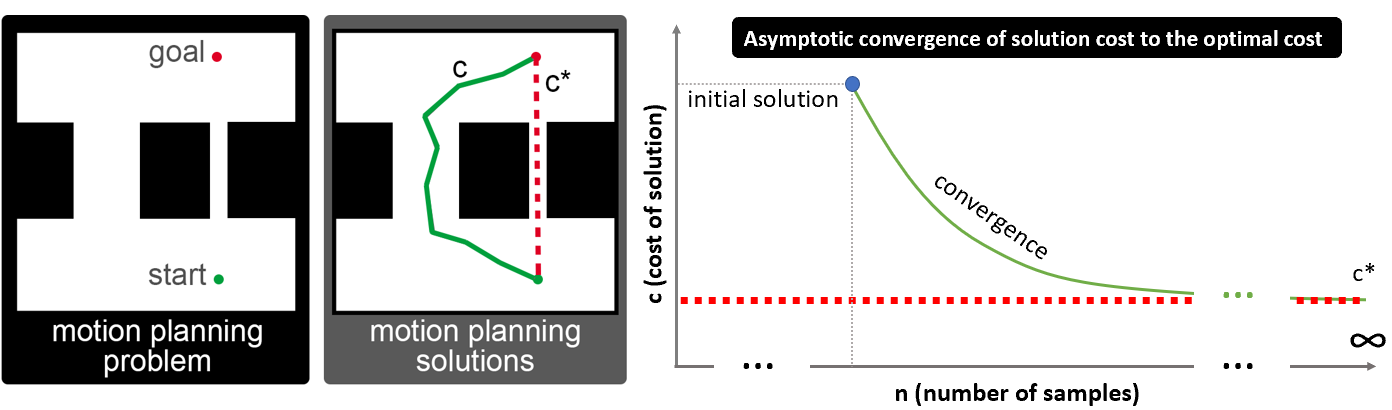
Figure 1: A motion planning problem (left) consists of the start, and goal in $\mathcal{Q}_{{\rm free}}$ (shown in white), while $\mathcal{Q}_{{\rm obs}}$ obstacles are black. A solution to the problem illustrated in the middle has a cost $c$ (green) relative to the optimal solution cost $c^{*}$ (red dashed). The plot on the right illustrates the asymptotic convergence of the solution cost $\mathtt{c}$ to the optimal one $\mathtt{c}^{*}$ over the number of samples $n$.

4 Key Research Findings

Table 1 summarizes different arguments for AO motion planning. Broadly, problems can be separated into kinematic ones where pairs of samples can be connected, and kinodynamic problems with non-trivial dynamics that do not allow such connections. Kinematic algorithms were proposed first, e.g., PRM^∗, RRT^∗ (Karaman and Frazzoli 2011), FMT^∗ (Janson et al 2015) and then AO kinodynamic methods were introduced, e.g., SST^∗ (Li et al 2016), AO-$\mathcal{A}$ (Hauser and Zhou 2016; Kleinbort et al 2020). The analyses also differ regarding the nature of the convergence property. Critical data-structures for these algorithms are also included in the table.

	Convergence	Structure	Algo	Condition
Kinematic	Almost sure	Roadmap	PRM*	$r_{n}\ >\ 2(1+\frac{1}{d})^{\frac{1}{d}}\Big{(}\frac{\mu(\mathcal{Q}_{{\rm free}})}{\zeta_{d}}\Big{)}^{\frac{1}{d}}\Big{(}\frac{\log n}{n}\Big{)}^{\frac{1}{d}}$ $k_{n}\ >\ e(1+\frac{1}{d})\log n$
	In probability	Search tree on Roadmap	FMT*	$r_{n}\ >\ 2(\frac{1}{d})^{\frac{1}{d}}\Big{(}\frac{\mu(\mathcal{Q}_{{\rm free}})}{\zeta_{d}}\Big{)}^{\frac{1}{d}}\Big{(}\frac{\log n}{n}\Big{)}^{\frac{1}{d}}$
	In probability	Tree with rewiring	RRT*	$r_{n}\ \geq\ (2+\theta)\Big{(}\frac{(1+\frac{\epsilon}{4})c^{*}}{(d+1)\theta(1-\nu)}\Big{)}^{\frac{1}{d+1}}$ $\Big{(}\frac{\mu(\mathcal{Q}_{{\rm free}})}{\zeta_{d}}\Big{)}^{\frac{1}{d+1}}\Big{(}\frac{\log n}{n}\Big{)}^{\frac{1}{d+1}}$
	Deterministic, dispersion-based	Roadmap	PRM*, FMT*	If sampling dispersion is $\mathcal{O}\Big{(}\Big{(}\frac{1}{n}\Big{)}^{\frac{1}{d}}\Big{)}$, then $r_{n}\in\omega\Big{(}\Big{(}\frac{1}{n}\Big{)}^{\frac{1}{d}}\Big{)}$
Kinodynamic	In probability	Forward search tree	SST*	Random selection, Monte Carlo Prop: random control and duration
	In probability	Forward search tree	AO-RRT	RRT selection in augmented state-cost space, Monte Carlo propagation
	In probability	Meta-algo	AO-$\mathcal{A}$	Repeatedly call a PC algorithm $\mathcal{A}$ with lowering cost-bound

Table 1: Summary of state-of-the-art results on asymptotic optimality. $r_{n}$ and $k_{n}$ describe the connection neighborhood for roadmaps as a radial region and number of nearest neighbors. $n$ is the number of samples, $d$ is the dimensionality of $\mathcal{Q}_{{\rm free}}$, $\mu$ is the volumetric measure, $\zeta_{d}$ is the volume of an unit $d$-dim. ball, $\epsilon\in(0,1)$ is the error from the optimum. For RRT^∗: $\theta\in(0,\frac{1}{4}),\nu\in(0,1)$. Kinodynamic planners do not require geometric neighborhood definitions.

For all methods employing random sampling, $\mathtt{c}_{n}$ is a random variable that depends on the realization of $n$ i.i.d samples. Consider an arbitrarily small error measure $\epsilon>0$. Then, failing to converge corresponds to $\mathtt{c}_{n}>(1+\epsilon)\mathtt{c}^{*}$. In terms of the type of convergence, ”almost sure convergence” dictates that out of all the realizations of the algorithm as $n$ reaches infinity, the failure event $\{\mathtt{c}_{n}>(1+\epsilon)\mathtt{c}^{*}\}$ is assured to occur a finite number of times, i.e., there exists a large enough $n_{0}\gg 1$ such that $\forall n>n_{0},\ \mathtt{c}_{n}\leq(1+\epsilon)\mathtt{c}^{*}$. ”Convergence in probability” only requires that at infinity the probability of the failure event goes to zero. Deterministic convergence can be argued geometrically given guarantees for the dispersion of samples. This means that the error is surely upper bounded by $\epsilon$ for a large enough $n$. These convergence results hold for all (arbitrarily small) values of $\epsilon$.

Analysis Model: Random Geometric Graphs

1 $\mathcal{G}(\mathcal{V}=\{q_{\mathrm{init}}\cup\mathcal{Q}_{\mathrm{goal}}\},\mathcal{E}=\emptyset)$;

2 for $n\ times$ do  $\mathcal{V}\leftarrow\mathcal{V}\cup{\mathtt{sample}()}$ ;

3 for ${v}\in\mathcal{V}$ do

4       for $u\in{\mathtt{Neighborhood}({v},\mathcal{G})}$ do

5             if $\mathtt{valid\_edge}(u,{v})$ then

6                   $\mathcal{E}\leftarrow\mathcal{E}\cup\{({v},u),(u,{v})\}$;

7                  

$\mathbf{return}\ {\mathtt{A^{*}}}(q_{\mathrm{init}},\mathcal{Q}_{\mathrm{goal}},\mathcal{G})$

Algo 1 PRM^∗ ($q_{\mathrm{init}},\mathcal{Q}_{\mathrm{goal}},n$)

1 $\mathcal{T}(\mathcal{V}=\{q_{\mathrm{init}}\},\mathcal{E}=\emptyset)$;

2 for $n\ times$ do

3       ${v}_{\mathrm{rand}}\leftarrow\mathtt{sample}()$;

4       $u_{\mathrm{near}}\leftarrow\mathtt{near}({v}_{\mathrm{rand}},\mathcal{T})$;

5       ${v}\leftarrow\mathtt{steer}(u_{\mathrm{near}},{v}_{\mathrm{rand}})$;

6       $\mathcal{N}\leftarrow\emptyset$;

7       for $u\in{\mathtt{Neighborhood}({v},\mathcal{T})}$ do

8             if $\mathtt{valid\_edge}(u,{v})$ then

9                   $\mathcal{N}\leftarrow\mathcal{N}\cup\{u\}$;

10                  

11      $u_{\mathrm{best}}\leftarrow\underset{u\in\mathcal{N}}{argmin}\ \mathtt{C}(u,\mathcal{T})+\mathtt{c}(\overrightarrow{u{v}})$;

12       $\mathcal{V}\leftarrow\mathcal{V}\cup\{{v}\}\ ;\ \mathcal{E}\leftarrow\mathcal{E}\cup\{(u_{\mathrm{best}},{v})\}$;

13       $\mathcal{T}\leftarrow\mathtt{rewire}({v},\mathcal{N},\mathcal{T})$;

14      

15$\mathbf{return}\ {\mathtt{trace}}(\mathcal{Q}_{\mathrm{goal}},\mathcal{T})$;

Algo 2 RRT^∗ ($q_{\mathrm{init}},\mathcal{Q}_{\mathrm{goal}},n$)

Identifying how sampling-based motion planners can achieve asymptotic optimality was first achieved by building on top of results in random geometric graphs . It resulted in new algorithms that provide this property, such as PRM^∗  and RRT^∗ (Karaman and Frazzoli 2011).

Outline of PRM^∗ and RRT^∗: Algo 1 describes PRM^∗: it resembles PRM except for the functional description of the neighborhood $\mathcal{N}$ in terms of $r_{n}$ or $k_{n}$ (Table 1). Algo 2 explains RRT^∗: the difference with RRT is a rewiring step that reasons about local connections between vertices within a neighborhood $\mathcal{N}$ given a radius $r_{n}$ (Table 1). Figure 2 shows that this radius heavily affects the solutions returned.

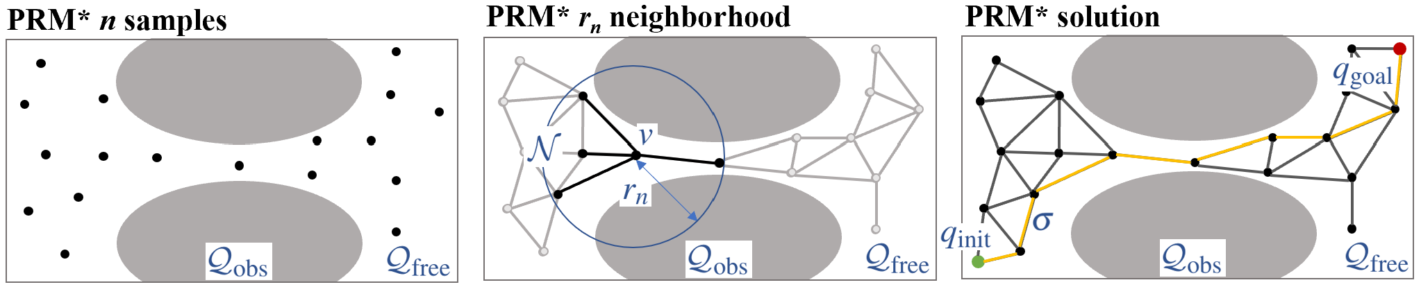
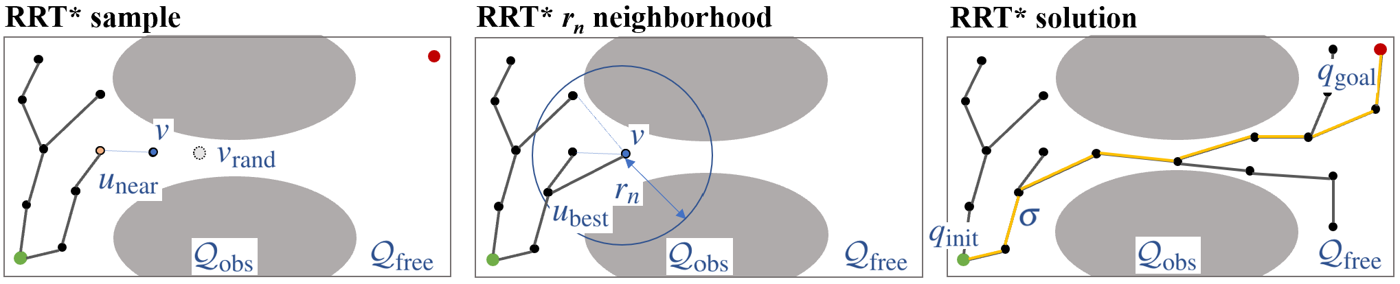
Figure 2: (Top): Different steps of PRM^∗: (Left) the $n$ random samples; (Middle) The $r_{n}$ neighborhood of each sample v is checked for a connection; (Right) The solution is traced over $\mathcal{G}$.
(Bottom): Different steps of RRT^∗: (Left) Dashed circles represent the random sample, the nearest node of the tree, and the result (blue point v) of steering towards the random sample; (Middle) The $r_{n}$ neighborhood of v is checked for the best connection; (Right) The solution is traced over $\mathcal{T}$.

These planners operate over underlying random geometric graphs. The graph theory literature describes properties of such graphs (Penrose 2003), including connectivity and percolation. $\mathcal{G}_{n}^{r}$ is surely connected when $r>\Big{(}\frac{1}{\zeta_{d}}\Big{)}^{\frac{1}{d}}{\Big{(}\frac{\log n}{n}\Big{)}}^{\frac{1}{d}}$. This threshold relates to AO requirements in motion planning as long as the graph is connected in the vicinity of the optimal path $\sigma^{*}$.

Definition 6 (Random Geometric Graph for Motion Planning)

The vertices of a random geometric graph $\mathcal{G}_{n}^{r}(\mathcal{V},\mathcal{E})$ correspond to $n$ i.i.d. uniformly sampled configurations in $\mathcal{Q}_{{\rm free}}$. Each vertex is connected with edges that lie in $\mathcal{Q}_{{\rm free}}$ to all configurations that are within a distance $r\in\mathbb{R}_{>0}$ away.

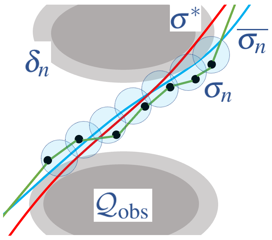
Figure 3: The optimal path $\sigma^{*}$ in red can touch the boundary of $\mathcal{Q}_{{\rm obs}}$. The clearance $\delta_{n}$ (light gray around the obstacles), and an observing path $\overline{\sigma}_{n}$ (in blue) can be studied by tiling $\overline{\sigma}_{n}$, i.e., defining a sequence of overlapping hyperballs. A solution $\sigma_{n}$ (in green) connects consecutive tiles.

Outline of the Analysis: Given the $\delta$-clearance of any feasible solution $\sigma_{n}$ (Definition 2), there exists a volume of $\mathcal{Q}_{{\rm free}}$ surrounding $\sigma_{n}$. Typically, the optimal path $\sigma^{*}$ itself can touch the $\mathcal{Q}_{{\rm free}}$ boundary and hence possesses 0-clearance at such contact points. As long as there exists a sequence of $\overline{\sigma}_{n}$ paths, each having $\delta_{n}$-clearance for $\delta_{n}>0$, such that $\lim\limits_{n\rightarrow\infty}\mathtt{c}(\overline{\sigma}_{n})=\mathtt{c}(\sigma^{*})$, the algorithm can operate over a positive volume around each $\overline{\sigma}_{n}$. This positive volume provides positive probability of sampling in these regions. The sequence of $\{\overline{\sigma}_{n}\}$ is called a sequence of observing paths. As $n$ increases, $\delta_{n}$, and $r_{n}$ decrease, meaning that $\delta_{n}$ expresses the algorithm’s ability to discover solutions through increasingly narrower corridors of $\mathcal{Q}_{{\rm free}}$.

Each $\overline{\sigma}$ has a volume of $\mathcal{Q}_{{\rm free}}$ given its clearance $\delta_{n}$. The volume surrounding an observing path $\overline{\sigma}$ is divided into a finite sequence of tiling constructions (hyperballs Karaman and Frazzoli (2011); Janson et al (2015), or hypercubes Solovey et al (2018)), where each tile has positive volume. By setting an appropriate $r_{n}$ value, the algorithm ensures connectivity in the $\delta_{n}$-clearance volume of each observing path $\overline{\sigma}_{n}$. This defines a solution path $\sigma_{n}$ along consecutively connected configurations along $\overline{\sigma}_{n}$. The k-near analysis broadly operates over the expected number of samples in the volumes described by the $r_{n}$ variants.

The probability of discovering a $\sigma_{n}$ close enough to a $\overline{\sigma}_{n}$, which in turn can get arbitrarily close to some desired $\sigma^{*}$ can be described in terms of the probability of sampling along the construction. At this stage, the functional estimate of $r_{n}$ depends on the nature of asymptotic convergence desired. This explains the difference between $r_{n}$ described by PRM^∗ for almost sure convergence, versus FMT^∗ (Janson et al 2015) described for convergence in probability. The latter analysis (Janson et al 2015) also deduced the convergence rate bound for PRM^∗ and FMT^∗ as $\mathcal{O}(n^{-\frac{1}{d+\rho}})$, when the algorithm is executed for $n$ samples in a $d$-dim. configuration space, where $\rho$ is an arbitrarily small constant. The convergence rate of AO sampling-based algorithms is an important factor, which dominates the finite time properties and practical performance of solutions.

Recent work (Solovey et al 2020) argues that tree-based AO sampling-based motion planners need to account for the existence of a chain of samples from the start along the hyperball tiling, for every hyperball, in addition to ensuring that the hyperball has a sample in it with increasing $n$. In a way, time is an additional dimension to deal with. This leads to an $r_{n}$ where the exponent changes to $\frac{1}{d+1}$ for RRT^∗ (Table 1).

Analysis Model: Batched and Deterministic Sampling

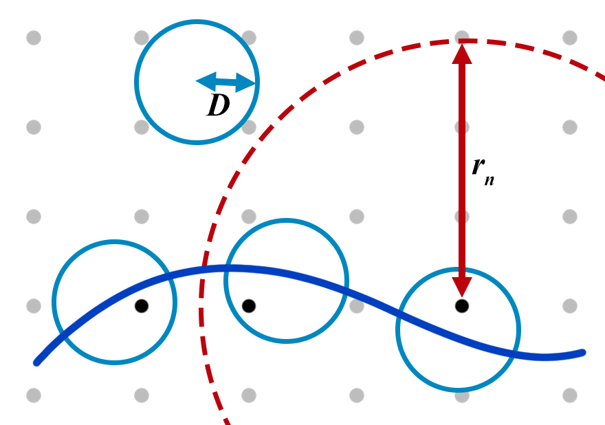
Figure 4: A deterministic sampling sequence with dispersion $D$, and tiling fo the path. The radius $r_{n}$ can be described in terms of $D$.

Low-dispersion deterministic sampling sequences guarantee samples with dispersion (Janson et al 2018) $D(\mathcal{V})=\mathcal{O}(n^{\frac{1}{d}})$, where $\mathcal{V}$ is the set of nodes of the planner. Dispersion is defined as the radius of the largest empty hyperball, which does not contain a sample. This is tighter than the expected dispersion from uniform sampling. As already mentioned, asymptotic guarantees are closely related to the ability to successfully sample within a sequence of tiling hyperballs along a path. With uniform sampling, the success of this event is probabilistic, and depends on the volume of the hyperballs in the sampling domain. If the dispersion of the determinstic sequence is guaranteed to be lower than the radius of the hyperball, a sample is assured inside the hyperball. Once samples are assured, the connection radius needs to only maintain connections between consecutive hyperballs. Results provide that an algorithm is AO if $\underset{{n\rightarrow\infty}}{\lim}\ D({v})\cdot r_{n}\rightarrow\infty$. The same line of work also expressed the connection radius bounds necessary for acceptable suboptimality error bounds, since such an error can express hyperball regions that admit such low-error solutions. It also provides a set of relations between dispersion and convergence rates as well as computational complexity results, including tighter bounds with $\epsilon$-net sampling (Tsao et al 2020).

Analysis Model: Monte Carlo Trees

A line of work focused on systems with dynamics and removed the requirement for a steering function by starting from first principles to achieve AO properties (Li et al 2016; Littlefield and Bekris 2018). The analysis starts with a Monte Carlo search tree, which performs random selection of nodes and random propagation of controls and does not depend on a steering function. Such an approach is shown to be AO, but also not practical due to slow convergence. A Best-Near variant of the Monte Carlo tree, however, was shown to be both asymptotically (near-)optimal and have practical convergence. The variant prioritizes the selection of nodes with good path quality within a neighborhood of the random sample and still uses Monte Carlo propagation. It can achieve AO properties by reducing the neighborhood size for this selection choice over computation time. The variant can be further improved in practice by sparsifying the underlying tree data structure and storing only nodes that locally have good path quality, giving rise to the SST algorithm (Fig  5). Heuristics can further speed up practical performance (Littlefield and Bekris 2018).

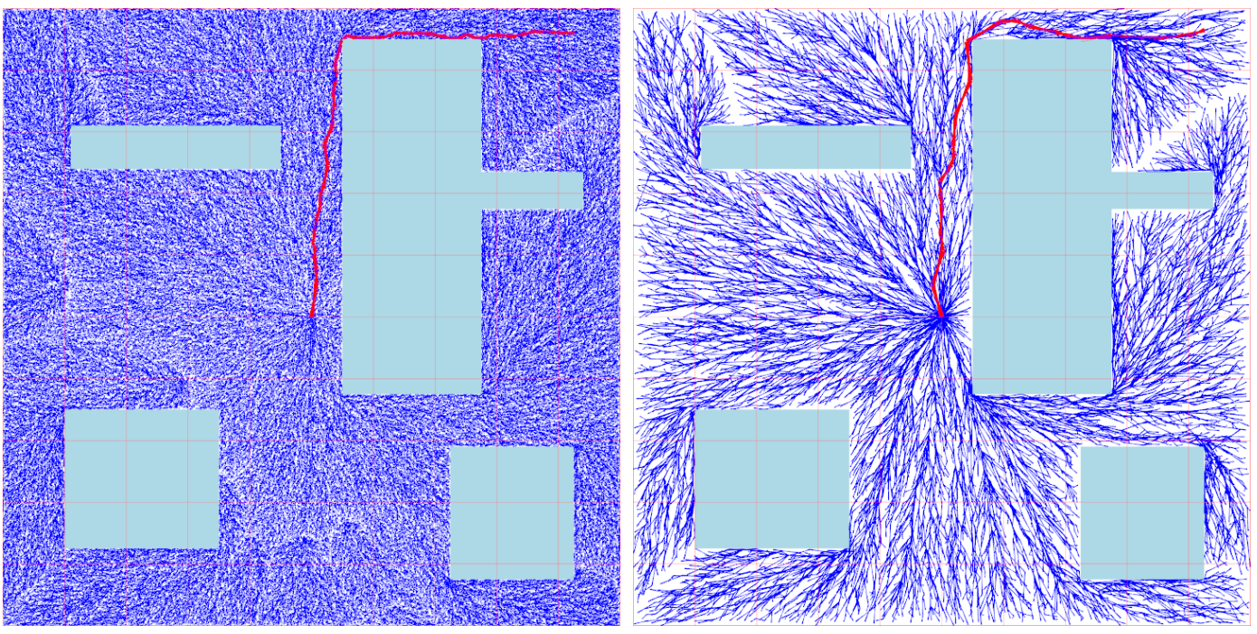
Figure 5: (Left): The SST approach propagates the node with the best path cost from the start in a neighborhood of a random sample to achieve asymp. near-optimality. For computational efficiency purposes, it also prunes nodes that are locally dominated in terms of path quality. (Right): A dense tree constructed using RRT^∗ (Algo 2) and then the sparser tree from SST (Li et al 2016).

The argument reasons about hyperballs along robust feasible paths, which are defined for some arbitrarily small $\epsilon$. The search tree has to discover a branch connecting consecutive hyperballs along the feasible path. Given an assumed smootheness in the dynamics, random controls and durations are sufficient to connect consecutive regions with probability measures independent of $n$. Then, it is sufficient to show that the algorithm can select every node infinitely often to allow opportunities to sample the desired edge using such Monte Carlo propagation. This process continues till the goal region is reached asymptotically.

Analysis Model: Search in State-Cost Space

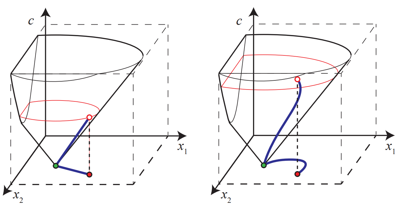
Figure 6: Two solutions in 2D $\{x_{1},x_{2}\}$ but with different costs, showing up as the difference in the state-cost space $\{x_{1},x_{2},c\}$ (Hauser and Zhou 2016).

Another direction for asymptotic optimality is a meta-algorithm, referred to as ${\tt AO}-\mathcal{A}$ (Hauser and Zhou 2016). The approach provides AO properties as long as a probabilistically complete (PC) algorithm $\mathcal{A}$, which achieves exponential convergence, is applied in the state-cost space. An algorithm is PC in the state-cost space if it is guaranteed to find a solution within a desired cost-bound, if one exists. The ${\tt AO}-\mathcal{A}$ algorithm inspects the state-cost space, and repeatedly calls algorithm $\mathcal{A}$ to produce a solution within the best cost bound discovered so far. Algorithm $\mathcal{A}$ takes the cost-bound as an argument and returns the first solution discovered within the input cost bound. By reducing the cost bound, the solution converges to the optimal cost. The PC and exponential convergence properties of $\mathcal{A}$ ensure that the expected running time is finite.

A kinodynamic AO-RRT  (Kleinbort et al 2020), which uses the virtues of randomness laid out in Monte-Carlo trees, but operates directly in the state-cost space for obtaining a solution with a single invocation of the algorithm was also studied. The selection procedure is the same as RRT in the state-cost space. The cost is instrumental is growing parts of the tree within the sampled cost bound. This ensures that as the cost of the best solution keeps decreasing, only the part of the search tree that can improve the solution is given a chance to grow using Monte-Carlo propagation. The argument formulates the probabilities of the tree traversing a construction of hyperballs as a Markov chain. The probability measures need to be shown to be independent of $n$. This simplified argument can then deduce that the random process reaches the sink-node of the chain asymptotically, i.e., it reaches the goal region following the sequence of regions along the construction.

Bridging Theoretical Guarantees and Practical Performance

Asymptotic optimality comes at the cost of computational overhead per iteration when compared to probabilistically complete or heuristic alternatives, which motivated work on balancing this desired property with practical performance.

Relaxed but Practical Guarantees: Computational trade-offs can be made by foregoing AO properties for asymptotic near-optimality(Marble and Bekris 2013). Such tradeoffs can utilize ideas from graph spanners, which refer to subgraphs that trade-off connectivity with bounded suboptimality. This trade-off is defined by a parameter that bounds the acceptable path cost degradation relative to the inclusion of edges during roadmap construction. The IRS algorithm is an incremental instantation of such a roadmap spanner approach, which only removes nodes. Extensions also remove nodes (Dobson and Bekris 2014) resulting in even smaller data structures, which offer benefits of computational and storage savings. Sparser variants of tree-based planners (Li et al 2016) also prune nodes that reach similar parts of $\mathcal{Q}$ with suboptimal paths.

This line of work has also looked on deciding the number of finite samples for a motion planner in practice by studying the finite time properties of AO methods (Dobson and Bekris 2013). This has yielded insights into the trade-offs of computation and solution quality expected from these algorithms. There have been additional models for studying near-optimality for tree-based approaches (Salzman and Halperin 2016) and those based on random geometric graphs (Solovey et al 2018; Solovey and Kleinbort 2020).

Improving Computational Efficiency: There are many ways to improve computational efficiency of AO planners, including through parallelizing (Bialkowski et al 2011) and caching collision checking (Bialkowski et al 2013). A way to speed up collision checking is to perform it lazily (Haghtalab et al 2018). Sampling strategies that focus on regions of $\mathcal{Q}_{{\rm free}}$ so as to improve existing solutions have been applied to both single-processor planners (Gammell et al 2015) and in parallel search processes with shared information (Otte and Correll 2013). Unlike RRT^∗, which uses local rewiring, global cost information propagation (Arslan and Tsiotras 2013) allows faster convergence in single-shot and replanning frameworks (Otte and Frazzoli 2016). Heuristics have also been incorporated into elements of kinodynamic planning (Littlefield and Bekris 2018). These optimizations can let AO algorithms quickly discover high-quality solutions, while improving on these solutions over time, i.e., they exhibit anytime behavior. Guidance can also arise out of human demonstrations, which guide an underlying AO search strategy (Bowen and Alterovitz 2016). On real-world systems, computation limits can be sidestepped by using a cloud system (Ichnowski and Alterovitz 2016; Bekris et al 2015). Hybrid approaches (Choudhury et al 2016) have combined optimization strategies to refine the solutions obtained in an AO framework.

AO Planners for Extensions of the Basic Problem

The progress in AO properties has allowed extending such guarantees to new domains. In particular, most of the above algorithms are applicable to kinematic domains given a Euclidean norm as an optimization objective. Below is a list of effort that extend analysis models to more complex problems.

Kinodynamic Planning: The kinodynamic case deals with motion planning for a robotic system with significant dynamics, i.e., the planning has to consider and account for velocities, accelerations (and other higher order dynamics). The approaches based on random geometric graphs assume the existence of a steering function to guarantee that two nearby configurations can be connected. In a kinodynamic problem, this does not always exist. An AO approach was proposed for systems with linearized dynamics (Webb and Van Den Berg 2013). Approaches leveraging newer analysis models of Monte Carlo trees (Li et al 2016; Littlefield and Bekris 2018), and search in the state-cost space (Hauser and Zhou 2016; Kleinbort et al 2020) have been proposed as AO algorithmic frameworks in the kinodynamic domain.

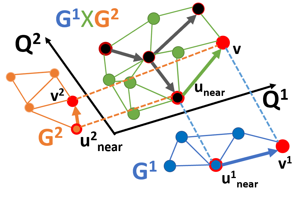
Figure 7: A tensor-roadmap $\mathcal{G}^{1}\times\mathcal{G}^{2}$ constructed from spaces $\mathcal{Q}^{1}$ and $\mathcal{Q}^{2}$. Black arrows denote the tree growing on the tensor roadmap. An extension to an adjacent vertex is demonstrated with $u_{\mathrm{near}}$ and ${v}$.

Multi-robot Motion Planning: The challenge in this case corresponds to the explosion in dimensionality. Centralized methods (Solovey et al 2014) have been argued to be AO (Shome et al 2019) under a sampling-based scheme that builds a graph in each robot’s $\mathcal{Q}_{{\rm free}}$ and searches online over an implicit representation of a tensor-roadmap of all the robots (shown in Fig. 7). The key idea is that the space of $r$ robots can be seen as the Cartesian product of the constituent spaces $\mathcal{Q}=\mathcal{Q}^{1}\times\mathcal{Q}^{2}\cdots\times\mathcal{Q}^{r}$. Accordingly, configurations and nodes can be split into the respective components in the constituent spaces. Fig 7 demonstrates the construction of AO roadmaps (ao_rm) in each space. The combination of these roadmaps has been shown to be AO in the entire $\mathcal{Q}$ and is called the tensor-roadmap : $\mathcal{G}=\mathcal{G}^{1}\times\mathcal{G}^{2}\cdots\times\mathcal{G}^{r}.$ Instead of explicitly creating and storing $\mathcal{G}$, the idea is to implicitly search it online through a tree $\mathcal{T}$ that is constructed over the nodes in $\mathcal{G}$. Avoiding storage and enumeration of the tensor-roadmap has important memory and computational benefits.

Motion Planning with Constraints: Many motion planning problems introduce constraints that force feasible solutions to lie on lower dimensional manifolds of $\mathcal{Q}$. Consider the difference between moving an arm versus moving it while keeping a grasped object upright. Such manifolds have 0-volume in the fully dimensional $\mathcal{Q}$. This complicates sampling processes. Approaches aim to ensure that samples and connections are found in such domains, while preserving theoretical properties (Kingston et al 2018). Some variants use projection operators to reach the constraint manifold, while others operate on tangent-spaces of the manifold by decomposing local neighborhoods into atlases (Jaillet and Porta 2013). A way to look at the problem is to decouple constraint satisfaction from the underlying planner (Kingston et al 2017). Such constraints also arise in integrated task and motion planning (Shome et al 2020; Vega-Brown and Roy 2016).

Domain	Algorithms
AO kinematic	PRM∗,RRT∗,RRG,RRT#, FMT∗,BIT∗,RRTX
AnO kinematic	IRS, SPARS, LBT-RRT
kinodynamic	SST∗,AO-$\mathcal{A}$,DIRT, AO-RRT
constraints	atlas-RRT∗
multi-robot	dRRT∗

Belief-space Planning: There are efforts in extending properties of sampling-based planners to belief-space planning (Agha-mohammadi et al 2012; Chaudhari et al 2013), where instead of planning over individual states, one has to reason about distributions. Recent work (Littlefield et al 2015) has also demonstrated the considerations and conditions under which such problems can be solved using AO algorithms that do not rely on steering functions.

5 Examples of Applications

There has been a push to ensure that methods for specific applications also afford AO guarantees. Some example domains (Fig 8) where AO motion planners have been proposed are the following: Self-driving cars (hwan Jeon et al 2013): AO planners have been applied to high-speed driving applications on car models with dymamics and fully integrated autonomy systems on shared roadways. Space robotics (Littlefield et al 2019): Space exploration involves deployment in highly unstructured environments. New emerging rovers, such as hybrid soft-rigid mechanisms based on tensegrity, introduce unique planning difficulties, which have been approached with AO planners. Planning for manipulators (Perez et al 2011; Schmitt et al 2017; Kimmel et al 2018; Shome and Bekris 2019): Planning for high-dimensional arms requires careful consideration of objects in the scene that need to be reached or avoided. Medical robotics (Patil et al 2015): Robustness and quality of solutions is important in medical tasks and promote AO considerations. Robot design (Baykal et al 2019): The design process for a robot can be seen as a model that, if optimized for a specific application, can significantly help in addressing challenging problems.

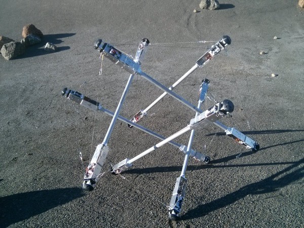
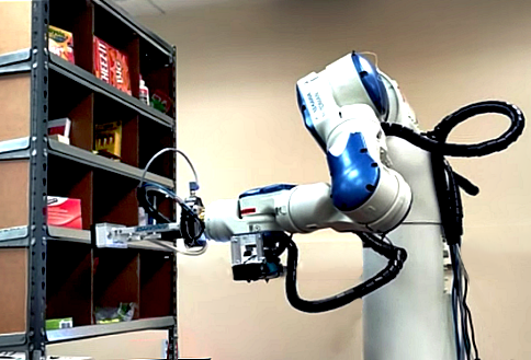
Figure 8: (Left to right): A car being planned for in simulation (Li et al 2016), a SUPERball rover for use in space exploration (Littlefield et al 2019), a manipulator planning to grasp objects inside a shelf (Kimmel et al 2018), and a simulation for multi-arm planning (Shome and Bekris 2019).

6 Future Direction for Research

Future research can help bridge the gap between theoretical properties and practical performance. For instance, most analyses of sampling-based planners reason for the worst-case. There is the potential for studying the expected behavior of these methods. The inspection of convergence rates as well as efficient data structures can provide insights regarding the practical and predictable deployment of AO methods.

Computing Platforms: There have been efforts to leverage modern computing hardware, such as parallelization (Bialkowski et al 2011) and custom chipsets (Murray et al 2016) to optimize queries and lead to significant speed-ups. Moreover, future planners will interact with cloud infrastructure and can share information (Bekris et al 2015; Ichnowski and Alterovitz 2016). GPUs, which have led to a revolution in machine learning, can also improve the efficiency of planners (Ichter et al 2017), given efficient parallel primitives (Pan and Manocha 2012).

Learning: Learning tools have been integrated with sampling-based planners to speed-up and improve performance of key components (Faust et al 2018). Learning how to perform sampling and identifying latent spaces of complex systems (Ichter and Pavone 2019) is an avenue for augmenting motion planners.

Planning under Uncertainty: Further analysis is needed to argue AO for motion planners in this domain (Littlefield et al 2015) as well as computational efficiency.

Integrated Task and Motion Planning: Many domains, such as manipulation, require identifying the sequence of planning problems to be addressed for solving a task. Recent progress has set the foundations for asymptotic optimality in this domain (Vega-Brown and Roy 2016) and provides opportunities for applying AO planners in problems, such as object rearrangement (Shome et al 2020).

References

- Agha-mohammadi et al (2012) Agha-mohammadi Aa, Chakravorty S, Amato NM (2012) On the probabilistic completeness of the sampling-based feedback motion planners in belief space. In: IEEE ICRA
- Amato et al (1998) Amato NM, Bayazit OB, Dale LK, Jones C, Vallejo D (1998) OBPRM: An obstacle-based PRM for 3d workspaces. In: WAFR
- Arslan and Tsiotras (2013) Arslan O, Tsiotras P (2013) Use of relaxation methods in sampling-based algorithms for optimal motion planning. In: IEEE ICRA
- Baykal et al (2019) Baykal C, Bowen C, Alterovitz R (2019) Asymptotically optimal kinematic design of robots using motion planning. Autonomous Robots 43(2):345–357
- Bekris et al (2015) Bekris K, Shome R, Krontiris A, Dobson A (2015) Cloud automation: Precomputing roadmaps for flexible manipulation. IEEE RAM 22(2):41–50
- Bialkowski et al (2011) Bialkowski J, Karaman S, Frazzoli E (2011) Massively parallelizing the RRT and the RRT*. In: IEEE/RSJ IROS
- Bialkowski et al (2013) Bialkowski J, Karaman S, Otte M, Frazzoli E (2013) Efficient collision checking in sampling-based motion planning. In: Algorithmic Foundations of Robotics X, Springer, pp 365–380
- Bowen and Alterovitz (2016) Bowen C, Alterovitz R (2016) Asymptotically optimal motion planning for tasks using learned virtual landmarks. IEEE RA-L 1(2):1036–1043
- Chaudhari et al (2013) Chaudhari P, Karaman S, Hsu D, Frazzoli E (2013) Sampling-based algorithms for continuous-time pomdps. In: 2013 American Control Conference, pp 4604–4610
- Choudhury et al (2016) Choudhury S, Gammell JD, Barfoot TD, Srinivasa SS, Scherer S (2016) Regionally accelerated batch informed trees (RABIT*): A framework to integrate local information into optimal path planning. In: IEEE ICRA, pp 4207–4214
- Dobson and Bekris (2013) Dobson A, Bekris KE (2013) A study on the finite-time near-optimality properties of sampling-based motion planners. In: IEEE/RSJ IROS, pp 1236–1241
- Dobson and Bekris (2014) Dobson A, Bekris KE (2014) Sparse roadmap spanners for asymptotically near-optimal motion planning. IJRR 33(1):18–47
- Faust et al (2018) Faust A, Oslund K, Ramirez O, Francis A, Tapia L, Fiser M, Davidson J (2018) PRM-RL: Long-range robotic navigation tasks by combining RL and sampling-based planning. In: IEEE ICRA, pp 5113–5120
- Gammell et al (2015) Gammell JD, Srinivasa SS, Barfoot TD (2015) Batch informed trees: Sampling-based optimal planning via the heuristically guided search of implicit random geometric graphs. In: IEEE ICRA
- Haghtalab et al (2018) Haghtalab N, Mackenzie S, Procaccia AD, Salzman O, Srinivasa SS (2018) The provable virtue of laziness in motion planning. In: 28th ICAPS
- Hauser and Zhou (2016) Hauser K, Zhou Y (2016) Asymptotically optimal planning by feasible kinodynamic planning in a state–cost space. IEEE T-Ro 32(6):1431–1443
- Hsu et al (1999) Hsu D, Latombe JC, Motwani R (1999) Path planning in expansive configuration spaces. International Journal of Computational Geometry & Applications 9(04n05):495–512
- Ichnowski and Alterovitz (2016) Ichnowski J, Alterovitz R (2016) Cloud based motion plan computation for power constrained robots. In: WAFR
- Ichter and Pavone (2019) Ichter B, Pavone M (2019) Robot motion planning in learned latent spaces. IEEE RA-L
- Ichter et al (2017) Ichter B, Schmerling E, Pavone M (2017) Group marching tree: Sampling-based approximately optimal motion planning on gpus. In: IEEE IRC, pp 219–226
- Jaillet and Porta (2013) Jaillet L, Porta JM (2013) Asymptotically-optimal path planning on manifolds. R:SS
- Janson et al (2015) Janson L, Schmerling E, Clark A, Pavone M (2015) Fast marching tree: A fast marching sampling-based method for optimal motion planning in many dimensions. IJRR 34(7):883–921
- Janson et al (2018) Janson L, Ichter B, Pavone M (2018) Deterministic sampling-based motion planning: Optimality, complexity, and performance. IJRR 37(1):46–61
- hwan Jeon et al (2013) hwan Jeon J, Cowlagi RV, Peters SC, Karaman S, Frazzoli E, Tsiotras P, Iagnemma K (2013) Optimal motion planning with the half-car dynamical model for autonomous high-speed driving. In: 2013 American Control Conference, IEEE, pp 188–193
- Karaman and Frazzoli (2011) Karaman S, Frazzoli E (2011) Sampling-based algorithms for optimal motion planning. IJRR 30(7):846–894
- Kavraki et al (1996) Kavraki LE, Svestka P, Latombe J, Overmars MH (1996) Probabilistic roadmaps for path planning in high-dimensional configuration spaces. IEEE TRA 12(4):566–580
- Kavraki et al (1998) Kavraki LE, Latombe JC, Motwani R, Raghavan P (1998) Randomized query processing in robot path planning. Journal of Computer and System Sciences 57(1):50–60
- Kim et al (2003) Kim J, Pearce RA, Amato NM (2003) Extracting optimal paths from roadmaps for motion planning. In: IEEE ICRA, vol 2, pp 2424–2429
- Kimmel et al (2018) Kimmel A, Shome R, Littlefield Z, Bekris K (2018) Fast, anytime motion planning for prehensile manipulation in clutter. In: IEEE-RAS Humanoids, pp 1–9
- Kingston et al (2017) Kingston Z, Moll M, Kavraki LE (2017) Decoupling constraints from sampling-based planners. In: ISRR
- Kingston et al (2018) Kingston Z, Moll M, Kavraki LE (2018) Sampling-based methods for motion planning with constraints. Annual review of control, robotics, and autonomous systems 1:159–185
- Kleinbort et al (2020) Kleinbort M, Granados E, Solovey K, Bonalli R, Bekris KE, Halperin D (2020) Refined Analysis of Asymptotically-Optimal Kinodynamic Planning in the State-Cost Space. IEEE ICRA
- LaValle and Kuffner Jr (2001) LaValle SM, Kuffner Jr JJ (2001) Randomized kinodynamic planning. IJRR 20(5):378–400
- Li et al (2016) Li Y, Littlefield Z, Bekris KE (2016) Asymptotically optimal sampling-based kinodynamic planning. IJRR 35(5):528–564
- Littlefield and Bekris (2018) Littlefield Z, Bekris KE (2018) Efficient and asymptotically optimal kinodynamic motion planning via dominance-informed regions. In: IEEE/RSJ IROS
- Littlefield et al (2015) Littlefield Z, Klimenko D, Kurniawati H, Bekris KE (2015) The importance of a suitable distance function in belief-space planning. In: ISRR
- Littlefield et al (2019) Littlefield Z, Surovik D, Vespignani M, Bruce J, Wang W, Bekris KE (2019) Kinodynamic planning for spherical tensegrity locomotion with effective gait primitives. IJRR
- Marble and Bekris (2013) Marble JD, Bekris KE (2013) Asymptotically near-optimal planning with probabilistic roadmap spanners. T-RO 29(2):432–444
- Murray et al (2016) Murray S, Floyd-Jones W, Qi Y, Sorin D, Konidaris G (2016) Robot planning on a chip. In: R:SS
- Otte and Correll (2013) Otte M, Correll N (2013) C-forest: Parallel shortest path planning with superlinear speedup. T-RO
- Otte and Frazzoli (2016) Otte M, Frazzoli E (2016) RRTX: Asymptotically optimal single-query sampling-based motion planning with quick replanning. IJRR 35(7):797–822
- Pan and Manocha (2012) Pan J, Manocha D (2012) Gpu-based parallel collision detection for fast motion planning. IJRR
- Patil et al (2015) Patil S, Pan J, Abbeel P, Goldberg K (2015) Planning curvature and torsion constrained ribbons in 3d with application to intracavitary brachytherapy. IEEE T-ASE 12(4):1332–1345
- Penrose (2003) Penrose M (2003) Random geometric graphs. 5, Oxford university press
- Perez et al (2011) Perez A, Karaman S, Shkolnik A, Frazzoli E, Teller S, Walter MR (2011) Asymptotically-optimal path planning for manipulation using incremental sampling-based algorithms. In: 2011 IEEE/RSJ IROS, pp 4307–4313
- Raveh et al (2011) Raveh B, Enosh A, Halperin D (2011) A little more, a lot better: Improving path quality by a path-merging algorithm. IEEE T-RO 27(2):365–371
- Salzman and Halperin (2016) Salzman O, Halperin D (2016) Asymptotically near-optimal RRT for fast, high-quality motion planning. IEEE T-RO 32(3):473–483
- Schmitt et al (2017) Schmitt PS, Neubauer W, Feiten W, Wurm KM, Wichert GV, Burgard W (2017) Optimal, sampling-based manipulation planning. In: IEEE ICRA, pp 3426–3432
- Shome and Bekris (2019) Shome R, Bekris KE (2019) Anytime multi-arm task and motion planning for pick-and-place of individual objects via handoffs. In: IEEE MRS
- Shome et al (2019) Shome R, Solovey K, Dobson A, Halperin D, Bekris KE (2019) dRRT*: Scalable and informed asymptotically-optimal multi-robot motion planning. Autonomous Robots pp 1–25
- Shome et al (2020) Shome R, Nakhimovich D, Bekris KE (2020) Pushing the boundaries of asymptotic optimality in integrated task and motion planning. In: WAFR
- Solovey and Kleinbort (2020) Solovey K, Kleinbort M (2020) The critical radius in sampling-based motion planning. IJRR
- Solovey et al (2014) Solovey K, Salzman O, Halperin D (2014) Finding a needle in an exponential haystack: Discrete RRT for exploration of implicit roadmaps in multi-robot motion planning. In: WAFR
- Solovey et al (2018) Solovey K, Salzman O, Halperin D (2018) New perspective on sampling-based motion planning via random geometric graphs. IJRR 37(10):1117–1133
- Solovey et al (2020) Solovey K, Janson L, Schmerling E, Frazzoli E, Pavone M (2020) Revisiting the asymptotic optimality of RRT∗. In: IEEE ICRA
- Tsao et al (2020) Tsao M, Solovey K, Pavone M (2020) Sample complexity of probabilistic roadmaps via epsilon-nets. IEEE ICRA
- Vega-Brown and Roy (2016) Vega-Brown W, Roy N (2016) Asymptotically optimal planning under piecewise-analytic constraints. In: WAFR
- Webb and Van Den Berg (2013) Webb DJ, Van Den Berg J (2013) Kinodynamic RRT*: Asymptotically optimal motion planning for robots with linear dynamics. In: IEEE ICRA