Observation and quantification of inertial effects on the drift of floating objects at the ocean surface

Abstract

We present results from an experiment designed to better understand the mechanism by which ocean currents and winds control flotsam drift. The experiment consisted in deploying in the Florida Current and subsequently satellite tracking specially designed drifting buoys of varied sizes, buoyancies, and shapes. We explain the differences in the trajectories described by the special drifters as a result of their inertia, primarily buoyancy, which constrains the ability of the drifters to adapt their velocities to instantaneous changes in the ocean current and wind that define the carrying flow field. Our explanation of the observed behavior follows from the application of a recently proposed Maxey–Riley theory for the motion of finite-size particles floating at the surface ocean. The nature of the carrying flow and the domain of validity of the theory are clarified, and a closure proposal is made to fully determine its parameters in terms of the carrying fluid system properties and inertial particle characteristics.

I Introduction

The assessment of motions of floating matter in the ocean is of importance for a number of key reasons. These range from improving search-and-rescue operations at sea Breivik et al. (2013); Bellomo et al. (2015); to better understanding the drift of flotsam of different nature including macroalgae such as Sargassum Gower and King (2008); Brooks, Coles, and Coles (2019); Wang et al. (2019), plastic litter Law et al. (2010); Cozar et al. (2014), airplane wreckage Trinanes et al. (2016); Miron et al. (2019), tsunami debris Rypina et al. (2013); Matthews et al. (2017), sea-ice pieces Szanyi, Lukovich, and Barber (2016), larvae Paris et al. (2020); Putman et al. (2016), and oil Olascoaga and Haller (2012); Gough et al. (2019); to better interpreting “Lagrangian” observations in the ocean Lumpkin and Pazos (2007); Beron-Vera, Olascoaga, and Lumpkin (2016). At present, largely piecemeal, ad-hoc approaches are taken to simulate the effects of ocean currents and winds on the drift of floating objects. A systematic approach ideally founded on first principles is needed. In an effort to contribute to building one, several experiments that involved the deployment and subsequent satellite tracking of specially designed drifting buoys of varied sizes, buoyancies, and shapes were carried out in the North Atlantic.

In this work we report results of the first experiment in the Florida Current. The drifters were deployed at once in coincidental position, off the southeastern coast of the Florida Peninsula. The differences in their trajectories are here explained as resulting from inertial effects, i.e., those due to the buoyancy and finite size of the drifters, which prevent them from instantaneously adjusting their velocities to changes in the carrying ocean current and wind fields. This is done by making use of a recently proposed framework for surface ocean inertial particle motion Beron-Vera, Olascoaga, and Miron (2019a), which is derived from the Maxey–Riley set Maxey and Riley (1983), the de-jure framework for the study of inertial particle dynamics in fluid mechanics Michaelides (1997); Provenzale (1999); Cartwright et al. (2010).

The standard Maxey–Riley set Maxey and Riley (1983) is a classical mechanics second Newton’s law that approximates the motion of inertial particles immersed in a fluid in motion. As such, it is given in the form of an ordinary differential equation, rather than a partial differential equation that would result from the exact formulation of the motion, which involves solving the Navier–Stokes equation with a moving boundary. The latter is a formidable task which would hardly provide as much insight as the analysis of an ordinary differential equation can provide.

The type of insight that analysis of the Maxey–Riley set can lead to includes foundation for realizing that the motion of neutrally buoyant particles should not synchronize with that of fluid particles, irrespective of how small Babiano et al. (2000); Vilela, de Moura, and Grebogi (2006); Sapsis and Haller (2008). Additional insight includes that which followed from earlier geophysical adaptions of the Maxey–Riley set, to wit, the possible role of mesoscale eddies as attractors of inertial particles Beron-Vera et al. (2015); Haller et al. (2016) and the tendency of the latter to develop large patches in the centers of the subtropical gyres Beron-Vera, Olascoaga, and Lumpkin (2016).

It is important to stress that the Maxey–Riley modeling framework for inertial particle motion on the ocean surface Beron-Vera, Olascoaga, and Miron (2019a) is quite different than the so-called leeway modeling approach of search-and-rescue applications at sea Breivik and Allen (2008). In such an approach, widely used for its simplicity Duhec et al. (2015); Trinanes et al. (2016); Allshouse et al. (2017), windage effects on objects are modeled by means of a velocity resulting from the addition of a small fraction of the wind field, established in an ad-hoc manner, to the surface ocean velocity

The rest of the paper is organized as follows. Section II describes the field experiment. The Maxey–Riley set for inertial ocean particle dynamics derived by Beron-Vera, Olascoaga, and Miron (2019a) is presented in Section III and clarified in Section IV with respect to the nature of the carrying flow, its domain of validity, and parameter specification. Section V describes the application of the Maxey–Riley framework to explain the behavior of each drifter type during the field experiment. Finally, Section VI offers a summary and the conclusions of the paper.

II The field experiment

The field experiment consisted in deploying simultaneously objects of varied sizes, buoyancies, and shapes on 7 December 2017 at (79.88^∘W, 25.74^∘N), situated off the southeastern Florida Peninsula in the Florida Current, and subsequently tracking them via satellite. These buoys will be referred to as special drifters to distinguish them from other more standardized drifter designs such as those from the Global Drifter Program (GDP). The special drifters were designed at the National Oceanic and Atmospheric Administration’s Atlantic Oceanographic and Meteorological Laboratory for this experiment.

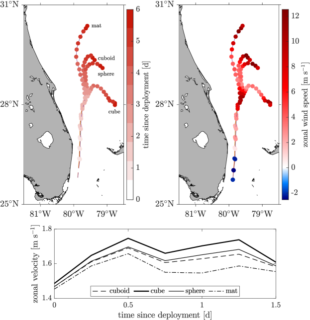
Figure 1: (top) Satellite-tracked trajectories of the special drifters with colors indicating time since deployment (left) and zonal (i.e., west-to-east) wind intensity (right). (bottom) Zonal velocity of the special drifters as a function of time from deployment to the instant when zonal wind speed reached its first peak.

Figure 2: (left) Trajectories of the special drifters (thin) and trajectories resulting from integrating a surface ocean current synthesis of altimetry-derived geostrophic flow, wind-induced Ekman drift, and drogued drifter velocities (dashed). (right) As in the left panel, but with dashed curves resulting from integrating leeway velocities constructed by adding to the altimetry/wind/drifter velocity synthesis small fractions (from top to bottom 1, 3, and 5%) of wind velocity.

Four types of special drifters were involved in the experiment. Three of them were comprised of a main body, made of Styrofoam, and a small, few-cm-long weighted drogue at the bottom to ensure that a SPOT^® trace Global Positioning System (GPS) tracker was maintained above the sea level. This tracker transmitted positions every 6 h. The main bodies of these special drifters represented a sphere of radius 12 cm, approximately, a cube of about 25 cm side, and a cuboid of approximate dimensions 30 cm $\times$ 30 cm $\times$ 10 cm. These special drifters were submerged below the sea level by roughly 10, 6.5, and 5 cm, respectively. The fourth special drifter, made of plastic, was designed to mimic a macroalgal mat, such as a Sargassum mat. The GPS tracker was collocated inside a small Styrofoam cone embedded in the mat. The maximal area spanned by the plastic mat was of about 250 cm $\times$ 50 cm and had a thickness of nearly 2 cm. It floated on the surface with the majority of its body slightly above the surface.

In this paper we focus on the analysis of the first week of trajectory records. There are two reasons for restricting to this period of time. First, the cube stopped transmitting position after one week. Thus extending the period of analysis beyond one week will shrink the space of parameters for exploration. Second, the special drifters tend to absorb water. This results in a change in their initial buoyancy over time and thus in their response to ocean current and wind drag. In the absence of empirical evidence, simulating this response will require one to propose some model for the time variation of the buoyancy, which we avoid to reduce uncertainties. With this in mind, we note that the special drifters were affected by a strong wind event that took place between 2 and 3 days after deployment (Fig. 1, top). This wind event unevenly impacted the trajectories, suggesting dominance of inertial effects. Furthermore, even prior to the anomalous wind event, the velocity of the special drifters was not uniform across them (Fig. 1, bottom), suggesting an uneven response of their motion to the ocean currents as well. This reinforces the idea that inertial effects dominated the motion of the special drifters.

Indeed, surface velocities alone cannot explain the different trajectories described by the special drifters, as is shown in the left panel of Fig. 2. The dashed curve in this figure is the trajectory that results from integrating a surface velocity representation starting from the deployment site and time. The thin curves are the various special drifter trajectories. The surface velocity corresponds to a synthesis of geostrophic flow derived from multisatellite altimetry measurements (Le Traon, Nadal, and Ducet, 1998) and Ekman drift induced by wind from reanalysis (Dee et al., 2011), combined to minimize differences with velocities of GDP drifters drogued at 15 m (Lumpkin and Pazos, 2007).

Moreover, a leeway velocity model is not capable of representing the variety of trajectories produced by the special drifters with a single windage strength choice. Several windage levels must be considered depending on the special drifter. This is insinuated in the right panel of Fig. 2, which shows (in dashed) trajectories resulting from integrating leeway velocities constructed by adding to the above surface velocity synthesis small fractions of the reanalyzed wind field involved in the synthesis. The windage levels are in the widely used ad-hoc range 1–5%. Duhec et al. (2015); Trinanes et al. (2016); Allshouse et al. (2017) Which level best suits a given special drifter cannot be assessed a priori. The Maxey–Riley theory of Beron-Vera, Olascoaga, and Miron (2019a) provides means for resolving this uncertainty by explicitly accounting for the effects of the inertia of the drifters on their motion.

III The Maxey–Riley framework

Consider a stack of two homogeneous fluid layers. The fluid in the bottom layer represents the ocean water and has density $\rho$. The top-layer fluid is much lighter, representing the air; its density is $\rho_{\mathrm{a}}\ll\rho$. Let $\mu$ and $\mu_{\mathrm{a}}$ stand for dynamic viscosities of water and air, respectively. The water and air velocities vary in horizontal position and time, and are denoted $v(x,t)$ and $v_{\mathrm{a}}(x,t)$, respectively, where $x=(x^{1},x^{2})$ denotes Cartesian position with $x^{1}$ (resp., $x^{2}$) pointing eastward (resp., northward) and $t$ is time. This configuration is susceptible to (Kelvin–Helmholtz) instability Le Blond and Mysak (1978), which is ignored assuming that the air–sea interface remains horizontal at all times. In other words, any wave-induced Stokes drift Phillips (1997) is accounted for implicitly by absorbing its effects in the water velocity $v$. Consider finally a solid spherical particle, of radius $a$ and density $\rho_{\mathrm{p}}$, floating at the air–sea interface. Define Beron-Vera, Olascoaga, and Miron (2019a)

$$\delta:=\frac{\rho}{\rho_{\mathrm{p}}}\geq 1.$$ (1)

Under certain conditions, clarified in Section IV.2, $\delta^{-1}$ approximates well the fraction of particle volume submerged in the water Beron-Vera, Olascoaga, and Lumpkin (2016); Beron-Vera, Olascoaga, and Miron (2019a). For future reference consider the following parameters depending on the inertial particle buoyancy $\delta$:

$$\Phi:=\frac{\mathrm{i}\sqrt{3}}{2}\left(\frac{1}{\varphi}-\varphi\right)-\frac{1}{2\varphi}-\frac{\varphi}{2}+1,$$ (2)

where

$$\varphi:=\sqrt[3]{\mathrm{i}\sqrt{1-(2\delta^{-1}-1)^{2}}+2\delta^{-1}-1}.$$ (3)

Nominally ranging in the interval $[0,2)$, $\Phi$ allows one to evaluate the height (resp., depth) of the emerged (resp., submerged) spherical cap as $\Phi a$ (resp., $(2-\Phi)a$).Beron-Vera, Olascoaga, and Miron (2019a) Finally,

$$\Psi:=\pi^{-1}\cos^{-1}(1-\Phi)-\pi^{-1}(1-\Phi)\sqrt{1-(1-\Phi)^{2}},$$ (4)

which nominally ranges in $[0,1)$ and gives the emerged (resp., submerged) particle’s projected (in the flow direction) area as $\pi\Psi a^{2}$ (resp., $\pi(1-\Psi)a^{2}$).Beron-Vera, Olascoaga, and Miron (2019a)

III.1 The full set

The Maxey–Riley set Maxey and Riley (1983); Gatignol (1983); Auton, Hunt, and Prud’homme (1988) includes several forcing terms that describe the motion of solid spherical particles immersed in the unsteady nonuniform flow of a homogeneous viscous fluid. These terms are the flow force exerted on the particle by the undisturbed fluid; the added mass force resulting from part of the fluid moving with the particle; and the drag force caused by the fluid viscosity.

Vertically integrating across the particle’s extent the Maxey–Riley set, enriched by further including the lift force Montabone (2002), which arises when the particle rotates as it moves in a (horizontally) sheared flow Auton (1987), and the Coriolis force Beron-Vera et al. (2015); Beron-Vera, Olascoaga, and Lumpkin (2016); Haller et al. (2016), which is the only perceptible effect of the planet’s rotation in the $x$-frame (as it has the local vertical sufficiently tilted toward the nearest pole to counterbalance the centrifugal force Gill (1982)), Beron-Vera et al. Beron-Vera, Olascoaga, and Miron (2019a) obtained the following Maxey–Riley set for surface ocean inertial particle motion:

$$\dot{v}_{\mathrm{p}}+\Big{(}f+\frac{1}{3}R\omega\Big{)}v_{\mathrm{p}}^{\perp}+\tau^{-1}v_{\mathrm{p}}=R\frac{\operatorname{D}\!{v}}{\operatorname{D}\!{t}}+R\Big{(}f+\frac{1}{3}\omega\Big{)}v^{\perp}+\tau^{-1}u,$$ (5)

where

$$u:=(1-\alpha)v+\alpha v_{\mathrm{a}}.$$ (6)

In (5) $v_{\mathrm{p}}$ is the velocity of the inertial particle and $\dot{v}_{\mathrm{p}}$ its acceleration; $f=f_{0}+\beta x^{2}$ is the Coriolis parameter; $\omega=-\nabla\cdot v^{\perp}=\partial_{1}v^{2}-\partial_{2}v^{1}$ is the (vertical component of the) water’s vorticity; $\smash{\frac{\operatorname{D}\!{}}{\operatorname{D}\!{t}}}v=\partial_{t}v+(\nabla v)v=\partial_{t}v+(\partial_{1}v)v^{1}+(\partial_{2}v)v^{2}$ is the total derivative of the water velocity along an ocean water particle trajectory; and parameters

$$R:=\frac{1-\frac{1}{2}\Phi}{1-\frac{1}{6}\Phi}\in[0,1),$$ (7)

and

$$\tau:=K\cdot\frac{1-\frac{1}{6}\Phi}{3\left(k^{-1}(1-\Psi)+\gamma k_{\mathrm{a}}^{-1}\Psi\right)\delta}\cdot\frac{a^{2}}{\mu/\rho}>0,$$ (8)

which measures the inertial response time of the medium to the particle. The nominal range of $\tau$ values is clarified in Section IV.2. In (8)

$$\gamma:=\frac{\mu_{\mathrm{a}}}{\mu}>0;$$ (9)

parameter $k>0$ (resp., $k_{\mathrm{a}}>0$) determines the projected length scale of the submerged (resp., emerged) inertial particle piece upon multiplication by the immersion (resp., emersion) depth (resp., height); and $0<K\leq 1$ is a correction factor that accounts for the effects of particle’s shape deviating from spherical, satisfying Ganser (1993)

$$K^{-1}=\frac{1}{3}\frac{a_{\mathrm{n}}}{a_{\mathrm{v}}}+\frac{2}{3}\frac{a_{\mathrm{s}}}{a_{\mathrm{v}}}.$$ (10)

Here $a_{\mathrm{n}}$, $a_{\mathrm{s}}$, and $a_{\mathrm{v}}$ are the radii of the sphere with equivalent projected area, surface area, and equivalent volume, respectively, whose average provide an appropriate choice for $a$. Finally, in (6)

$$\alpha:=\frac{\gamma k_{\mathrm{a}}^{-1}\Psi}{k^{-1}(1-\Psi)+\gamma k_{\mathrm{a}}^{-1}\Psi}.$$ (11)

Since $0\leq\alpha<1$, nominally, the convex combination (6) represents a weighted average of water and air velocities.

III.2 Slow manifold approximation

Set (5) represents a nonautonomous four-dimensional dynamical system in position ($x$) and velocity ($v_{\mathrm{p}}$). A two-dimensional system in $x$, which does not require specification of initial velocity for resolution, can be derived by noting that (5) is valid for sufficiently small particles or, equivalently, the inertial response time $\tau$ is short enough. More specifically, (5) involves both slow (position) and fast (velocity) variables, which makes it a singular perturbation problem. This enables one to apply geometric singular perturbation analysis Fenichel (1979); Jones (1995) extended to the nonautonomous case Haller and Sapsis (2008) to obtain Beron-Vera, Olascoaga, and Miron (2019a):

$$\dot{x}=v_{\mathrm{p}}=u+\tau u_{\tau}$$ (12)

$+\,O(\tau^{2})$ as $\tau\to 0$, where

$$u_{\tau}:=R\frac{\operatorname{D}\!{v}}{\operatorname{D}\!{t}}+R\Big{(}f+\frac{1}{3}\omega\Big{)}v^{\perp}-\frac{\operatorname{D}\!{u}}{\operatorname{D}\!{t}}-\Big{(}f+\frac{1}{3}R\omega\Big{)}u^{\perp}$$ (13)

with $\smash{\frac{\operatorname{D}\!{}}{\operatorname{D}\!{t}}}u$ being the total derivative of $u$, defined in (6), along a trajectory of $u$.

The reduced set (12) controls the evolution of the full set (5) on the manifold

$$M_{\tau}:=\{(x,v_{\mathrm{p}},t):v_{\mathrm{p}}=u(x,t)+\tau u_{\tau}(x,t)\},$$ (14)

which is referred to as a slow manifold because (5) restricted to $M_{\tau}$, i.e., (12), represents a slowly varying system (Fig. 3). Invariant up to trajectories leaving it through its boundary, and unique up to an error of $O(\mathrm{e}^{-1/\tau})\ll O(\tau)$,Fenichel (1979) $M_{\tau}$ normally attracts all solutions of the $\tau\to 0$ limit of (5) exponentially fast. The only caveat Haller and Sapsis (2008) is that rapid changes in the carrying flow velocity, represented by $u$, can turn the exponentially dominated convergence of solutions on $M_{\tau}$ not necessarily monotonic over finite time.

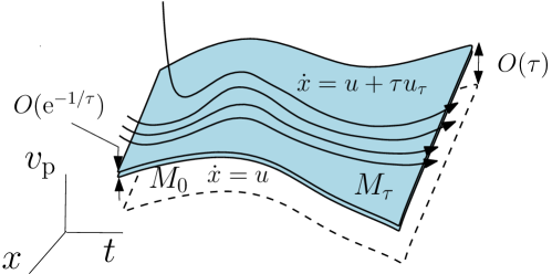
Figure 3: Geometry of the Maxey–Riley set (5) dynamics in the extended phase space. Unique up to an error of $O(\mathrm{e}^{-1/\tau})\ll O(\tau)$, the locally invariant slow manifold $M_{\tau}$ (14) normally attracts all solutions of the Maxey–Riley set when $\tau>0$ is small exponentially fast. This lies $O(\tau)$-close to the critical manifold $M_{0}$. For the fast dynamics, i.e., with $t$ rescaled by $\tau^{-1}$, $M_{0}$ is filled with fixed points, while for the slow dynamics, i.e., with $t$ unscaled, motion on $M_{0}$ is nontrivial, evolving according to the buoyancy-weighted average of water and air velocities $u$ (6). Yet motion off $M_{0}$ is not controlled by the dynamics on it.

IV Clarification of the Maxey–Riley set

IV.1 Critical manifold

The $\tau=0$ limit of (5) with $t$ rescaled by $\tau^{-1}$ to form a fast timescale has a large set of fixed points, which, given by $v_{\mathrm{p}}=u$, entirely fill $M_{0}$, called the critical manifold. Motion on $M_{0}$ is thus trivial for the $\tau=0$ limit of the fast form of (5). The $\tau=0$ limit of the slow form of (5), i.e., with $t$ unscaled, blows this motion up to produce nontrivial behavior on $M_{0}$, yet leaving the motion undetermined off $M_{0}$, which is controlled by $M_{\tau}$ when $\tau>0$ small.

The idea that motion on $M_{0}$ is trivial Jones (1995) must be understood in the specific dynamical systems sense above and should not be confused with implying that $\dot{x}=u$ cannot support rich dynamics. Clearly, rich dynamics can even be supported by the carrying velocity in the original Maxey–Riley model setting with a single fluid and a finite-size particle either heavier or lighter than the fluid. Yet in that case the interest lies in the potentially much richer dynamics Cartwright et al. (2010) that inertial effects may produce. The situation is different in the present case, wherein the carrying flow ($u$) depends on the buoyancy of the particle, cf. (6), and thus has inertial effects built in. Indeed, $u$ is not given a priori as in the standard fluid mechanics setting Cartwright et al. (2010). Rather, it follows from vertically integrating the drag force (Beron-Vera, Olascoaga, and Miron, 2019a). In other words, inertial effects are felt by the particle even when $\tau=0$. It turns out, as we will show below, that $\dot{x}=$u describes the trajectories of the special drifters over the period analyzed reasonably well.

It is important to realize that $\dot{x}=u$ is quite different than the so-called leeway model, i.e., one of the form $\dot{x}=v+\varepsilon v_{\mathrm{a}}$ where $\varepsilon>0$ is small. The leeway factor $\varepsilon$ is, as noted above, commonly chosen in an ad-hoc manner to reduce differences with observations Duhec et al. (2015); Trinanes et al. (2016); Allshouse et al. (2017). Yet buoyancy-dependent models for $\varepsilon$ have been proposed in the literature Röhrs et al. (2012); Nesterov (2018). But at odds with the Maxey–Riley approach, these models are obtained by neglecting inertia and assuming an exact cancellation between water and air drag forces.

Clearly, one should not expect that the leading-order contribution to the reduced Maxey–Riley set (12) be sufficient to describe all aspects of inertial particle motion in the ocean. Examples of relevant aspects include clustering at the center of the subtropical gyres Beron-Vera, Olascoaga, and Lumpkin (2016); Beron-Vera, Olascoaga, and Miron (2019a), phenomenon supported on measurements of plastic debris concentration Cozar et al. (2014) and the analysis of undrogued drifter trajectories Beron-Vera, Olascoaga, and Lumpkin (2016); Beron-Vera, Olascoaga, and Miron (2019a), or the role of mesoscale eddies as attractors or repellers of inertial particles depending on the polarity of the eddies and the buoyancy of the particles Beron-Vera et al. (2015); Haller et al. (2016); Beron-Vera, Olascoaga, and Miron (2019a) despite the Lagrangian resilience of their boundaries Beron-Vera et al. (2013); Haller and Beron-Vera (2013); Beron-Vera et al. (2018a, b), which is also backed on observations van der Mheen, Pattiaratchi, and van Sebille (2019). The cited phenomena, which act on quite different timescales, all require both $O(1)$ and $O(\tau)$ terms in (12) for their description Beron-Vera et al. (2015); Haller et al. (2016); Beron-Vera, Olascoaga, and Lumpkin (2016); Beron-Vera, Olascoaga, and Miron (2019a) consistent with the slow manifold $M_{\tau}$ in (14), rather than the critical $M_{0}$, controlling the time-asymptotic dynamics of the $\tau\to 0$ limit of the Maxey–Riley set (5).

IV.2 Domain of validity

Unlike stated in Beron-Vera, Olascoaga, and Miron (2019a), the domain of applicability of the Maxey–Riley set is not extensible to all possible $\delta$ values, which nominally range in a very large interval bounded by 1 from below. Indeed, the fraction of submerged particle volumeBeron-Vera, Olascoaga, and Miron (2019a)

$$\sigma=\frac{1-\delta_{\mathrm{a}}}{\delta-\delta_{\mathrm{a}}},$$ (15)

where

$$1\leq\delta\leq\frac{\rho}{\rho_{\mathrm{a}}}\gg 1,\quad\frac{\rho_{\mathrm{a}}}{\rho}\leq\delta_{\mathrm{a}}:=\frac{\rho_{\mathrm{a}}}{\rho_{\mathrm{p}}}\leq 1,$$ (16)

as static stability (Archimedes’ principle) demands, so $0\leq\sigma\leq 1$. Note that $\rho\gg\rho_{\mathrm{a}}$ implies $\delta\gg\delta_{\mathrm{a}}$ and as a result $\sigma\approx(1-\delta_{\mathrm{a}})/\delta$, which may be further approximated by $\delta^{-1}$ if $\delta_{\mathrm{a}}\ll 1$. The latter does not follow from $\rho\ll\rho_{\mathrm{a}}$ as incorrectly stated in Beron-Vera, Olascoaga, and Miron (2019a). It is an assumption which holds provided that $\delta$ is not too large. This follows from noting that $\delta_{\mathrm{a}}\equiv(\rho_{\mathrm{a}}/\rho)\cdot\delta$. Thus inferences made in Beron-Vera, Olascoaga, and Miron (2019a) on behavior as $\delta\to\infty$ are not formally correct and should be ignored. In particular, Section IV.B of Beron-Vera, Olascoaga, and Miron (2019a) should be omitted, and the left and middle panels of Fig. 2 in that paper, which shows $\alpha$ as a function of $\delta$ over a large range, should be interpreted with the above clarification in mind. Also, the formal ranges of parameters $\Phi$, $\Psi$, and $R$ are smaller than their nominal ones (stated above).

Currently underway Beron-Vera, Olascoaga, and Miron (2019b) is a corrigendum and addendum to Beron-Vera, Olascoaga, and Miron (2019a) where it is shown that the correct way to formulate the Maxey–Riley set so it is valid for all possible buoyancy values is by using, instead of $\delta$, the exact fraction of submerged volume $\sigma$, as given in (15). In Beron-Vera, Olascoaga, and Miron (2019b) it is shown, for instance, that the $\sigma\to 0$ (equivalently, $\delta\to\infty$) limit is symmetric with respect to the $\sigma\to 1$ (equivalently, $\delta\to 1$) limit, as it can be expected. Also, additional terms, involving air quantities must be included, both in the full and reduced sets if $\delta$ is allowed to take values in its full nominal range. It is important to note, however, that for the purposes of the present work, which involves dealing with observed $\delta$ values not exceeding $4$ or so, these additional terms can be safely neglected and thus is appropriate to use sets (5) or (12) as presented above.

IV.3 Parameter specification

In order for the Maxey–Riley parameters to be fully determined by the carrying fluid system properties and the inertial particle’s characteristics, the projected length factors, $k$ and $k_{\mathrm{a}}$, must first be specified. These should depend on how much the sphere is exposed to the air or immersed in the water to account for the effect of the air–sea interface (boundary) on the determination of the drag. With this in mind, we make the following proposition:

$$k=k_{\mathrm{a}}=\delta^{-r},\quad r>0.$$ (17)

Making $k=k_{\mathrm{a}}$ guarantees the leeway factor $\alpha$ in (11) to grow with $\delta$. This assures the air component of the carrying flow field to dominate over the water component as the particle gets exposed to the air. This is consistent with making $k=k_{\mathrm{a}}$ to decay with $\delta$ as this guarantees the inertial response time $\tau$ in (8) to shorten as the particle gets exposed to the air. Indeed, ignoring boundary effects, for a spherical particle that is completely immersed in the water $\tau=a^{2}\rho/3\mu$,Sapsis and Haller (2008); Beron-Vera, Olascoaga, and Miron (2019a) while $\tau=a^{2}\rho_{\mathrm{a}}/3\mu_{\mathrm{a}}\equiv(\rho_{\mathrm{a}}/\rho\gamma)\cdot(a^{2}\rho/3\mu)$ if the particle is fully exposed to the air. Using mean density values $\rho=1025$ $\mathrm{k}\mathrm{g}\,\mathrm{m}^{-3}$ and $\rho_{\mathrm{a}}=1.2$ $\mathrm{k}\mathrm{g}\,\mathrm{m}^{-3}$, and mean dynamic viscosity values $\mu=0.001$ $\mathrm{k}\mathrm{g}\,\mathrm{m}^{-1}\mathrm{s}^{-1}$ and $\mu_{\mathrm{a}}=1.8\times 10^{-5}$ $\mathrm{k}\mathrm{g}\,\mathrm{m}^{-1}\mathrm{s}^{-1}$, the lower bound on $\tau$ is approximately $0.05\cdot(a^{2}\rho/3\mu)$. Clearly, with $k=k_{\mathrm{a}}$ depending on $\delta$ as in (17), $\lim_{\delta\to\infty}\tau=0$. But this limit, as clarified above, is outside the domain of validity of the Maxey–Riley set (5) or its reduced form (12). It turns out that what really matters once the theory is confronted with observations is that (17) makes $\tau$ to decay at a faster rate with increasing $\delta$ than $k=k_{\mathrm{a}}=1$, which corresponds to setting the projected length of the submerged (resp., emerged) particle piece to be equal to the submerged depth (resp., emerged height). In fact, below we show that $r\approx 3$ best fits observations. In Beron-Vera, Olascoaga, and Miron (2019b) we will report on results aimed at providing a stronger foundation for (17) based on direct numerical simulations of low-Reynolds-number flow around an spherical cap of different heights. To the best of our knowledge, a drag coefficient formula for this specific setup is lacking. An important aspect that these simulations, in progress at the time of writing, will account for is the effect of the boundary on which the spherical cap rests on, which may lead to changes to the bounds on $\tau$ noted above.

V Using the Maxey–Riley framework to explain the behavior of the special drifters

Table 1 presents our estimates for the parameters that characterize the special drifters as inertial particles evolving according to the Maxey–Riley set, in its full (5) or reduced (12) version. These are classified into primary parameters ($a$, $K$, and $\delta$) and secondary parameters ($\alpha$, $R$, and $\tau$), which derive from the primary parameters.

The radius $a$ and shape correction factor $K$ follow from each special drifter’s dimension and shape specification. In computing the buoyancy $\delta$ we relied on the estimate of the immersion depth ($h$) for each special drifter at the Rosenstiel School of Marine and Atmospheric Science’s pier, in Virginia Key (recall (2) and that $\Phi(\delta)=2-h/a$, which specifies $\delta$). This estimate does not account for any change in density from the coast to the deployment site. Also, the density changes along the special drifter trajectories, which is ignored in the analysis. As one may fairly suspect, our estimates for the mat’s parameters are the most affected by uncertainty due to the configuration of this special drifter, which is not a solid object as the other three.

The values of $\alpha$ and $R$ are obtained from (11) and (7), respectively, assuming (17) and viscosities set to typical values ($\mu=0.001$ $\mathrm{k}\mathrm{g}\,\mathrm{m}^{-1}\mathrm{s}^{-1}$ and $\mu_{\mathrm{a}}=1.8\times 10^{-5}$ $\mathrm{k}\mathrm{g}\,\mathrm{m}^{-1}\mathrm{s}^{-1}$). Determining $\tau$ from (8) requires one to specify of the density of the water (for which we used $\rho=1025$ $\mathrm{k}\mathrm{g}\,\mathrm{m}^{3}$), and the exponent $r$ in (17), which is done as follows.

special drifter	parameter
	primary					secondary
	$a$ [$\mathrm{c}\mathrm{m}$]	$K$	$\delta$			$\alpha$	$R$	$\tau$ [$\mathrm{d}^{-1}$]
sphere	12	1	2.7			0.027	0.51	0.002
cube	16	0.96	4			0.042	0.42	0.001
cuboid	13	0.95	2.5			0.024	0.53	0.003
mat	26	0.53	1.25			0.005	0.79	0.031

Table 1: Parameters that characterize the special drifters as inertial particles.

Let $V$ and $L$ be typical velocity and length scales, respectively. With these one can form a nondimensional inertial response time Beron-Vera, Olascoaga, and Miron (2019a)

$$\frac{\tau}{L/V}=\frac{K\big{(}1-\frac{1}{6}\Phi\big{)}}{3\left(k^{-1}(1-\Psi)+\gamma k_{\mathrm{a}}^{-1}\Psi\right)\delta}\cdot\mathrm{St},$$ (18)

where

$$\mathrm{St}:=\left(\frac{a}{L}\right)^{2}\mathrm{Re},\quad\mathrm{Re}:=\frac{VL}{\mu/\rho}$$ (19)

are Stokes and Reynolds numbers, respectively. An appropriate velocity scale is such that $v=O(V)$ while $v_{\mathrm{a}}=O(V/\alpha)$. This makes sense provided that $\alpha$ is small, which is satisfied for the special drifters. Taking $V=1$ $\mathrm{m}\,\mathrm{s}^{-1}$, typical at the axis of the Florida Current, and $L=50$ $\mathrm{k}\mathrm{m}$, a rough measure of the width of the current, one obtains that $\mathrm{St}$ is order unity at most for the special drifters. Assuming that they are spherical so $K=1$, i.e., $K$ equals upper bound, the nondimensional inertial response time (18) is less than unity. This makes using the Maxey–Riley set to investigate the special drifters’ motion defensible, and further suggests that such motion can be expected to lie close to its slow manifold if $r>1$ in (17).

We have estimated the inertial response time $\tau$ that minimizes the square of the difference between observed special drifter trajectories and trajectories described by the Maxey–Riley set (5). The result of this optimization is presented in Fig. 4, which shows the estimated $\tau$ values (circles) as a function of special drifter buoyancy ($\delta$). The curve is the best fit to a particular $\tau$ model in a least-squares sense to the optimized $\tau$ values. The $\tau$ model has one fitting coefficient given by the exponent ($r$) in the model proposed for the projected lengths (17), namely,

$$\frac{3\mu}{Ka^{2}\rho}\cdot\tau(\delta)=\frac{1-\frac{1}{6}\Phi(\delta)}{1+(\gamma-1)\Psi(\delta)}\cdot\delta^{-r-1}.$$ (20)

Minimization of the square of the residuals gives $r=2.94$ with a small one-standard deviation uncertainty ($0.03$) related exclusively to the goodness of the fit Ripa (2002). The optimal values of $\tau$, which are not different than those resulting using (20) with $r=3$, are listed in Table 1.

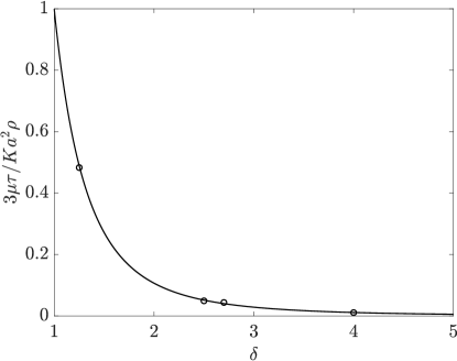
Figure 4: Optimal inertial response time as a function of special drifter buoyancy (circles) and least-squares fit of model (20).

With all Maxey–Riley parameters now set, we can proceed to analyze the trajectories of the special drifters. In Fig. 5 we depict special drifter (from left to right, mat, cuboid, sphere, and cube) trajectories along with trajectories (solid thin) resulting by integrating the full Maxey–Riley set (5) (solid bold), trajectories produced by the reduced Maxey–Riley set (12) (dot-dashed, nearly indistinguishable from bold solid), and trajectories resulting by integrating the latter with $\tau=0$ (dashed). The surface ocean velocity synthesis discussed in the preceding section is used to represent the water velocity ($v$) involved in each of the corresponding dynamical systems, while the air velocity ($v_{\mathrm{a}}$) is specified using the reanalyzed wind data involved in that synthesis. The initial velocities required to integrate the full Maxey–Riley set are taken to be equal to the velocities of the various drifters as obtained from differentiating their trajectories in time. Several observations are in order.

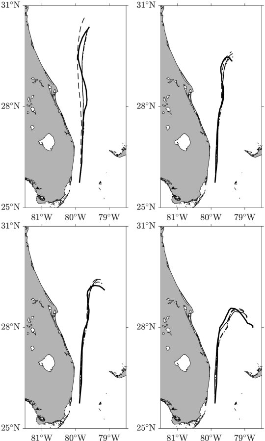
Figure 5: Special drifter (from left to right, mat, cuboid, sphere, and cube) trajectory (solid bold), and trajectories resulting by integrating the full Maxey–Riley set (solid thin), the reduced Maxey–Riley set (dot-dashed), and the latter with $\tau=0$ (dashed). The water velocity is taken as the surface ocean velocity synthesis in Fig. 2 and the air velocity as the reanalyzed wind involved in the synthesis. Initial velocities to integrate the full Maxey–Riley set are taken as the velocities of the special drifters. Parameters are given in Table 1.

First and foremost is the overall improved agreement between special drifter trajectories and Maxey–Riley trajectories relative to those resulting from integrating $v$ and the leeway model $v+\varepsilon v_{\mathrm{a}}$ with $\varepsilon=0.03$ (cf. Fig. 2). Indeed, the Maxey–Riley trajectories capture well both the drift of the mat, predominantly along the Florida Current, and the eastward turn unevenly experienced by the cuboid, sphere, and cube. The leeway model trajectories cannot represent the latter with, as we note below, a single leeway factor ($\varepsilon$) choice, and the trajectories of $v$ mainly represent the passive drift of ocean water along the Florida Current.

A second observation that follows from the inspection of Fig. 5 is that full Maxey–Riley trajectories coincide, virtually, with reduced Maxey–Riley trajectories. This indicates that convergence on the slow manifold is very fast. Consistent with this is the tendency of the Maxey–Riley trajectories to lie close, particularly the in the case of the sphere and the cube, to those produced by the reduced Maxey–Riley set with $\tau=0$. This by no means imply that the special drifters are not affected by inertia. Quite to the contrary, as we have clarified, $u$ depends on buoyancy and thus has inertial effects incorporated. This explains why a single choice of leeway factor $\varepsilon$ was not sufficient to explain the uneven effect of the ocean current and wind on the drift of the special drifters (recall Fig. 2).

An additional observation, which cannot be omitted, is that differences between observed and Maxey–Riley trajectories, albeit minor compared with those of the surface velocity synthesis and the leeway model, are visible in Fig. 5. There are several sources of uncertainty that contribute to produce differences between observed and Maxey–Riley trajectories. For instance, there are processes acting near the surface of the ocean that are not represented by the surface ocean flow synthesis considered here. The dominant component in this synthesis is the altimetry-derived velocity, which is too coarse to represent submesoscale motions and does not represent velocity shear between 15-m depth and the ocean surface. On the other hand, the Maxey–Riley set, as formulated, can only account for the potential contribution of wave-induced (Stokes) drift implicitly, by absorbing the corresponding wave-induced velocity in the water component of the carrying flow. The flow synthesis does not account for wave-induced motions as is constructed in such a way to minimize differences with velocities of drogued (GDP) drifters designed to keep wave-induced slip to very low levels (wind-plus-wave induced slip is less 1 $\mathrm{c}\mathrm{m}\,\mathrm{s}^{-1}$ in 10 $\mathrm{m}\,\mathrm{s}^{-1}$ wind Niiler, Davis, and White (1987)). In turn, coming from reanalysis, the near surface wind field cannot be expected to be fully represented. There is also uncertainty around the determination of the buoyancy of the special drifters, which can vary along a trajectory and this affect its determination even further.

Assessing the effects of the of uncertainty around the determination of the carrying flow field is not feasible. Yet we can, at least roughly, estimate those produced by that around the determination of the buoyancy of the special drifters. The result is presented in Fig. 6, which trajectories (in solid) overlaid on the area spanned by Maxey–Riley trajectories (shaded bands) resulting from allowing $\delta$ vary in an interval given by the value listed in Table 1 $\pm 10$% (the dashed curve, included for reference, has $\delta$ in the center of this interval). The width of this $\delta$-interval accounts very roughly for the error incurred in estimating the submerged depth of the special drifters in near-coastal water rather than at the deployment site in the Florida Current, and possibly too any changes in $\delta$ produced by water absorption or ambient water density variations along trajectories. Note that the special drifters and corresponding Maxey–Riley trajectories show consistency among over large portions to within $\delta$-induced uncertainty. In particular, most of the sphere’s trajectory falls quite well inside the $\delta$-induced uncertainty band around the corresponding Maxey–Riley trajectory. This encourages as to speculate that buoyancy uncertainty dominates the discrepancies between observed and simulated trajectories.

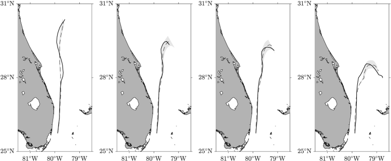
Figure 6: Special drifter (from left to right, mat, cuboid, sphere, and cube) trajectory (solid), Maxey–Riley trajectory with parameters as in Table 1 (dashed), and area spanned by Maxey–Riley trajectories resulting by allowing the buoyancy to range in an interval given by the value listed in Table 1 $\pm 10$% (shaded bands).

It is important to realize that differences between observed and simulated trajectories may never be completely eliminated. The fundamental reason for this stands on the unavoidable accumulation of errors and uncertainties, in addition to sensitive dependence on initial conditions, in any model, irrespective of how realistic Haller (2002). It is very remarkable then that despite this the Maxey–Riley set has performed so well when individual trajectories were compared.

VI Summary and concluding remarks

In this paper we have presented results of one of a series of experiments aimed at investigating the mechanism by which objects floating on the ocean surface are controlled by ocean currents and winds. The experiment consisted in deploying simultaneously in the same location drifting buoys of varied sizes, buoyancies, and shapes in the Florida Current, off the southeastern Florida Peninsula. The specially designed drifters described different trajectories, which were affected by a strong wind event within the first week of evolution since deployment. Consistent with the uneven response to the wind and ocean current action, the differences in the trajectories were explained as produced by the special drifters’ inertia. This was done by applying a recently proposed Maxey–Riley theory for inertial (i.e., buoyancy, finite-size) particle motion in the ocean Beron-Vera, Olascoaga, and Miron (2019a). Of buoyancy and finite size effects, the former were found to make the largest contribution to the inertial effects that controlled the special drifter motion.

The very good agreement between special drifter trajectories and those produced by the Maxey–Riley may be found surprising given the uncertainty around the determination of the carrying flow. Indeed, the ocean component of the flow was provided by a synthesis dominated by altimetry-derived velocity, while the atmospheric component was produced by winds from reanalysis. Both are admittedly limited. Furthermore, the Maxey–Riley set does not account for several potentially important aspects such as space and time dependence of the particle’s buoyancy or wave-induced drift.

We note that the Maxey–Riley set is found to be similarly successful in explaining the behavior of special drifters deployed in other sites of the North Atlantic as part of the experiments that complete the series. The drifters have similar characteristics as those deployed in the Florida Current. An important difference is that their trajectories lasted much longer than those discussed here, resulting in a much more stringent test of the validity of the Maxey–Riley set. A detailed analysis is underway and will be published elsewhere.

Finally, we took the opportunity of this paper to clarify the Maxey–Riley theory derived in Beron-Vera, Olascoaga, and Miron (2019a) with respect to the nature of the carrying flow and its domain of validity, and to propose a closure proposal for the determination of the parameters involved in terms of the carrying fluid system properties and particle characteristics was proposed. A corrigendum and addendum Beron-Vera, Olascoaga, and Miron (2019b) to Beron-Vera, Olascoaga, and Miron (2019a) is in progress. This will extend the theory to arbitrary large object’s buoyancies and seek to better justify the closure proposed here by means of direct numerical simulations.