Full-State Quantum Circuit Simulation
by Using Data Compression

Abstract.

Quantum circuit simulations are critical for evaluating quantum algorithms and machines. However, the number of state amplitudes required for full simulation increases exponentially with the number of qubits. In this study, we leverage data compression to reduce memory requirements, trading computation time and fidelity for memory space. Specifically, we develop a hybrid solution by combining the lossless compression and our tailored lossy compression method with adaptive error bounds at each timestep of the simulation. Our approach optimizes for compression speed and makes sure that errors due to lossy compression are uncorrelated, an important property for comparing simulation output with physical machines. Experiments show that our approach reduces the memory requirement of simulating the 61-qubit Grover’s search algorithm from 32 exabytes to 768 terabytes of memory on Argonne’s Theta supercomputer using 4,096 nodes. The results suggest that our techniques can increase the simulation size by 2$\sim$16 qubits for general quantum circuits.

1. Introduction

Classical simulation of quantum circuits is crucial for better understanding the operations and behaviors of quantum computation. Such simulations allow researchers and developers to evaluate the complexity of new quantum algorithms and validate quantum devices. The path toward building Noisy Intermediate-Scale Quantum (NISQ) (Preskill, 2018) machines such as IBM’s 50-qubit quantum computer and Google’s 72-qubit quantum computer (Kelly, 2018) will require intermediate-scale quantum circuit simulators to calibrate and verify the hardware.

Table 1. Examples of supercomputers, their total memory capacity, and the maximum number of qubits they can simulate for arbitrary circuits.

System	Memory (PB)	Max Qubits
Summit	2.8	47
Sierra	1.38	46
Sunway TaihuLight	1.31	46
Theta	0.8	45

Unfortunately, today’s practical full-simulation limit is 47 qubits (Table 1) (Strohmaier et al., 2018). The reason is that the number of quantum state amplitudes required for the full simulation increases exponentially with the number of qubits, making physical memory the limiting factor. Given $n$ quantum bits (qubits), we need $2^{n}$ amplitudes to describe the quantum system (Nielsen and Chuang, 2002). In order to describe the amplitudes precisely, double-precision complex numbers are used to represent the state of the quantum systems. As a result, the size of the quantum state in the simulation is $2^{n+4}$ bytes. Although 49-qubit simulations will become possible in the near future with the arrival of exascale supercomputers (Facility, 2019), a gap still remains between the size of classical simulation and the size of NISQ machines.

Several simulation techniques related to Feynman paths (Bernstein and Vazirani, 1997) and tensor network contractions (Boixo et al., 2017; Markov and Shi, 2008; Pednault et al., 2017) have been proposed to trade time for space complexity. Different approaches have different benefits and disadvantages. For Feynman paths method, both time and space complexity grow exponentially with the circuit depth, and thus this technique can simulate only shallow circuits. For tensor network simulation methods, since the time complexity grows exponentially with the underlying graph treewidth, these simulation techniques can only simulate the circuits with low treewidth. Some approaches calculate only a single amplitude or a partial state vector in order to be less restrictive on computational resources (Chen et al., 2018a; Chen et al., 2018b; Pednault et al., 2017; Boixo et al., 2017). As for quantum software development, several types of quantum applications require intermediate measurement (Bennett et al., 1996; Gottesman, 1997; Barends et al., 2014; Brassard, 1996). In addition, recent studies focus on quantum software debugging by inserting assertions in the middle of quantum programs (Huang and Martonosi, 2019). Tensor network simulation techniques do not effectively support intermediate measurement and full-state assertion checking for software debugging. At the same time, NISQ machines are evolving toward supporting deeper circuits with error mitigation techniques (Bonet-Monroig et al., 2018; Kandala et al., 2019; Endo et al., 2018; Sagastizabal et al., 2019), which may make full-state simulations of high-depth circuits more important. When trying to verify quantum hardware and software by using a full-state simulator, every qubit counts in maximum simulation size. Every qubit closer to physical machine sizes means 2X more state space that can be evaluated, or, conversely, 2X smaller gap in state space between the simulation and the physical hardware.

To simulate general circuits with higher qubit count and depth, we propose quantum circuit simulation techniques that can reduce the memory requirement of the full simulation by compressing quantum state amplitudes at runtime. Specifically, we apply data compression techniques to the quantum state vector during the simulation. Since we aim to simulate intermediate-scale general quantum circuits, we have to achieve a data compression ratio as high as possible, because the compression ratio is the key to increasing the number of qubits in the simulation. Our approach uses lossless compression, lossy compression, and adaptive error bounds to reduce the memory requirement of the simulation. In general, lossy compression algorithms lead to significantly higher compression ratios than do lossless compressors, while introducing errors to a certain extent. To minimize the error propagation and guarantee high-fidelity simulation results, we utilize both Zstandard lossless compressor (Collet, 2015) and an error-bounded tailored lossy compressor in our simulation framework.

Intuitively, one might be concerned that lossy compression would introduce correlated errors in our simulation output that would be very different from the kinds of errors that physical machines would experience. We will see, however, that our lossy compression is applied in an uncorrelated fashion. We shall also see that this has an added benefit of dramatically speeding up compression time.

Using our techniques, we are able to trade computation time and fidelity for memory space. We implement our techniques on Intel-QS, a full-state quantum circuit simulator developed by Intel (Smelyanskiy et al., 2016). Intel-QS is an MPI-based distributed high-performance quantum circuit simulator that can run on supercomputing systems. By orchestrating data compression techniques and full-state high-performance simulation techniques, our approach is capable of simulating intermediate-scale general quantum applications and hence obtain effective results of calibration, verification, and benchmarking for NISQ quantum machines.

Our approach integrates knowledge of quantum computation and data compression techniques to reduce the memory requirement of quantum circuit simulations such that our technique allows us to simulate a larger quantum system with the same memory capacity. We provide one more option in the set of tools to scale quantum circuit simulation. The main contributions of our work are as follows.

• We present a new technique to reduce memory requirements of full-state simulations of general quantum circuits by using data compression. Reducing memory requirements allows us to increase the number of qubits in our full-state simulations.

• We design a novel lossy compression method to optimize both compression ratios and compression speed for quantum circuit simulations. This lossy compression technique can be combined with several existing simulation techniques to further reduce the memory footprint.

• We implement our general quantum circuit simulation framework on the Theta supercomputer at Argonne National Laboratory (ANL).

• Our experimental results show that our approach reduces the memory requirement of simulating the 61-qubit Grover’s search quantum circuit from 32 exabytes to 768 terabytes of memory. Based on the state-of-the-art simulation techniques, the results suggest that our technique can increase the simulation size by 2 to 16 qubits for general quantum applications with 0.976 simulation fidelity on average.

Our paper is organized as follows. In Section 2, we introduce the basics of quantum computation and simulation as well as the data compression techniques. In Section 3, we present our simulation design. In Section 4, we describe our lossy compression technique, and in Section 5 we evaluate our approach. We discuss future directions and provide conclusions in Section 6.

2. Background and Related Work

In this section, we provide a brief overview of the quantum computation and discuss related work on quantum circuit simulations. We then present the relevant background on compression techniques.

2.1. Principles of Quantum Computation

A qubit is a two-level quantum system, and the state $\ket{\psi}$ can be expressed as

(1) $$\ket{\psi}=a_{0}\ket{0}+a_{1}\ket{1},$$

where $a_{0}$ and $a_{1}$ are complex amplitudes and $|a_{0}|^{2}+|a_{1}|^{2}=1$. $\ket{0}$, and $\ket{1}$ are two computational orthonormal basis states. The quantum state can also be represented as follows.

(2) $$\ket{\psi}=a_{0}\begin{bmatrix}1\\ 0\end{bmatrix}+a_{1}\begin{bmatrix}0\\ 1\end{bmatrix}=\begin{bmatrix}a_{0}\\ a_{1}\end{bmatrix}$$

More generally, the state of an $n$-qubit quantum system can be represented by using $2^{n}$ amplitudes, as follows.

(3) $$\ket{\psi}=a_{0...00}\ket{0...00}+a_{0...01}\ket{0...01}+...+a_{1...11}\ket{1...11}$$

The squared magnitudes have to sum up to 1, that is,

(4) $$\sum_{i}|a_{i}|^{2}=1.$$

In quantum computation, quantum gates are applied to the quantum system. All gates are represented in matrix form. General single-qubit gates and two-qubit controlled gates are known to be universal (DiVincenzo, 1995). Applying a single-qubit gate $U$ to the $k$th qubit can be represented by a unitary transformation

(5) $$A=I^{\otimes n-k-1}\otimes U\otimes I^{\otimes k},$$

where $I$ is a $2\times 2$ identity matrix and $U$ is a $2\times 2$ unitary matrix.

2.2. Quantum Circuit Simulation

Previous studies have provided various types of simulators (Quantiki, 2019). Generally, in order to simulate a quantum circuit with $n$ qubits and depth $d$, there are several simulation approaches (Aaronson and Chen, 2016; Bernstein and Vazirani, 1997; Markov and Shi, 2008). Different simulation approaches have different purposes and benefits.

Schrödinger algorithm. This strategy maintains the full-state vector in memory and updates the state vector in every time step (De Raedt et al., 2007; Smelyanskiy et al., 2016). Since the space grows exponentially with the number of qubits, the physical memory limits the simulation size. The time complexity is polynomial with the number of gates (or circuit depth), and hence this approach is capable of simulating arbitrary depth of circuits. This simulation approach can simulate the supremacy circuits of 45 qubits on the Cori II supercomputing system using 0.5 petabytes (Häner and Steiger, 2017), and Li et al. further optimize the simulator specifically for the 49-qubit supremacy circuits (Li et al., 2018).

Feynman paths algorithm. This approach calculates the amplitude $a_{x}$ for any $n$-bit string $x\in\{0,1\}^{n}$ by following all the paths from a final state to the initial state. For the Feynman paths algorithm, this approach requires $O(2^{dn})$ time to perform the simulation (Pednault et al., 2017), and hence this simulation technique is suitable only for low-depth quantum circuits.

Tensor network contractions. This approach uses tensor networks to represent quantum circuits (Markov and Shi, 2008; Biamonte and Bergholm, 2017; McCaskey et al., 2018). The time and space cost for contracting such tensor networks is exponential with the treewidth of the underlying graphs. Therefore, this approach is impractical to simulate large quantum circuits. Several studies have proposed to use tensor network simulation technique to simulate low-depth supremacy circuits (Boixo et al., 2017; Pednault et al., 2017; Chen et al., 2018a; Villalonga et al., 2020). To trade the simulation fidelity for computational resources, the approximate simulation is proposed (Markov et al., 2018; Boixo et al., 2017). The previous studies of approximate simulations target the overall circuit fidelity at 0.005 (Markov et al., 2018; Villalonga et al., 2020), but if we want to use the simulation results to help calibrate and validate the real machines, we might need higher circuit fidelity. As for quantum software development, several types of quantum applications require intermediate measurement (Bennett et al., 1996; Gottesman, 1997; Barends et al., 2014; Brassard, 1996). In addition, recent studies propose to insert assertions in quantum programs for software debugging by checking the full-state distribution (Huang and Martonosi, 2019). Tensor network simulation techniques do not effectively support intermediate measurement and full-state assertion checking.

Other strategies for simulating quantum circuits also exist. The Gottesman-Knill theorem (Gottesman, 1998) states that circuits consisting of only Clifford gates can be efficiently simulated in polynomial time, hence there are simulation techniques for the circuits with a restricted gate library (Goldberg and Guo, 2017; Gottesman, 1998; Aaronson and Gottesman, 2004; Bravyi and Gosset, 2016). In (Zulehner and Wille, 2018), the decision diagram is used to simulate circuits that consist of Clifford+T gates. This approach exploits redundancies in a quantum state to gain more compact representations. Approximate simulation techniques also have been proposed for circuits using only restricted gates (Zulehner et al., 2019; Zulehner and Wille, 2019; Bravyi and Gosset, 2016).

2.3. Data Compression Techniques

With the vast volumes of data being produced by extreme-scale scientific research and applications, various data compression techniques have been developed for years. Basically, scientific researchers mainly adopt two types of compressors: lossless compressors or error-bounded lossy compressors. Lossless compressors usually adopt both variable-length encoding algorithms (such as Huffman encoding (Huffman, 1952) and arithmetic encoding (Witten et al., 1987)) and dictionary coders such as LZ77/78 (Ziv and Lempel, 1977). In most cases, however, lossless compressors such as Gzip (Deutsch, 1996), Zstd (Collet, 2015), and Blosc (BlosC compressor, [n. d.]) cannot effectively compress scientific data because the ending mantissa bits of floating-point values are random such that it is hard to find exactly the same patterns in the data stream. Some studies (Di and Cappello, 2016a) show that lossless compressors always suffer from low compression ratios (around 2:1 in most cases), which is far less than enough for today’s extreme-scale high-performance computing (HPC) applications. Accordingly, error-bounded lossy compression has been widely treated as the best solution to such a big scientific data issue, because it not only can significantly reduce the data size but also can control the data distortion according to the user’s requirements.

Error-bounded lossy compressors may have distinct designs and implementations, so selecting the most appropriate compression technique is critical to our research. All existing error-bounded lossy compressors can be categorized into two models: data-prediction based and domain-transform based, which are described below.

• Data-prediction-based compression model. This model tries to predict each data point as accurately as possible based on its neighborhood in spatial or temporal dimension and then shrinks the data size by some coding algorithm such as data quantization (Tao et al., 2017) and bit-plane truncation. A typical example compressor is SZ (Liang et al., 2018), which involves four compression steps: (1) data prediction, (2) linear-scaling quantization, (3) entropy-encoding, and (4) lossless compression. The errors are introduced and controlled at step (2). Other examples include ISABELA (Lakshminarasimhan et al., 2013) and FPZIP (Lindstrom and Isenburg, 2006).

• Domain-transform-based compression model. This model needs to transform all the original data values to another nonorthogonal coefficient domain for decorrelation and then shrink the data size by applying some optimized coding algorithms such as embedded coding (Lindstrom, 2014). A typical example compressor is ZFP (Lindstrom, 2014), which performs the classic texture compression by leveraging three techniques in each $4^{d}$ block (where $d$ is the number of dimensions): (1) exponent alignment, (2) (non)orthogonal block transform, and (3) embedded coding. The compression errors (or distortion of data) are introduced and controlled only at step (3). The other two techniques are VAPOR (Clyne et al., 2007) and Sasaki et al.’s compressor (Sasaki et al., 2015), which both adopt the Wavelet transform in the domain transform step.

All the existing state-of-the-art error-bounded lossy compressors are designed or assessed mainly for visualization, so they are not optimized for the requirement of data fidelity and compression quality in the context of quantum computing simulation. In this sense, we first characterize the effectiveness of the existing state-of-the-art lossy compressors on quantum circuit simulation results and then exploit a fairly efficient compression method beyond the existing lossy compressors. In our study, we investigate two types of error controls, pointwise absolute error bound and pointwise relative error bound, because they have been supported by the existing state-of-the-art lossy compressors well.

• Absolute Error Bound (denoted by e). With this type of error control, the compression errors (defined as the difference between the original data value and its corresponding decompressed value) of all data points must be strictly limited in the required bound; in other words, $d^{\prime}_{i}$ must be in [$d_{i}-e,d_{i}+e$], where $d_{i}$ and $d_{i}^{\prime}$ refer to an original data value and the corresponding decompressed value, respectively.

• Relative Error Bound (denoted by $\epsilon$). With this type of error control, the data distortion must respect the following inequality for each data point: $|d_{i}-d_{i}^{\prime}|$$\leq$$\epsilon d_{i}$. Obviously, the smaller the original value is, the smaller the compression error it will get. The relative error bound is particularly useful to applications requiring multiple error controls depending on the data values.

3. Simulation Design

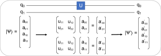
Figure 1. Example of two-qubit quantum state with single-qubit gate operations

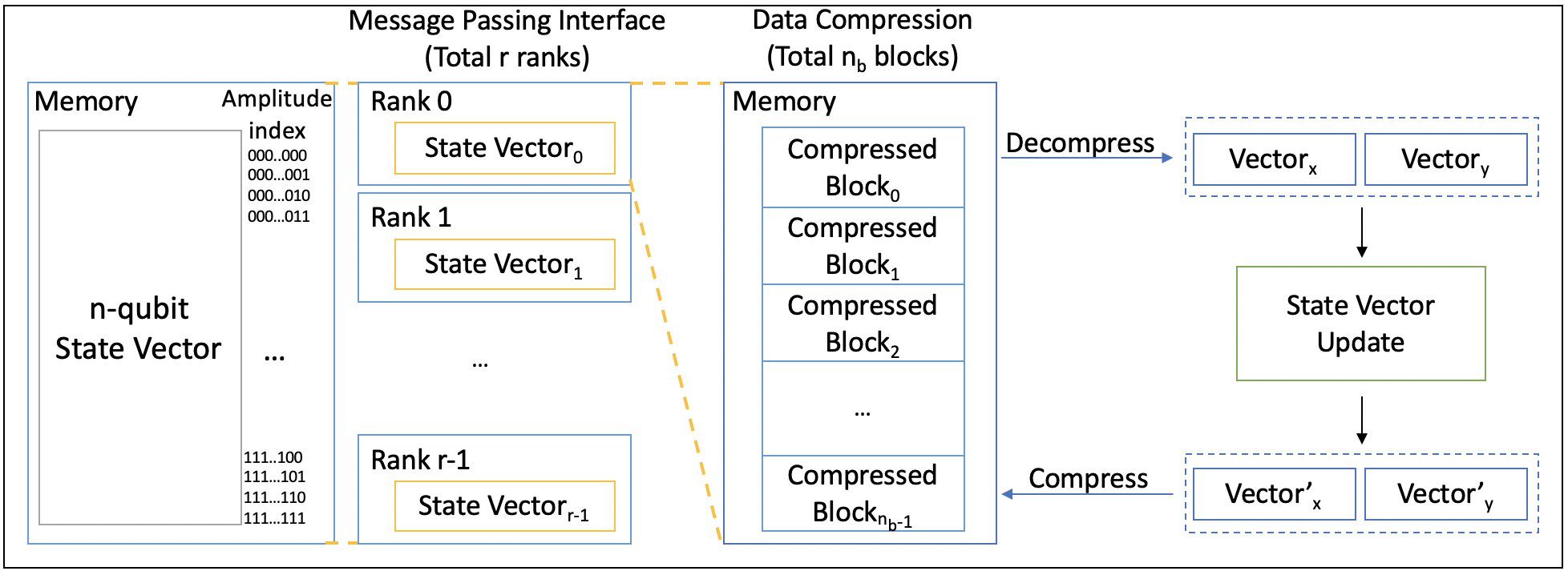
Figure 2. Simulation overview

We aim to simulate general quantum circuits with high fidelity. We integrate our compression techniques into the quantum circuit simulation such that the simulation scale can be increased with the same memory capacity. Our technique allows the Schrödinger-style simulation to trade the computation time and simulation accuracy for memory space by applying lossy compression techniques to state vectors. The lower compression error bound gives us the higher simulation fidelity, but the higher compression error bound will give us a higher compression ratio so that we can simulate the quantum circuits with larger numbers of qubits.

3.1. Overview of Our Simulation Flow

To demonstrate the practicality of our design, we integrate our compression techniques into Intel-QS (Smelyanskiy et al., 2016), a distributed quantum circuit simulator on a classical computer.

As mentioned in Section 2, applying a single-qubit gate to the $k$th qubit can be represented by a unitary transformation $A=I^{\otimes n-k-1}\otimes U\otimes I^{\otimes k}$. In the simulation, however, we do not need to build the entire unitary matrix $A$ to perform the gate operation. Figure 1 shows an example of applying a single-qubit gate to a two-qubit system. Applying a gate $U$ to the first qubit corresponds to applying the $2\times 2$ unitary matrix to every pair of amplitudes, whose subscript indices have 0 and 1 in the first bit and all remaining bits are the same. In the same way, performing a single-qubit gate to the second qubit is to apply the unitary to every pair of amplitudes whose subscript indices differ in the second bit. More extensively, applying a single-qubit gate to the $k\text{-th}$ qubit of an $n$-qubit quantum system is to apply the unitary to every pair of amplitudes whose subscript indices have 0 and 1 in the $k\text{-th}$ bit, while all other bits remain the same.

(6) $$\begin{bmatrix}a^{\prime}_{*...*0_{k}*...*}\\ a^{\prime}_{*...*1_{k}*...*}\end{bmatrix}=\begin{bmatrix}u_{11}&u_{12}\\ u_{21}&u_{22}\end{bmatrix}\begin{bmatrix}a_{*...*0_{k}*...*}\\ a_{*...*1_{k}*...*}\end{bmatrix}$$

As for a generalized two-qubit controlled gate, the unitary is applied to a target qubit $t$ if the control qubit $c$ is set to $\ket{1}$; otherwise $t\text{th}$ is unmodified.

(7) $$\begin{bmatrix}a^{\prime}_{*1_{c}...*0_{t}*...*}\\ a^{\prime}_{*1_{c}...*1_{t}*...*}\end{bmatrix}=\begin{bmatrix}u_{11}&u_{12}\\ u_{21}&u_{22}\end{bmatrix}\begin{bmatrix}a_{*1_{c}...*0_{t}*...*}\\ a_{*1_{c}...*1_{t}*...*}\end{bmatrix}$$

Figure 2 shows an overview of our simulation design. The Message Passing Interface (MPI) (Gropp et al., 1999) is used to execute the simulation in parallel.

Assuming we simulate $n$-qubit systems and have $r$ ranks in total, the state vector is divided equally on $r$ ranks. To reduce the memory requirement, we further divide the partial state vector into $n_{b}$ blocks on each rank. Each block is stored in compressed format on the memory. To complete a gate operation, we need to apply matrix multiplication to the pair of amplitudes whose subindices are 0 and 1 at the target qubit position, so at most two blocks are decompressed, $Vector_{x}$ and $Vector_{y}$, and then update the state vectors. After all the amplitudes in $Vector_{x}$ and $Vector_{y}$ are updated, we compress the state vectors and move to the next two blocks. Once all the blocks have been updated, a gate operation is completed.

In this way, the total number of bytes required for the simulation of a rank is as follows:

(8) $$nbBytes=\sum_{i}sizeof(CB_{i})+2(\frac{2^{n+4}}{r\times n_{b}}),$$

where $CB_{i}$ is the $i$th compressed block.

3.2. MCDRAM Memory Configuration

Multichannel DRAM (MCDRAM) is a high-bandwidth, low-capacity memory, packaged with the Intel Xeon Phi processor (Sodani, 2015). Because several repeated compression and decompression operations are involved in the simulation, we can achieve the performance improvement by utilizing MCDRAM. Every time the block is decompressed, we decompress the state vectors to MCDRAM. To allocate memory in MCDRAM, we use mkl_malloc function to acquire memory space. This memory allocation strategy directly improves the performance of compression, gate operation, and decompression. To achieve this, we set the machine to equal mode, 50% cache and 50% flat.

3.3. Integration Details

We build our compressor as a C library and add it into the Intel-QS building process. In the initialization of the simulation process, we create the state vectors in blocks, and compress them as compressed blocks. During the simulation, if the process needs to update the state vector, it calls our compressor library to decompress the block to the pre-allocated MCDRAM. After the state vector update, the block is compressed, and the process moves to the next block.

Since we allow decompression of only two blocks for each rank at the same time, we must select the corresponding blocks to be decompressed. For $n$-qubit systems, assuming we have $r$ ranks and each block contains $b$ amplitudes, the amplitude index string can be divided into three segments (Figure 3). When we execute a single-qubit gate computation on the target qubit position $q$, we find the corresponding blocks according to the segment $q$ belongs to.

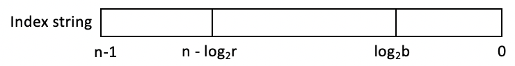
Figure 3. Amplitude index segments

• $q<log_{2}b:$ Both amplitudes are in the same block.

• $n-log_{2}r\leq q\leq log_{2}b:$ Both amplitudes are in the same rank but with different blocks. We can use the number $q$ to find the corresponding blocks in the rank.

• $q>n-log_{2}r:$ The pair of amplitudes are in the different ranks. The blocks have to be exchanged between different ranks.

Two-qubit gate operations are similar to single-qubit gate operations, but we modify the amplitudes only when the control qubit is set to $\ket{1}$. According to the position of the control qubit $c$, we also have three cases to determine whether the amplitudes should be modified:

• $c<log_{2}b:$ If $c$th bit is 0, the amplitude is left unmodified.

• $n-log_{2}r\leq c\leq log_{2}b:$ If $c$th bit is 0, the whole block is left unmodified.

• $c>n-log_{2}r:$ If $c$th bit is 0, the whole rank is left unmodified.

3.4. Compressed Block Cache

For most of the quantum circuits, the amplitudes may share the same value (Zulehner and Wille, 2018). By exploiting redundancies in the quantum state, we can reduce the computation time significantly by constructing a compressed block cache.

Figure 4. Compressed block cache line

Figure 4 shows the contents of a compressed block cache line. The first element $(OP)$ is the gate operation and the target qubit position. The second and third elements $(CB_{1},CB_{2})$ are the compressed blocks before the gate operation. The rest of the elements $(CB^{\prime}_{1},CB^{\prime}_{2})$ are the compressed blocks after the gate operation. Each rank maintains a memory space for the compressed block cache with 64 cache lines. When a gate operation is executed, our computation procedure first checks whether the pattern $(OP,CB_{1},CB_{2})$ is in the cache. If there is a cache hit, then the computation is done by directly returning the blocks $(CB^{\prime}_{1},CB^{\prime}_{2})$, and thus the performance is improved by reducing the compression, computation, and decompression time.

The cache replacement policy is least recently used. If there is no redundancy in the quantum state, the cache hit rate will be 0, and this will introduce the cache miss penalty in our simulation. Thus, our simulator will disable the compressed block cache if the cache hit rate is always zero.

3.5. Simulation Checkpoint

In general, most supercomputing systems have a 24-hour wall-time limit. This runtime constraint puts a circuit depth limit on the simulation. However, one can save the compressed blocks before terminating the job and then resume the task by loading the compressed blocks in the next job submission.

3.6. MPI Configuration

To understand the performance under different MPI rank configuration, we run the 35-qubit random circuit simulation with various ranks per node (Figure 5). On the KNL nodes, each node has 64 cores and 256 threads. We found that the setting of 128 ranks per node gives the best performance.

Figure 5. Normalized execution time for running 35-qubit random circuit simulations.

3.7. Variable Error Bound Compression

To keep the simulation accuracy, we use the lossless compression Zstd(Collet, 2015) in the beginning of the simulation when the compression ratio is still high enough to fit all compressed blocks in the memory space. During the simulation, the quantum state becomes more and more complicated, and hence the lossless compression ratio is lower. When the compression ratio is too low to fit all compressed blocks in the memory, our simulation will use lossy compression to compress the state vectors. To control the error, we use a pointwise relative error bound to compress the state vector. This compression mode guarantees that the decompressed data point $|D^{\prime}|$ must be in the range of $(|D(1-\delta)|,|D|)$, where $D$ is the original data and $\delta$ is the error bound. In this work, we have five different levels of error bounds: 1E-5, 1E-4, 1E-3, 1E-2, and 1E-1. Whenever the compression ratio is not enough, the error bound is relaxed to the next level (larger error). We give a detailed discussion about our lossy compression technique in the next section.

3.8. Lower Bounds on Simulation Accuracy

Since lossy compression is used in our simulations, information is lost with every lossy compression, causing a decrease in the simulation’s overall accuracy. The accuracy of our simulation can be quantified by the state fidelity, a measure of the similarity of two quantum states (Nielsen and Chuang, 2002).

The fidelity takes values between $0$ and $1$, with higher fidelity indicating greater similarity between the two states. A fidelity of $1$ would indicate that the two quantum states are the same. The pure state fidelity between the ideal output state, $\psi_{ideal}$, and the output state from our simulation, $\psi_{sim}$, can be described by the following simplified equation (Nielsen and Chuang, 2002).

(9) $$F(ideal,sim)=|\langle\psi_{ideal}|\psi_{sim}\rangle|$$

Since the errors are bounded in our simulation, the fidelity can be estimated by propagating the maximum error bounds at each gate to calculate the maximum decrease in fidelity (from the ideal fidelity of 1) that comes from each lossy compression and then finding their combined impact on the overall maximum decrease in fidelity. Suppose that a gate has a percentage error of $\delta$. Then if a complex amplitude $a_{i}$ in the ideal state vector is represented as $a+bi$, the corresponding amplitude after our lossy compression in the simulation can be represented by $a^{\prime}+b^{\prime}i$, where $|a^{\prime}|\geq|a(1-\delta)|$ and $|b^{\prime}|\geq|b(1-\delta)|$. Thus, we see that the state fidelity can be calculated as follows:

(10) $$F(ideal,sim)=|\langle\psi_{ideal}|\psi_{sim}\rangle|\geq\sum_{i=0}^{2^{n}-1}a_{i}^{2}(1-\delta)=1-\delta.\vspace{-2mm}$$

So we see that the minimum fidelity drops by a factor of $(1-\delta)$ after applying a lossy compression with a maximum percentage error bound of $\delta$. Suppose that for the $i$th gate, the error bound is $\delta_{i}$ on the lossy compression. Then the lower bound on the fidelity after applying this compression will drop to $(1-\delta_{i})$ times the lower bound on the fidelity calculated before lossy compression on this gate. Combining the contributions of all the gates in the simulation allows us to calculate the lower bound on the simulation fidelity as

(11) $$F(ideal,sim)\geq\prod_{i}{(1-\delta_{i})}.$$

If all the $\delta_{i}$ were 0, the simulation fidelity would be 1, which makes sense because our simulation would then be identical to the simulation without lossy compression against which we are calculating the fidelity. As mentioned before, in our simulation with lossy compression, the error bounds $\delta_{i}$ can be set to 0 (lossless), 1E-5, 1E-4, 1E-3, 1E-2, and 1E-1. Figure 6 shows how fidelities change with the number of gates when different error levels are applied.

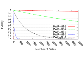
Figure 6. Minimum bounds for fidelity with an increasing number of gates at different error levels

4. Adaptive Compression Optimized for Quantum Circuit Simulation

In this section, we propose a novel error-bounded compression method that can significantly control memory footprint for full-state quantum circuit simulations that were unreachable before.

4.1. Assessment of Existing Error-Bounded Lossy Compressors

First, we explore the best solution from among the existing compressors for the quantum circuit simulations. We choose SZ (Di and Cappello, 2016b; Zou et al., 2019), FPZIP (Lindstrom and Isenburg, 2006), and ZFP (Lindstrom, 2014) in our exploration because they have been confirmed as the best error-bounded compressors on many scientific datasets (Di and Cappello, 2016b; Zou et al., 2019; Lu et al., 2018).

We perform the assessment using two well-known quantum circuits: a quantum approximate optimization algorithm (QAOA) (Farhi et al., 2014) and the random circuit proposed by Google to show quantum supremacy (Boixo et al., 2018). In this analysis, we run 36 qubits for both circuits and denote them as qaoa_36 and sup_36, respectively.

As discussed in Section 2.3, there are two types of error bounds, both of which have been widely used by scientific applications, so we evaluate the compression ratios for quantum circuit simulation data based on both types of errors. Since each rank involves hundreds or thousands of data blocks each having different value ranges, we perform the compression based on the absolute error bound in the regard of value range in our evaluation, without loss of generality. That is, we set the absolute error bound to a fixed percentage of the value range in each block. For instance, 1E-2 means 1% of the value range in the following figures.

Figure 7 presents the compression ratios of SZ and ZFP based on different absolute error bounds. FPZIP is missing in this figure because it does not support an absolute error bound. We can see that SZ always leads to one or two orders of magnitude higher compression ratios than ZFP does at every error bound. For instance, on qaoa_36, SZ can lead the compression ratios up to about 100:1, while ZFP’s compression ratios are always less than 10:1. For the dataset sup_36, the compression ratios of SZ and ZFP are about 28$\sim$126 and 4.25$\sim$12.6, respectively.

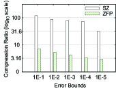
(a) qaoa_36

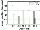
(b) sup_36

Figure 7. Compression ratio of SZ vs. ZFP (absolute error)

For the pointwise relative error bound, for ZFP, we transform the original data to the logarithm domain and then compress the transformed data with absolute error bounds, for fairness of the comparison. Such a log-preprocessing-based compression has been validated as the best way to do the pointwise relative-error-bounded compression (Xin Liang, 2018). As for FPZIP, it provides a so-called precision number (=4$\sim$64) to control the pointwise relative error bound. The larger the precision number is, the lower the pointwise relative error bound obtained. We set the precisions to 16, 18, 22, 24, and 28 for FPZIP in our experiments because they correspond to the pointwise relative error bounds of 1E-1, 1E-2, 1E-3, 1E-4, and 1E-5 approximately. Figure 8 clearly shows that SZ always leads to much higher compression ratios than do the other two compressors with the same pointwise relative error bounds.

(a) qaoa_36

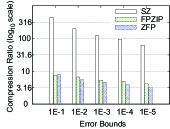
(b) sup_36

Figure 8. Compression ratio of SZ,FPZIP,ZFP (relative error)

Based on our analysis, we conclude that SZ is superior to the other two compressors. The key reason is as follows. For ZFP, it substantially replies on the high smoothness of data, especially when the error bounds are set to a relatively low value. However, the quantum simulation data are not smooth at all, as illustrated in Figure 9, such that the domain-transform in ZFP would totally lose its effectiveness, leading to poor compression ratios. The key difference between FPZIP and SZ is that the former adopts a totally different encoding method, unlike SZ adopting linear-scaling quantization + Huffman encoding + Zstd. In what follows, we treat SZ as the baseline and propose a new lossy compression method that is more effective on the quantum circuit simulation data.

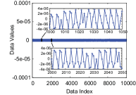
(a) qaoa_36

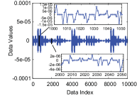
(b) sup_36

Figure 9. Illustration of Value changes of quantum circuit simulation data: the data exhibit a high spikiness such that existing lossy compressors cannot work effectively.

4.2. Optimizing the Compression Strategy

In our work, we adopt a hybrid, adaptive compression pipeline to control the memory footprint while keeping the high fidelity of the simulation results and relatively low time overhead. Specifically, we observe that at the early stage of the simulation, a large majority of the data are zero. In this situation, the lossless compressor Zstd can also get a satisfactory compression ratio, without any loss of data fidelity. Although SZ leads to much higher compression ratios in this situation, it may introduce data distortion, causing degraded fidelity unexpectedly. As the simulation goes on, however, the simulation data will become more and more complicated, such that Zstd will suffer from low compression ratios. In this situation, the error-bounded lossy compressor is helpful in controlling the memory footprint while keeping a high fidelity of simulation results. Thus, we adopt both Zstd and error-bounded lossy compression during each entire simulation. More details are in Section 3.7.

Developing a fast, effective error-bounded lossy compressor is critical to the overall simulation results (including fidelity and simulation time). In particular, we need to use a pointwise relative error bound to do the compression, as discussed in Section 3. To this end, we explored a battery of novel compression strategies to optimize both the compression ratios and compression speed for quantum circuit simulations, as described below.

Solution A (SZ 2.1): This solution is the state-of-the-art error-bounded lossy compressor - SZ (Di and Cappello, 2016b; Tao et al., 2017; Zou et al., 2019). In the context of quantum circuit simulations, the data can be treated only as a 1D array. In SZ 2.0, the pointwise relative-error-bounded compression involves the following steps: (1) logarithm data transform; (2) absolute-error-bounded compression on log-transformed data (Lorenzo prediction (Ibarria et al., 2003) + quantization (Tao et al., 2017)); (3) Huffman encoding; and (4) Zstd lossless compression. Since log-transform is expensive, the SZ development team developed SZ 2.1 leveraging a table lookup method to accelerate the compression significantly (Zou et al., 2019), without degrading the compression ratios. However, the compression/decompression speed still cannot meet the expected level for quantum circuit simulations (to be shown later), which motivates us to further explore a new, faster compression method instead.

Solution B (SZ 2.1 with complex type supported): Quantum state amplitudes are stored in the form of complex data type, in which the real numbers and imaginary numbers are stored alternatively, such that the prediction accuracy would be degraded to a certain extent, leading to limited compression ratios. Accordingly, Solution B improves the prediction accuracy by performing the prediction on the real numbers and imaginary numbers, respectively. In addition, we set the maximum number of quantization bins to 16,384 (unlike the default setting of 65,536 in SZ 2.1), which can significantly improve the compression/decompression rate (to be shown later).

Solution C (XOR leading-zero data reduction + bit-plane truncation + Zstd): Solution B can improve the compression ratios in some cases, but its compression speed is still lower than expected such that the total simulation would slow significantly compared with the original compression-free execution. To reduce the compression/decompression time significantly, we developed Solution C, a simple yet efficient compression pipeline that is particularly suitable for quantum circuit simulation. This method involves three key steps. For each data point, it first leverages XOR leading-zero data reduction method (Burtscher and Ratanaworabhan, 2009; Di and Cappello, 2016b), which uses a two-bit code to record the number of exactly the same bytes between the current value and its preceding value. Then the algorithm truncates the insignificant bit-planes based on the required relative error bound $\epsilon$. Specifically, the significant number of bits can be calculated as follows.

(12) $$Sig\_Bit\_Count=Bit\_Count(Sign\&Exp)-EXP(\epsilon),$$

where $EXP(\epsilon)$ refers to the exponent of the relative error bound $\epsilon$ (e.g., $EXP(0.01)$=$-7$) and $Bit\_count(Sign\&Exp)$ is the total number of bits used to represent sign and exponent in the IEEE 754 format (e.g., it is equal to 12 for double precision). We then adopt Zstd lossless compression to shrink the data significantly.

Solution D (Reshuffle + Solution C): Since the simulation data are stored in the complex data type (i.e., real number and imaginary number alternatively), one plausible idea is to reorganize the data into real numbers and imaginary numbers separately before compressing the data. Such a reshuffle step may help improve compression ratio especially when the real numbers and imaginary numbers are located in different non-overlapped value ranges. The reason is that in Solution C, the last step Zstd involves a dictionary-matching stage (LZ77 (Ziv and Lempel, 1977)) leveraging potential repeated patterns in the data streams and the reshuffling step that separates the real numbers and imaginary numbers may improve the pattern matching to a certain extent. Accordingly, we developed Solution D, which might have higher compression ratios with a slightly lower compression/decompression rate.

We evaluate all the four solutions by doing the compression and decompression with the two simulation datasets qaoa_36 and sup_36. Figure 10 presents the compression ratios of the four solutions. We can see that the classic compressor SZ 2.1, either supporting complex type (Solution B) or not (Solution A), suffers from about 30%$\sim$50% lower compression ratios than do Solutions C and D. The likely reason is that the simulation data exhibit spiky changes (as illustrated in Figure 9) such that the SZ compressor always suffers from low prediction accuracy. Besides, we note that the solution C may lead to slightly higher compression ratios than does the solution D in some cases, which also makes sense as explained as follows. Note that the only difference between these two solutions is the extra reshuffle step in the solution D. This step might affect the compression ratio only because of the LZ77 stage in the last step Zstd of the two solutions, as analyzed previously. With this in mind, the compression ratio actually may not change significantly in between since the pattern matching efficiency for the two solutions could be very similar. On the one hand, Zstd improved LZ77 by adopting a pretty large window size. On the other, the real numbers and imaginary numbers are of the similar value ranges (as shown in Figure 9), such that the reshuffling step may not induce more regular data. In this sense, the solution C and D can be deemed having comparative compression ratios on the QC simulation datasets.

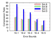
(a) qaoa_36

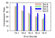
(b) sup_36

Figure 10. Compression ratio of 4 solutions (relative error)

We present the compression and decompression rate in Figure 11 (single-core performance). This figure clearly shows that Solutions B, C, and D have much higher compression rates and decompression rates than the classic SZ 2.1 (Solution A) does. The key reason Solution B is faster than Solution A is that it predicts the data in terms of the complex data type, which may get higher prediction accuracy, thus leading to faster encoding thereafter. Moreover, we set a lower maximum number of quantization bins in Solution B such that it keeps a relatively high compression rate in the case with low relative error bounds such as 1E-5. The reason the Solutions C and D run much faster than Solutions A and B do is that they totally remove the three costly steps—prediction, quantization, and Huffman encoding—in the compression. We can also observe that Solution C is slightly faster than Solution D because of the extra reshuffle step in Solution D.

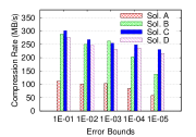
(a) qaoa_36 (Cmpr)

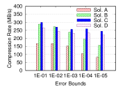
(b) sup_36 (Cmpr)

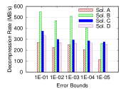
(c) qaoa_36 (Decmpr)

(d) sup_36 (Decmpr)

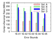
(e) qaoa_36 (Cmpr+Decmpr)

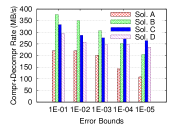
(f) sup_36 (Cmpr+Decmpr)

Figure 11. Compress/decompression rates (relative error)

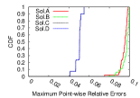
(a) qaoa_36:PWR=1E-1

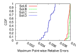
(b) qaoa_36:PWR=1E-2

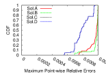
(c) qaoa_36:PWR=1E-3

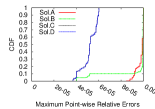
(d) qaoa_36:PWR=1E-4

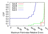
(e) qaoa_36:PWR=1E-5

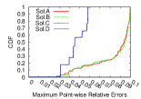
(f) sup_36:PWR=1E-1

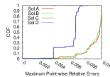
(g) sup_36:PWR=1E-2

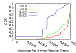
(h) sup_36:PWR=1E-3

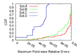
(i) sup_36:PWR=1E-4

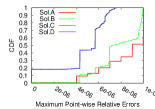
(j) sup_36:PWR=1E-5

Figure 12. Distribution of maximum relative errors on compression of qaoa_36 and sup_36 (Solution C and D overlap)

We present in Figure 12 the distribution of the maximum compression error (pointwise relative errors) per data block for all four compression solutions on qaoa_36 and sup_36, respectively. Similar to the previous evaluations, the experimental dataset comes from one rank involving hundreds of data blocks (each with 1,048,576 complex-type data points, bringing a total of 16 MB per block).

From Figure 12 we observe that all four solutions respect the compression errors well in terms of different pointwise relative error bounds (1E-1$\sim$1E-5). We note that the error distribution curves of Solutions C and D overlap, which is explained as follows. In fact, they both avoid the data prediction and quantization step such that the compression errors have nothing to do with the order of the data points. The only difference between them is the extra reshuffle step in Solution D. Thus they have exactly the same compression errors in each block.

Moreover, we note that Solutions C and D exhibit much lower compression errors than do Solutions A and B in general. The reason is as follows. As illustrated in Figure 13 (a), Solutions A and B both adopt the data prediction and linear-scaling quantization (Tao et al., 2017). Specifically, they predict each data point and then approximate its value by the error-bound-quantized distance (Tao et al., 2017) between the true raw value and the predicted value. Note that the compression errors are determined by the difference between the decompressed values and the true values (as shown in Figure 13 (a)). Hence, if the error bound is relatively small, the quantization bin size would be small too, then the true values would be located at a rather random postion in a quantization bin because of the likely large distance between the predicted value and true value, thus leading to a uniform distribution. By comparison, Solutions C and D calculate the significant bit-planes based on user-required pointwise relative errors, and each bit-plane spans a certain value range. As illustrated in Figure 13 (b) (with a single-precision value 3.9921875 as an example), truncating different bit planes will lead to discrete decompressed values and relative errors. Suppose the relative error bound is set to 0.01, then we need to keep 15 leading bits and the decompressed value would be 3.96875 with a relative error of 0.005871, which is actually lower than the error bound 0.01. That is, the compression errors of the solutions C and D are generally somewhat lower than the desired error bound.

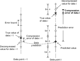
(a) Prediction and quantization in solution A/B

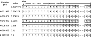
(b) Discrete relative errors when truncating bits in solution C/D

Figure 13. Illustrating why Solution C/D leads to lower compression errors than Solution A/B

Such overpreservation of error can be observed more clearly by plotting the distribution of normalized compression errors compared with the error bounds for Solution C, as presented in Figure 14. We plot the cumulative distribution function (CDF) of the normalized pointwise relative errors compared with the corresponding error bounds for one random block of data, because too many data points are involved in the whole simulation and other blocks actually exhibit similar error distributions. In the figure we can observe that (1) all compression errors are indeed confined within the required relative error bound; (2) the compression errors follow a uniform distribution; and (3) most of the compression errors are actually much lower than the required error bound, bringing an extra benefit to the control of data distortion in the simulation.

(a) qaoa_36

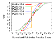
(b) sup_36

Figure 14. Distribution of normalized compression errors (Solution C)

Moreover, the solution C leads to non-correlated compression errors (point-wise relative errors) for the quantum circuit simulation datasets. The reason is that the relative errors are determined by the high-order bit-values in the truncated insignificant bit-planes. Since the quantum circuit simulation data exhibit a rather high randomness (as presented in Figure 9), the truncation errors are supposed to be fairly random as well. We confirm this point by calculating the lag-1 autocorrelation coefficients of the compression errors. The autocorrelation value is always in [-1,1]; the closer to zero, the higher level of non-autocorrelation is. Our evaluation shows that the autocorrelation value often ranges in [-1E-4,1E-4] if a large majority of original raw data are non-zeros in the dataset, testifying the high non-correlation feature of the solution C.

Based on this analysis, we can conclude that Solution C is a fairly good tradeoff, which can obtain a high compression ratio, low compression time and decompression time, and low compression errors with non-correlation feature. Accordingly, Solution C is our final error-bounded lossy compressor to be used in our experiments.

5. Evaluation

5.1. Experimental Setup

For multinode evaluation, we performed our simulation on the Theta supercomputer at Argonne National Laboratory. Theta consists of 4,392 nodes, each node containing a 64-core Intel®Xeon Phi^TM processor 7230 with 16 gigabytes of high-bandwidth in-package memory (MCDRAM) and 192 GB of DDR4 RAM (Parker et al., 2017). The bandwidth of the MCDRAM is 400GB/s, and the average latency is 154 ns (Asai, 2016). On Theta, there are wall-time limits for each jobs with different numbers of nodes. The wall-time limits are 3, 6, and 24 hours for jobs of 128 nodes, 256 nodes, and 1,024 nodes, respectively. For jobs running exceeding wall-time limits, we use our checkpoint design, described in Section 3.5, to complete the simulation.

For single-node experiments, we run our simulation on a single 64-core Intel®Xeon Phi^TM processor 7210 (KNL) in the Joint Laboratory for System Evaluation (JLSE) at Argonne. There is no wall-time limit on the system.

In this evaluation, we set 128 ranks per node. As described in Section 3, the state vector on each rank is divided into multiple blocks, each containing 1,048,576 amplitudes, which means each block is 16 MB. Since each rank decompresses at most 2 blocks on MCDRAM at the same time, we need to allocate $128\times 2\times 16MB=4GB$ of memory on MCDRAM. Thus, we configure the memory mode by using --attrs mcdram=equal to operate 50% MCDRAM as flat memory and the other 50% as cache (Jeffers and Reinders, 2013).

5.2. Scalability

We evaluate the scaling behavior by using a basic program that applies a Hadamard gate on each qubit. Figure 15 shows the normalized execution time for running different sizes of simulations on a single node. The scaling of our simulation technique for 51-qubit quantum circuit running on different numbers of nodes is depicted in Figure 16. For simulations of real applications that requires more time in compression, decompression, and computation, the scaling is expected to be better.

Figure 15. Normalized execution time for running various sizes of simulations on a single node.

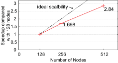
Figure 16. Scaling behavior of applying Hadamard gates on a 51-qubit system on Theta.

5.3. Benchmarks

To show the results against real applications, we choose multiple important quantum applications as our benchmarks. The benchmarks are selected to have different program characteristics in order to show that our simulation could work with arbitrary quantum circuits. Our approach performs well for both shallow-circuit and deep-circuit applications. The initial state is $\ket{0}^{\otimes n}$. The programs we use for our benchmarking include the following.

• Grover: Grover’s search algorithm is for database search, and it leads to significant speedups compared with classical search algorithms (Grover, 1996; JavadiAbhari et al., 2015). Our benchmark uses Grover’s search algorithm to find the square root number (JavadiAbhari et al., 2015), and thus the oracle consists of X and Toffoli gates.

• Random circuit sampling: The circuit is proposed by Google to show the quantum supremacy, and we follow the rules to construct the random circuits (Boixo et al., 2018). Since our approach is not optimized for the circuits, we do not plan to run the random circuits with many layers. Thus, the circuit depth is 11 in our experiments.

• QAOA: The quantum approximate optimization algorithm is a hybrid quantum-classical variational algorithm. Our benchmark uses QAOA to solve MAXCUT on a random 4 regular graph problem (Farhi et al., 2014). QAOA is an important circuit because it is one of the most promising quantum algorithms in the NISQ era (Preskill, 2018).

• QFT: This is the quantum circuit for quantum Fourier transform (JavadiAbhari et al., 2015), which is an important function in many quantum algorithms (Shor’s algorithm (Shor, 1999), phase estimation algorithm (Cleve et al., 1998), and the algorithm for hidden subgroup problem (Jozsa, 2001)), and this is a deep circuit. We randomly apply X gate to the initial state as the input for the QFT in our experiments.

Table 2. Experimental results. The first row shows the memory requirements of the simulations without our techniques. The ratios of our system memory sizes to the required memory sizes are presented in the fourth row. The fifth row provides the simulation time and the breakdown. The minimum compression ratio during the simulation is shown in the last row.

Benchmark	Grover			Random Circuit Sampling				QAOA			QFT
Number of Qubits	61	59	47	$5\times 9$	$6\times 7$	$6\times 6$	$7\times 5$	45	43	42	36
(Memory Requirement)	(32 EB)	(8 EB)	(2 PB)	(512 TB)	(64 TB)	(1 TB)	(512 GB)	(512TB)	(128 TB)	(64 TB)	(1 TB)
Number of Gates	314	310	305	227	261	165	208	394	344	336	3258
Number of Nodes	4096	4096	128	1024	128	1	1	1024	256	128	1
Total System Memory	768 TB	768 TB	24 TB	192 TB	24 TB	192 GB	192 GB	192TB	48 TB	24 TB	192 GB
(Sys Mem / Req.)	(0.002%)	(0.009%)	(1.17%)	(37.5%)	(37.5%)	(18.75%)	(37.5%)	(37.5%)	(37.5%)	(37.5%)	(18.75%)
Total Time (Hour)	8.14	3.48	0.49	4.87	8.64	7.96	6.23	13.34	5.83	8.65	78.98
Compression Time	1.87%	4.59%	2.04%	55.79%	40.26%	59.10%	58.57%	50.66%	44.97%	41.02%	57.86%
Decompression Time	1.87%	3.73%	4.08%	31.47%	22.19%	33.78%	30.59%	26.46%	27.64%	25.52%	37.68%
Communication Time	32.7%	20.98%	36.73%	0.12%	0.57%	0.02%	0.03%	3.03%	0.22%	0.23%	2.56%
Computation Time	63.47%	70.70%	57.15%	12.60%	36.97%	7.08%	10.8%	19.84%	27.16%	33.22%	1.9%
Time per Gate (Sec)	93.34	40.49	5.78	64.69	119.22	173.65	107.86	121.91	61.02	92.64	87.27
Simulation Fidelity	0.996	0.996	1	0.987	0.993	0.933	0.985	0.895	0.999	0.999	0.962
Compression Ratio	$7.39\times 10^{4}$	$8.26\times 10^{4}$	$1.06\times 10^{4}$	6.03	9.40	8.16	10.05	5.38	4.85	9.25	21.34

5.4. Experimental Results

We present our main results in Table 2. We run benchmarks with the total system memory capacities much less than the theoretical memory requirements to manifest the strength of our approach.

Our first benchmark application is Grover’s search algorithm with 47, 59 and 61 qubits. Previously, 61-qubit simulations of general quantum applications were thought to be impossible because of infeasible memory requirements. Using our methods, the state vectors can be compressed with high compression ratios because the amplitude values of the state vectors of this application are similar and regular, and hence our approach can use only 768 TB to successfully perform the simulation of 61-qubit Grover’s search algorithm, which theoretically requires 32 EB to execute the full-state simulation. We also use our technique to complete the 47-qubit Grover’s search algorithm simulation using 24 TB instead of 2 PB, the memory requirement without our technique. Next, we present the simulation of Google’s quantum supremacy random circuits. Since our method exploits non-uniformity and structure in quantum computations, it does not work as well on random circuits. If we run many layers of the circuits, we have to drop the simulation fidelity to meet the available memory capacity. Thus, we present the simulation results of depth of 11 random circuits. Although our simulation technique is not designed specifically for the supremacy circuits, our approach can simulate the circuit with 42 qubits by using 48 TB, and simulate the circuit with 45 qubits by using 192 TB. The next benchmark is QAOA. Since QAOA is an important quantum application, it is critical to the simulation of QAOA circuits with limited memory capacity. In fact, we can get higher compression ratios and still get successful results because QAOA is robust to low-fidelity. Finally, the results with QFT circuits show that our techniques are effective for simulating high-depth circuits and compress the state vectors with more than 21X compression ratios, with a fidelity of 0.962.

For the quantum applications we choose, we show that our technique can simulate the circuits with high fidelity. Among the selected benchmarks, random circuits use more entanglement than others. Since our techniques compress the state vector, more entanglement leads to less compressible vectors. Thus, our technique does better when there is less entanglement.

5.5. Discussion

We successfully increase the maximum simulation size from 45 qubits to 61 qubits for the Grover’s search circuit simulation on the Argonne Theta supercomputer using less than 0.8 PB. As for simulations of the other quantum applications, we have compression ratios from 4.85X to 21.34X. The results provide evidence that we are able to simulate those applications with 47 to 49 qubits on Theta. In other words, for simulations of general circuits, our approach can increase the simulation size by 2 to 16 qubits. In this work, we seek to achieve high-fidelity simulation results for general circuits. For different purposes that do not require high-simulation fidelity, the compression ratios and simulation size would be further increased.

We use the compression ratios to estimate our approach on the Summit supercomputer (Wells et al., 2016) at Oak Ridge National Laboratory (ORNL). The expected maximum simulation size for general circuits is 63 qubits. In 2021, we will have the exascale supercomputing system Aurora (Facility, 2019) at Argonne. The estimated maximum simulation size will be increased from 48 qubits to 64 qubits. Our compression techniques can combine with other simulation techniques (Chen et al., 2018b; Häner and Steiger, 2017; Li et al., 2018; Zulehner et al., 2019; Zulehner and Wille, 2019) to scale quantum circuit simulation.

We trade time and slight fidelity for memory space. This trade-off makes the classical simulation of several quantum circuits possible, while the simulation time grows linearly with the number of gates. The time complexity is polynomial with circuit depth.

6. Conclusion and Future Work

Our approach performs full-state simulation of general quantum circuits using data compression techniques. This method allows the Schrödinger-style simulation to trade time and simulation fidelity for memory space to increase the simulation size. Our compression techniques can combine with other simulation techniques (Chen et al., 2018b; Häner and Steiger, 2017; Li et al., 2018; Zulehner et al., 2019; Zulehner and Wille, 2019). By using our lossy compression, we can compress state vectors and reduce memory footprints significantly compared with the existing techniques (Smelyanskiy et al., 2016; Häner and Steiger, 2017). The compression errors are not correlated to the data, and hence the errors might be used to further simulate noise on real devices. The modern noise simulations add errors to perfect simulations. However, we could further adapt our lossy compression errors to noise models and then build a simulation which models noise naturally. In addition, we plan to implement our simulator on GPU-based supercomputing systems to reduce the compression and decompression time.

In summary, we have described our simulation techniques to reduce the memory requirement of full-state quantum circuit simulations by using data compression techniques. Our method provides a new option in the set of simulation tools to scale quantum circuit simulations. We propose a novel lossy compression technique to optimize compression ratios and compression speed for quantum circuit simulations. Using our approach, the memory requirement of simulating the 61-qubit Grover’s search algorithm is reduced from 32 exabytes to 768 terabytes of memory on the Argonne Theta supercomputer using 4,096 nodes. We also present experimental results of random circuits, QAOA, and QFT simulations to show that our technique can achieve general circuit simulations. The compression ratio results further suggest that our technique can increase the simulation size by 2 to 16 qubits for general quantum applications. Our simulator provides a platform for quantum software debugging and quantum hardware validation.

References

- (1)
- Aaronson and Chen (2016) Scott Aaronson and Lijie Chen. 2016. Complexity-theoretic foundations of quantum supremacy experiments. arXiv preprint arXiv:1612.05903 (2016).
- Aaronson and Gottesman (2004) Scott Aaronson and Daniel Gottesman. 2004. Improved simulation of stabilizer circuits. Physical Review A 70, 5 (2004), 052328.
- Asai (2016) Ryo Asai. 2016. MCDRAM as High-Bandwidth Memory (HBM) in Knights Landing processors: developers guide. Colfax International (2016).
- Barends et al. (2014) Rami Barends, Julian Kelly, Anthony Megrant, Andrzej Veitia, Daniel Sank, Evan Jeffrey, Ted C White, Josh Mutus, Austin G Fowler, Brooks Campbell, et al. 2014. Superconducting quantum circuits at the surface code threshold for fault tolerance. Nature 508, 7497 (2014), 500.
- Bennett et al. (1996) Charles H. Bennett, David P. DiVincenzo, John A. Smolin, and William K. Wootters. 1996. Mixed-state entanglement and quantum error correction. Phys. Rev. A 54 (Nov 1996), 3824–3851. Issue 5. https://doi.org/10.1103/PhysRevA.54.3824
- Bernstein and Vazirani (1997) Ethan Bernstein and Umesh Vazirani. 1997. Quantum complexity theory. SIAM Journal on computing 26, 5 (1997), 1411–1473.
- Biamonte and Bergholm (2017) Jacob Biamonte and Ville Bergholm. 2017. Tensor networks in a nutshell. arXiv preprint arXiv:1708.00006 (2017).
- BlosC compressor ([n. d.]) BlosC compressor. [n. d.]. http://blosc.org/. Online.
- Boixo et al. (2018) Sergio Boixo, Sergei V Isakov, Vadim N Smelyanskiy, Ryan Babbush, Nan Ding, Zhang Jiang, Michael J Bremner, John M Martinis, and Hartmut Neven. 2018. Characterizing quantum supremacy in near-term devices. Nature Physics 14, 6 (2018), 595.
- Boixo et al. (2017) Sergio Boixo, Sergei V Isakov, Vadim N Smelyanskiy, and Hartmut Neven. 2017. Simulation of low-depth quantum circuits as complex undirected graphical models. arXiv preprint arXiv:1712.05384 (2017).
- Bonet-Monroig et al. (2018) X Bonet-Monroig, R Sagastizabal, M Singh, and TE O’Brien. 2018. Low-cost error mitigation by symmetry verification. Physical Review A 98, 6 (2018), 062339.
- Brassard (1996) Gilles Brassard. 1996. Teleportation as a quantum computation. arXiv preprint quant-ph/9605035 (1996).
- Bravyi and Gosset (2016) Sergey Bravyi and David Gosset. 2016. Improved classical simulation of quantum circuits dominated by Clifford gates. Physical review letters 116, 25 (2016), 250501.
- Burtscher and Ratanaworabhan (2009) M. Burtscher and P. Ratanaworabhan. 2009. FPC: A High-Speed Compressor for Double-Precision Floating-Point Data. IEEE Trans. Comput. 58, 1 (Jan 2009), 18–31. https://doi.org/10.1109/TC.2008.131
- Chen et al. (2018a) Jianxin Chen, Fang Zhang, Mingcheng Chen, Cupjin Huang, Michael Newman, and Yaoyun Shi. 2018a. Classical simulation of intermediate-size quantum circuits. arXiv preprint arXiv:1805.01450 (2018).
- Chen et al. (2018b) Zhao-Yun Chen, Qi Zhou, Cheng Xue, Xia Yang, Guang-Can Guo, and Guo-Ping Guo. 2018b. 64-qubit quantum circuit simulation. Science Bulletin (2018).
- Cleve et al. (1998) Richard Cleve, Artur Ekert, Chiara Macchiavello, and Michele Mosca. 1998. Quantum algorithms revisited. Proceedings of the Royal Society of London. Series A: Mathematical, Physical and Engineering Sciences 454, 1969 (1998), 339–354.
- Clyne et al. (2007) John Clyne, Pablo Mininni, Alan Norton, and Mark Rast. 2007. Interactive desktop analysis of high resolution simulations: application to turbulent plume dynamics and current sheet formation. New Journal of Physics 9, 301 (2007), 1–29.
- Collet (2015) Yann Collet. 2015. Zstandard - Real-time data compression algorithm. http://facebook.github.io/zstd/ (2015).
- De Raedt et al. (2007) Koen De Raedt, Kristel Michielsen, Hans De Raedt, Binh Trieu, Guido Arnold, Marcus Richter, Th Lippert, H Watanabe, and N Ito. 2007. Massively parallel quantum computer simulator. Computer Physics Communications 176, 2 (2007), 121–136.
- Deutsch (1996) L Peter Deutsch. 1996. GZIP file format specification version 4.3.
- Di and Cappello (2016a) Sheng Di and Franck Cappello. 2016a. Fast error-bounded lossy HPC data compression with SZ. In 2016 IEEE International Parallel and Distributed Processing Symposium (IPDPS). IEEE, 730–739.
- Di and Cappello (2016b) Sheng Di and Franck Cappello. 2016b. Fast Error-Bounded Lossy HPC Data Compression with SZ. In IPDPS 2016. 730–739.
- DiVincenzo (1995) David P DiVincenzo. 1995. Two-bit gates are universal for quantum computation. Physical Review A 51, 2 (1995), 1015.
- Endo et al. (2018) Suguru Endo, Simon C Benjamin, and Ying Li. 2018. Practical quantum error mitigation for near-future applications. Physical Review X 8, 3 (2018), 031027.
- Facility (2019) Argonne Leadership Computing Facility. 2019. Aurora Supercomputer. https://www.alcf.anl.gov/programs/aurora-esp. Online. Accessed: 2019-04-06.
- Farhi et al. (2014) Edward Farhi, Jeffrey Goldstone, and Sam Gutmann. 2014. A quantum approximate optimization algorithm. arXiv preprint arXiv:1411.4028 (2014).
- Goldberg and Guo (2017) Leslie Ann Goldberg and Heng Guo. 2017. The complexity of approximating complex-valued Ising and Tutte partition functions. computational complexity 26, 4 (2017), 765–833.
- Gottesman (1997) Daniel Gottesman. 1997. Stabilizer codes and quantum error correction. arXiv preprint quant-ph/9705052 (1997).
- Gottesman (1998) Daniel Gottesman. 1998. The Heisenberg representation of quantum computers. arXiv preprint quant-ph/9807006 (1998).
- Gropp et al. (1999) William D Gropp, William Gropp, Ewing Lusk, and Anthony Skjellum. 1999. Using MPI: portable parallel programming with the message-passing interface. Vol. 1. MIT press.
- Grover (1996) Lov K Grover. 1996. A fast quantum mechanical algorithm for database search. arXiv preprint quant-ph/9605043 (1996).
- Häner and Steiger (2017) Thomas Häner and Damian S Steiger. 2017. 0.5 petabyte simulation of a 45-qubit quantum circuit. In Proceedings of the International Conference for High Performance Computing, Networking, Storage and Analysis. ACM, 33.
- Huang and Martonosi (2019) Yipeng Huang and Margaret Martonosi. 2019. Statistical assertions for validating patterns and finding bugs in quantum programs”. In 2019 ACM/IEEE 46th Annual International Symposium on Computer Architecture (ISCA). IEEE.
- Huffman (1952) D. A. Huffman. 1952. A Method for the Construction of Minimum-Redundancy Codes. Proceedings of the IRE 40, 9 (Sep. 1952), 1098–1101. https://doi.org/10.1109/JRPROC.1952.273898
- Ibarria et al. (2003) Lawrence Ibarria, Peter Lindstrom, Jarek Rossignac, and Andrzej Szymczak. 2003. Out-of-core compression and decompression of large n-dimensional scalar fields. Computer Graphics Forum 22, 3 (2003), 343–348.
- JavadiAbhari et al. (2015) Ali JavadiAbhari, Shruti Patil, Daniel Kudrow, Jeff Heckey, Alexey Lvov, Frederic T Chong, and Margaret Martonosi. 2015. ScaffCC: Scalable compilation and analysis of quantum programs. Parallel Comput. 45 (2015), 2–17.
- Jeffers and Reinders (2013) James Jeffers and James Reinders. 2013. Intel Xeon Phi coprocessor high performance programming. Newnes.
- Jozsa (2001) Richard Jozsa. 2001. Quantum factoring, discrete logarithms, and the hidden subgroup problem. Computing in science & engineering 3, 2 (2001), 34.
- Kandala et al. (2019) Abhinav Kandala, Kristan Temme, Antonio D Córcoles, Antonio Mezzacapo, Jerry M Chow, and Jay M Gambetta. 2019. Error mitigation extends the computational reach of a noisy quantum processor. Nature 567, 7749 (2019), 491.
- Kelly (2018) Julian Kelly. 2018. A preview of Bristlecone, Google’s new quantum processor. Google Research Blog 5 (2018).
- Lakshminarasimhan et al. (2013) Sriram Lakshminarasimhan, Neil Shah, Stephane Ethier, Seung-Hoe Ku, Choong-Seock Chang, Scott Klasky, Rob Latham, Rob Ross, and Nagiza F Samatova. 2013. Isabela for effective in situ compression of scientific data. Concurrency and Computation: Practice and Experience 25, 4 (2013), 524–540.
- Li et al. (2018) Riling Li, Bujiao Wu, Mingsheng Ying, Xiaoming Sun, and Guangwen Yang. 2018. Quantum supremacy circuit simulation on Sunway taihuLight. arXiv preprint arXiv:1804.04797 (2018).
- Liang et al. (2018) X. Liang, S. Di, D. Tao, S. Li, S. Li, H. Guo, Z. Chen, and F. Cappello. 2018. Error-Controlled Lossy Compression Optimized for High Compression Ratios of Scientific Datasets. In 2018 IEEE International Conference on Big Data (Big Data). 438–447. https://doi.org/10.1109/BigData.2018.8622520
- Lindstrom (2014) Peter Lindstrom. 2014. Fixed-rate compressed floating-point arrays. IEEE Transactions on Visualization and Computer Graphics 20, 12 (2014), 2674–2683.
- Lindstrom and Isenburg (2006) Peter Lindstrom and Martin Isenburg. 2006. Fast and efficient compression of floating-point data. IEEE Transactions on Visualization and Computer Graphics 12, 5 (2006), 1245–1250.
- Lu et al. (2018) T. Lu, Q. Liu, X. He, H. Luo, E. Suchyta, J. Choi, N. Podhorszki, S. Klasky, M. Wolf, T. Liu, and Z. Qiao. 2018. Understanding and Modeling Lossy Compression Schemes on HPC Scientific Data. In 2018 IEEE International Parallel and Distributed Processing Symposium (IPDPS). 348–357. https://doi.org/10.1109/IPDPS.2018.00044
- Markov et al. (2018) Igor L Markov, Aneeqa Fatima, Sergei V Isakov, and Sergio Boixo. 2018. Quantum supremacy is both closer and farther than it appears. arXiv preprint arXiv:1807.10749 (2018).
- Markov and Shi (2008) Igor L Markov and Yaoyun Shi. 2008. Simulating quantum computation by contracting tensor networks. SIAM J. Comput. 38, 3 (2008), 963–981.
- McCaskey et al. (2018) Alexander McCaskey, Eugene Dumitrescu, Mengsu Chen, Dmitry Lyakh, and Travis Humble. 2018. Validating quantum-classical programming models with tensor network simulations. PloS one 13, 12 (2018), e0206704.
- Nielsen and Chuang (2002) Michael A Nielsen and Isaac Chuang. 2002. Quantum computation and quantum information.
- Parker et al. (2017) Scott Parker, Vitali Morozov, Sudheer Chunduri, Kevin Harms, Chris Knight, and Kalyan Kumaran. 2017. Early Evaluation of the Cray XC40 Xeon Phi system ‘Theta’ at Argonne. Technical Report. Argonne National Lab.(ANL), Argonne, IL (United States).
- Pednault et al. (2017) Edwin Pednault, John A Gunnels, Giacomo Nannicini, Lior Horesh, Thomas Magerlein, Edgar Solomonik, and Robert Wisnieff. 2017. Breaking the 49-qubit barrier in the simulation of quantum circuits. arXiv preprint arXiv:1710.05867 (2017).
- Preskill (2018) John Preskill. 2018. Quantum Computing in the NISQ era and beyond. Quantum 2 (2018), 79.
- Quantiki (2019) Quantiki. 2019. A list of QC simulators. https://quantiki.org/wiki/list-qc-simulators. Online.
- Sagastizabal et al. (2019) Ramiro Sagastizabal, Xavier Bonet-Monroig, Malay Singh, MA Rol, CC Bultink, X Fu, CH Price, VP Ostroukh, N Muthusubramanian, A Bruno, et al. 2019. Error mitigation by symmetry verification on a variational quantum eigensolver. arXiv preprint arXiv:1902.11258 (2019).
- Sasaki et al. (2015) Naoto Sasaki, Kento Sato, Toshio Endo, and Satoshi Matsuoka. 2015. Exploration of Lossy Compression for Application-Level Checkpoint/Restart. In IPDPS 2015. 914–922.
- Shor (1999) Peter W Shor. 1999. Polynomial-time algorithms for prime factorization and discrete logarithms on a quantum computer. SIAM review 41, 2 (1999), 303–332.
- Smelyanskiy et al. (2016) Mikhail Smelyanskiy, Nicolas PD Sawaya, and Alán Aspuru-Guzik. 2016. qHiPSTER: the quantum high performance software testing environment. arXiv preprint arXiv:1601.07195 (2016).
- Sodani (2015) Avinash Sodani. 2015. Knights Landing (KNL): 2nd generation Intel® Xeon Phi processor. In 2015 IEEE Hot Chips 27 Symposium (HCS). IEEE, 1–24.
- Strohmaier et al. (2018) Erich Strohmaier, Jack Dongarra, Horst Simon, Martin Meuer, and Hans Meuer. 2018. TOP500 list. https://www.top500.org/lists/2018/11/. (2018).
- Tao et al. (2017) Dingwen Tao, Sheng Di, Zizhong Chen, and Franck Cappello. 2017. Significantly improving lossy compression for scientific data sets based on multidimensional prediction and error-controlled quantization. In Parallel and Distributed Processing Symposium (IPDPS), 2017 IEEE International. IEEE, 1129–1139.
- Villalonga et al. (2020) Benjamin Villalonga, Dmitry Lyakh, Sergio Boixo, Hartmut Neven, Travis S Humble, Rupak Biswas, Eleanor Rieffel, Alan Ho, and Salvatore Mandrà. 2020. Establishing the quantum supremacy frontier with a 281 pflop/s simulation. Quantum Science and Technology (2020).
- Wells et al. (2016) Jack Wells, Buddy Bland, Jeff Nichols, Jim Hack, Fernanda Foertter, Gaute Hagen, Thomas Maier, Moetasim Ashfaq, Bronson Messer, and Suzanne Parete-Koon. 2016. Announcing Supercomputer Summit. (6 2016).
- Witten et al. (1987) Ian H. Witten, Radford M. Neal, and John G. Cleary. 1987. Arithmetic Coding for Data Compression. Commun. ACM 30, 6 (June 1987), 520–540. https://doi.org/10.1145/214762.214771
- Xin Liang (2018) Dingwen Tao Zizhong Chen Franck Cappello Xin Liang, Sheng Di. 2018. Efficient Transformation Scheme for Lossy Data Compression with Point-wise Relative Error Bound. In CLUSTER. IEEE.
- Ziv and Lempel (1977) J. Ziv and A. Lempel. 1977. A universal algorithm for sequential data compression. IEEE Transactions on Information Theory 23, 3 (May 1977), 337–343. https://doi.org/10.1109/TIT.1977.1055714
- Zou et al. (2019) XiangYu Zou, Tao Lu, Wen Xia, Xuan Wang, Weizhe Zhang, Sheng Di, Dingwen Tao, and Franck Cappello. 2019. Accelerating Relative-error Bounded Lossy Compression for HPC datasets with Precomputation-Based Mechanisms. In Proceedings of the 35th International Conference on Massive Storage Systems and Technology (MSST19). IEEE.
- Zulehner et al. (2019) Alwin Zulehner, Philipp Niemann, Rolf Drechsler, and Robert Wille. 2019. Accuracy and Compactness in Decision Diagrams for Quantum Computation. In Design, Automation and Test in Europe.
- Zulehner and Wille (2018) Alwin Zulehner and Robert Wille. 2018. Advanced simulation of quantum computations. IEEE Transactions on Computer-Aided Design of Integrated Circuits and Systems (2018).
- Zulehner and Wille (2019) Alwin Zulehner and Robert Wille. 2019. Matrix-Vector vs. Matrix-Matrix Multiplication: Potential in DD-based Simulation of Quantum Computations. Quantum 1, 1 (2019), 1–1.