Non-Redundant OFDM Receiver Windowing for 5G Frames & Beyond

Abstract

Contemporary receiver (RW-OFDM) algorithms have limited adjacent channel interference (ACI) rejection capability under high delay spread and small fast Fourier transformation (FFT) sizes. cyclic prefix (CP) is designed to be longer than the maximum excess delay (MED) of the channel to accommodate such algorithms in current standards. The robustness of these algorithms can only be improved against these conditions by adopting additional extensions in a new backward incompatible standard. Such extensions would deteriorate the performance of high mobility vehicular communication systems in particular. In this paper, we present a low-complexity Hann RW-OFDM scheme that provides resistance against ACI without requiring any intersymbol interference (ISI)-free redundancies. While this scheme is backward compatible with current and legacy standards and requires no changes to the conventionally transmitted signals, it also paves the way towards future spectrotemporally localized and efficient schemes suitable for higher mobility vehicular communications. A Hann window effectively rejects unstructured ACI at the expense of structured and limited inter-carrier interference (ICI) across data carriers. A simple maximum ratio combining (MRC)- successive interference cancellation (SIC) receiver is therefore proposed to resolve this induced ICI and receive symbols transmitted by standard transmitters currently in use. The computational complexity of the proposed scheme is comparable to that of contemporary RW-OFDM algorithms, while ACI rejection and bit-error rate (BER) performance is superior in both long and short delay spreads. Channel estimation using Hann RW-OFDM symbols is also discussed.

I Introduction

Next generation cellular communication standards beyond 5G mobile communication are planned to schedule non-orthogonal sub-frames, referred to as numerologies, in adjacent bands[1]. Numerologies, in their current definition, refer to - (CP-OFDM) waveforms using different subcarrier spacings, and in some cases, various CP rates[2]. Different numerologies interfere with one-another[3] and ACI becomes the factor limiting data rates if the interfering block outpowers the desired block at the intended receiver[4].

Nodes can reject ACI by filtering[5] or windowing[6] the received signal. Filtering requires matched filtering operation at the both ends of the communication system for optimal performance[7]. If not already implemented at both nodes, this requires modifying the device lacking this function, which is unfeasible for user equipments that are produced and in-use. The additional complex multiplication and addition operations required to filter the signal increase the design complexity of the modem, which in turn increase the chip area, production cost, power consumption, and operational chip temperature and reduces the lifetime of the device and battery[8]. Introducing these operations at the next generation NodeB (gNB) can be justified to improve system performance, however the takeaways may cause Internet of Things (IoT) devices to fall short of their key performance indicators and is undesirable [9].

Receiver windowing is another method proposed to reduce ACI absorption[6] and is extensively studied in the literature[10]. Conventional RW-OFDM algorithms require an abundant periodic extension of the transmitted signal that is free from multipath echoes of the previous symbol to maintain orthogonality of the system[11]. However, such an extension may not always be available or may be little, especially in vehicular communication channels requiring shorter symbol durations[12]. Trying to utilize these algorithms in these conditions would require adding an additional extension, as shown in Fig. 1b. However, modifying the symbol structure defined in both 4G and 5G mobile communication standards [2], shown in Fig. 1a, with such an extension breaks orthogonality with all other devices that use the standard frame structure[1]. Even if any gain for the desired user itself can be made possible by incorporating such extension for receiver windowing, introducing such elevated interference to others is not allowed by the current standards[13]. Furthermore, both ends of the communication must be aware of and agree to make such a change.

(a)

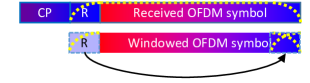
(b)

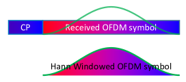
(c)

Figure 1: (a) Standard symbol structure, (b) Symbol structure needed to utilize conventional receiver windowing algorithms effectively in channels with long delay spread, and (c) Hann receiver windowing using standard symbol structures.

Another potential problem regarding additional extensions for windowing is the increase in the effective symbol duration which reduces the effective symbol rate. Due to the time variation of the channel in high mobility systems, the additional extensions not only cause a direct reduction in data rate but also either further cuts the data rate back when relative pilot overhead is increased to mitigate the reduction in absolute pilot periodicity or reduces capacity due to the channel estimation errors when no modification is done[14]. In order to achieve reliable high mobility vehicular communications, there is an apparent need to shorten the cyclic extensions instead of further elongating them.

A receiver windowing approach that utilizes the CP disturbed by multipath interference to reject ACI while conserving the legacy frame structure was proposed in [15]. Reducing ACI with this approach comes at the cost of introducing ISI, which consists of the sum of the low powered contributions from all subcarriers of the previous symbol. The computational complexity of canceling the ISI is high due to the large number of interfering components. Furthermore, this approach is not effective with shorter CP durations that are associated with vehicular communication numerologies. Consider Fig. 2, which shows the power spectral densitys of the the sixth subcarrier from the band-edge of different orthogonal frequency division multiplexing (OFDM) variations and window functions. The PSD labeled as "Slepian[16] Win." in Fig. 2a is obtained by performing receiver windowing operation presented in [11] on an extended CP numerology[2] using the entire CP duration of a small subcarrier spacing, long duration OFDM symbol. In this case, the window works as expected and is able to confine the spectrum within the resource block (RB) as intended, and consistently fades throughout the spectrum. However, if the same algorithm is applied to a short duration vehicular numerology with normal CP overhead, as shown in Fig. 2b, the window underperforms and provides a limited benefit over the standard rectangular window even if the whole CP duration is still used. Furthermore, the PSD behaves inconsistently throughout the spectrum due to the limited resolution especially for the subcarriers of the edgemost RB as presented, oscillating to high powers away from the subcarrier of interest. Also note that this is the performance upper bound for a normal CP overhead. If a shorter window duration is used to utilize part of the CP for its actual purpose to mitigate multipath channel and limit ISI, the performance reduces further. filtered- (F-OFDM) [5] does not suffer from the same problem, but requires changes at the transmitting device and is computationally complex. $N$-Continuous (NC-OFDM) [17] can be utilized by all devices in the band to consistently reduce the ACI levels regardless of symbol duration, but this scheme also requires changes at both transmitting and receiving devices, and also introduces in-band interference as seen in Fig. 2. There is an apparent need for a reception algorithm that does not modify the standard transmitter, has low computational complexity, and is robust against delay spread without requiring extensions, and is not affected by the FFT size.

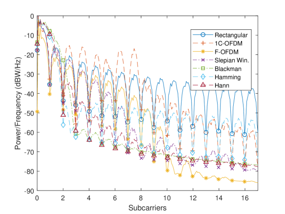
(a)

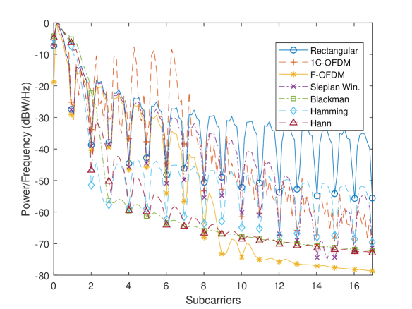
(b)

Figure 2: The PSDs of OFDM schemes and window functions applied to a (a) long duration OFDM symbol with extended CP and (b) short duration OFDM symbol with normal CP rates. The markers indicate FFT sampling points.

In a regular OFDM based system, if no redundancy is used for windowing, and a receiver window function other than rectangular is used, the zero crossings of the window’s frequency response differs from that of the transmitted subcarriers[10]. This causes heavy ICI between the received subcarriers, resulting in problems greater than the avoided ACI [6]. Attempting to cancel the resulting ICI yields little return if the ICI consists of weak contributions from numerous subcarriers, and the computational complexity and success of the cancellation renders such implementation impractical in general. Some window functions commonly used in signal processing reveal special cases[18] if the windowing operation depicted in Fig. 1c is performed, limiting the number of interfering subcarriers which may be exploited to possibly enable gains. A strong candidate is the Blackman window function, which provides promising ACI rejection seen in Fig. 2. However, the main lobe of the Blackman window function spans 2 adjacent subcarriers on the shown right hand side spectrum and 2 more on the not-visible left hand side, thereby including high-power ICI from a total of 4 subcarriers. This results in computationally intensive reception and limits capacity gains. Another strong candidate is the Hamming window function, which only interferes with the closest 2 adjacent subcarriers, hence enabling lower-complexity reception. The ACI rejection performance of Hamming window function in the subcarriers that immediately follow the main lobe is also unmatched. However, considering the ACI rejection performance throughout the rest of the spectrum and the power of the inflicted ICI due to windowing, the Hann window function is distinguished from other candidates and is chosen in this study to satisfy this apparent need. A similar investigation during the design of the Global System for Mobile Communications (GSM) system led in favor of the gaussian minimum shift keying (GMSK) pulse shapes that are inherently non-orthogonal only with a finite number of symbols around them and signal-to-interference ratio (SIR) degradation is manageable in severe multiple access multipath channel conditions, instead of other candidates that are ideally orthogonal but suffer severe SIR degradation once this orthogonality is lost due to multiple access multipath channel [19]. Because of the aforementioned spectral features, Hann windowing similarly converts a complex ACI problem, with its out-of-band rejection performance comparable to optimum windowing as shown in Fig. 2a, to a manageable ICI problem requiring little computational complexity at the receiver[20, 21].

We present a novel transceiver algorithm that mitigates the ICI resulting from Hann windowing. This algorithm performs well regardless of OFDM symbol duration, CP duration or delay spread. The algorithm is solely a receiver algorithm that can be used to receive the signals transmitted from a conventional legacy transmitter using any modulation. Therefore the systems using either of the proposed algorithms are interoperable with future and legacy standards. This algorithm consists of maximizing signal to interference plus noise ratio (SINR) first using MRC, afterwards mitigating the ICI using a soft decision turbo SIC equalizer. Furthermore, the computational complexity of the algorithm is less than or comparable to [11], while a higher performance is achieved in most conditions. A block diagram of the proposed method is presented in Fig. 3.

Figure 3: The block diagram of the proposed scheme, highlighting the modifications to the standard receiver structure with dashed blocks (standard transmitter is not modified).

Our contributions in this work are as follows:

• A redundancy free RW-OFDM scheme that outperforms prior art without requiring changes to the standard frame structure regardless of channel conditions is proposed. The proposed scheme has high ACI rejection performance at the expense of a structured ICI that can be resolved without computationally intensive computations.

• A channel estimation technique of Hann RW-OFDM symbols and 5G mobile communication system pilots is proposed.

• The ICI contribution from and to each subcarrier resulting from application of a Hann window to a received OFDM signal is derived.

• MRC coefficients maximizing the SINR of a Hann RW-OFDM receiver as a function of the ACI, noise power and ICI is derived.

• The ICI contribution from and to each subcarrier resulting from application of MRC is derived.

• The computational complexity of the proposed scheme is derived.

The rest of this article is organized as follows: The system model is provided in Section II, the proposed methods are detailed in Section III, the interference reduction and capacity improvement characteristics of Hann RW-OFDM are presented in Section IV. The paper is concluded in Section V.

Notation: ${\left(\cdot\right)}^{\mkern-1.5mu\mathsf{T}}$, ${\left(\cdot\right)}^{\mkern-1.5mu\ast}$ and ${\left(\cdot\right)}^{\mkern-1.5mu\mathsf{H}}$ denote the transpose, complex conjugate, and Hermitian operations, $\mathbf{e}_{i,N}$ corresponds to the $i$th row of the $N\times N$ identity matrix $\mathbf{I}_{N}$, $\mathbf{A}\odot\mathbf{B}$ and $\mathbf{A}\oslash\mathbf{B}$ correspond to Hadamard multiplication and division of matrices $\mathbf{A}$ and $\mathbf{B}$, and $\mathbf{A}$ by $\mathbf{B}$, $\mathbf{0}_{a\times b}$ and $\mathbf{1}_{a\times b}$ denote matrices of zeros and ones with $a$ rows and $b$ columns, $\operatorname{diag}\left({\mathbf{v}}\right)$ returns a square diagonal matrix with the elements of vector $\mathbf{v}$ on the main diagonal, $\operatorname{diag}\left({\mathbf{M}}\right)$ returns the elements on the main diagonal of matrix $\mathbf{M}$ in a vector, $\mathcal{CN}\left(\mu,\sigma^{2}\right)$ represents complex Gaussian random vectors with mean $\mu$ and variance $\sigma^{2}$, $\operatorname{\mbox{T-}}\left({\mathbf{c}},{\mathbf{r}}\right)$ yields the Toeplitz matrix where the first column is $\mathbf{c}$ and the first row is $\mathbf{r}$, ${\mathbf{A}}\otimes{\mathbf{B}}$ is the Kronecker tensor product of $\mathbf{A}$ and $\mathbf{B}$ matrices.

II System Model

We aim to receive the information transmitted by a user, hereinafter referred to as the desired user, of which corresponding elements are distinguished with subscript 0 in the multi-user context. The desired user is transmitting data over $D$ contiguous subcarriers in an $N$ subcarrier CP-OFDM system. To prevent ISI across consecutive OFDM symbols and to transform the linear convolution of the multipath channel to a circular convolution, a CP of length $L$ samples is prepended to each transmitted OFDM symbol. The samples corresponding to a CP-OFDM symbol of the desired user are denoted by $\mathbf{x}_{0}\in\mathbb{C}^{\left(N+L\right)\times 1}$, and are obtained as $\mathbf{x}_{0}=\mathbf{A}{\mathbf{F}_{N}}^{\mkern-1.5mu\mathsf{H}}\mathbf{M}\mathbf{d}$, where $\mathbf{F}_{N}\in\mathbb{C}^{N\times N}$ is the $N$-point FFT matrix, $\mathbf{M}\in\mathbb{Z}^{N\times D}$ is the subcarrier mapping matrix, $\mathbf{d}\in\mathbb{C}^{D\times 1}$ is the single carrier (SC) modulated data vector to be transmitted and $\mathbf{A}\in\mathbb{R}^{\left(N+L\right)\times N}$ is the CP addition matrix defined as

$$\mathbf{A}=\begin{bmatrix}\begin{array}[]{cc}\mathbf{0}_{L\times\left(N-L\right)}&\mathbf{I}_{L}\end{array}\\ \mathbf{I}_{N}\end{bmatrix}.$$ (1)

During the transmission of the desired user, the adjacent bands are employed for communication by other users, hereinafter referred to as interfering users, of which signaling is neither synchronous nor orthogonal to that of the desired user. The signals transmitted from all users propagate through a time varying multipath channel before reaching the receiver. Assuming perfect synchronization to the desired user’s signal, let the channel gain of the $k$th sample of the desired and $j$th interfering user’s signals, for $j\neq 0$, during the reception of the $n$th sample be denoted by $h_{0,n,k}$ and $h_{j,n,k}$, respectively. For clarity, we assume that $\sum_{k=1}^{N+L}\lvert h_{j,n,k}\rvert^{2}=1,\,\forall j$. If the channel convolution matrix of the $j$th user for the scope of the desired user’s symbol of interest is shown with $\mathbf{H}_{j}\in\mathbb{C}^{\left(N+L\right)\times\left(N+L\right)}$, respectively; the element in the $k$th column of $n$th row of any $\mathbf{H}_{j}$ is $h_{j,n,k}$, respectively. It should be noted that, if $j$th user’s channel was time-invariant, $\mathbf{H}_{j}$ would be a Toeplitz matrix, whereas in this model, the elements are varying for all $j$ and the autocorrelation functions and the power spectral densities of any diagonal of any channel convolution matrix fit those defined in [22]. The first $N+L$ samples received over the wireless medium under perfect synchronization to the desired user’s signal normalized to the noise power are stored in $\mathbf{y}\in\mathbb{C}^{\left(N+L\right)\times 1}$, which is given as

$$\mathbf{y}=z+\sum_{j}\left(\sqrt{\gamma_{j}}\mathbf{H}_{j}\mathbf{x}_{j}\right),$$ (2)

where $z\sim\mathcal{CN}\left(0,1\right)$ is the background additive white Gaussian noise (AWGN), $\gamma_{0}$ and $\gamma_{j}$ are the signal-to-noise ratios of the desired and $j$th interfering user, respectively, and $\mathbf{x}_{j}$ is the sample sequence transmitted by $j$th interfering user in the reference duration of the desired symbol for $j\neq 0$.

II-A Reception in Self-Orthogonal RW-OFDM Systems

A brief review of channel estimation, equalization and ICI in self-orthogonal conventional RW-OFDM systems may help understand the derivation of the aforementioned for Hann RW-OFDM.

For the sake of brevity, assume the receiver utilizes an extensionless receiver windowing function of tail length $K\in\mathbb{N}_{\leq L}$ for all subcarriers to receive the data transmitted by the desired user, and the window function coefficients scaling the CP are shown as $\mathbf{\breve{w}}_{K}\in\mathbb{R}^{K\times 1}$[15]. Then, the windowed CP removal matrix $\mathbf{B}_{K}\in\mathbb{R}^{N\times\left(N+L\right)}$ is obtained as shown in (3). Note that for $K=0$, (3) reduces to the rectangular windowing CP removal matrix $\mathbf{B}_{0}=\begin{bmatrix}\mathbf{0}_{N\times L}&\mathbf{I}_{N}\end{bmatrix}$.

$$\mathbf{B}_{K}=\begin{bmatrix}\mathbf{0}_{\left(N-K\right)\times\left(L-K\right)}&\mathbf{0}_{\left(N-K\right)\times K}&\mathbf{I}_{\left(N-K\right)\times\left(N-K\right)}&\mathbf{0}_{\left(N-K\right)\times K}\\ \mathbf{0}_{K\times\left(L-K\right)}&\operatorname{diag}\left({\mathbf{\breve{w}}_{K}}\right)&\mathbf{0}_{K\times\left(N-K\right)}&\mathbf{I}_{K}-\operatorname{diag}\left({\mathbf{\breve{w}}_{K}}\right)\end{bmatrix}$$ (3)

The received symbols in a RW-OFDM system are then given as

$$\mathbf{r} ={\mathbf{M}}^{\mkern-1.5mu\mathsf{T}}\mathbf{F}_{N}\mathbf{B}_{K}\mathbf{y}$$ (4)

$$={\mathbf{M}}^{\mkern-1.5mu\mathsf{T}}\bm{\Theta}\mathbf{d}+{\mathbf{M}}^{\mkern-1.5mu\mathsf{T}}\mathbf{\tilde{z}},$$ (5)

where the channel disturbance vector $\mathbf{\tilde{z}}\in\mathbb{C}^{N\times 1}$ is

$$\mathbf{\tilde{z}}= \mathbf{F}_{N}\mathbf{B}_{K}\left(z+\sum_{j\in\mathbb{Z},j\neq 0}\left(\sqrt{\gamma_{j}}\mathbf{H}_{j}\bm{\chi}_{j}\right)\right)$$ (6)

$$\equiv {\begin{bmatrix}z_{1}&z_{2}&\dots&z_{N}\end{bmatrix}}^{\mkern-1.5mu\mathsf{T}},$$ (7)

of which components are assumed to be $z_{i}~{}\mathcal{CN}\left(0,\sigma_{\mathbf{\tilde{z}}_{i}}^{2}\right),\,\forall i\in\mathbb{N}_{\leq N}$ where $\sigma_{\mathbf{\tilde{z}}_{i}}^{2}$ is the noise and ACI power affecting $i$th subcarrier that can be calculated per [15, 3];

$$\sigma_{\mathbf{\tilde{z}}}^{2}\in\mathbb{R}^{+}_{N\times 1}={\begin{bmatrix}\sigma_{\mathbf{\tilde{z}}_{1}}^{2}&\sigma_{\mathbf{\tilde{z}}_{2}}^{2}&\dots&\sigma_{\mathbf{\tilde{z}}_{N}}^{2}\end{bmatrix}}^{\mkern-1.5mu\mathsf{T}}$$ (8)

is the disturbance variance vector, and $\bm{\Theta}\in\mathbb{C}^{N\times N}$ is the complete channel frequency response (CFR) matrix of the desired user’s channel obtained as

$$\bm{\Theta}=\mathbf{F}_{N}\mathbf{B}_{K}\mathbf{H}_{0}\mathbf{A}{\mathbf{F}_{N}}^{\mkern-1.5mu\mathsf{H}}.$$ (9)

The diagonal components of (9) are the channel coefficients scaling the subcarrier in interest, and is referred to as the CFR in the literature, hereinafter shown with $\bm{\theta}\in\mathbb{C}^{N\times 1}$ where

$$\bm{\theta}=\operatorname{diag}\left({\bm{\Theta}}\right),$$ (10)

whereas the off-diagonal component on the $k$th column of $n\neq k$th row, would be the coefficient scaling the interference from the $k$th subcarrier to the $n$th subcarrier. Had there been no time variation in the channel and the MED of the channel was shorter than the discarded CP duration at all times, that is,

$$h_{0,n_{1},n_{1}-\Delta k} =h_{0,n_{2},n_{2}-\Delta k},\, \forall n_{1},n_{2},\Delta k,$$ (11)

$$h_{0,n,k} =0,\, \forall k<n-\left(L-K\right),\,\forall n,$$ (12)

$\mathbf{B}_{K}\mathbf{H}_{0}\mathbf{A}$ would have resulted in a Toeplitz matrix, meaning $\bm{\Theta}$ would be a diagonal matrix, and the system would be ICI and ISI-free. Most modern receivers assume these conditions are valid and ignore ICI and ISI, which can only be estimated using advanced time-domain channel estimation algorithms such as [23]. Although results are numerically verified using signals received over time-varying vehicular channels, all algorithms, proposed or presented for comparison in this work, estimate the channel assuming (11) and (12) are valid. Equation (10) can also be written as

$$\bm{\theta}=\mathbf{F}_{N}\mathbf{h},\,\forall n\in\mathbb{N}^{*}_{\leq N},$$ (13)

where the vector $\mathbf{h}\in\mathbb{C}^{N\times 1}\triangleq{\begin{bmatrix}\hat{h}_{0}&\hat{h}_{1}&\dots&\hat{h}_{N-1}\end{bmatrix}}^{\mkern-1.5mu\mathsf{T}}$ is the static channel impulse response (CIR) estimate of the desired user’s channel during that OFDM symbol, of which elements in fact correspond to

$$\hat{h}_{k}=\frac{1}{N}\sum_{n=1}^{N}\mathbf{e}_{n,N}\mathbf{B}_{K}\mathbf{H}_{0}\mathbf{A}{\mathbf{e}_{\alpha,N}}^{\mkern-1.5mu\mathsf{T}},$$ (14)

where $\alpha=\left(\left(n-k-1\right)\bmod N\right)+1$. Thus, ignoring the noise and ACI for the time being, if a known SC symbol sequence denoted by $\mathbf{\tilde{d}}$, commonly referred to as the pilot sequence, is transmitted, the following symbols are expected to be received under aforementioned assumptions:

$$\mathbf{r} =\sqrt{\gamma_{0}}{\mathbf{M}}^{\mkern-1.5mu\mathsf{T}}\mathbf{F}_{N}\mathbf{B}_{K}\mathbf{H}_{0}\mathbf{A}{\mathbf{F}_{N}}^{\mkern-1.5mu\mathsf{H}}\mathbf{M}\mathbf{\tilde{d}}$$ (15)

$$=\sqrt{\gamma_{0}}\operatorname{diag}\left({{\mathbf{M}}^{\mkern-1.5mu\mathsf{T}}\mathbf{F}_{N}\mathbf{h}}\right)\mathbf{\tilde{d}}$$ (16)

$$=\sqrt{\gamma_{0}}\operatorname{diag}\left({\mathbf{\tilde{d}}}\right){\mathbf{M}}^{\mkern-1.5mu\mathsf{T}}\mathbf{F}_{N}\mathbf{h}.$$ (17)

Equation (17) is an algebraic manipulation of (16) in an effort to take the CIR outside the diagonalization for estimation in the next step. Assuming the receiver does not assume apriori knowledge of the SNR component and it is inherited within the CIR, the CIR estimate is obtained as

$$\mathbf{h}=\left(\operatorname{diag}\left({\mathbf{\tilde{d}}}\right){\mathbf{M}}^{\mkern-1.5mu\mathsf{T}}\mathbf{F}_{N}\right)^{-1}\mathbf{r},$$ (18)

wherein the inversion refers to the Moore-Penrose pseudoinverse. The CIRs of data carrying OFDM symbols between pilot carrying OFDM symbols are interpolated and according CFR responses are calculated. Finally, equalized data symbol estimates are obtained as [24]

$$\mathbf{\hat{d}}={\mathbf{M}}^{\mkern-1.5mu\mathsf{T}}\left(\left(\operatorname{diag}\left({\bm{\theta}\odot{\bm{\theta}}^{\mkern-1.5mu\ast}+\sigma_{\mathbf{\tilde{z}}}^{2}}\right)\right)^{-1}{\operatorname{diag}\left({\bm{\theta}}\right)}^{\mkern-1.5mu\ast}\mathbf{F}_{N}\mathbf{B}_{K}\mathbf{y}\right).$$ (19)

III Proposed Method

The Hann window must consist exactly of $N$ samples so that the spectrum is sampled at the right points as seen in Fig. 2. Furthermore, discarding the $L$ CP samples at the beginning helps prevent ISI across consecutive desired OFDM symbols transmitted by the desired user. The sample indices for the remaining samples can be written as $\mathbf{n}=\begin{bmatrix}0&1&\dots&N-1\end{bmatrix}$ . The Hann window function normalized to window this interval without changing it’s energy is obtained as

$$\mathbf{w}=\frac{4N}{2N+\sin{\left(\frac{\pi-2\pi N}{N-1}\right)}\csc{\left(\frac{\pi}{N-1}\right)}-1}\sin^{2}{\frac{\pi\mathbf{n}}{N-1}}.$$ (20)

The Hann windowing matrix $\mathbf{W}\in\mathbb{R}^{N\times\left(N+L\right)}$, that removes the CP and windows the remaining received samples with the Hann function is formed as

$$\mathbf{W}=\begin{bmatrix}\mathbf{0}_{N\times L}&\operatorname{diag}\left({\mathbf{w}}\right)\end{bmatrix}.$$ (21)

The received subcarrier vector $\mathbf{\tilde{r}}\in\mathbb{C}^{N\times 1}$ that contains all Hann windowed subcarriers is obtained as

$$\mathbf{\tilde{r}}=\mathbf{F}_{N}\mathbf{Wy}.$$ (22)

III-A ICI & Channel Estimation in Hann RW-OFDM

A quick investigation of (20) and (21) show that the orthogonality conditions presented in [10] are not satisfied. In this subsection, we calculate the consequent ICI induced by the Hann window function, and accordingly engineer a method to estimate the CFR and the disturbance variances using any pilot structure, including those of 4G & 5G mobile communication.

Straightforward calculation reveals that

$$\mathbf{F}_{N}\operatorname{diag}\left({\mathbf{w}}\right){\mathbf{F}_{N}}^{\mkern-1.5mu\mathsf{H}}=\operatorname{\mbox{T-}}\left({{\bm{\nu}}^{\mkern-1.5mu\mathsf{T}}},{\bm{\nu}}\right),$$ (23)

where $\bm{\nu}=\begin{bmatrix}1&-\nicefrac{{1}}{{2}}&\mathbf{0}_{1\times\left(N-2\right)}\end{bmatrix}$. Hence, assuming that (11) and (12) are valid, the CFR of the desired user’s channel, if the Hann window is used, is given as

$$\bm{\tilde{\Theta}} =\mathbf{F}_{N}\mathbf{W}\mathbf{H}_{0}\mathbf{A}{\mathbf{F}_{N}}^{\mkern-1.5mu\mathsf{H}}$$ (24)

$$=\operatorname{\mbox{T-}}\left({{\bm{\nu}}^{\mkern-1.5mu\mathsf{T}}},{\bm{\nu}}\right)\bm{\Theta}.$$ (25)

Before the relevant subcarriers are demapped, note that Hann windowing causes received subcarriers that are adjacent to the edgemost pilot-transmitted subcarriers to carry copies of the pilots transmitted at these subcarriers. In an attempt to utilize this energy, this receiver demaps these subcarriers as well using an extended demapping matrix ${\check{\mathbf{M}}}^{\mkern-1.5mu\mathsf{T}}\in\mathbb{Z}^{\left(D+2\right)\times N}$. Thus, ignoring channel disruption for the time being, if pilot symbols were transmitted, the received pilot symbols are obtained as

$$\bm{\varDelta} ={\check{\mathbf{M}}}^{\mkern-1.5mu\mathsf{T}}\bm{\tilde{\Theta}}\mathbf{M}\mathbf{\tilde{d}}$$ (26)

$$={\check{\mathbf{M}}}^{\mkern-1.5mu\mathsf{T}}\operatorname{\mbox{T-}}\left({{\bm{\nu}}^{\mkern-1.5mu\mathsf{T}}},{\bm{\nu}}\right)\bm{\Theta}\mathbf{M}\mathbf{\tilde{d}}$$ (27)

$$={\check{\mathbf{M}}}^{\mkern-1.5mu\mathsf{T}}\operatorname{\mbox{T-}}\left({{\bm{\nu}}^{\mkern-1.5mu\mathsf{T}}},{\bm{\nu}}\right)\operatorname{diag}\left({\mathbf{F}_{N}\mathbf{h}}\right)\mathbf{M}\mathbf{\tilde{d}}$$ (28)

$$={\check{\mathbf{M}}}^{\mkern-1.5mu\mathsf{T}}\operatorname{\mbox{T-}}\left({{\bm{\nu}}^{\mkern-1.5mu\mathsf{T}}},{\bm{\nu}}\right)\operatorname{diag}\left({\mathbf{M}\mathbf{\tilde{d}}}\right)\mathbf{F}_{N}\mathbf{h}.$$ (29)

The result of $\operatorname{\mbox{T-}}\left({{\bm{\nu}}^{\mkern-1.5mu\mathsf{T}}},{\bm{\nu}}\right)\operatorname{diag}\left({\mathbf{M}\mathbf{\tilde{d}}}\right)$, which can be thought as a filtering operation as it involves multiplication of pilot vector with a Toeplitz matrix as denoted in Fig. 3, may include nulled pilots in some subcarriers due to induced ICI in case QPSK modulated Gold sequences are utilized as pilot signals [2]. However, the ACI rejection allows estimating the CIR better, namely, the disturbance level in

$$\mathbf{h}=\left({\check{\mathbf{M}}}^{\mkern-1.5mu\mathsf{T}}\operatorname{\mbox{T-}}\left({{\bm{\nu}}^{\mkern-1.5mu\mathsf{T}}},{\bm{\nu}}\right)\operatorname{diag}\left({\mathbf{M}\mathbf{\tilde{d}}}\right)\mathbf{F}_{N}\right)^{-1}\bm{\varDelta}$$ (30)

is less than that of (18) if the ACI significantly outpowers AWGN. It is noteworthy that although (30) still does not have a full-rank solution, exploiting the low density of $\mathbf{h}$ as pointed out in [25] allows implementation of an approximate linear minimum mean square error (LMMSE) estimator relating the two sides as presented in [26]. Any other variation of [25] may be used, but [26] is chosen in the numerical verification of this work since the computational complexity, error bounds and introduced delays of this approach remain within vehicular communication requirements as accepted by the community. Furthermore, depending on the ratio of nonzero pilot products to the delay spread, the estimation error can be shown to converge to zero[27]. The solution was later modified to be stable regardless of the condition of the pilot product matrix [28] and also computationally highly efficient [29]. Furthermore, the discrete Fourier transformation (DFT) of the disruption-only taps described in [26] is used to estimate $\bm{\sigma}_{\mathbf{\check{z}}}^{2}\in\mathbb{C}^{N\times 1}$, which is then interpolated throughout the data carriers similar to CIR estimates. After the CIR estimates are interpolated, they are transformed to frequency domain to obtain the CFR estimates $\hat{\bm{\theta}}\in\mathbb{C}^{D\times 1}$.

III-B Design of an MRC-SIC Receiver

Similar to the described channel estimation, this receiver also attempts to utilize the energy in the subcarriers adjacent to the edgemost data carriers. In this case, the received symbols $\check{\mathbf{d}}\in\mathbb{C}^{\left(D+2\right)\times 1}$ are written as

$$\check{\mathbf{d}} ={\check{\mathbf{M}}}^{\mkern-1.5mu\mathsf{T}}\mathbf{r}$$ (31)

$$=\mathbf{\tilde{H}}\mathbf{d}+{\check{\mathbf{M}}}^{\mkern-1.5mu\mathsf{T}}\mathbf{F}_{N}\mathbf{W}{\mathbf{z}},$$ (32)

where, the extended effective channel matrix $\mathbf{\tilde{H}}\in\mathbb{C}^{\left(D+2\right)\times D}$ is obtained as

$$\mathbf{\tilde{H}}=\operatorname{\mbox{T-}}\left({{\begin{bmatrix}\nicefrac{{-1}}{{2}}&\tilde{\bm{\nu}}\end{bmatrix}}^{\mkern-1.5mu\mathsf{T}}},{\begin{bmatrix}\nicefrac{{-1}}{{2}}&\mathbf{0}_{1\times\left(D-1\right)}\end{bmatrix}}\right)\operatorname{diag}\left({\hat{\bm{\theta}}}\right),$$ (33)

where $\tilde{\bm{\nu}}=\begin{bmatrix}1&-\nicefrac{{1}}{{2}}&\mathbf{0}_{1\times\left(D-1\right)}\end{bmatrix}$. The energy due to the signal modulated to the $m$th transmitted subcarrier on the $k$th observed subcarrier is in the $k$th row and $m$th column of $\bm{\Sigma}\in\mathbb{R}^{\left(D+2\right)\times D}$ where

$$\bm{\Sigma}={\mathbf{\tilde{H}}}\odot{\mathbf{\tilde{H}}}^{\mkern-1.5mu\ast}.$$ (34)

The signal-plus-ICI power on the $k$th observed subcarrier is given in the $k$th column of $\bm{\sigma}\in\mathbb{R}^{1\times\left(D+2\right)}$, where

$$\bm{\sigma}=\mathbf{1}^{1\times D}{\left(\bm{\Sigma}\right)}^{\mkern-1.5mu\mathsf{T}}.$$ (35)

If the $m$th transmitted subcarrier is in interest, the disruption-plus-ICI power contribution that would come from combining the $k$th observed subcarrier with unit gain is given on the $m$th row and $k$th column of

$$\hat{\bm{\Sigma}}=\left({\mathbf{1}^{D\times 1}}\otimes{\left({\bm{\sigma}_{\check{\mathbf{z}}}^{2}}^{\mkern-1.5mu\mathsf{T}}+\bm{\sigma}\right)}\right)-{\left(\bm{\Sigma}\right)}^{\mkern-1.5mu\mathsf{T}},$$ (36)

where $\hat{\bm{\Sigma}}\in\mathbb{R}^{D\times\left(D+2\right)}$ and $\bm{\sigma}_{\check{\mathbf{z}}}^{2}\in\mathbb{R}^{D+2\times 1}$ is the disruption variance vector at the output of the extended demapper. The MRC matrix is then[30]

$$\mathbf{\tilde{C}}={\mathbf{\tilde{H}}}^{\mkern-1.5mu\mathsf{H}}\odot\left({\bm{\Sigma}}^{\mkern-1.5mu\mathsf{T}}\oslash\hat{\bm{\Sigma}}\right),$$ (37)

where $\mathbf{\tilde{C}}\in\mathbb{C}^{D\times\left(D+2\right)}$. Although $\tilde{\mathbf{C}}$ maximizes the SINR, the resulting data estimates $\tilde{\mathbf{C}}\mathbf{\check{d}}$ would be scaled with non-unity coefficients. The "equalized" MRC matrix $\mathbf{C}\in\mathbb{C}^{D\times\left(D+2\right)}$ is obtained as

$$\mathbf{C}=\mathbf{\tilde{C}}\oslash\left({\mathbf{1}^{1\times\left(D+2\right)}}\otimes{\operatorname{diag}\left({\mathbf{\tilde{C}}\mathbf{\tilde{H}}}\right)}\right).$$ (38)

The symbol estimates at the MRC output $\mathbf{\breve{d}}\in\mathbb{C}^{D\times 1}$ is

$$\mathbf{\breve{d}}=\mathbf{C}\mathbf{\check{d}}.$$ (39)

The post-MRC gain of the ICI component present on the $m$th subcarrier due to the $k$th subcarrier is given on the $m$th row and $k$th column of $\mathbf{G}\in\mathbb{C}^{D\times D}$ where

$$\mathbf{G}=\mathbf{C}\mathbf{\tilde{H}}-\mathbf{I}^{D}.$$ (40)

The disruption power accumulated on the $m$th subcarrier after MRC is given on the $m$th column of

$$\bm{\rho}=\lvert\mathbf{C}\rvert^{2}\bm{\sigma}_{\check{\mathbf{z}}}^{2},$$ (41)

where $\bm{\rho}\in\mathbb{R}^{1\times D}$. $\mathbf{\breve{d}}$, $\mathbf{G}$ & $\bm{\rho}$ are fed to the SISO decoder in [31, Sec V], and the soft decision turbo SIC equalizer described thereon is used to obtain symbol estimates $\mathbf{\hat{d}}$.

III-B1 Computational Complexity

The derivation of the MRC operation may create an impression that it requires series of sequential operations. Although these steps are detailed for the derivation, the implementation complexity is limited as a result of the limited number of interference terms. For example, if the index of the extended demapped subcarriers are considered to be $0$ and $D+1$ for the sake of brevity in this context, the $d\in\mathbb{Z}_{1<d<D}$th term of (39) is explicitly stated as

$$\breve{\mathbf{d}}_{d}=\frac{\sum_{\kappa=d-1}^{d+1}\tilde{\bm{\gamma}}_{d,\kappa}{\mathbf{\tilde{H}}_{d,\kappa}}^{\mkern-1.5mu\ast}\mathbf{\check{d}}_{\kappa}}{\sum_{\kappa=d-1}^{d+1}\tilde{\bm{\gamma}}_{d,\kappa}\lvert\mathbf{\tilde{H}}_{d,\kappa}\rvert^{2}},$$ (42)

where

$$\tilde{\bm{\gamma}}_{d,\kappa}=\frac{\lvert\mathbf{\tilde{H}}_{d,\kappa}\rvert^{2}}{\bm{\sigma}_{\mathbf{\check{z}}_{\kappa}}^{2}+\sum_{\begin{subarray}{c}\tau\in\left\{\kappa-1,\kappa,\kappa+1\right\}\\ \tau\neq d\end{subarray}}\lvert\mathbf{\tilde{H}}_{\tau,\kappa}\rvert^{2}}$$ (43)

is the SINR of the symbol transmitted in the $d$th subcarrier at the $\kappa$th received subcarrier. Noting that the off-diagonal components of $\tilde{\mathbf{H}}$ can be obtained from $\bm{\theta}$ using simple bit operations, calculation of $\lvert\mathbf{\tilde{H}}\rvert^{2}$ is ignored as well as the channel estimation using [26, 29] and Fourier transform in (22) since they are included in all algorithms. The complexity of the rest of the steps are provided in Table I, where $M$ is the cardinality of the used constellation and the approximations refer to the cases where constant magnitude ( phase shift keying (PSK)) constellations are used.

TABLE I: Computational Complexity of Algorithm Steps

Step	Real Multiplications	Real Additions
(22)	$2N$	$0$
(43)	$3D$	$6D$
(39)	$22D$	$12D$
(40)	$24D$	$16D$
(41)	$9D$	$5D$
A priori probabilities	$4MD$	$3MD$
Equalized MRC Total	$2N+(58+4M)D$	$(39+3M)D$
[31, Sec. V, $\mu$]	$3MD$	$2(M-1)D$
[31, Sec. V, $\sigma^{2}$]	$(M+2)D\approx 2D$	$(M+1)D$
[31, Sec. V, $\tilde{y}$]	$16D$	$16D$
[31, Sec. V, $\Sigma$]	$4D$	$4D$
Extrinsic probabilities	$4MD$	$3MD$
Each SIC Iteration	$(22+4M)D$ $\approx(22+3M)D$	$(19+3M)D$

Note that the proposed method does not include any non-linear or sequential operation, hence it is possible to obtain the extrinsic probabilities at the end of any number of SIC iterations in a single clock cycle if the memory and hardware architecture allows [31, Sec. V].

IV Numerical Verification

The gains of Hann windowing OFDM receivers are shown using numerical simulations and compared to other methods. The assumptions advised in [32] for the 3GPP new radio (NR) band "n41" [33] and a system bandwidth of $50\text{\,}\mathrm{MHz}$ were used. There are two identical interfering users each utilizing the bands on either side of the band occupied by the desired user. Both interfering users’ experience channels with $20\text{\,}\mathrm{dB}$ SNR having tapped delay line (TDL)-C power delay profile (PDP) with $300\text{\,}\mathrm{ns}$ RMS delay spread and mobility $3\text{\,}\mathrm{km}\text{/}\mathrm{h}$. The desired user’s channel has the TDL-A PDP with $10\text{\,}\mathrm{ns}30\text{\,}\mathrm{ns}$ RMS delay spread [34], mobility $120\text{\,}\mathrm{km}\text{/}\mathrm{h}$ and was evaluated for $10\text{\,}\mathrm{dB}30\text{\,}\mathrm{dB}$ SNR. The guard bands between users also vary from $30\text{\,}\mathrm{kHz}105\text{\,}\mathrm{kHz}$. The desired user has a subcarrier spacing of $60\text{\,}\mathrm{kHz}$ corresponding to $N=1024$, whereas both interfering users have subcarrier spacings of $15\text{\,}\mathrm{kHz}$ corresponding to 4096-FFT. Starting from the fourth symbol, all subcarriers of every seventh OFDM symbol of the desired user is loaded with physical uplink shared channel (PUSCH) demodulation reference signal (DMRS) symbols defined in [2]. The desired user utilizes $D=12$ subcarriers in the remaining symbols to convey data using the same modulation and coding scheme (MCS) for all SNR values which consists of QPSK modulation and $\left(51/63\right)\times\left(7/16\right)$ standard [35, 36] and extended [37] Bose–Chaudhuri–Hocquenghem (BCH) Turbo product code (TPC) [38]. The interfering users utilize 1632 subcarriers each throughout the whole communication duration. There is also 128 samples time offset between the the desired user and both interfering users. The bit probabilities are calculated using approximate log-likelihood ratios for all receivers.

Both interfering users transmit $2$-continuous OFDM for the results labeled with NC-OFDM, while the desired user transmits $1$-continuous OFDM and the receiver performs 6 iterations to estimate the transmitted correction vector [17] and cancel it. Both interfering users perform transmit filtering in results labeled with F-OFDM as described in [39] while the samples of desired user are match filtered, where tone offset values are set to the respective guard band of that simulation for all users. For all other results, both interfering users utilize normal CP overhead and window the ISI-free CP samples at the transmitter using subcarrier specific window (SSW) functions optimized to maximize their frequency localization[11]. The desired user employs normal CP overhead for all cases and the ISI-free samples are utilized for SSW maximizing ACI rejection [11] in the results labeled as RW-OFDM. For the results labeled as adaptive RW-OFDM (ARW-OFDM), the window duration of each subcarrier is determined per [15]. A total of 6 SIC iterations are performed for the Hann windowing receivers and the BER values at the output of each iteration are obtained and presented in the BER results. The number of iterations are denoted accordingly, and not all iterations were presented in all BER results for the sake of clarity. Furthermore, the theoretical BER bound achievable by an Hann windowing receiver if ICI is cancelled perfectly is obtained from the Hann-windowed channel disruption and presented with the label Hann-Theory. It should be noted that the receiver design featured in this work is suboptimal in most cases, and is only presented to demonstrate the concept using a receiver that is suitable for the low-latency requirements of ultra reliable and low latency communications (uRLLC). Non-linear or decision directed receivers that consistently achieve theoretical BER bound are left as future work.

Fig. 4a demonstrates that for little guard band and short delay spread, orthogonal windowing algorithms outperform Hanning receivers for the low SNR regions, as low SINR prevents successful ICI estimation and cancellation. However, Hanning receivers with as little as 3 iterations achieve the target $10^{-3}$ BER earlier than orthogonal windowing algorithms and experience the so-called BER waterfall at a lower SNR threshold than compared to orthogonal windowing algorithms. As SNR increases further, even 2 iterations are sufficient to outperform orthogonal windowing algorithms while as little as 6 iterations allow rates very close to the theoretical limit. The motivation behind Hanning receivers become clearer in Fig. 4b as delay spread elongates. As orthogonal windowing algorithms lose the advantage of longer windowing durations, their rates shift closer to the baseline rectangular receiver, while the effect on Hanning receivers remain limited to increased fading. Hanning receiver with only 1 iteration show the same performance as orthogonal windowing receivers performance for the high SNR region, while as little as 2 iterations outperform the orthogonal windowing receivers at all SNR values. The only observable effect on Hanning receivers is the shift of the waterfall threshold to higher SNRs.

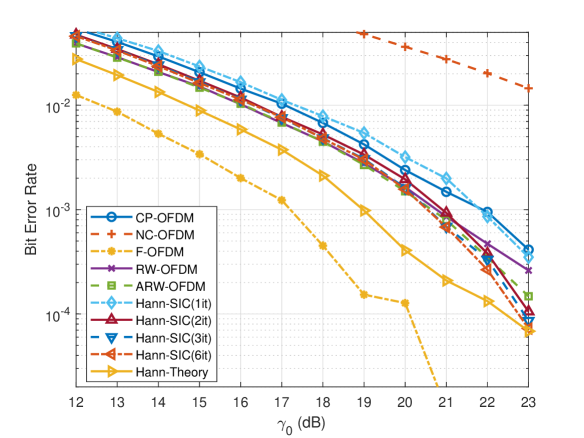
(a)

(b)

Figure 4: BERs of various transceivers for guard bands of $30\text{\,}\mathrm{kHz}$ between each user and (a) $10\text{\,}\mathrm{ns}$ and (b) $30\text{\,}\mathrm{ns}$ RMS delay spread.

Increasing the guard band drastically reduces the ACI present on the desired user’s band and narrows the gap between all algorithm as seen in Fig. 5. In Fig. 5a, compared to Fig. 4a, the increase in the guard band extended the orthogonal windowing algorithm’s lead against Hanning receivers beyond the target BER. However, it is seen that Hanning receivers, although requiring one more iteration, still outperform orthogonal windowing algorithms. Similarly as delay spreads elongate in Fig. 5b, the Hanning receiver’s advantage becomes more obvious with waterfall threshold moving further to lower SNRs compared to orthogonal windowing algorithms.

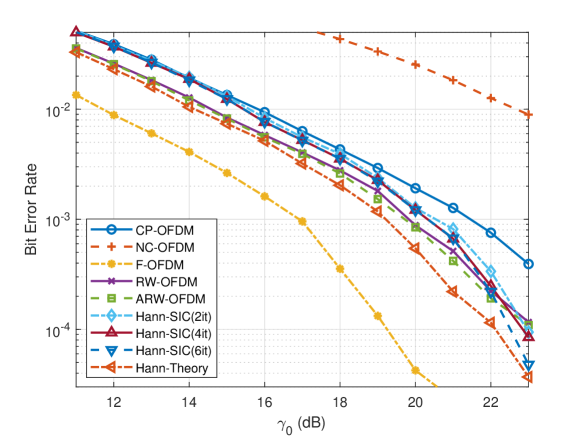
(a)

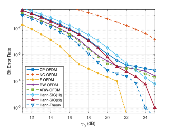
(b)

Figure 5: BERs of various transceivers for guard bands of $105\text{\,}\mathrm{kHz}$ between each user and (a) $10\text{\,}\mathrm{ns}$ and (b) $30\text{\,}\mathrm{ns}$ RMS delay spread.

Noting that the ACI sources utilize either transmitter windowed- (W-OFDM) or F-OFDM in other scenarios, both having superior out-of-band (OOB) emission suppression compared to NC-OFDM, the need to properly estimate and cancel the correction vector limits the BER performance of NC-OFDM. While F-OFDM has better BER performance beyond that theoretically achievable by Hanning receivers, Hanning receivers are used to resolve conventional CP-OFDM signals whereas F-OFDM can only be used to receive signals transmitted using a F-OFDM transmitter. Particularly, the filter lengths are $N/2+1$ per [39], the computational complexity of F-OFDM is $\left(N+L\right)\left(2N+4\right)$ real multiplications and $\left(N+L\right)\left(3N/2+2\right)$ real additions at both transmitter and receiver accordingly as filters consist of complex values. Similarly, the SSW RW-OFDM scheme described in [11] requires $6KD$ real multiplications and $4KD$ real additions to estimate received symbols. It is noteworthy that the complexity of F-OFDM scales on the order of FFT-size squared, whereas the complexity of windowing receivers scale linearly with the number of data-carrying subcarriers. Therefore, windowing receivers are particularly important for narrowband communications. The receiver computational complexity of Hanning receivers are accordingly compared with F-OFDM and RW-OFDM in Table II. Note that F-OFDM has symmetric computational complexity between the transmitting and receiving devices, whereas windowing receivers do not change the transmitter structure and do not cause any computational burden at the transmitting device. The window duration for RW-OFDM in short delay spread is considered as it makes more sense to apply RW-OFDM in that case.

TABLE II: Computational Complexity Comparison

Algorithm	Real Mult.	Real Add.
F-OFDM	2,248,992	1,685,648
RW-OFDM	3,672	2,448
Hann-SIC(1it)	3,224	984
Hann-SIC(2it)	3,632	1,356
Hann-SIC(3it)	4,040	1,728
Hann-SIC(4it)	4,448	2,100
Hann-SIC(6it)	5,264	2,844

V Conclusion

ACI is a critical problem in 5G and beyond scenarios due to the coexistence of OFDM based non-orthogonal signals. To tackle the ACI problem, we propose a novel Hann window function based low complexity receiver windowing method that is fully compatible with the frame structure of existing standards and needs no redundancy in the signal and no modifications on the transmitting devices. The proposed method improves the achievable capacity in the presence of high power non-orthogonal signals on adjacent channels when it is coupled with simple interference mitigation techniques. The proposed method allows superior ACI rejection and reducing guard bands without requiring extensions, and on the contrary, allows shortening the currently used extension for future higher mobility applications. Although the gap between prior art and the proposed methods widens with increasing delay spread and decreasing guard bands, the proposed methods outperform prior art in short delay spreads and large guard bands as well. This study paves the way towards future standard compliant ACI rejection research by showing gains of a simple receiver, inspiring sophisticated algorithms that outperform the presented by achieving performance bounds with less receiver complexity.

Berker Peköz (GS’15) received the B.S. degree (Hons.) in electrical and electronics engineering from Middle East Technical University, Ankara, Turkey in 2015, and the M.S.E.E. from University of South Florida, Tampa, FL, USA in 2017. He is currently pursuing the Ph.D. degree at University of South Florida, Tampa, FL, USA. His research is concerned with backward compatible standard compliant waveform design, and PHY algorithms and optimization thereof. Mr. Peköz is a member of Tau Beta Pi.

Zekeriyya Esat Ankaralı (GS’16) received the B.Sc. degree (Hons.) in control engineering from Istanbul Technical University, Istanbul, Turkey, in 2011, and the M.Sc. and Ph.D. degrees both in electrical engineering from the University of South Florida, Tampa, FL, USA, in 2013 and 2017, respectively. Since 2018, he has been with MaxLinear Inc., Carlsbad, CA, USA, as a staff communications systems engineer . His research interests are waveform design, physical layer security, and in vivo communications.

Selçuk Köse (S’10–M’12) received the B.S. degree in electrical and electronics engineering from Bilkent University, Ankara, Turkey, in 2006, and the M.S. and Ph.D. degrees in electrical engineering from the University of Rochester, Rochester, NY, USA, in 2008 and 2012, respectively. He was an Assistant Professor of Electrical Engineering at the University of South Florida, Tampa, FL, USA. He is currently an Associate Professor of Electrical and Computer Engineering at University of Rochester, Rochester, NY, USA. Dr. Köse is an Associate Editor of the World Scientific Journal of Circuits, Systems, and Computers and the Elsevier Microelectronics Journal.

Hüseyin Arslan (S’95-M’98-SM’04-F’15) received the B.S. degree in electrical and electronics engineering from Middle East Technical University, Ankara, Turkey in 1992, and the M.S. and Ph.D. degrees in electrical engineering from Southern Methodist University, Dallas, TX, USA in 1994 and 1998, respectively. From 1998 to 2002, he was with the research group of Ericsson Inc., Charlotte, NC, USA. He is currently a Professor of Electrical Engineering at the University of South Florida, Tampa, FL, USA, and the Dean of the College of Engineering and Natural Sciences at the İstanbul Medipol University, İstanbul, Turkey. Dr. Arslan is currently a member of the editorial board for the IEEE Communications Surveys and Tutorials and the Sensors Journal.

References

- [1] Z. Ankaralı, B. Peköz, and H. Arslan, “Flexible radio access beyond 5G: A future projection on waveform, numerology & frame design principles,” IEEE Access, vol. 5, no. 1, pp. 18 295–18 309, Dec. 2017.
- [2] 3GPP, “NR; Physical channels and modulation,” 3rd Generation Partnership Project (3GPP), Technical Specification (TS) 38.211, 01 2018, version 15.0.0.
- [3] X. Zhang, L. Zhang, P. Xiao, D. Ma, J. Wei, and Y. Xin, “Mixed numerologies interference analysis and inter-numerology interference cancellation for windowed OFDM systems,” IEEE Trans. Veh. Technol., vol. 67, no. 8, pp. 7047–7061, Aug. 2018.
- [4] R. Lupas and S. Verdu, “Near-far resistance of multiuser detectors in asynchronous channels,” IEEE Trans. Commun., vol. 38, no. 4, pp. 496–508, Apr. 1990.
- [5] J. Abdoli, M. Jia, and J. Ma, “Filtered OFDM: A new waveform for future wireless systems,” in Proc. 2015 IEEE 16th Int. Workshop Signal Process. Advances in Wireless Commun., Stockholm, SE, Jun. 2015, pp. 66–70.
- [6] C. Muschallik, “Improving an OFDM reception using an adaptive Nyquist windowing,” IEEE Trans. Consum. Electron., vol. 42, no. 3, pp. 259–269, Aug. 1996.
- [7] G. Turin, “An introduction to matched filters,” IRE Trans. Inform. Theory, vol. 6, no. 3, pp. 311–329, Jun. 1960.
- [8] I. P. Vaisband, R. Jakushokas, M. Popovich, A. V. Mezhiba, S. Köse, and E. G. Friedman, On-Chip Power Delivery and Management. Springer, Apr. 2016.
- [9] J. Gozalvez, “New 3GPP standard for IoT [mobile radio],” IEEE Veh. Technol. Mag., vol. 11, no. 1, pp. 14–20, March 2016.
- [10] E. Bala, J. Li, and R. Yang, “Shaping spectral leakage: A novel low-complexity transceiver architecture for cognitive radio,” IEEE Veh. Technol. Mag., vol. 8, no. 3, pp. 38–46, Sep. 2013.
- [11] E. Güvenkaya, A. Şahin, E. Bala, R. Yang, and H. Arslan, “A windowing technique for optimal time-frequency concentration and ACI rejection in OFDM-based systems,” IEEE Trans. Commun., vol. 63, no. 12, pp. 4977–4989, Dec. 2015.
- [12] C. F. Mecklenbrauker, A. F. Molisch, J. Karedal, F. Tufvesson, A. Paier, L. Bernado, T. Zemen, O. Klemp, and N. Czink, “Vehicular Channel Characterization and Its Implications for Wireless System Design and Performance,” Proc. IEEE, vol. 99, no. 7, pp. 1189–1212, Jul. 2011.
- [13] 3GPP, “Study on new radio access technology,” 3rd Generation Partnership Project (3GPP), Technical Report (TR) 38.912, 08 2017, version 14.1.0.
- [14] J. Wu and P. Fan, “A Survey on High Mobility Wireless Communications: Challenges, Opportunities and Solutions,” IEEE Access, vol. 4, pp. 450–476, 2016.
- [15] B. Peköz, S. Köse, and H. Arslan, “Adaptive windowing of insufficient CP for joint minimization of ISI and ACI beyond 5G,” in Proc. 2017 IEEE 28th Annu. Int. Symp. Personal, Indoor, and Mobile Radio Commun., Montreal, QC, Oct. 2017, pp. 1–5.
- [16] D. Slepian and H. O. Pollak, “Prolate spheroidal wave functions, fourier analysis and uncertainty - I,” Bell Syst. Tech. J., vol. 40, no. 1, pp. 43–63, Jan. 1961.
- [17] J. v. d. Beek and F. Berggren, “N-continuous OFDM,” IEEE Commun. Lett., vol. 13, no. 1, pp. 1–3, Jan. 2009.
- [18] R. B. Blackman and J. W. Tukey, “The measurement of power spectra from the point of view of communications engineering — Part I,” Bell Syst. Tech. J., vol. 37, no. 1, pp. 185–282, Jan. 1958.
- [19] K. Murota and K. Hirade, “GMSK modulation for digital mobile radio telephony,” IEEE Trans. Commun., vol. 29, no. 7, pp. 1044–1050, Jul. 1981.
- [20] F. J. Harris, “On the use of windows for harmonic analysis with the discrete Fourier transform,” Proc. IEEE, vol. 66, no. 1, pp. 51–83, Jan. 1978.
- [21] M. L. Honig, “Overview of multiuser detection,” in Advances in Multiuser Detection, M. L. Honig, Ed. Hoboken, N.J.: John Wiley & Sons, Inc., 2009, pp. 1–45.
- [22] M. J. Gans, “A power-spectral theory of propagation in the mobile-radio environment,” IEEE Trans. Veh. Technol., vol. 21, no. 1, pp. 27–38, Feb. 1972.
- [23] A. Kalakech, M. Berbineau, I. Dayoub, and E. P. Simon, “Time-Domain LMMSE Channel Estimator Based on Sliding Window for OFDM Systems in High-Mobility Situations,” IEEE Trans. Veh. Technol., vol. 64, no. 12, pp. 5728–5740, Dec. 2015.
- [24] R. W. Lucky, “Automatic equalization for digital communication,” Bell Syst. Tech. J., vol. 44, no. 4, pp. 547–588, Apr. 1965.
- [25] J.-v. d. Beek, O. Edfors, M. Sandell, S. K. Wilson, and P. O. Borjesson, “On channel estimation in OFDM systems,” in Proc. 1995 IEEE 45th Veh. Technol. Conf., vol. 2, Jul. 1995, pp. 815–819.
- [26] G. Huang, A. Nix, and S. Armour, “DFT-Based Channel Estimation and Noise Variance Estimation Techniques for Single-Carrier FDMA,” in Proc. 2010 IEEE 72nd Veh. Technol. Conf., Sep. 2010, pp. 1–5.
- [27] G. W. Stewart, “On scaled projections and pseudoinverses,” Linear Algebra Appl, vol. 112, pp. 189–193, Jan. 1989.
- [28] S. Vavasis, “Stable Numerical Algorithms for Equilibrium Systems,” SIAM J. Matrix Anal. Appl., vol. 15, no. 4, pp. 1108–1131, Oct. 1994.
- [29] P. Hough and S. Vavasis, “Complete Orthogonal Decomposition for Weighted Least Squares,” SIAM J. Matrix Anal. Appl., vol. 18, no. 2, pp. 369–392, Apr. 1997.
- [30] L. R. Kahn, “Ratio Squarer,” Proc. IRE, vol. 42, no. 11, p. 1704, Nov. 1954.
- [31] A. Barbieri, D. Fertonani, and G. Colavolpe, “Time-frequency packing for linear modulations: spectral efficiency and practical detection schemes,” IEEE Trans. Commun., vol. 57, no. 10, pp. 2951–2959, Oct. 2009.
- [32] 3GPP, “Study on new radio access technology Physical layer aspects,” 3rd Generation Partnership Project (3GPP), Technical Report (TR) 38.802, 09 2017, version 14.2.0.
- [33] ——, “NR; User Equipment (UE) radio transmission and reception; Part 1: Range 1 Standalone,” 3rd Generation Partnership Project (3GPP), Technical Specification (TS) 38.101-1, 01 2018, version 15.0.0.
- [34] ——, “Study on channel model for frequencies from 0.5 to 100 GHz,” 3rd Generation Partnership Project (3GPP), Technical Report (TR) 38.901, 01 2018, version 14.3.0.
- [35] R. C. Bose and D. K. Ray-Chaudhuri, “On a class of error correcting binary group codes,” Information and Control, vol. 3, no. 1, pp. 68–79, Mar. 1960.
- [36] A. Hocquenghem, “Codes correcteurs d’erreurs,” Chiffers, vol. 2, pp. 147–156, 1959.
- [37] W. W. Peterson, “On the weight structure and symmetry of BCH codes,” Hawaii Univ. Honolulu Dept. Electr. Eng., Honolulu, HI, Scientific-1 AD0626730, Jul. 1965.
- [38] R. M. Pyndiah, “Near-optimum decoding of product codes: block turbo codes,” IEEE Trans. Commun., vol. 46, no. 8, pp. 1003–1010, Aug. 1998.
- [39] f-OFDM scheme and filter design, 3GPP proposal R1-165 425, Huawei and HiSilicon, Nanjing, China, May 2016.