Temporal imaging for ultra-narrowband few-photon states of light

Abstract

Plenty of quantum information protocols are enabled by manipulation and detection of photonic spectro-temporal degrees of freedom via light-matter interfaces. While present implementations are well suited for high-bandwidth photon sources such as quantum dots, they lack the high resolution required for intrinsically narrow-band light-atom interactions. Here, we demonstrate far-field temporal imaging based on ac-Stark spatial spin-wave phase manipulation in a multimode gradient echo memory. We achieve spectral resolution of 20 kHz with MHz-level bandwidth and ultra-low noise equivalent to 0.023 photons, enabling operation in the single-quantum regime.

I Introduction

The temporal degree of freedom of both classical and quantum states of light enables or enhances a plethora of quantum information processing tasks Humphreys et al. (2014); Brecht et al. (2015); Reimer et al. (2016); Lu et al. (2019). In the development of quantum network architectures and novel quantum computing and metrology solutions, a significant effort has been devoted to quantum memories based on atomic ensembles, offering multi-mode storage and processing Pu et al. (2017); Parniak et al. (2017); Mazelanik et al. (2019); Seri et al. (2019), high efficiency Cho et al. (2016) or long storage-times Bao et al. (2012). Feasible implementations of protocols merging the flexibility of atomic systems and temporal processing capabilities inherently require an ability to manipulate and detect temporal photonic modes with spectral and temporal resolution matched to the narrow-band atomic emission. A versatile approach leveraging spectro-temporal duality, is to perform a frequency to time mapping – Fourier transform – in an analogy with far-field imaging in position-momentum space. To preserve quantum structure of non-classical states of light, systems relying on the concept of a time lens are employed Kolner and Nazarathy (1989); Zhu et al. (2013); Patera et al. (2018); however, presently existing physical implementations are well suited for high-bandwidth systems and involve either electro-optical phase modulation Kolner (1988); Grischkowsky (1974); Karpiński et al. (2017), sum-frequency generation Hernandez et al. (2013); Bennett and Kolner (2001); Bennett et al. (1994); Bennett and Kolner (1999); Agrawal et al. (1989) or four-wave mixing Kuzucu et al. (2009); Okawachi et al. (2009); Foster et al. (2008, 2009) in solid-state media. Figure 1 localizes the existing schemes in the bandwidth-resolution space. Methods relying on the time-lensing concept enable spectral shaping Li et al. (2015); Donohue et al. (2016); Lu et al. (2018), temporal ghost imaging Denis et al. (2017); Dong et al. (2016); Ryczkowski et al. (2017); Wu et al. (2019) and bandwidth matching Allgaier et al. (2017) for photons generated in dissimilar nodes of a quantum network. While those solutions offer spectral resolution suitable for high-bandwidth photons generated in spontaneous parametric down conversion (SPDC) or quantum-dot single-photon sources, their performance is severely limited in the case of spectrally ultra-narrow atomic emission ranging from few MHz to tens of kHz Zhao et al. (2014); Guo et al. (2017); Farrera et al. (2016), cavity coupled ions (below 100 kHz) Stute et al. (2012), cavity-enhanced SPDC designed for atomic quantum memories (below 1 MHz) Rambach et al. (2016), or optomechanical systems Hong et al. (2017); Hill et al. (2012).

In this Article we propose and experimentally demonstrate a novel, high-spectral-resolution approach to far-field temporal imaging which is inherently bandwidth-compatible with atomic systems, a regime previously unexplored as seen in Fig. 1, and works at the single-photon-level. This allows preservation of quantum correlations, manipulation of field-orthogonal temporal modes Brecht et al. (2015) and characterization of the time-frequency entanglement Mei et al. (2020) of photons from atomic emission. Our novel technique utilizes a recently developed spin-wave modulation method combined with unusual interpretation of Gradient Echo Memory (GEM) Hosseini et al. (2009) protocol to realize complete temporal imaging setup in a one physical system.

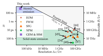
Figure 1: Temporal imaging state-of-the-art, characterized by temporal $\delta t$ and spectral $\delta\omega$ resolutions. Numerous implementations based on solid media (Electro-Optic Modulators (EOMS) - Foster et al. (2009); Kauffman et al. (1994); Azaña et al. (2004); Babashah et al. (2019), Four Wave Mixing (FWM) - Foster et al. (2008); Salem et al. (2009), Sum-frequency Generation (SFG) - Bennett and Kolner (1999); Suret et al. (2016), Cross Phase Modulation (XPM) - Mouradian et al. (2000)) are well suited for high bandwidth pico- or even femtosecond pulses, achieving spectral resolution no better than $1$ GHz, with time-bandwidth products ($\tau\mathcal{B}$) reaching $2\pi\times 2000$. Our system (Gradient Echo Memory and Spatial Spin-wave Modulation (GEM & SSM)) has $10^{6}$ times better spectral resolution $\delta\omega/2\pi\sim$20 kHz, maintaining good $\tau\mathcal{B}$, thus allowing exploration of previously unattainable region. The grayed region indicates unphysical area bounded by the Fourier limit $\tau\mathcal{B}/2\pi=1$.

II Principles of temporal imaging

Imaging systems generally consist of lenses interleaved with free-space propagation. Analogously, temporal imaging requires an equivalent of these two basic components. Involved transformations can be viewed in temporal or spectral domain separately, or equivalently by employing a spectro-temporal (chronocyclic) Wigner function defined as $W(t,\omega)=1/\sqrt{2\pi}\int_{-\infty}^{\infty}\mathrm{d}\xi A(t+\xi/2)A^{*}(t-\xi/2)\exp(-i\omega\xi)$, where $A(t)$ denotes the slowly varying amplitude of the signal pulse.

Temporal far-field imaging is typically achieved with a single time-lens preceded and followed by a temporal analog of free-space propagation. However, such a setup is equivalent to two lenses interleaved with a single propagation. In the Wigner function representation, combination of two temporal lenses with focal lengths $f_{\mathrm{t}}$, separated by a temporal propagation by the time $f_{\mathrm{t}}$, is described using a spectro-temporal equivalent of ray transfer matrix:

$$\negthickspace\negthickspace\begin{bmatrix}t^{\prime}\!\\ \frac{\omega^{\prime}}{\omega_{0}}\!\end{bmatrix}\!\negthickspace=\!\negthickspace\begin{bmatrix}1&0\\ -\frac{1}{f_{\mathrm{t}}}&1\end{bmatrix}\negthickspace\negthickspace\begin{bmatrix}1&f_{\mathrm{t}}\\ 0&1\end{bmatrix}\negthickspace\negthickspace\begin{bmatrix}1&0\\ -\frac{1}{f_{\mathrm{t}}}&1\end{bmatrix}\negthickspace\negthickspace\begin{bmatrix}t\!\\ \frac{\omega}{\omega_{0}}\!\end{bmatrix}\!\negthickspace=\!\negthickspace\begin{bmatrix}0&f_{\mathrm{t}}\\ -\frac{1}{f_{\mathrm{t}}}&0\end{bmatrix}\negthickspace\negthickspace\begin{bmatrix}t\!\\ \frac{\omega}{\omega_{0}}\!\end{bmatrix},$$ (1)

which represents a $\pi/2$ rotation in the phase space, exchanging temporal and spectral domains, where $\omega_{0}$ is the optical carrier frequency. To visualize this, in Fig. 2 (d) we present an equivalent of a cat state Wigner function (corresponding to sequence presented in Fig 3 (c)) undergoing these three subsequent transformations: (1) - time-lens, (2) - propagation, (3) - time lens.

To realize the time-lens with a focal length $f_{\mathrm{t}}$ one has to impose a quadratic phase $\exp[i\omega_{0}t^{2}/(2f_{\mathrm{t}})]$ on the optical pulse $A(t)\to A(t)\exp[i\omega_{0}t^{2}/(2f_{\mathrm{t}})]$, where $\omega_{0}$ is the optical carier frequency. In the language of Wigner functions, this transformation can be written as $W(t,\omega)\to W(t,\omega^{\prime})$ with $\omega^{\prime}=\omega-\omega_{0}t/f_{\mathrm{t}}$. This corresponds to adding to the pulse a linear chirp $\omega(t)=\omega_{0}+\alpha t$. Typically, such a transformation is achieved by directly modulating the signal pulse using electro-optic modulators Foster et al. (2009); Kauffman et al. (1994); Azaña et al. (2004); Babashah et al. (2019).

The analog of free-space propagation can be understood as a frequency-dependent delay applied to an optical pulse. In the language of the Wigner function, the transformation takes a form $W(t,\omega)\to W(t^{\prime},\omega)$ with $t^{\prime}=t+f_{\mathrm{t}}\omega/\omega_{0}$. Equivalently, a pulse with spectral amplitude $\widetilde{A}(\omega)=\mathcal{F}_{t}[A(t)](\omega)$ needs to acquire a parabolic spectral phase $\widetilde{A}(\omega)\to\widetilde{A}(\omega)\exp[-i(f_{\mathrm{t}}/\omega_{0})\omega^{2}]$. Commonly, such an operation is realized directly by propagation in dispersive media Karpiński et al. (2017) or by employing a pulse stretcher/compressor.

III Temporal imaging using GEM and SSM

In our technique we employ the atomic ensemble to process stored light and implement the temporal imaging operations during storage or light-atom mapping. The optical signal amplitude $A(t)$ is mapped onto the atomic coherence in a $\Lambda$ type system built of three atomic levels $|g\rangle$, $|h\rangle$ and $|e\rangle$ (see Fig. 2 (a)). The mapping process employs a strong control field to make the atoms absorb the signal field and generate an atomic coherence $\rho_{hg}$ commonly called a spin-wave (SW). During the mapping (and re-mapping) process the atoms are kept in a magnetic field gradient, which constitutes the basis of the GEM Hosseini et al. (2009), providing linearly changing Zeeman splitting between the $|h\rangle$ and $|e\rangle$ levels along the atomic cloud. This means that the signal-control two-photon interaction happens with a spatially dependent two-photon detuning $\delta$, and only atoms contained in a limited volume will interact efficiently with signal light of a specific frequency. Therefore, distinct spectral components of signal light $\widetilde{A}(\omega)$ are mapped onto different spatial components of the atomic coherence $\rho_{hg}(z)\propto\widetilde{A}(\beta z)$ Hosseini et al. (2009); Sparkes et al. (2013) (see Fig. 2 (b)) and vice versa, where $\beta$ denotes the gradient of the Zeeman shift along the propagation ($z$) axis.

The temporal equivalent of free space propagation is realized thanks to this spectro-spatial mapping, characteristic of the GEM. Spatially-resolved phase modulation of a SW stored in the memory is equivalent to imposing a spectral phase profile onto the signal. Thus, by imposing onto the SWs a parabolic spatial phase $\exp[-if_{\mathrm{t}}/(2\omega_{0})\beta^{2}z^{2}]$ we implement the temporal analog of free-space propagation. This operation is implemented using the spatially-resolved ac-Stark shift induced by an additional far-detuned and spatially-shaped laser beam – a technique we call spatial spin-wave modulation (SSM) Leszczyński et al. (2018); Parniak et al. (2019); Mazelanik et al. (2019); Lipka et al. (2019).

To make the time-lens we utilize the fact that the SW is created in coherent two-photon absorption, thus it reflects the temporal phase difference between the control and signal field. This means, that chirping the signal field is equivalent to chirping the control field, as only the two-photon detuning $\delta$ is crucial here. Hence, by changing the control field frequency, we make the two-photon detuning linearly time dependent $\delta=\alpha t$ and impose the desired quadratic phase during the interaction time. This way the time-lens is realized at the light-SW mapping stage without affecting the signal field directly. Yet, as we chose the single-photon detuning $\Delta\gg\delta$ residual modulation of the coupling efficiency is negligible as $\Delta+\alpha t\approx\Delta$.

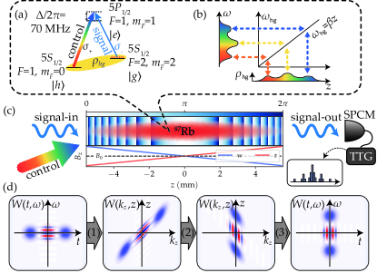
Figure 2: (a) Light-atom interface. Chirped control field simultaneously allows mapping of the signal optical field onto the atomic coherence $\rho_{hg}$ and realizes the temporal lens. (b) Projection of signal spectral components onto atomic coherence spatial components in GEM with Zeeman splitting gradient $\beta$. (c) During the writing process atoms are placed in a negative magnetic field gradient along the cloud (w). When the writing finishes, the spatial phase of the atomic coherence is modulated with a parabolic Fresnel profile which realizes a temporal equivalent of free-space propagation. Finally, the gradient is switched to positive (r) and the coherence is converted back to light which is further registered with Single-Photon-Counting-Module (SPCM) connected to the Time Tagger (TTG). (d) Evolution of the spectro-temporal Wigner function on subsequent stages of far-field temporal imaging: (1) – time-lens, (2) – free-space propagation, (3) – time-lens. The complete transformation effectively rotates the initial Wigner function of two pulses (equivalent to a Wigner function of a cat state in phase space) by $\pi/2$ as given by Eq. 1.

Finally, sending a signal field $A(t)$ through a lens-propagation-lens temporal imaging system, the output amplitude is proportional to $\widetilde{A}\left(\alpha t\right)$. In practice, however, the finite size of the atomic cloud must be taken into account making the output amplitude proportional to $\left(\left[\widetilde{A}(\alpha t)\exp[-i(\alpha/2)t^{2}]\right]*\zeta(t)*\zeta(t)\right)\exp[i(\alpha/2)t^{2}]$, where $\zeta(t)=\mathcal{F}_{\omega}[\eta_{0}(\omega)](t)$ is the Fourier transform of the inhomogeneously broadened absorption efficiency spectrum $\eta_{0}(\omega)$ determined by the atomic density distribution and field gradient $\beta$, and $*$ symbolizes convolution.

In a typical regime of operation we select the chirp $\alpha\ll(\beta L)^{2}$ to always contain the entire spectrum of the pulse within the atomic absorption bandwidth $\mathcal{B}\approx\beta L$. The resolution in this regime is limited by the decoherence of spin-waves caused by the control beam of the light-atom interface and is given by the inverse of the atomic coherence lifetime $\delta\omega/2\pi=0.78/\tau$ (see Supplement 1 for derivation of the prefactor), where $1/\tau=\Gamma\Omega^{2}/(4\Delta^{2}+\Gamma^{2})$ and $\Gamma$ is the decay rate of the $|e\rangle$ state and $\Omega$ is the Rabi frequency at the $|h\rangle\rightarrow|e\rangle$ transition.

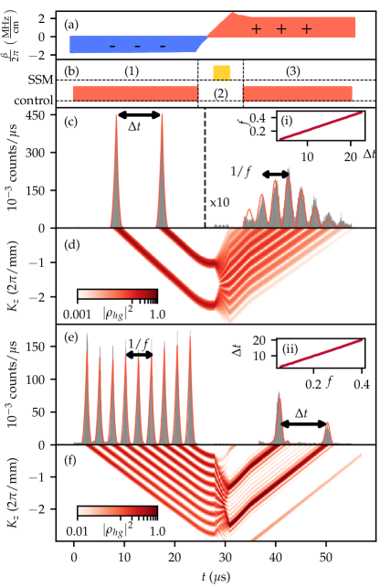
Figure 3: Experimental sequence for temporal imaging. (a) Time-trace of the Zeeman shift gradient $\beta$ used in GEM protocol, allowing two-directional mapping of signal frequencies to distinct positions in the atomic cloud. (b) Control field (red) and SSM (yellow) laser pulse sequence divided into three stages corresponding to lens-propagation-lens operations. The lens (1) is implemented during the GEM writing process by a chirped control field. (2) The 3 $\mu$s-long SSM laser pulse imprints a parabolic phase profile onto the stored atomic coherence which realizes the spectro-temporal free-space propagation. During this stage the magnetic field gradient is reversed, allowing re-mapping the coherence to light. (3) Finally, the control field is turned on and the coherence is read-out from the memory. Chirping the control field would implement the second lens. However, for simplicity, the control field is no longer chirped as the imposed phase would not be registered by the SPCM. (c,e) Example results, for two pulses or a sine-wave as inputs, respectively. Gray bins represent single photon counts. Red line corresponds to the numerical simulations. (d,f) Normalized modulus square of atomic coherence in Fourier space. The insets (i,ii) show experimentally obtained linear dependency of the time delay $\Delta t$ (in $\mu\mathrm{s}$) on the signal modulation frequency $f$ (in MHz) defined on panels (c,e).

IV Experiment

The core of our setup is a GEM based on a cold ⁸⁷Rb atomic ensemble trapped in a magneto-optical trap (MOT) over 1-cm-long pencil-shaped volume. After the MOT release, all atoms are optically pumped to the $|g\rangle=5\mathrm{S}_{1/2}$, $F=2$, $m_{F}=2$ state. The ensemble optical depth reaches $\mathrm{{OD}}\sim 70$ at the $|g\rangle\rightarrow|e\rangle=5P_{1/2}$, $F=1$, $m_{F}=1$ transition. As depicted in Fig. 2(a), we employ the $\Lambda$ system to couple light signal and atomic coherence (spin-waves). The interface consists of a $\sigma_{+}$ polarized strong control laser blue-detuned by $\Delta=2\pi\times 70$ MHz from the $|h\rangle=5S_{1/2}$, $F=1$, $m_{F}=0\rightarrow|e\rangle$ transition and a weak $\sigma_{-}$ polarized signal laser at the $|g\rangle\rightarrow|e\rangle$ transition, approximately at the two-photon resonance $\delta\approx 0$. The gradient $\beta$ of the Zeeman splitting along the $z$ axis during signal-to-coherence conversion is generated by two rounded-square shaped coils connected in opposite configuration (see Supplement 1 for details). The SSM scheme facilitates manipulation of the spatial phase of stored spin-waves via off-resonant ac-Stark shift by illuminating the atomic cloud with a spatially shaped strong $\pi$-polarized beam, 1 GHz blue-detuned from the $5S_{1/2}$, $F=1\rightarrow 5P_{3/2}$ transition. The signal emitted in $|g\rangle\rightarrow|e\rangle$ transition is filtered using Wollaston polarizer and an optically-pumped atomic filter, to be finally registered on a Single Photon Counting Module (SPCM). We finally register only $0.023$ noise counts on average per $\tau$-long detection window (see Supplement 1 ).

In Fig. 3 we present exemplary measurements performed with our setup. Panel (a) shows the time trace of the Zeeman shift gradient set initially to $\beta=-2\pi\times 1.7$ MHz/cm. In panel (b) we provide the control and SSM laser sequence divided into stages corresponding to subsequent implementations of lens-propagation-lens operations. (1) First, a strong control field (Rabi frequency $\Omega=2\pi\times 4.7$ MHz) is used to map a weak ($\bar{n}=2.8$) signal pulse with temporal amplitude $A(t)$ to the atomic coherence. The control beam is chirped with an acousto-optic modulator (AOM) to have a time-dependent frequency of $\omega(t)=\omega_{0}+\alpha t$, with $\alpha=2\pi\times 0.04$ MHz/$\mu$s. This implements a time-lens with focal length $f_{\mathrm{t}}=9.6\times 10^{3}$ s. (2) Next, within 7 $\mu$s the gradient $\beta$ is switched to opposite value and a parabolic Fresnel phase profile $\exp[-i\beta^{2}/(2\alpha)z^{2}]$ (as depicted in Fig. 2(c)) is imprinted onto stored atomic coherence by the 3 $\mu$s long SSM laser pulse. The linear gradient of magnetic field only shifts atomic coherence in the Fourier domain, therefore phase modulation can be done simultaneously with $\beta$ reversing. (3) Finally, the control field is turned on and the coherence is converted back to light. For simplicity, during GEM readout the control field is no longer chirped as the imposed phase would not be registered by the the SPCM (see Supplement 1 for details).

Figure 3(c-f) portrays experimental results for two types of the input signal: (c,d) two peaks and (e,f) sine-wave-like waveform. Red solid lines corresponds to the full light-atoms interaction simulation (see Supplement 1 for details). The density maps (d,f) below each time trace (c,e) show simulated evolution of the atomic coherence during the experiment. For both input signal shapes the measured efficiency amounts to about 7%. The insets (i,ii) show experimentally obtained linear relationship between time delay $\Delta t$ and the signal modulation (temporal fringes) frequency $f$ defined in panels (c,e).

We attribute the residual mismatch between experimental results and theoretical predictions to imperfect linearity of magnetic field gradient, decoherence caused by ac-Stark modulation and a simplification of the atomic density distribution in the simulation. However, for both exemplary measurements we can still observe a good agreement with the theory. Notably, the simulations use independently calibrated parameters, with only the input photon number adjusted for the specific measurements.

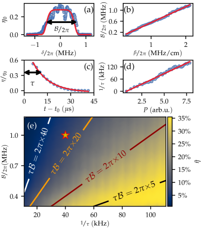
Figure 4: Characterization and tuning of bandwidth and resolution. (a) Efficiency spectral profile $\eta_{0}(\omega)$ as a function of the two-photon detuning $\delta=\omega-\omega_{0}$ for a chosen time-bandwidth product $\tau\mathcal{B}=2\pi\times 13$ with bandwidth $\mathcal{B}$ defined as FWHM of $\eta_{0}(\omega)$. The red line corresponds to a super-Gaussian approximation of the atom concentration used in the simulation. (b) Dependence of the bandwidth $\mathcal{B}$ as a function of the Zeeman splitting gradient $\beta$. Red line is a linear fit to the data. (c) Time evolution of the GEM efficiency due to incoherent scattering caused by the coupling field. The characteristic decay time $\tau$ obtained from exponential fit (red line) limits the effective resolution $\delta\omega/2\pi=0.78/\tau$ (here $\tau=10\ \mu\mathrm{s}$). (d) Dependence of $1/\tau$ as a function of the coupling field power $P\propto|\Omega|^{2}$, along with linear fit (red line). (e) Calculated map of the average efficiency $\bar{\eta}$ for varying bandwidth $\mathcal{B}$ and decay time $\tau$. The efficiency for a given time-bandwidth product $\tau\mathcal{B}$ is approximately constant as expected. The star indicates the point of operation where the exemplary measurements (Fig. 3) were performed.

V Time-bandwidth characterization

Figures of merit characterizing our device are bandwidth, resolution and efficiency. Those parameters are related by a formula for GEM efficiency Sparkes et al. (2013) which for atoms uniformly distributed over the length $L$ becomes $\omega$-independent and can be approximated as

$$\eta_{0}=\left[1-\exp\left(-2\pi\frac{\mathrm{OD}}{\tau\mathcal{B}}\right)\right]^{2},$$ (2)

where OD is the optical depth of the ensemble for $\Delta=0$. Equation 2 indicates that increased bandwidth or resolution results in a drop in efficiency. In a realistic scenario atoms are non-uniformly distributed over the cloud and thus different spectral components of the input field experience different values of OD, especially at the edges of the atomic cloud. This makes the efficiency $\eta_{0}$ frequency-dependent and leads to an operational definition of the bandwidth $\mathcal{B}$ as the FWHM of the $\eta_{0}(\omega)$ profile as depicted in Fig. 4(a). Additionally, due to the decoherence induced by the coupling field during the write (and read) process, the efficiency decays exponentially in time: $\eta=\eta_{0}\Theta(t)\exp(-t/\tau)$, as illustrated in Fig. 4(c). Therefore, to account for spectro-temporal dependencies, we introduce a time-frequency averaged efficiency:

$$\bar{\eta}=\frac{1}{2\tau\mathcal{B}}\int_{-\mathcal{B}/2}^{\mathcal{B}/2}\int_{0}^{2\tau}\eta(t,\omega)\mathrm{d}t\mathrm{d}\omega=\frac{e^{2}-1}{2e^{2}\mathcal{B}}\int_{-\mathcal{B}/2}^{\mathcal{B}/2}\eta_{0}(\omega)\mathrm{d}\omega.$$ (3)

Figure 4(e) illustrates measured values of $\bar{\eta}$ for different $\mathcal{B}$ and $\tau$. The map is built from separate measurements of $\eta_{0}(\omega)$ (Fig. 4(a)) and $\tau$ (Fig. 4(c)) for different Zeeman shift gradient $\beta$ (Fig. 4(b)) and control laser power $P\propto|\Omega|^{2}$ (Fig. 4(d)). The parameters extracted from Fig. 4(a-d) are then combined to give value of $\bar{\eta}$ for each $(\tau(P),\mathcal{B}(\beta))$ point. As expected from Eq. 2, we see a clear trade-off between the time-bandwidth product $\tau\mathcal{B}$ and the average efficiency $\bar{\eta}$. Conversely, requiring a higher number of distinguishable frequency (or time) bins leads to a lower efficiency. Yet, with $\sim 20$% mean efficiency we obtain $\tau\mathcal{B}=2\pi\times 10$ that simultaneously yields 100 kHz resolution and 1 MHz bandwidth. One may also choose to maximize $\tau\mathcal{B}$ to reach $2\pi\times 40$, with mean efficiency $\sim 4\%$. Notably, as the efficiency $\eta_{0}$ saturates for large OD, for systems with ultra-high optical depth the time-bandwidth product could reach significantly higher values while maintaining near-unity efficiency for many bins.

VI Conclusions

In summary, we have introduced and experimentally demonstrated a novel high-resolution (ca. 20 kHz) far-field imaging method suitable for narrow-band atomic photon sources – a region previously unattainable. The device may also serve as a single-photon-level ultra-precise spectrometer for atomic emission, enabling characterization of spectro-temporal high-dimensional entanglement generated with atoms. In general, while temporal domain characterization and manipulation at the single-photon level is already indispensable in numerous quantum information processing tasks, quantum networks architectures and metrology, our device will allow those techniques to enter the ultra-narrow bandwidth domain. Our method utilizes a multi-mode gradient echo memory (GEM) along a recently developed processing technique – spatial spin-wave modulator (SSM) Parniak et al. (2019); Mazelanik et al. (2019); Lipka et al. (2019) – enabling nearly arbitrary manipulations on light states stored in GEM. We envisage that with improvement of the magnetic field gradient the GEM bandwidth can reach dozens of MHz opening new ranges of applications such as solid-state quantum memories Hedges et al. (2010) and color centers Jeong et al. (2019). Furthermore, our approach utilizes a quantum memory previously demonstrated Parniak et al. (2017); Mazelanik et al. (2019) to operate with quantum states of light, and maintains the ultra low level of noise, creating novel possibilities in temporal and spectral processing of narrow-band atomic-emission quantum states of light. Our technique applied to systems with higher absorption bandwidth Saglamyurek et al. (2018) or optical depth Cho et al. (2016) can bridge the bandwidth gap to enable hybrid solid-state–atomic quantum networks operating using the full temporal-spectral degree of freedom.

Funding.

MNiSW (DI2016 014846, DI2018 010848); National Science Centre (2016/21/B/ST2/02559, 2017/25/N/ST2/01163, 2017/25/N/ST2/00713); Foundation for Polish Science (MAB 4/2017 "Quantum Optical Technologies"); Office of Naval Research (N62909-19-1-2127).

Acknowledgments.

We thank K. Banaszek for the generous support and M. Jachura for insightful discussion. M.P. was supported by the Foundation for Polish Science via the START scholarship. A.L. and M.M. contributed equally to this work. The "Quantum Optical Technologies ” project is carried out within the International Research Agendas programme of the Foundation for Polish Science co-financed by the European Union under the European Regional Development Fund.

M.M. and A.L. contributed equally to this work.

Supplementary material

Light-atoms interaction

To describe interaction between light and atomic coherence we use three level atom model with adiabatic elimination. The most comfortable coordinate system runs in time with beam $t\to t+z/c$. We explicitly make the control Rabi frequency $\Omega(t)$ time-dependent, as this is directly controlled in the experiment. Notably, $\Omega(t)$ represents the slowly-varying amplitude of this control field. Furthermore, we write the equations in terms of demodulated zero-spatial-frequency coherence $\check{\rho}_{hg}(z,t)=\rho_{hg}(z,t)e^{iK_{z0}z-i\Delta_{\mathrm{{HFS}}}t}$, where $\rho_{hg}(z,t)$ is the actual ground-state coherence, $\Delta_{\mathrm{{HFS}}}\approx 2\pi\times 6.8\ \mathrm{{GHz}}$ is the hyperfine splitting between levels $|g\rangle$ and $|h\rangle$ and $K_{z0}=\sqrt{{\omega_{0}^{2}/c^{2}-k_{x}^{2}-k_{y}^{2}}}-\omega_{C}/c$ ($\omega_{C}$ - coupling field frequency, $k_{x},\ k_{y}$- transverse spatial components of the signal beam with respect to the coupling beam; for our case $k_{y}=0$ and $ck_{x}/\omega_{0}\approx 8\ \mathrm{mrad}$). Then, the light-coherence evolution is given by following coupled equations written in the frame of reference co-moving with the optical pulse:

$$\frac{\partial\check{\rho}_{hg}(z,t)}{\partial t}=\frac{i}{\hbar}\frac{\Omega^{*}(t)dA(z,t)}{4\Delta-2i\Gamma}-\frac{1}{2\tau}\check{\rho}_{hg}(z,t)+i\delta_{\mathrm{tot}}(z,t)\check{\rho}_{hg}(z,t),$$ (S1)

$$\frac{\partial A(z,t)}{\partial z}=-i\frac{\hbar\Omega(t)\check{\rho}_{hg}(z,t)/d+A(z,t)}{2\Delta+i\Gamma}\frac{\Gamma}{2}gn(z),$$ (S2)

where $1/(2\tau)=|\Omega(t)|^{2}\Gamma/(8\Delta^{2}+2\Gamma^{2})$ is decoherence caused by radiative broadening, $\delta_{\mathrm{tot}}=\delta_{0}+\delta_{\mathrm{acS}}+\delta_{\mathrm{SSM}}+\delta_{Z}$ is total two-photon detuning including ac-Stark shift caused by control beam $\delta_{\mathrm{acS}}=|\Omega(t)|^{2}\Delta/(4\Delta^{2}+\Gamma^{2})$, SSM and spatially varying Zeeman shift $\delta_{Z}=\mu_{0}g_{F}mB_{0}+\beta z$ , with $F=2$, $m=2$ and $g_{F=2}=1/2$ , caused by linearly varying external magnetic field $B=B_{0}+\frac{\beta}{\mu_{0}}z$, where $\mu_{0}$ is the Bohr magneton. The atomic concentration is denoted by $n(z)$ and we define the ensemble optical depth as $\mathrm{OD}=\intop gn(z)\mathrm{d}z$. In practice the value of $\delta_{0}$ is chosen to cancel out the light shift caused by the control field: $\delta_{0}=-\delta_{\mathrm{acS}}$.

Spectral resolution

The spectral resolution of the device is limited by finite duration $T$ of the measurement window combined with the exponential decay of the atomic coherence caused by the control field. One could consider that upper limit for $T$ is given by combination of the bandwidth $\mathcal{B}$ and the control field chirp $\alpha$ by $T_{\mathrm{max}}=\mathcal{B}/\alpha$ as for $\alpha T>\mathcal{B}$ a monochromatic input field $\tilde{A}(\omega)=\delta(\omega)$ lies outside the inhomogeneously broadened absorption spectrum. However, in the usual operation regime we set $\alpha\ll\mathcal{B}^{2}$ and to maintain high initial efficiency we always have $\tau<T_{\mathrm{max}}$. In this regime the finite atomic coherence lifetime $\tau$ limits the available measurement time $T$ which we set to be $T=\tau$ to maintain high overall efficiency $\bar{\eta}$. To estimate the resolution accounting for both $\tau$ and $T$ we calculate the power spectrum of a monochromatic input pulse with exponentially decaying amplitude $A(t)=(\Theta(t)-\Theta(t-\tau))\exp(-\frac{t}{2\tau})$:

$$|\tilde{A}(\omega)|^{2}\propto\frac{1+e-2\sqrt{e}\cos(\tau\omega)}{4\tau^{2}\omega^{2}+1},$$

and define the spectral resolution $\delta\omega$ as FWHM of the power spectrum $|\tilde{A}(\omega)|^{2}$. We numerically find $\delta\omega/2\pi\approx 0.78/\tau$.

Group-delay dispersion estimate

By imposing the parabolic phase shift onto the atomic ensemble, we imitate temporal imaging setups that use group-delay dispersion in chirped fiber Bragg gratings (CFBG), or just fibers, to achieve large group delays. The temporal propagation length we achieve in our setup amounts to $f_{t}=9600\ \mathrm{{s}}$ which corresponds to a GDD of $25\ \mu\mathrm{{s}}^{2}$ over our 1 MHz bandwidth. To achieve such GDD, one would need $10^{12}\ \mathrm{{km}}$ of typical telecom fiber (GDD $25\ \mathrm{{ps}^{2}/km}$) or billions of commercially available CFBGs (GDD $\sim 10^{4}\ \mathrm{{ps}^{2}}$).

Simplified protocol

In the main Article we mentioned that in practice the temporal far-field imaging sequence we do not implement the chirp at readout, as it would not change the final intensity. While this is true in the ideal case, here we also want to argument that in our particular implementation it bear almost no difference. In particular, then only reason the difference may arise is a relative change in the single-photon detuning $\Delta$. Here we simulate the protocol with and without the chirp and in Fig. S1 we observe that the difference is minimal, staying always below 1%.

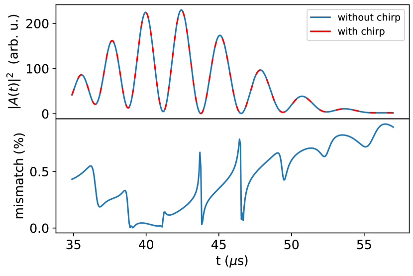
Figure S1: Simulated comparison of the output signal, as in Fig. 3(c) of the main Article with and without the chirp of the readout field. We observe no more than 1% difference, varying that omitting the final chirp for the purpose of observing proper intensity profile at the output is well justified.

Experimental setup details

Magnetic field

To determine the quantization axis the atomic cloud is kept in external constant $\sim 1$ G magnetic field along the cloud, generated by external Helmholtz coils. The gradient of magnetic field for GEM is generated by a pair of rounded square-shaped coils in opposing configuration connected in series. The coils are made of 9 turns of copper wire wound over a base with a side length $d=10$ cm. The separation between the coils is $L=17$ cm. This configuration provides almost linear magnetic field gradient of value 0.08 G/A/cm over the 10 mm long cloud. The coils current and thus the gradient can be quickly switched to the opposite value using an electronic switch capable of connecting either constant current source (typ. 15A) in either direction or providing 160V for fast current reversal. This is accomplished using MOSFETs in H-bridge topology. The high switching speed (4.3 A/$\mu$s corresponding to $0.35$ G/cm/$\mu$s) equals 160 V divided by inductance of the coils.

The instantaneous current in the coils is measured using LEM-LA 100-P current transducer with sub $\mu$s response time. The apparent overshoot after the current reversal is in fact a start of a combination of oscillation of LC circuit formed by the coils inductance and parasitic capacitance of the switch and an exponential decay of the current to a new steady state value. When the control field is not applied the value of the magnetic field gradient $\beta$ controls only the speed of shifting the atomic coherence in the $K_{z}$ space. Therefore, by applying the control after a short delay from the end of the switching state (when the overshoot is mostly present) we avoid the unwanted effect of readout efficiency change due to different instantaneous bandwidth $\mathcal{B}$. The residual variation of $\beta$ during the readout process slightly affects the temporal profile of readout speed, which manifests as a chirp of the expected intensity oscillations of the output signal, as in Fig. 3(d) of the Article.

The magnetic gradient overshoot is in reality much smaller than estimated from the instantaneous current. We attribute this to eddy currents created in the metal parts of the magneto-optical trap apparatus occurring during switching of the coils which virtually compensate the amount of gradient change due to the overshoot.

Filtering system and noise characterization

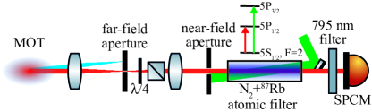
Figure S2: Filtering setup. The signal separated from the coupling laser light using a sequence of far field apertures, Wollaston polarizer, near field aperture, optically pumped atomic filter and interference filter. Transmission of the signal photons through this system amounts about 60%.

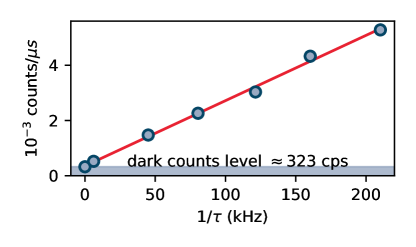
Figure S3: SPCM noise photons count rate versus decay rate of atomic coherence. The slope of the fitted line amounts to 0.023 and can be interpreted as average number of noise photons registered during readout process.

To minimize the noise we need to efficiently filter signal photons from the control beam and other noise. For this purpose, we have built a multi-stage filtering system (Fig. S2). Firstly, we filter most of control beam photons using far field aperture. Next, we use the fact that they have orthogonal polarization to the signal photons and we filter them using quarter-wave plate and Wollaston polarizer. After that we use near field aperture to remove photons scattered in other parts of MOT. Later, the glass cell containing Rubidium-87 pumped to $5S_{1/2},F=1$ state with 780 nm laser and buffer gas (nitrogen) is used to filter out stray control beam light while preserving the multimode nature of our device as compared to the cavity based filtering. Finally we use a 795 nm interference filter to remove other frequency photons, coming mainly from the filter pump.

To estimate the amount of noise present in our experiment we use the same experimental sequence as in Fig. 3 but without any optical field at the input. We perform the experiment for different values of the control laser power $P$ and calculate the noise count rate for each point. In Figure S3 we present measured noise count rate as a function of atomic coherence decay rate $1/\tau$, which is proportional to the power of the control beam $P$ (see Fig. 4(d) in the Article). The slope of the fitted line can be interpreted as average number of noise photons registered during the typical $\tau$-long readout process. Note that as we increase the coupling laser intensity, we register more noise photons yet during a shorter window. This gives us a constant mean photon number per readout. Thanks to our filtering system we achieved the value of $\bar{{n}}_{\mathrm{{noise}}}=0.023$ which means, that we register approximately 1 noise photon per 40 single experiments. Simultaneously, the transmission of the signal photons amounts to about 60%, while the detection efficiency is $\sim$ 65%. With a typical memory process efficiency of 25%, we obtain noise per single photon sent to the device $\mu_{1}=0.23$, which corresponds to $\mu_{1}=0.016$ per single mode (i.e. in a single temporal mode storage experiment).The main limitation is still filtering of coupling light, as witnessed by removing the atomic ensemble and still observing the same noise level. That could be improved further by coupling the signal to a single-mode fibre or using more efficient filtering.

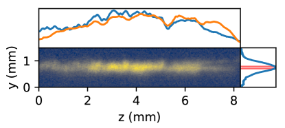
Figure S4: Fluorescence image of atomic cloud from the side. Center blue lines corresponds to its integrals along $y$ and $z$ axis. Red area, to the right marks the part of atomic cloud illuminated with signal laser. The orange line above presents concentration distribution along the $z$ axis corresponding to the spectral profile in presence of magnetic field gradient.

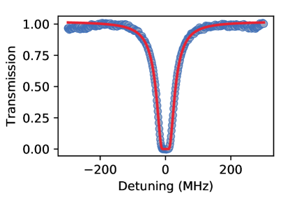
Figure S5: Single photon absorption profile of the signal laser. Fitted red line corresponds to OD=76.

Optical depth

Figure S4 shows the image of atomic cloud from the side. Atoms are formed into pencil shape area with diameter of about 0.5 mm. The signal laser diameter amounts to about 0.1 mm and illuminates the middle of the atomic cloud, where the optical depth is the highest. Figure S5 presents single photon absorption profile of the signal. Fitting the saturated Lorentz profile, we estimated that optical depth amounts to about 76.

References

- Humphreys et al. (2014) P. C. Humphreys, W. S. Kolthammer, J. Nunn, M. Barbieri, A. Datta, and I. A. Walmsley, Phys. Rev. Lett. 113, 130502 (2014), arXiv:1405.5361 .
- Brecht et al. (2015) B. Brecht, D. V. Reddy, C. Silberhorn, and M. G. Raymer, Physical Review X 5, 041017 (2015), arXiv:1504.06251 .
- Reimer et al. (2016) C. Reimer, M. Kues, P. Roztocki, B. Wetzel, F. Grazioso, B. E. Little, S. T. Chu, T. Johnston, Y. Bromberg, L. Caspani, D. J. Moss, and R. Morandotti, Science 351, 1176 (2016).
- Lu et al. (2019) H.-H. Lu, J. M. Lukens, B. P. Williams, P. Imany, N. A. Peters, A. M. Weiner, and P. Lougovski, npj Quantum Inf. 5, 24 (2019), arXiv:1809.05072 .
- Pu et al. (2017) Y. F. Pu, N. Jiang, W. Chang, H. X. Yang, C. Li, and L. M. Duan, Nat. Commun. 8, 15359 (2017), arXiv:1707.07267 .
- Parniak et al. (2017) M. Parniak, M. Dąbrowski, M. Mazelanik, A. Leszczyński, M. Lipka, and W. Wasilewski, Nat. Commun. 8, 2140 (2017), arXiv:1706.04426 .
- Mazelanik et al. (2019) M. Mazelanik, M. Parniak, A. Leszczyński, M. Lipka, and W. Wasilewski, npj Quantum Inf. 5, 22 (2019), arXiv:1808.00927 .
- Seri et al. (2019) A. Seri, D. Lago-Rivera, A. Lenhard, G. Corrielli, R. Osellame, M. Mazzera, and H. de Riedmatten, Phys. Rev. Lett. 123, 080502 (2019), arXiv:1902.06657 .
- Cho et al. (2016) Y.-W. Cho, G. T. Campbell, J. L. Everett, J. Bernu, D. B. Higginbottom, M. T. Cao, J. Geng, N. P. Robins, P. K. Lam, and B. C. Buchler, Optica 3, 100 (2016), arXiv:1601.04267 .
- Bao et al. (2012) X. H. Bao, A. Reingruber, P. Dietrich, J. Rui, A. Dück, T. Strassel, L. Li, N. L. Liu, B. Zhao, and J. W. Pan, Nat. Phys. 8, 517 (2012), arXiv:1207.2894 .
- Kolner and Nazarathy (1989) B. H. Kolner and M. Nazarathy, Opt. Lett. 14, 630 (1989).
- Zhu et al. (2013) Y. Zhu, J. Kim, and D. J. Gauthier, Phys. Rev. A 87, 43808 (2013).
- Patera et al. (2018) G. Patera, D. B. Horoshko, and M. I. Kolobov, Phys. Rev. A 98, 053815 (2018), arXiv:1806.11181 .
- Kolner (1988) B. H. Kolner, Appl. Phys. Lett. 52, 1122 (1988).
- Grischkowsky (1974) D. Grischkowsky, Appl. Phys. Lett. 25, 566 (1974).
- Karpiński et al. (2017) M. Karpiński, M. Jachura, L. J. Wright, and B. J. Smith, Nat. Photonics 11, 53 (2017), arXiv:1604.02459 .
- Hernandez et al. (2013) V. J. Hernandez, C. V. Bennett, B. D. Moran, A. D. Drobshoff, D. Chang, C. Langrock, M. M. Fejer, and M. Ibsen, Opt. Express 21, 196 (2013).
- Bennett and Kolner (2001) C. V. Bennett and B. H. Kolner, IEEE J. Quantum Electron. 37, 20 (2001).
- Bennett et al. (1994) C. V. Bennett, R. P. Scott, and B. H. Kolner, Appl. Phys. Lett. 65, 2513 (1994).
- Bennett and Kolner (1999) C. V. Bennett and B. H. Kolner, Opt. Lett. 24, 783 (1999).
- Agrawal et al. (1989) G. P. Agrawal, P. L. Baldeck, and R. R. Alfano, Phys. Rev. A 40, 5063 (1989).
- Kuzucu et al. (2009) O. Kuzucu, Y. Okawachi, R. Salem, M. A. Foster, A. C. Turner-Foster, M. Lipson, and A. L. Gaeta, Opt. Express 17, 20605 (2009).
- Okawachi et al. (2009) Y. Okawachi, R. Salem, M. A. Foster, A. C. Turner-Foster, M. Lipson, and A. L. Gaeta, Opt. Express 17, 5691 (2009).
- Foster et al. (2008) M. A. Foster, R. Salem, D. F. Geraghty, A. C. Turner-Foster, M. Lipson, and A. L. Gaeta, Nature 456, 81 (2008).
- Foster et al. (2009) M. A. Foster, R. Salem, Y. Okawachi, A. C. Turner-Foster, M. Lipson, and A. L. Gaeta, Nat. Photonics 3, 581 (2009).
- Li et al. (2015) B. Li, M. R. Fernández-Ruiz, S. Lou, and J. Azaña, Opt. Express 23, 6833 (2015).
- Donohue et al. (2016) J. M. Donohue, M. Mastrovich, and K. J. Resch, Phys. Rev. Lett. 117, 243602 (2016), arXiv:1604.03588 .
- Lu et al. (2018) H. H. Lu, J. M. Lukens, N. A. Peters, O. D. Odele, D. E. Leaird, A. M. Weiner, and P. Lougovski, Phys. Rev. Lett. 120, 030502 (2018), arXiv:1712.03992 .
- Denis et al. (2017) S. Denis, P. A. Moreau, F. Devaux, and E. Lantz, J. Opt. 19, 34002 (2017), arXiv:1612.05723 .
- Dong et al. (2016) S. Dong, W. Zhang, Y. Huang, and J. Peng, Sci. Rep. 6, 26022 (2016), arXiv:1508.05248 .
- Ryczkowski et al. (2017) P. Ryczkowski, M. Barbier, A. T. Friberg, J. M. Dudley, and G. Genty, APL Photonics 2, 46102 (2017), arXiv:1701.00163 .
- Wu et al. (2019) H. Wu, P. Ryczkowski, A. T. Friberg, J. M. Dudley, and G. Genty, Optica 6, 902 (2019).
- Allgaier et al. (2017) M. Allgaier, V. Ansari, L. Sansoni, C. Eigner, V. Quiring, R. Ricken, G. Harder, B. Brecht, and C. Silberhorn, Nat. Commun. 8, 14288 (2017).
- Zhao et al. (2014) L. Zhao, X. Guo, C. Liu, Y. Sun, M. M. T. Loy, and S. Du, Optica 1, 84 (2014).
- Guo et al. (2017) X. Guo, Y. Mei, and S. Du, Optica 4, 388 (2017), arXiv:1609.02282 .
- Farrera et al. (2016) P. Farrera, G. Heinze, B. Albrecht, M. Ho, M. Chávez, C. Teo, N. Sangouard, and H. De Riedmatten, Nature Communications 7, 13556 (2016), arXiv:1601.07142 .
- Stute et al. (2012) A. Stute, B. Casabone, P. Schindler, T. Monz, P. O. Schmidt, B. Brandstätter, T. E. Northup, and R. Blatt, Nature 485, 482 (2012).
- Rambach et al. (2016) M. Rambach, A. Nikolova, T. J. Weinhold, and A. G. White, APL Photonics 1, 096101 (2016), arXiv:1601.06173 .
- Hong et al. (2017) S. Hong, R. Riedinger, I. Marinković, A. Wallucks, S. G. Hofer, R. A. Norte, M. Aspelmeyer, and S. Gröblacher, Science 358, 203 (2017), arXiv:1706.03777 .
- Hill et al. (2012) J. T. Hill, A. H. Safavi-Naeini, J. Chan, and O. Painter, Nature Communications 3, 1196 (2012), arXiv:1206.0704 .
- Mei et al. (2020) Y. Mei, Y. Zhou, S. Zhang, J. Li, K. Liao, H. Yan, S.-L. Zhu, and S. Du, Phys. Rev. Lett. 124, 010509 (2020).
- Hosseini et al. (2009) M. Hosseini, B. M. Sparkes, G. Hétet, J. J. Longdell, P. K. Lam, and B. C. Buchler, Nature 461, 241 (2009).
- Kauffman et al. (1994) M. T. Kauffman, W. C. Banyai, A. A. Godil, and D. M. Bloom, Appl. Phys. Lett. 64, 270 (1994).
- Azaña et al. (2004) J. Azaña, N. K. Berger, B. Levit, and B. Fischer, Appl. Opt. 43, 483 (2004).
- Babashah et al. (2019) H. Babashah, Z. Kavehvash, A. Khavasi, and S. Koohi, Opt. Laser Technol. 111, 66 (2019), arXiv:1712.06482 .
- Salem et al. (2009) R. Salem, M. A. Foster, A. C. Turner-Foster, D. F. Geraghty, M. Lipson, and A. L. Gaeta, Opt. Express 17, 4324 (2009).
- Suret et al. (2016) P. Suret, R. El Koussaifi, A. Tikan, C. Evain, S. Randoux, C. Szwaj, and S. Bielawski, Nat. Commun. 7, 13136 (2016), arXiv:1603.01477 .
- Mouradian et al. (2000) L. K. Mouradian, F. Louradour, V. Messager, A. Barthélémy, and C. Froehly, IEEE J. Quantum Electron. 36, 795 (2000).
- Sparkes et al. (2013) B. M. Sparkes, J. Bernu, M. Hosseini, J. Geng, Q. Glorieux, P. A. Altin, P. K. Lam, N. P. Robins, and B. C. Buchler, New J. Phys. 15, 085027 (2013), arXiv:1211.7171 .
- Leszczyński et al. (2018) A. Leszczyński, M. Mazelanik, M. Lipka, M. Parniak, M. Dąbrowski, and W. Wasilewski, Opt. Lett. 43, 1147 (2018), arXiv:1712.07747 .
- Parniak et al. (2019) M. Parniak, M. Mazelanik, A. Leszczyński, M. Lipka, M. Dąbrowski, and W. Wasilewski, Phys. Rev. Lett. 122, 063604 (2019), arXiv:1804.05854 .
- Lipka et al. (2019) M. Lipka, A. Leszczyński, M. Mazelanik, M. Parniak, and W. Wasilewski, Phys. Rev. Appl. 11, 034049 (2019).
- Hedges et al. (2010) M. P. Hedges, J. J. Longdell, Y. Li, and M. J. Sellars, Nature 465, 1052 (2010).
- Jeong et al. (2019) H. Jeong, S. Du, and N. Y. Kim, Journal of the Optical Society of America B 36, 646 (2019).
- Saglamyurek et al. (2018) E. Saglamyurek, T. Hrushevskyi, A. Rastogi, K. Heshami, and L. J. LeBlanc, Nature Photonics 12, 774 (2018), arXiv:1710.08902 .