Stochastic DCA for minimizing a large sum of DC functions with application to Multi-class Logistic Regression

Abstract

We consider the large sum of DC (Difference of Convex) functions minimization problem which appear in several different areas, especially in stochastic optimization and machine learning. Two DCA (DC Algorithm) based algorithms are proposed: stochastic DCA and inexact stochastic DCA. We prove that the convergence of both algorithms to a critical point is guaranteed with probability one. Furthermore, we develop our stochastic DCA for solving an important problem in multi-task learning, namely group variables selection in multi class logistic regression. The corresponding stochastic DCA is very inexpensive, all computations are explicit. Numerical experiments on several benchmark datasets and synthetic datasets illustrate the efficiency of our algorithms and their superiority over existing methods, with respect to classification accuracy, sparsity of solution as well as running time.

1 Introduction

We address the so called large sum of DC functions minimization problem which takes the form

$$\min\limits_{x\in\mathbb{R}^{d}}\left\{F(x):=\frac{1}{n}\sum_{i=1}^{n}F_{i}(x)\right\},$$ (1)

where $F_{i}$ are DC functions, i.e., $F_{i}(x)=g_{i}(x)-h_{i}(x)$ with $g_{i}$ being lower semi-continuous proper convex and $h_{i}$ being convex, and $n$ is a very large integer number. The problem of minimizing $F$ under a convex set $\Omega$ is also of the type (1), as the convex constraint $x\in\Omega$ can be incorporated into the objective function $F$ via the indicator function $\chi_{\Omega}$ on $\Omega$ defined by $\chi_{\Omega}(x)=0$ if $x\in\Omega$, $+\infty$ otherwise. Our study is motivated by the fact that the problem (1) appears in several different contexts, especially in stochastic optimization and machine learning. For instance, let us consider the minimization of expected loss in stochastic programming

$$\min_{x\in\Omega}\mathbb{E}[f(x,\xi)],$$ (2)

where $f$ is a loss function of variables $x$ and $\xi$, and $\xi$ is a random variable. A standard approach for solving (3) is the sample average method [Healy & Schruben, 1991] which approximates the problem (2) by

$$\min_{x\in\Omega}\frac{1}{n}\sum_{i=1}^{n}f(x,\xi_{i}),$$ (3)

where $\xi_{1},...,\xi_{n}$ are independent variables, identically distributed realizations of $\xi$. When the loss function $f$ is DC, the problem (3) takes the form of (1) with $F_{i}(x)=f(x,\xi_{i})+\chi_{\Omega}(x)$. Obviously, the larger $n$ is, the better approximation will be. Hence, a good approximate model of the form (3) in average sample methods requires an extremely large number $n$.

Furthermore, let us consider an important problem in machine learning, the multi-task learning. Let $T$ be the number of tasks. For the $j$-th task, the training set $\mathcal{D}_{j}$ consists of $n_{j}$ labeled data points in the form of ordered pairs $(x_{i}^{j},y_{i}^{j}),i=1,...,n_{j}$, with $x_{i}^{j}\in\mathbb{R}^{d}$ and its corresponding output $y_{i}^{j}\in\mathbb{R}$. Multi-task learning aims to estimate $T$ predictive functions $f_{\theta}^{j}(x):\mathbb{R}^{d}\rightarrow\mathbb{R}^{m},j=1,...,T$, which fit well the data. The multi-task learning can be formulated as

$$\min_{\theta}\left\{\sum_{j=1}^{T}\sum_{i=1}^{n_{j}}\mathcal{L}(y_{i}^{j},f_{\theta}^{j}(x_{i}^{j}))+\lambda p(\theta)\right\},$$ (4)

where $\mathcal{L}$ denotes the loss function, $p$ is a regularization term and $\lambda>0$ is a trade-off parameter. For a good learning process, $\sum_{j=1}^{T}n_{j}$ is, in general, a very large number. Clearly, this problem takes the form of (1) when $\mathcal{L}$ and $p$ are DC functions. We observe that numerous loss functions in machine learning (e.g. least square loss, squared hing loss, ramp loss, logistic loss, sigmoidal loss, etc) are DC. On another hand, most of existing regularizations can be expressed as DC functions. For instance, in learning with sparsity problems involving the zero norm (which include, among of others, variable / group variable selection in classification, sparse regression, compressed sensing) all standard nonconvex regularizations studied in the literature are DC functions [Le Thi et al., 2015]. Moreover, in many applications dealing with big data, the number of both variables and samples are very large.

The problem (1) has a double difficulties due to the nonconvexity of $F_{i}$ and the large value of $n$. Meanwhile, the sum structure of $F$ enjoys an advantage: one can work on $F_{i}$ instead of the whole function $F$. Since all $F_{i}$ are DC functions, $F$ is DC too, and therefore (1) is a standard DC program, i.e., minimizing a DC function under a convex set and/or the whole space.

To the best of our knowledge, although several methods have been developed for solving different special cases of (1), there is no existing work that considers the general problem (1) as well. The stochastic gradient (SG) method was first introduced in Robbins & Monro [1951] and then developed in Bottou [1998], LeCun et al. [1998] for solving (3) in the unconstrained case ($\Omega=R^{d}$) with $f(\cdot,\xi_{i})$ being smooth functions. The SG method chooses $i_{l}\in\{1,...,n\}$ randomly and takes the update

$$x^{l+1}=x^{l}-\alpha_{l}\nabla f(x^{l},\xi_{i_{l}}),$$ (5)

where $\alpha_{l}$ is the step size and $\nabla f(x^{l},\xi_{i_{l}})$ is a stochastic gradient. Later, Bertsekas [2011, 2010] proposed the proximal stochastic subgradient methods (also referred as incremental proximal methods) for solving (3) in convex case, i.e., $\Omega$ is a closed convex set and $f(\cdot,\xi_{i})$ are convex functions. The computational cost per iteration of these basic SG methods is very cheap, however, due to the variance introduced by random sampling, their convergence rate are slower than the ”full” gradient methods. Hence, some SG methods for solving (3) in unconstrained differentiable convex case use either the average of the stored past gradients or a multi-stage scheme to progressively reduce the variance of the stochastic gradient (see e.g Schmidt et al. [2017], Shalev-Schwartz & Zhang [2013], Defazio et al. [2014a, b], Johnson & Zhang [2013]). With the variance reduction techniques, other variants of the SG method have been proposed for nonconvex problem (3) where the $L$-smooth property is required (see e.g. Mairal [2015], Reddi et al. [2016], Allen-Zhu & Yuan [2016]).

As (1) is a DC program, a natural way to tackle it is using DCA (DC Algorithm) (see [Le Thi & Pham Dinh, 2005, 2018, Pham Dinh & Le Thi, 1998, 1997, 2014] and references therein), an efficient approach in nonconvex programming framework. DCA addresses the problem of minimizing a DC function on the whole space $\mathbb{R}^{d}$ or on a closed convex set $\Omega\subset\mathbb{R}^{d}$. Generally speaking, a standard DC program takes the form:

$$\alpha=\inf\{F(x):=G(x)-H(x)\,|\,x\in\mathbb{R}^{d}\}\quad(P_{dc}),$$

where $G,H$ are lower semi-continuous proper convex functions on $\mathbb{R}^{d}$. Such a function $F$ is called a DC function, and $G-H$ is a DC decomposition of $F$ while $G$ and $H$ are the DC components of $F$. DCA has been introduced in 1985 Pham Dinh & Souad [1986] and extensively developed since 1993 ([Le Thi & Pham Dinh, 2005, 2018, Pham Dinh & Le Thi, 1998, 1997, 2014] and references therein) to become now classic and increasingly popular. Most of existing methods in convex/nonconvex programming are special versions of DCA via appropriate DC decompositions (see [Le Thi & Pham Dinh, 2018]). In recent years, numerous DCA based algorithms have been developed for successfully solving large-scale nonsmooth/nonconvex programs appearing in several application areas, especially in machine learning, communication system, biology, finance, etc. (see e.g. the list of references in Le Thi [Home Page], Le Thi & Pham Dinh [2018]). DCA has been proved to be a fast and scalable approach which is, thanks to the effect of DC decompositions, more efficient than related methods. For a comprehensible survey on thirty years of development of DCA, the reader is referred to the recent paper [Le Thi & Pham Dinh, 2018]. New trends in the development of DCA concern novel versions of DCA based algorithms (e.g. online/stochastic/approximate/like DCA) to accelerate the convergence and to deal with large-scale setting and big data. Our present work follows this direction.

The original key idea of DCA relies on the DC structure of the objective function $F$. DCA consists in iteratively approximating the considered DC program by a sequence of convex ones. More precisely, at each iteration $l$, DCA approximates the second DC component $H(x)$ by its affine minorization $H_{l}(x):=H(x^{l})+\langle x-x^{l},y^{l}\rangle$, with $y^{l}\in\partial H(x^{l})$, and minimizes the resulting convex function.

Basic DCA scheme

Initialization: Let $x^{0}\in\text{dom }\partial H$, $l=0$.

For $l=0,1,\ldots$ until convergence of $\{x^{l}\}$:

k1: Calculate $y^{l}\in\partial H(x^{l})$;

k2: Calculate $x^{l+1}\in\text{argmin}\{G(x)-H_{l}(x):x\in\mathbb{R}^{d}\}~{}(P_{l})$.

To tackle the difficulty due to the large value of $n,$ we first propose the so called stochastic DCA by exploiting the sum structure of $F$. The basic idea of stochastic DCA is to update, at each iteration, the minorant of only some randomly chosen $h_{i}$ while keeping the minorant of the other $h_{i}$. Hence the main advantage of the stochastic DCA versus standard DCA is the computational reduction in the step of computing a subgradient of $H$. Meanwhile, the convex subproblem is the same in both standard DCA and stochastic DCA. The first work in this direction was published in the conference paper Le Thi et al. [2017] where we only considered a machine learning problem which is a special case of (1), namely

$$\min_{x}{\frac{1}{n}\sum_{i=1}^{n}f_{i}(x)+\lambda\|x\|_{2,0}},$$

where $f_{i}$ are L-Lipschitz functions. We rigorously studied the convergence properties of this stochastic DCA and proved that its convergence is guaranteed with probability one. In the present work, the same convergence properties of stochastic DCA for the general model (1) is proved. Furthermore, to deal with the large-scale setting, we propose an inexact stochastic DCA version in which both subgradient of $H$ and optimal solution of the resulting convex program are approximately computed. We show that the convergence properties of stochastic DCA are still valid for the inexact stochastic DCA.

Finally, we show how to develop the proposed stochastic DCA for the group variables selection in multi-class logistic regression, a very important problem in machine learning which takes the form (1). Numerical experiments on very large synthetic and real-world datasets show that our approach is more efficient, in both quality and rapidity, than related methods.

The remainder of the paper is organized as follows. Solution methods based on stochastic DCA for solving (1) is developed in Section 2 while the stochastic DCA for the group variables selection in multi-class logistic regression is presented in Section 3. Numerical experiments are reported in Section 4. Finally, Section 5 concludes the paper.

2 Stochastic DCA for minimizing a large sum of DC functions

Before presenting the stochastic DCA, let us recall some basic notations that will be used in the sequel.

The modulus of a convex function $\theta:\mathbb{R}^{d}\to\mathbb{R}\cup\{+\infty\}$ on $\Omega$, denoted by $\rho(\theta,\Omega)$ or $\rho(\theta)$ if $\Omega=\mathbb{R}^{n}$, is given by

$$\rho(\theta,\Omega)=\text{sup}\{\rho\geq 0:\theta-(\rho/2)\|.\|^{2}\text{ is convex on }\Omega\}.$$

One says that $\theta$ is $\rho$-convex (resp. strongly convex) on $\Omega$ if $\rho(\theta,\Omega)\geq 0$ (resp. $\rho(\theta,\Omega)>0$).

For $\varepsilon>0$ and $x^{0}\in\mbox{ dom }\theta,$ the $\varepsilon$-subdifferential of $\theta$ at $x^{0}$, denoted $\partial\theta_{\varepsilon}(x^{0})$, is defined by

$$\partial\theta_{\varepsilon}(x^{0}):=\{y\in\mathbb{R}^{d}:\theta(x)\geq\theta(x^{0})+\langle x-x^{0},y\rangle-\varepsilon:\forall x\in\mathbb{R}^{d}\},$$ (6)

while $\partial\theta(x^{0})$ stands for the usual (or exact) subdifferential of $\theta$ at $x^{0}$ (i.e. $\varepsilon=0$ in (6)).

For $\epsilon\geq 0$, a point $x_{\epsilon}$ is called an $\epsilon$-solution of the problem $\inf\{f(x):x\in\mathbb{R}^{d}\}$ if

$$f(x_{\epsilon})\leq f(x)+\epsilon\ \forall x\in\mathbb{R}^{d}.$$

2.1 Stochastic DCA

Now, let us introduce a stochastic version of DCA, named SDCA, for solving (1). A natural DC formulation of the problem (1) is

$$\min\left\{F(x)=G(x)-H(x):x\in\mathbb{R}^{d}\right\},$$ (7)

where

$$G(x)=\frac{1}{n}\sum_{i=1}^{n}g_{i}(x)\ \text{and}\ H(x)=\frac{1}{n}\sum_{i=1}^{n}h_{i}(x).$$

According to the generic DCA scheme, DCA for solving the problem (7) consists of computing, at each iteration $l$, a subgradient $v^{l}\in\partial H(x^{l})$ and solving the convex subproblem of the form

$$\min_{\ }\left\{G(x)-\langle v^{l},x\rangle:x\in\mathbb{R}^{d}\right\}.$$ (8)

As $H=\sum_{i=1}^{n}h_{i}$, the computation of subgradients of $H$ requires the one of all functions $h_{i}$. This may be expensive when $n$ is very large. The main idea of SDCA is to update, at each iteration, the minorant of only some randomly chosen $h_{i}$ while keeping the minorant of the other $h_{i}$. Hence, only the computation of such randomly chosen $h_{i}$ is required.

SDCA for solving the problem (7) is described in Algorithm 1 below.

Algorithm 1 SDCA for solving the problem (1)

Initialization: Choose $x^{0}\in\mathbb{R}^{d}$, $s_{0}=\{1,...,n\}$, and $l\leftarrow 0$.

Repeat

  1. Compute $v^{l}_{i}\in\partial h_{i}(x^{l})$ if $i\in s_{l}$ and keep $v^{l}_{i}=v^{l-1}_{i}$ if $i\notin s_{l}$, $l>0$. Set $v^{l}=\frac{1}{n}\sum_{i=1}^{n}v^{l}_{i}$.

  2. Compute $x^{l+1}$ by solving the convex problem (8).

  3. Set $l\leftarrow l+1$ and randomly choose a small subset $s_{l}\subset\{1,...,n\}$.

Until Stopping criterion.

The following theorem shows that the convergence properties of SDCA are guaranteed with probability one.

Theorem 1.

Assume that $\alpha^{*}=\inf F(x)>-\infty$, and $|s_{l}|=b$ for all $l>0$. Let $\{x^{l}\}$ be a sequence generated by SDCA , the following statements are hold.

• $\{F(x^{l})\}$ is the almost sure convergent sequence.

• If $\min_{i}\rho(h_{i})>0$, then $\sum_{l=1}^{\infty}\|x^{l}-x^{l-1}\|^{2}<+\infty$ and $\lim_{l\rightarrow\infty}\|x^{l}-x^{l-1}\|=0$, almost surely.

• If $\min_{i}\rho(h_{i})>0$, then every limit point of $\{x^{l}\}$ is a critical point of $F$ with probability one.

Proof.

a) Let $x^{0}_{i}$ be the copies of $x^{0}$. We set $x^{l+1}_{i}=x^{l+1}$ for all $i\in s_{l+1}$ and $x^{l+1}_{j}=x^{l}_{j}$ for $j\not\in s_{l+1}$. We then have $v^{l}_{i}\in\partial h_{i}(x_{i}^{l})$ for $i=1,...,n$. Let $T_{i}^{l}$ be the function given by

$$T_{i}^{l}(x)=g_{i}(x)-h_{i}(x_{i}^{l})-\left\langle x-x_{i}^{l},v^{l}_{i}\right\rangle.$$

It follows from $v^{l}_{i}\in\partial h_{i}(x_{i}^{l})$ that

$$h_{i}(x)\geq h_{i}(x_{i}^{l})+\left\langle x-x_{i}^{l},v^{l}_{i}\right\rangle.$$

That implies $T_{i}^{l}(x)\geq F_{i}(x)\geq F_{i}(x)$ for all $l\geq 0$, $i=1,...,n$. We also observe that $x^{l+1}$ is a solution to the following convex problem

$$\min_{x}T^{l}(x):=\frac{1}{n}\sum_{i=1}^{n}T_{i}^{l}(x),$$ (9)

Therefore

$$T^{l}(x^{l+1})\leq T^{l}(x^{l}) =T^{l-1}(x^{l})+\frac{1}{n}\sum_{i\in s_{l}}[T_{i}^{l}(x^{l})-T_{i}^{l-1}(x^{l})]$$ (10)

$$=T^{l-1}(x^{l})+\frac{1}{n}\sum_{i\in s_{l}}[F_{i}(x^{l})+2\epsilon^{l}-T_{i}^{l-1}(x^{l})],$$

where the second equality follows from $T_{i}^{l}(x^{l})=F_{i}(x^{l})$ for all $i\in s_{l}$. Let $\mathcal{F}_{l}$ denote the $\sigma$-algebra generated by the entire history of SDCA up to the iteration $l$, i.e., $\mathcal{F}_{0}=\sigma(x^{0})$ and $\mathcal{F}_{l}=\sigma(x^{0},...,x^{l},s_{0},...,s_{l-1})$ for all $l\geq 1$. By taking the expectation of the inequality (31) conditioned on $\mathcal{F}_{l}$, we have

$$\mathbb{E}\left[T^{l}(x^{l+1})|\mathcal{F}_{l}\right]\leq T^{l-1}(x^{l})-\frac{b}{n}\left[T^{l-1}(x^{l})-F(x^{l})\right].$$

By applying the supermartingale convergence theorem [Neveu, 1975, Bertsekas et al., 2003] to the nonnegative sequences $\{T^{l-1}(x^{l})-\alpha^{*}\},\{\frac{b}{n}[T^{l-1}(x^{l})-F(x^{l})]\}$ and $\{0\}$, we conclude that the sequence $\{T^{l-1}(x^{l},y^{l})-\alpha^{*}\}$ converges to $T^{*}-\alpha^{*}$ and

$$\sum_{l=1}^{\infty}\left[T^{l-1}(x^{l})-F(x^{l})\right]<\infty,$$ (11)

with probability $1$. Therefore $\{F(x^{l})\}$ converges almost surely to $T^{*}$.

b) By $v_{i}^{l-1}\in\partial h_{i}(x_{i}^{l-1})$, we have

$$h_{i}(x)\geq h_{i}(x_{i}^{l-1})+\langle x-x_{i}^{l-1},v_{i}^{l-1}\rangle+\frac{\rho(h_{i})}{2}\|x-x_{i}^{l-1}\|^{2},\ \forall x\in\mathbb{R}^{d}.$$

This implies

$$F_{i}(x)\leq T_{i}^{l-1}(x)-\frac{\rho(h_{i})}{2}\|x-x_{i}^{l-1}\|^{2}.$$ (12)

From (31) and (33) with $x=x^{l}$, we have

$$T^{l}(x^{l+1})\leq T^{l-1}(x^{l})-\frac{1}{n}\sum_{i\in s_{l}}\frac{\rho(h_{i})}{2}\|x-x_{i}^{l-1}\|^{2}.$$ (13)

Taking the expectation of the inequality (34) conditioned on $\mathcal{F}_{l}$, we obtain

$$\mathbb{E}\left[T^{l}(x^{l+1})|\mathcal{F}_{l}\right]\leq T^{l-1}(x^{l})-\frac{b}{4n^{2}}\sum_{i=1}^{n}\rho(h_{i})\|x^{l}-x_{i}^{l-1}\|^{2}+\left(\frac{2b}{n}+1\right)\epsilon^{l}.$$

Combining this and $\rho=\min_{i=1,...,n}\rho(h_{i})>0$ gives us

$$\mathbb{E}\left[T^{l}(x^{l+1})|\mathcal{F}_{l}\right]\leq T^{l-1}(x^{l})-\frac{b\rho}{2n^{2}}\sum_{i=1}^{n}\|x^{l}-x_{i}^{l-1}\|^{2}.$$

Applying the supermartingale convergence theorem to the nonnegative sequences $\{T^{l-1}(x^{l})-\alpha^{*}\},\{\frac{b\rho}{2n^{2}}\sum_{i=1}^{n}\|x^{l}-x_{i}^{l-1}\|^{2}\}$ and $\{0\}$, we get

$$\sum_{l=1}^{\infty}\sum_{i=1}^{n}\|x^{l}-x_{i}^{l-1}\|^{2}<\infty,$$

with probability $1$. In particular, for $i=1,...,n$, we have

$$\sum_{l=1}^{\infty}\|x^{l}-x_{i}^{l-1}\|^{2}<\infty,$$ (14)

and hence $\lim_{l\rightarrow\infty}\|x^{l}-x_{i}^{l-1}\|=0$ almost surely.

c) Assume that there exists a sub-sequence $\{x^{l_{k}}\}$ of $\{x^{l}\}$ such that $x^{l_{k}}\rightarrow x^{*}$ almost surely. From (35), we have $\|x^{l_{k}+1}-x_{i}^{l_{k}}\|\rightarrow 0$ almost surely. Therefore, by the finite convexity of $h_{i}$, without loss of generality, we can suppose that the sub-sequence $v_{i}^{l_{k}}$ tends to $v^{*}_{i}$ almost surely. Since $v_{i}^{l_{k}}\in\partial h_{i}(x_{i}^{l_{k}})$ and by the closed property of the subdifferential mapping $\partial h_{i}$, we have $v^{*}_{i}\in\partial h_{i}(x^{*})$. As $x^{l_{k}+1}$ is a solution of the problem $\min_{x}T^{l_{k}}(x)$, we obtain

$$0\in\partial T^{l_{k}}(x^{l_{k}+1}).$$ (15)

This is equivalent to

$$0\in\partial\frac{1}{n}\sum_{i=1}^{n}g_{i}(x^{l_{k}+1})-\frac{1}{n}\sum_{i=1}^{n}v_{i}^{l_{k}}=\partial G(x^{l_{k}+1})-\frac{1}{n}\sum_{i=1}^{n}v_{i}^{l_{k}}.$$ (16)

Hence, $\frac{1}{n}\sum_{i=1}^{n}v_{i}^{l_{k}}\in\partial G(x^{l_{k}+1})$. By the closed property of the subdifferential mapping $\partial G$, we obtain $v^{*}=\frac{1}{n}\sum_{i=1}^{n}v^{*}_{i}\in\partial G(x^{*})$ with probability one. Therefore,

$$v^{*}\in\partial G(x^{*})\cap\partial H(x^{*}),$$ (17)

with probability $1$. This implies that $x^{*}$ is a critical point of $F$ with probability $1$ and the proof is then complete. ∎

2.2 Inexact stochastic DCA

The SDCA scheme requires the exact computations of $v_{i}^{l}$ and $x^{l+1}$. Observing that, for standard DCA these computations are not necessarily exact Le Thi & Pham Dinh [2018], we are suggested to introduce an inexact version of SDCA. This could be useful when the exact computations of $v_{i}^{l}$ and $x^{l+1}$ are expensive. The inexact version of SDCA computes $\epsilon$-subgradients $v^{l}_{i}\in\partial_{\epsilon^{l}}h_{i}(x^{l})$ and an $\epsilon^{l}$-solution $x^{l+1}$ of the convex problem (8) instead of the exactly computing. The inexact version of SDCA, named ISDCA, is described as follows.

Algorithm 2 Inexact SDCA for solving the problem (1)

Initialization: Choose $x^{0}\in\mathbb{R}^{d}$, $s_{0}=\{1,...,n\}$, $\epsilon^{0}\geq 0$ and $l\leftarrow 0$.

Repeat

  1. Compute $v^{l}_{i}\in\partial_{\epsilon^{l}}h_{i}(x^{l})$ if $i\in s_{l}$ and keep $v^{l}_{i}=v^{l-1}_{i}$ if $i\notin s_{l}$, $l>0$. Set $v^{l}=\frac{1}{n}\sum_{i=1}^{n}v^{l}_{i}$.

  2. Compute an $\epsilon^{l}$-solution $x^{l+1}$ of the convex problem (8).

  3. Set $l\leftarrow l+1$, randomly choose a small subset $s_{l}\subset\{1,...,n\}$, and update $\epsilon^{l}\geq 0$.

Until Stopping criterion.

Under an assumption that $\sum_{l=0}^{\infty}\epsilon^{l}<+\infty$, the ISDCA has the same convergence properties as SDCA, which are stated in the following theorem.

Theorem 2.

Assume that $\alpha^{*}=\inf F(x)>-\infty$, and $|s_{l}|=b$ for all $l>0$. Let $\{x^{l}\}$ be a sequence generated by ISDCA with respect to a nonnegative sequence $\{\epsilon^{l}\}$ such that $\sum_{l=0}^{\infty}\epsilon^{l}<+\infty$ almost surely. The following statements are hold.

• $\{F(x^{l})\}$ is the almost sure convergent sequence.

• If $\min_{i}\rho(h_{i})>0$, then $\sum_{l=1}^{\infty}\|x^{l}-x^{l-1}\|^{2}<+\infty$ and $\lim_{l\rightarrow\infty}\|x^{l}-x^{l-1}\|=0$, almost surely.

• If $\min_{i}\rho(h_{i})>0$, then every limit point of $\{x^{l}\}$ is a critical point of $F$ with probability one.

This theorem is analogously proved as Theorem 1 and its proof is provided in Appendix A.

3 Application to Group Variables Selection in multi-class Logistic Regression

Logistic regression, introduced by D. Cox in 1958 Cox [1958], is undoubtedly one of the most popular supervised learning methods. Logistic regression has been successfully applied in various real-life problems such as cancer detection Kim et al. [2008], medical Boyd et al. [1987], Bagley et al. [2001], Subasi & Erçelebi [2005], social science King & Zeng [2001], etc. Especially, logistic regression combined with feature selection has been proved to be suitable for high dimensional problems, for instance, document classification Genkin et al. [2007] and microarray classification Liao & Chin [2007], Kim et al. [2008].

The multi-class logistic regression problem can be described as follows. Let $\{(x_{i},y_{i}):i=1,...,n\}$ be a training set with observation vectors $x_{i}\in\mathbb{R}^{d}$ and labels $y_{i}\in\{1,...,Q\}$ where $Q$ is the number of classes. Let $W$ be the $d\times Q$ matrix whose columns are $W_{:,1},...,W_{:,Q}$ and $b=(b_{1},...,b_{Q})\in\mathbb{R}^{Q}$. The couple $(W_{:,i},b_{i})$ forms the hyperplane $f_{i}:=W_{:,i}^{T}x+b_{i}$+ that separates the class $i$ from the other classes.

In the multi-class logistic regression problem, the conditional probability $p(Y=y|X=x)$ that an instance $x$ belongs to a class $y$ is defined as

$$p(Y=y|X=x)=\frac{\exp(b_{y}+W_{:,y}^{T}x)}{\sum\limits_{k=1}^{Q}\exp(b_{k}+W_{:,k}^{T}x)}.$$ (18)

We aim to find $(W,b)$ for which the total probability of the training observations $x_{i}$ belonging to its correct classes $y_{i}$ is maximized. A natural way to estimate $(W,b)$ is to minimize the negative log-likelihood function which is defined by

$$\mathcal{L}(W,b):=\frac{1}{n}\sum\limits_{i=1}^{n}\ell(x_{i},y_{i},W,b)$$ (19)

where $\ell(x_{i},y_{i},W,b)=-\log p(Y=y_{i}|X=x_{i})$. Moreover, in high-dimensional settings, there are many irrelevant and/or redundant features. Hence, we need to select important features in order to reduce overfitting of the training data. A feature $j$ is to be removed if and only if all components in the row $j$ of $W$ are zero. Therefore, it is reasonable to consider rows of $W$ as groups. Denote by $W_{j,:}$ the $j$-th row of the matrix $W$. The $\ell_{q,0}$-norm of $W$, i.e., the number of non-zero rows of $W$, is defined by

$$\|W\|_{q,0}=|\{j\in\{1,...,d\}:\|W_{j,:}\|_{q}\neq 0\}|.$$

Hence, the $\ell_{q,0}$ regularized multi-class logistic regression problem is formulated as follows

$$\min_{W,b}\left\{\frac{1}{n}\sum_{i=1}^{n}\ell(x_{i},y_{i},W,b)+\lambda\|W\|_{q,0}\right\}.$$ (20)

In this application, we use a non-convex approximation of the $\ell_{q,0}$-norm based on the following two penalty functions $\eta_{\alpha}(s)$:

Exponential: $$\eta^{\text{exp}}_{\alpha}(s) =1-\exp(-\alpha s),$$

Capped-$$\ell_{1} \eta^{\text{cap-$\ell_{1}$}}_{\alpha}(s) =\min\{1,\alpha s\}.$$:

These penalty functions have shown their efficiency in several problems, for instance, individual variables selection in SVM Bradley & Mangasarian [1998], Le Thi et al. [2008], sparse optimal scoring problem Le Thi & Phan [2016], sparse covariance matrix estimation problem Phan et al. [2017], and bi-level/group variables selection Le Thi et al. [2019], Phan & Thi [2019]. The corresponding approximate problem of (20) takes the form:

$$\min_{W,b}\left\{\frac{1}{n}\sum_{i=1}^{n}\ell(x_{i},y_{i},W,b)+\lambda\sum_{j=1}^{d}\eta_{\alpha}(\|W_{j,:}\|_{q})\right\}.$$ (21)

Since $\eta_{\alpha}$ is increasing on $[0,+\infty)$, the problem (21) can be equivalently reformulated as follows

$$\min_{(W,b,t)}\left\{\frac{1}{n}\sum_{i=1}^{n}\left[\ell(x_{i},y_{i},W,b)+\chi_{\Omega}(W,b,t)+\lambda\sum_{j=1}^{d}\eta_{\alpha}(t_{j})\right]\right\},$$ (22)

where $\Omega=\{(W,b,t)\in\mathbb{R}^{d\times Q}\times\mathbb{R}^{Q}\times\mathbb{R}^{d}:\|W_{j,:}\|_{q}\leq t_{j},j=1,...,d\}$. Moreover, as $\ell(x_{i},y_{i},W,b)$ is differentiable with $L$-Lipschitz continuous gradient and $\eta_{\alpha}$ is concave, the problem (22) takes the form of (1) where the function $F_{i}(W,b,t)$ is given by

$$F_{i}(W,b,t)=\ell(x_{i},y_{i},W,b)+\chi_{\Omega}(W,b,t)+\lambda\sum_{j=1}^{d}\eta_{\alpha}(t_{j}):=g_{i}(W,b,t)-h_{i}(W,b,t),$$

where the DC components $g_{i}$a and $h_{i}$ are defined by

$$g_{i}(W,b,t) =\frac{\rho}{2}\|(W,b)\|^{2}+\chi_{\Omega}(W,b,t),$$

$$h_{i}(W,b,t) =\frac{\rho}{2}\|(W,b)\|^{2}-\ell(x_{i},y_{i},W,b)-\lambda\sum_{j=1}^{d}\eta_{\alpha}(t_{j}),$$

with $\rho>L$.

Before presenting SDCA for solving the problem (22), let us show how to apply standard DCA on this problem.

3.1 Standard DCA for solving the problem (22)

We consider three norms corresponding to $q\in\{1,2,\infty\}$. DCA applied to (22) consists of computing, at each iteration $l$, $(U^{l},v^{l},z^{l})\in\partial H(W^{l},b^{l},t^{l})$, and solving the convex sub-problem

$$\min_{(W,b,t)}\left\{\frac{\rho}{2}\|(W,b)\|^{2}+\chi_{\Omega}(W,b,t)-\langle U^{l},W\rangle-\langle v^{l},b\rangle-\langle z^{l},t\rangle\right\}.$$ (23)

The computation of $(U^{l},v^{l},z^{l})$ is explicitly defined as follows.

$$(U^{l},v^{l},z^{l})=\frac{1}{n}\sum_{i=1}^{n}(U_{i}^{l},v_{i}^{l},z_{i}^{l}),(U_{i}^{l},v_{i}^{l},z_{i}^{l})\in\partial h_{i}(W^{l},b^{l},t^{l}).$$

More precisely

$$(U_{i}^{l})_{:,k} =\rho W_{:,k}^{l}-\left(p_{k}^{l}(x_{i})-\delta_{ky_{i}}\right)x_{i},k=1,...Q,$$ (24)

$$(v_{i}^{l})_{k} =\rho b_{k}^{l}-\left(p_{k}^{l}(x_{i})-\delta_{ky_{i}}\right),k=1,...Q,$$

$$(z_{i}^{l})_{j} =\left\{\begin{matrix}-\lambda\alpha\exp(-\alpha t_{j}^{l}),&j=1,\dots,d&\text{ if }\eta_{\alpha}=\eta^{\text{exp}}_{\alpha},\\ -\lambda\alpha\text{ if }\alpha t_{j}^{l}\leq 1,\text{ and }0\text{ otherwise},&j=1,\dots,d,&\text{ if }\eta_{\alpha}=\eta^{\text{cap}-\ell_{1}}_{\alpha},\end{matrix}\right.$$

with $p^{l}_{k}(x_{i})=\exp(b_{k}^{l}+(W^{l}_{:,k})^{T}x_{i})/(\sum_{h=1}^{Q}b_{h}^{l}+(W^{l}_{:,h})^{T}x_{i}))$, $\delta_{ky_{i}}=1$ if $k=y_{i}$ and $0$ otherwise.

The convex sub-problem (23) can be solved as follows (note that $z_{j}^{l}\leq 0$ for $j=1,\dots,d)$

$$W^{l+1} =\arg\min_{W}\left\{\frac{\rho}{2}\|W\|^{2}+\sum_{j=1}^{d}(-z_{j}^{l})\|W_{j,:}\|_{q}-\langle U^{l},W\rangle\right\},$$ (25)

$$b^{l+1} =\arg\min_{b}\left\{\frac{\rho}{2}\|b\|^{2}-\langle v^{l},b\rangle\right\}=\frac{1}{\rho}v^{l},$$ (26)

$$t_{j}^{l+1} =\|W_{j,:}^{l+1}\|_{q},j=1,...,d.$$ (27)

Since the problem (25) is separable in rows of $W$, solving it amounts to solving $d$ independent sub-problems

$$W_{j,:}^{l+1}=\arg\min_{W_{j,:}}\left\{\frac{\rho}{2}\|W_{j,:}\|^{2}+(-z_{j}^{l})\|W_{j,:}\|_{q}-\langle U^{l}_{j,:},W_{j,:}\rangle\right\}.$$

Moreover, $W_{j,:}^{l+1}$ is computed via the following proximal operator

$$W_{j,:}^{l+1}=\mathbf{prox}_{(-z_{j}^{l})/\rho\|\cdot\|_{q}}\left(U^{l}_{j,:}/\rho\right),$$

where the proximal operator $\mathbf{prox}_{f}(\nu)$ is defined by

$$\mathbf{prox}_{f}(\nu)=\operatorname*{arg\,\min}_{t}\left\{\frac{1}{2}\|t-\nu\|^{2}+f(t)\right\}.$$

The proximal operator of $(-z_{j}^{l})/\rho\|\cdot\|_{q}$ can be efficiently computed [Parikh & Boyd, 2014]. The computation of $\mathbf{prox}_{(-z_{j}^{l})/\rho\|.\|_{q}}\left(\nu/\rho\right)$ can be summarized in Table 1.

Table 1: Computation of $W^{l+1}_{j,:}=\mathbf{prox}_{(-z_{j}^{l})/\rho\|.\|_{q}}\left(U^{l}_{j,:}/\rho\right)$ corresponding to $q\in\{1,2,\infty\}$.

$q$	$\mathbf{prox}_{(-z_{j}^{l})/\rho\|.\|_{q}}\left(U^{l}_{j,:}/\rho\right)$
$1$	$\left(|U^{l}_{j,:}|/\rho-(-z_{j}^{l})/\rho\right)_{+}\circ\text{sign}(U^{l}_{j,:})$
$2$	$\begin{cases}\left(1-\frac{-z_{j}^{l}}{\|U^{l}_{j,:}\|_{2}}\right)U^{l}_{j,:}/\rho\ &\text{if}\ \|U^{l}_{j,:}\|_{2}>-z_{j}^{l}\\ 0\ &\text{if}\ \|U^{l}_{j,:}\|_{2}\leq-z_{j}^{l}.\end{cases}$
$\infty$	$\begin{cases}U^{l}_{j,:}/\rho-\left(\frac{1}{-z_{j}^{l}}|U^{l}_{j,:}|-\delta\right)_{+}\circ\text{sign}(U^{l}_{j,:})\ &\text{if}\ \|U^{l}_{j,:}\|_{1}>-z_{j}^{l}\\ 0\ &\text{if}\ \|U^{l}_{j,:}\|_{1}\leq-z_{j}^{l},\end{cases}$
	where $\delta$ satisfies $\sum_{k=1}^{Q}\left(\frac{1}{-z_{j}^{l}}|U^{l}_{j,k}|-\delta\right)_{+}=1.$

DCA based algorithms for solving (22) with $q\in\{1,2,\infty\}$ are described as follows.

  DCA-$\ell_{q,0}$: DCA for solving (22) with $q\in\{1,2,\infty\}$
 

Initialization: Choose $(W^{0},b^{0})\in\mathbb{R}^{d\times Q}\times\mathbb{R}^{Q}$, $\rho>L$ and $l\leftarrow 0$.

Repeat

  1. Compute $(U^{l},v^{l},z^{l})=\frac{1}{n}\sum_{i=1}^{n}(U_{i}^{l},v_{i}^{l},z_{i}^{l})$, where $(U_{i}^{l},v_{i}^{l},z_{i}^{l})$, $i=1,...,n$ are defined in (24).

  2. Compute $(W^{l+1},b^{l+1},t^{l+1})$ according to Table 1, (26) and (27), respectively.

  3. $l\leftarrow l+1$.

Until Stopping criterion.

 

3.2 SDCA for solving the problem (22)

In SDCA, at each iteration $l$, we have to compute $(U_{i}^{l},v_{i}^{l},z_{i}^{l})\in\partial h_{i}(W^{l},b^{l},t^{l})$ for $i\in s_{l}$ and keep $(U_{i}^{l},v_{i}^{l},z_{i}^{l})=(U_{i}^{l-1},v_{i}^{l-1},z_{i}^{l-1})$ for $i\notin s_{l}$, where $s_{l}$ is a randomly chosen subset of the indexes, and solve the convex sub-problem taking the form of (23). Hence, SDCA for solving (22) is described below.

  SDCA-$\ell_{q,0}$: SDCA for solving (22) with $q\in\{1,2,\infty\}$
 

Initialization: Choose $(W^{0},b^{0})\in\mathbb{R}^{d\times Q}\times\mathbb{R}^{Q}$, $t^{0}_{j}=\|W_{j,:}^{0}\|_{q}$, $\rho>L$, $s_{0}=\{1,...,n\}$ and $l\leftarrow 0$.

Repeat

  1. Compute $(U_{i}^{l},v_{i}^{l},z_{i}^{l})$ by (24) if $i\in s_{l}$ and keep $(U_{i}^{l},v_{i}^{l},z_{i}^{l})=(U_{i}^{l-1},v_{i}^{l-1},z_{i}^{l-1})$ if $i\notin s_{l}$. Set $(U^{l},v^{l},z^{l})=\frac{1}{n}\sum_{i=1}^{n}(U_{i}^{l},v_{i}^{l},z_{i}^{l})$.

  2. Compute $(W^{l+1},b^{l+1},t^{l+1})$ according to Table 1, (26) and (27), respectively.

  3. $l\leftarrow l+1$ and randomly choose a small subset $s_{l}\subset\{1,...,n\}$.

Until Stopping criterion.

 

4 Numerical Experiment

4.1 Datasets

To evaluate the performances of algorithms, we performed numerical experiments on two types of data: real datasets (covertype, madelon, miniboone, protein, sensit and sensorless) and simulated datasets (sim_1, sim_2 and sim_3). All real-world datasets are taken from the well-known UCI and LibSVM data repositories. We give below a brief description of real datasets:

• covertype belongs to the Forest Cover Type Prediction from strictly cartographic variables challenge. It is a very large dataset containing $581,012$ points described by $54$ variables.

• madelon is one of five datasets used in the NIPS 2003 feature selection challenge. The dataset contains $2600$ points, each point is represented by $500$ variables. Among $500$ variables, there are only $5$ informative variables and $15$ redundant variables (which are created by linear combinations of $5$ informative variables). The $480$ others variables were added and have no predictive power. Notice that madelon is a highly non-linear dataset.

• miniboone is taken form the MiniBooNE experiment to observe neutrino oscillations, containing $130,065$ data points.

• protein is a dataset for classifying protein second structure state ($\alpha$, $\beta$, and coil) of each residue in amino acid sequences, including $24,387$ data points.

• sensit ⁴ dataset obtained from distributed sensor network for vehicle classification. It consists of $98,528$ data points categorized into 3 classes: Assault Amphibian Vehicle (AAV), Dragon Wagon (DW) and noise.

• sensorless measures electric current drive signals from different operating conditions, which is classified into 11 different classes . It is a huge dataset, which contains $58,509$ data points, described by $48$ variables.

We generate three synthetic datasets (sim_1, sim_2 and sim_3) by the same process proposed in Witten & Tibshirani [2011]. In the first dataset (sim_1), variables are independent and have different means in each class. In dataset (sim_2), variables also have different means in each class, but they are dependent. The last synthetic dataset (sim_3) has different one-dimensional means in each class with independent variables. Detail produces to generate three simulated datasets are described as follows:

• For sim_1: we generate a four-classes classification problem. Each class is assumed to have a multivariate normal distribution $\mathcal{N}(\mu_{k},I)$, $k=1,2,3,4$ with dimension of $d=50$. The first $10$ components of $\mu_{1}$ are $0.5$, $\mu_{2j}=0.5$ if $11\leq j\leq 20$, $\mu_{3j}=0.5$ if $21\leq j\leq 30$, $\mu_{4j}=0.5$ if $31\leq j\leq 40$ and $0$ otherwise. We generate $250,000$ instances with equal probabilities.

• For sim_2: this synthetic dataset contains three classes of multivariate normal distributions $\mathcal{N}(\mu_{k},\Sigma)$, $k=1,2,3$, each of dimension $d=50$. The components of $\mu_{1}=0$, $\mu_{2j}=0.4$ and $\mu_{3j}=0.8$ if $j\leq 40$ and $0$ otherwise. The covariance matrix $\Sigma$ is the block diagonal matrix with five blocks of dimension $10\times 10$ whose element $(j,j^{\prime})$ is $0.6^{|j-j^{\prime}|}$. We generate $150,000$ instances.

• For sim_3: this synthetic dataset consists of four classes. For class $k=1,2,3,4$, $i\in C_{k}$ then $X_{ij}\sim\mathcal{N}(0,1)$ for $j>100$, and $X_{ij}\sim\mathcal{N}(\frac{k-1}{3},1)$ otherwise, where $\mathcal{N}(\mu,\sigma^{2})$ denotes the Gaussian distribution with mean $\mu$ and variance $\sigma^{2}$. We generate $62,500$ data points for each class.

The number of points, variables and classes of each dataset are summarized in the first column of Table LABEL:tbl.experiment.

4.2 Comparative algorithms

To the best of our knowledge, there is no existing method in the literature for solving the group variable selection in multi-class logistic regression using $\ell_{q,0}$ regularization. However, closely connected to the Lasso ($\ell_{1}$-norm), Vincent & Hansen [2014] proposed to use the convex regularization $\ell_{2,1}$ instead of $\ell_{2,0}$. Thus, the resulting problem takes the form

$$\min\limits_{W,b}\left\{\frac{1}{n}\sum\limits_{i=1}^{n}\ell(x_{i},y_{i},W,b)+\lambda\|W\|_{2,1}\right\}.$$ (28)

A coordinate gradient descent, named msgl, was proposed in Vincent & Hansen [2014] to solve the problem (28). msgl is a comparative algorithm in our experiment.

On another hand, we are interested in a comparison between our algorithms and a stochastic based method. A stochastic gradient descent algorithm to solve (28), named SPGD-$\ell_{2,1}$, is developed for this purpose. SPGD-$\ell_{2,1}$ is described as follows.

  SPGD-$\ell_{2,1}$: Stochastic Proximal Gradient Descent for solving (28)
 

Initialization: Choose $(W^{0},b^{0})\in\mathbb{R}^{d\times Q}\times\mathbb{R}^{Q}$, and $l\leftarrow 0$.

Repeat

  1. Randomly choose a small subset $s_{l}\subset\{1,...,n\}$. Set $\alpha_{l}=\frac{n}{10l}$. Compute $\bar{U}_{:,k}^{l}=W_{:,k}^{l}-\frac{\alpha_{l}}{|s_{l}|}\sum_{i\in s_{l}}\left(p_{k}^{l}(x_{i})-\delta_{ky_{i}}\right)x_{i},k=1,...Q$.

  2. Compute $(W^{l+1},b^{l+1})$ by

$$W^{l+1}_{j,:} =\left(\|\bar{U}^{l}_{j,:}\|_{2}-\alpha_{l}\lambda\right)_{+}\frac{\bar{U}^{l}_{j,:}}{\|\bar{U}^{l}_{j,:}\|_{2}},j=1,...,d$$ (29)

$$b^{l+1}_{k} =b^{l}_{k}-\frac{\alpha_{l}}{|s_{l}|}\sum_{i\in s_{l}}\left(p_{k}^{l}(x_{i})-\delta_{ky_{i}}\right),k=1,...,Q.$$

  3. $l\leftarrow l+1$.

Until Stopping criterion.

 

4.3 Experiment setting

We randomly split each dataset into a training set and a test set. The training set contains 80% of the total number of points and the remaining 20% are used as test set.

In order to evaluate the performance of algorithms, we consider the following three criteria: the classification accuracy (percentage of well classified point on test set), the sparsity of obtained solution and the running time (measured in seconds). The sparsity is computed as the percentage of selected variables. Note that a variable $j\in\left\{1,\ldots,d\right\}$ is considered to be removed if all components of the row $j$ of $W$ are smaller than a threshold, i.e., $\left|W_{j,i}\right|\leq 10^{-8},\forall i\in{1,\ldots,Q}$. We perform each algorithm 10 times and report the mean and standard deviation of each criterion.

We use the early-stopping condition for SDCA and SPGD-$\ell_{2,1}$. Early-stopping is a well-know technique in machine learning, especially in stochastic learning which permits to avoid the over-fitting in learning. More precisely, after each epoch, we compute the classification accuracy on a validation set which contains 20% randomly chosen data points of training set. We stop SDCA and SPGD-$\ell_{2,1}$ if the classification accuracy is not improved after $n_{patience}=5$ epochs. The batch size of stochastic algorithms (SDCA and SPGD-$\ell_{2,1}$) is set to $10\%$. DCA is stopped if the difference between two consecutive objective functions is smaller than a threshold $\epsilon_{stop}=10^{-6}$. For msgl, we use its default stopping parameters as in [Vincent & Hansen, 2014]. We also stop algorithms if they exceed $2$ hours of running time in the training process.

The parameter $\alpha$ for controlling the tightness of zero-norm approximation is chosen in the set $\left\{0.5,1,2,5\right\}$. We use the solution-path procedure for the trade-off parameter $\lambda$. Let $\lambda_{1}>\lambda_{2}>...>\lambda_{l}$ be a decreasing sequence of $\lambda$. At step $k$, we solve the problem (20) with $\lambda=\lambda_{k}$ from the initial point chosen as the solution of the previous step $k-1$. Starting with a large value of $\lambda$, we privilege the sparsity of solution (i.e. selecting very few variables) over the classification ability. Then by decreasing the value $\lambda$ decreases, we select more variables in order to increase the classification accuracy. In our experiments, the sequence of $\lambda$ is set to $\{10^{4},3\times 10^{3},10^{3},\ldots,3\times 10^{-3},10^{-3}\}$.

All experiments are performed on a PC Intel (R) Xeon (R) E5-2630 v2 @2.60 GHz with 32GB RAM.

4.4 Experiment 1

In this experiments, we study the effectiveness of SDCA. For this purpose, we choose the $\ell_{2,0}$ regularization, and perform a comparison between SDCA-$\ell_{2,0}$-exp and DCA-$\ell_{2,0}$-exp. Furthermore, we will compare SDCA-$\ell_{2,0}$-exp with msgl and SPGD-$\ell_{2,1}$, two algorithms for solving the multi-class logistic regression using $\ell_{2,1}$ regularization (c.f Section 4.2).

The comparative results between are reported in Table LABEL:tbl.experiment and Figure 1. Note that the running time is plotted in logarithmic scale.

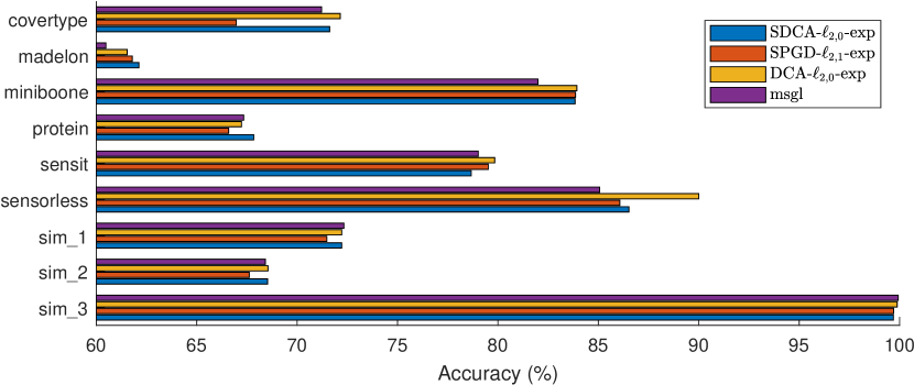
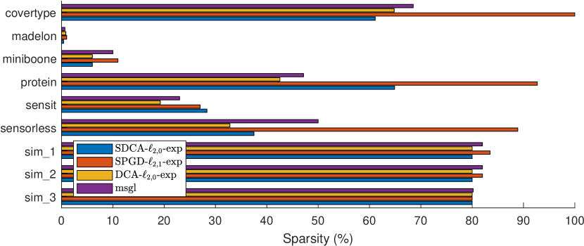
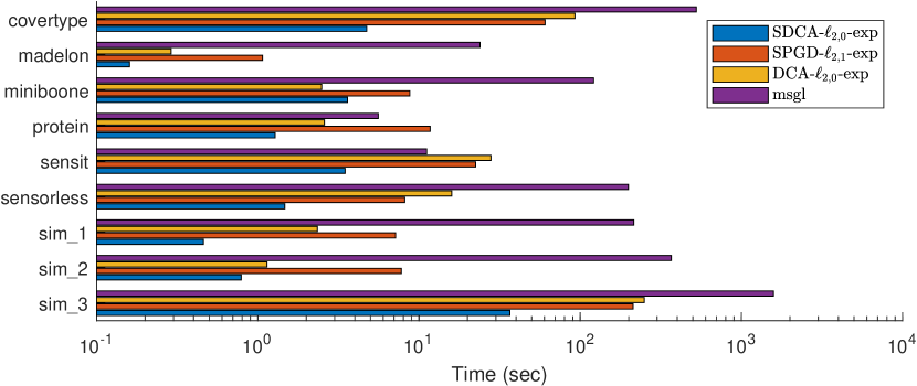
Figure 1: Comparative results between SDCA-$\ell_{2,0}$-exp, DCA-$\ell_{2,0}$-exp, SPGD-$\ell_{2,1}$ and msgl (running time is plotted on a logarithmic scale).

Comparison between SDCA-$\ell_{2,0}$-exp and DCA-$\ell_{2,0}$-exp

In term of classification accuracy, SDCA-$\ell_{2,0}$-exp produces fairly similar result comparing with DCA-$\ell_{2,0}$-exp. DCA-$\ell_{2,0}$-exp is better than SDCA-$\ell_{2,0}$-exp on $4$ datasets (covertype, sensit, sensorless and sim_3) while SDCA-$\ell_{1,0}$-exp gives better results on $2$ datasets (madelon and protein). The two biggest gaps ($3.49\%$ and $1.17\%$) occur on dataset sensorless and sensit respectively.

As for the sparsity of solution, DCA-$\ell_{2,0}$-exp and SDCA-$\ell_{2,0}$-exp provide the same results on $4$ datasets (miniboon, sim_1, sim_2 and sim_3). DCA-$\ell_{2,0}$-exp suppresses more variables than SDCA-$\ell_{2,0}$-exp on $3$ datasets (protein, sensit and sensorless), while SDCA-$\ell_{2,0}$-exp gives better sparsity on covertype and madelon. The gain of DCA-$\ell_{2,0}$-exp on this criterion is quite high, up to $22.3\%$ on dataset protein.

Concerning the running time, SDCA-$\ell_{2,0}$-exp clearly outperforms DCA-$\ell_{2,0}$-exp. Except for miniboone where DCA-$\ell_{2,0}$-exp is $1.11$ second faster, the gain of SDCA-$\ell_{2,0}$-exp is huge. SDCA-$\ell_{2,0}$-exp is up to $19.58$ times faster than DCA-$\ell_{2,0}$-exp (dataset covertype).

Overall, SDCA-$\ell_{2,0}$-exp is able to achieve equivalent classification accuracy with a running time much smaller than DCA-$\ell_{2,0}$-exp.

Comparison between SDCA-$\ell_{2,0}$-exp and msgl.

SDCA-$\ell_{2,0}$-exp provides better classification accuracy on $6$ out of $9$ datasets with a gain up to $1.85\%$. For the $3$ remaining datasets, the gain of msgl in accuracy is smaller than $0.3\%$. As for the sparsity of solution, the two algorithms are comparable. SDCA-$\ell_{2,0}$-exp is by far faster than msgl on all datasets, from $3.2$ times to $470$ time faster.

Comparison between SDCA-$\ell_{2,0}$-exp and SPGD-$\ell_{2,1}$.

In term of classification accuracy, SDCA is better on $6$ datasets with a gain up to $4.65\%$, whereas SPGD only gives better result on sensit. Moreover, the number of selected variables by SPGD-$\ell_{2,1}$ is considerably higher. SPGD-$\ell_{2,1}$ chooses from $2\%$ to $51.39\%$ more variables than SDCA in $6$ over $9$ cases (covertype, miniboone, protein, sensorless, sim_1, and sim_2), and $>27\%$ more in $3$ over $9$ cases (covertype, protein and sensorless). As for the running time, SDCA-$\ell_{2,0}$-exp is up to $15.68$ times faster than SPGD-$\ell_{2,1}$. Overall, SDCA-$\ell_{2,0}$-exp clearly outperforms SPGD-$\ell_{2,1}$ on all three criteria.

In conclusion, as expected, SDCA-$\ell_{2,0}$-exp reduces considerably the running time of DCA-$\ell_{2,0}$-exp while achieving equivalent classification accuracy. Moreover, SDCA-$\ell_{2,0}$-exp outperforms the two related algorithms msgl and SPGD-$\ell_{2,1}$.

4.5 Experiment 2

In this experiment, in order to study the effectiveness of different non-convex regularizations $\ell_{q,0}$, we compare three algorithms SDCA-$\ell_{1,0}$-exp, SDCA-$\ell_{2,0}$-exp and SDCA-$\ell_{\infty,0}$-exp. The results are reported in Table LABEL:tbl.experiment and plotted in Figure 2.

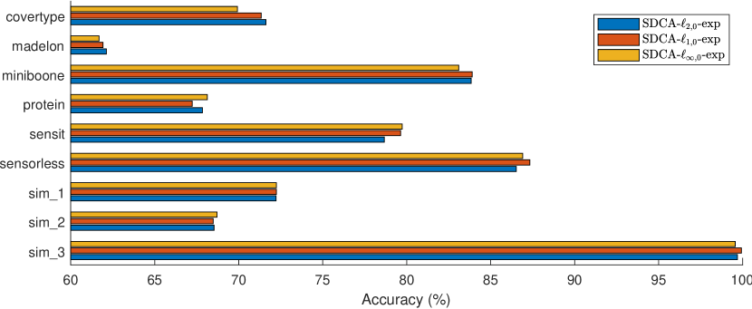
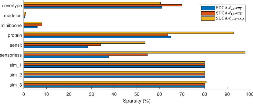
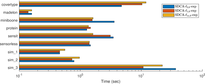
Figure 2: Comparative results between SDCA-$\ell_{1,0}$-exp, SDCA-$\ell_{2,0}$-exp and SDCA-$\ell_{\infty,0}$-exp (running time is plotted on a logarithmic scale).

In term of classification accuracy, SDCA-$\ell_{1,0}$-exp and SDCA-$\ell_{2,0}$-exp are comparable and are slightly better than SDCA-$\ell_{\infty,0}$-exp. SDCA-$\ell_{1,0}$-exp produces similar results with SDCA-$\ell_{2,0}$-exp on $6$ out of $9$ datasets, where the gap is lower than $0.3\%$ in classification accuracy. For protein, sensorless and sensit, SDCA-$\ell_{\infty,0}$-exp provides slightly better classification accuracy than SDCA-$\ell_{1,0}$-exp and SDCA-$\ell_{2,0}$-exp. This is due to the fact that SDCA-$\ell_{\infty,0}$-exp selects much more variables than the two others.

As for the sparsity of solution, SDCA-$\ell_{2,0}$-exp is the best on $8$ out of $9$ datasets (except for protein). SDCA-$\ell_{1,0}$-exp selects moderately more variables than SDCA-$\ell_{2,0}$-exp, from $5.67\%$ to $17.19\%$. In contrast to SDCA-$\ell_{2,0}$-exp, SDCA-$\ell_{\infty,0}$-exp suppresses less variables than SDCA-$\ell_{1,0}$-exp and SDCA-$\ell_{2,0}$-exp on all datasets, except covertype. Especially, on dataset sensorless, SDCA-$\ell_{\infty,0}$-exp selects $60.42\%$ (resp. $43.23\%$) more variables than SDCA-$\ell_{2,0}$-exp (resp. SDCA-$\ell_{1,0}$-exp).

In term of running time, SDCA-$\ell_{1,0}$-exp is the fastest and SDCA-$\ell_{2,0}$-exp is the slowest among the three algorithms. SDCA-$\ell_{1,0}$-exp is up to $3.4$ time faster than SDCA-$\ell_{2,0}$-exp and $2.06$ times faster than SDCA-$\ell_{\infty,0}$-exp.

Overall, SDCA-$\ell_{1,0}$-exp and SDCA-$\ell_{2,0}$-exp provide comparable results and realize a better trade-off between classification and sparsity of solution than SDCA-$\ell_{\infty,0}$-exp.

4.6 Experiment 3

In this experiment, to study the effect of the approximation functions (capped-$\ell_{1}$ and exponential approximation), we compare two algorithms: SDCA-$\ell_{2,0}$-exp and SDCA-$\ell_{2,0}$-cap$\ell_{1}$. It is worth to note that capped-$\ell_{1}$ function is nonsmooth, hence the resulting approximate problem is a nonsmooth (and nonconvex) problem. The results are reported in Figure 3 and Table LABEL:tbl.experiment.

For sensit, madelon, sim_1, sim_2 dataset, both algorithms have similar performance in all three criteria. The differences in terms of accuracy are negligible ($<0.1\%$), while the gaps of sparsity and running time are mostly the same.

For sim_3 and miniboone dataset, both algorithms choose the same number of features. However, SDCA-$\ell_{2,0}$-cap$\ell_{1}$ is faster than SDCA-$\ell_{2,0}$-exp (by $41\%$ and $67\%$ respectively), while SDCA-$\ell_{2,0}$-exp gives better (or similar) result in terms of classification accuracy.

For covertype, sensorless and protein dataset, SDCA-$\ell_{2,0}$-exp provides better results than SDCA-$\ell_{2,0}$-cap$\ell_{1}$. SDCA-$\ell_{2,0}$-exp furnishes results with higher classification accuracy in $2$ out of $3$ cases (covertype and sensorless) while having lower lower sparsity in $2$ out of $3$ cases (protein and sensorless). In terms of running time, SDCA-$\ell_{2,0}$-exp is faster than SDCA-$\ell_{2,0}$-cap$\ell_{1}$ by at least $1.5$ times.

Overall, SDCA-$\ell_{2,0}$-exp clearly shows better results SDCA-$\ell_{2,0}$-cap$\ell_{1}$ in three criteria.

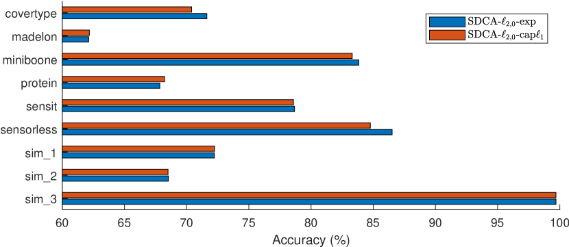
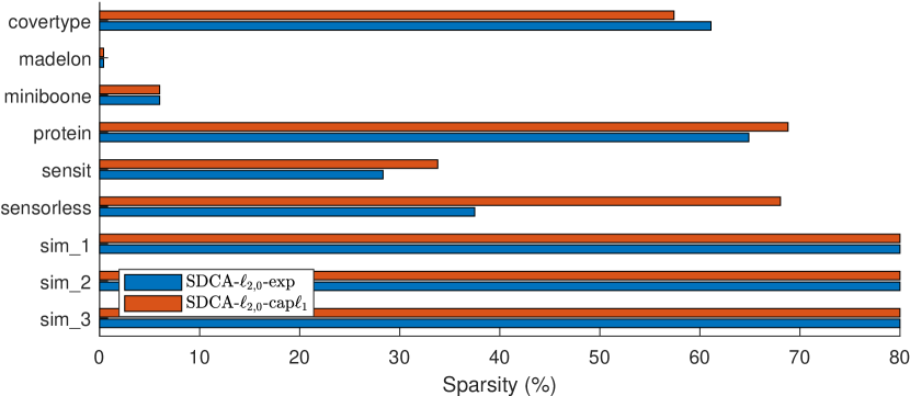
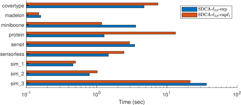
Figure 3: Comparative results between SDCA-$\ell_{2,0}$-exp and SDCA-$\ell_{2,0}$-cap$\ell_{1}$ (running time is plotted on a logarithmic scale).

Table 2: Comparative results on both synthetic and real datasets.
Bold values correspond to best results for each dataset. $n$, $d$ and $Q$ is the number of instances, the number of variables and the number of classes respectively.

Dataset	Algorithm	Accuracy (%)		Time (s)		Sparsity (%)
		Mean	STD	Mean	STD	Mean	STD
covertype	SDCA-$\ell_{2,0}$-exp	71.62	0.05	4.74	0.07	61.11	3.21
$n=581,012$	SDCA-$\ell_{1,0}$-exp	71.34	0.07	10.27	1.25	69.91	1.77
$d=54$	SDCA-$\ell_{\infty,0}$-exp	69.92	0.38	11.93	0.88	60.49	1.51
$Q=7$	SDCA-$\ell_{2,0}$-cap$\ell_{1}$	70.40	0.03	7.47	5.69	57.41	1.85
	SDCA-$\ell_{1,0}$-cap$\ell_{1}$	68.60	0.29	8.98	2.03	25.93	0.00
	SDCA-$\ell_{\infty,0}$-cap$\ell_{1}$	70.16	0.03	14.80	3.63	56.79	3.85
	DCA-$\ell_{2,0}$-exp	72.15	0.08	92.73	0.51	64.81	1.51
	DCA-$\ell_{1,0}$-exp	72.28	0.07	57.93	2.87	73.61	0.93
	DCA-$\ell_{\infty,0}$-exp	69.39	0.10	57.22	5.36	42.13	0.93
	DCA-$\ell_{2,0}$-cap$\ell_{1}$	70.40	0.03	61.15	3.34	57.41	1.85
	DCA-$\ell_{1,0}$-cap$\ell_{1}$	69.41	0.39	37.20	1.23	69.14	1.07
	DCA-$\ell_{\infty,0}$-cap$\ell_{1}$	72.09	0.13	19.99	0.10	49.38	5.35
	SPGD-$\ell_{2,1}$	66.97	0.51	60.59	7.09	100.00	0.00
	msgl	71.22	0.02	525.49	1.10	68.52	0.00
madelon	SDCA-$\ell_{2,0}$-exp	62.12	1.00	0.16	0.02	0.40	0.12
$n=2,600$	SDCA-$\ell_{1,0}$-exp	61.92	0.80	0.14	0.03	0.65	0.10
$d=500$	SDCA-$\ell_{\infty,0}$-exp	61.68	1.05	0.16	0.01	0.70	1.47
$Q=2$	SDCA-$\ell_{2,0}$-cap$\ell_{1}$	62.18	1.35	0.15	0.09	0.40	0.00
	SDCA-$\ell_{1,0}$-cap$\ell_{1}$	61.73	1.26	0.16	0.02	1.53	0.12
	SDCA-$\ell_{\infty,0}$-cap$\ell_{1}$	61.99	1.06	0.16	0.31	10.60	0.20
	DCA-$\ell_{2,0}$-exp	61.54	0.79	0.29	0.27	0.85	0.19
	DCA-$\ell_{1,0}$-exp	61.83	1.12	0.32	0.02	0.55	0.10
	DCA-$\ell_{\infty,0}$-exp	61.88	1.03	2.17	0.01	4.65	0.25
	DCA-$\ell_{2,0}$-cap$\ell_{1}$	61.28	2.23	0.21	0.00	0.93	0.12
	DCA-$\ell_{1,0}$-cap$\ell_{1}$	61.54	1.57	0.41	0.00	1.07	0.31
	DCA-$\ell_{\infty,0}$-cap$\ell_{1}$	60.58	1.07	0.35	0.01	2.73	0.23
	SPGD-$\ell_{2,1}$	61.79	0.80	1.07	0.03	1.00	0.20
	msgl	60.48	2.37	23.92	0.12	0.67	0.00
miniboone	SDCA-$\ell_{2,0}$-exp	83.84	0.08	3.60	0.04	6.00	0.00
$n=130,065$	SDCA-$\ell_{1,0}$-exp	83.90	0.10	1.57	0.06	8.00	0.00
$d=50$	SDCA-$\ell_{\infty,0}$-exp	83.10	0.22	1.62	0.04	8.00	0.00
$Q=2$	SDCA-$\ell_{2,0}$-cap$\ell_{1}$	83.31	0.15	1.18	0.01	6.00	0.00
	SDCA-$\ell_{1,0}$-cap$\ell_{1}$	82.50	0.06	2.96	0.19	8.00	0.00
	SDCA-$\ell_{\infty,0}$-cap$\ell_{1}$	83.77	0.10	4.22	0.28	16.00	4.00
	DCA-$\ell_{2,0}$-exp	83.93	0.12	2.49	0.31	6.00	0.00
	DCA-$\ell_{1,0}$-exp	84.19	0.15	9.42	0.09	8.00	0.00
	DCA-$\ell_{\infty,0}$-exp	81.54	0.12	9.81	3.45	8.00	0.00
	DCA-$\ell_{2,0}$-cap$\ell_{1}$	83.74	0.07	7.04	0.01	6.00	0.00
	DCA-$\ell_{1,0}$-cap$\ell_{1}$	83.11	0.05	7.54	0.00	4.00	0.00
	DCA-$\ell_{\infty,0}$-cap$\ell_{1}$	82.81	0.09	7.14	0.00	15.33	1.15
	SPGD-$\ell_{2,1}$	83.86	0.13	8.77	0.41	11.00	1.15
	msgl	81.99	0.21	121.17	4.30	10.00	0.00
protein	SDCA-$\ell_{2,0}$-exp	67.84	1.11	1.28	0.06	64.89	1.95
$n=24,387$	SDCA-$\ell_{1,0}$-exp	67.23	0.90	1.47	0.02	63.67	2.39
$d=357$	SDCA-$\ell_{\infty,0}$-exp	68.13	0.57	1.36	0.06	92.79	0.86
$Q=3$	SDCA-$\ell_{2,0}$-cap$\ell_{1}$	66.41	1.12	1.13	0.12	22.64	0.47
	SDCA-$\ell_{1,0}$-cap$\ell_{1}$	67.25	1.24	1.33	0.14	65.73	1.09
	SDCA-$\ell_{\infty,0}$-cap$\ell_{1}$	68.19	1.06	1.13	0.10	77.47	0.42
	DCA-$\ell_{2,0}$-exp	67.23	0.75	2.59	0.02	42.56	1.66
	DCA-$\ell_{1,0}$-exp	66.19	0.96	3.77	0.41	33.36	1.87
	DCA-$\ell_{\infty,0}$-exp	66.93	0.75	13.53	2.12	54.21	0.61
	DCA-$\ell_{2,0}$-cap$\ell_{1}$	67.04	0.72	3.35	0.00	50.47	1.27
	DCA-$\ell_{1,0}$-cap$\ell_{1}$	67.89	0.60	3.43	0.00	79.68	0.58
	DCA-$\ell_{\infty,0}$-cap$\ell_{1}$	66.90	0.84	3.66	1.04	58.43	1.46
	SPGD-$\ell_{2,1}$	66.59	1.82	11.73	2.80	92.70	2.50
	msgl	67.34	0.48	5.59	0.36	47.15	1.32
sensit	SDCA-$\ell_{2,0}$-exp	78.67	0.11	3.48	0.21	28.33	8.50
$n=98,528$	SDCA-$\ell_{1,0}$-exp	79.64	0.22	3.11	0.96	34.00	17.35
$d=100$	SDCA-$\ell_{\infty,0}$-exp	79.73	0.28	1.61	0.07	53.67	6.81
$Q=3$	SDCA-$\ell_{2,0}$-cap$\ell_{1}$	78.59	0.08	2.94	0.17	33.80	5.31
	SDCA-$\ell_{1,0}$-cap$\ell_{1}$	79.71	0.23	2.94	2.12	100.00	0.00
	SDCA-$\ell_{\infty,0}$-cap$\ell_{1}$	78.83	0.24	2.91	0.20	35.00	2.74
	DCA-$\ell_{2,0}$-exp	79.84	0.11	27.97	0.80	19.25	0.50
	DCA-$\ell_{1,0}$-exp	79.65	0.21	18.31	4.90	17.50	0.58
	DCA-$\ell_{\infty,0}$-exp	79.16	0.17	42.91	5.24	91.50	2.38
	DCA-$\ell_{2,0}$-cap$\ell_{1}$	78.92	0.15	26.36	2.22	56.67	1.53
	DCA-$\ell_{1,0}$-cap$\ell_{1}$	78.91	0.38	27.05	2.80	57.33	0.58
	DCA-$\ell_{\infty,0}$-cap$\ell_{1}$	79.20	0.17	35.78	2.69	91.67	7.23
	SPGD-$\ell_{2,1}$	79.52	0.27	22.44	2.41	27.00	1.00
	msgl	79.02	0.13	11.16	0.53	23.00	0.00
sensorless	SDCA-$\ell_{2,0}$-exp	86.52	0.78	1.47	0.16	37.50	5.10
$n=58,509$	SDCA-$\ell_{1,0}$-exp	87.33	0.27	1.40	0.09	54.69	10.67
$d=48$	SDCA-$\ell_{\infty,0}$-exp	86.91	0.19	1.41	0.38	97.92	2.08
$Q=11$	SDCA-$\ell_{2,0}$-cap$\ell_{1}$	84.77	0.08	2.45	0.13	68.06	1.20
	SDCA-$\ell_{1,0}$-cap$\ell_{1}$	82.89	0.30	2.69	0.62	72.92	2.08
	SDCA-$\ell_{\infty,0}$-cap$\ell_{1}$	87.12	0.72	1.36	0.09	25.69	1.20
	DCA-$\ell_{2,0}$-exp	90.00	0.31	15.96	0.65	32.81	1.04
	DCA-$\ell_{1,0}$-exp	89.11	0.18	16.28	0.97	31.25	0.00
	DCA-$\ell_{\infty,0}$-exp	90.76	0.14	18.99	0.81	100.00	0.00
	DCA-$\ell_{2,0}$-cap$\ell_{1}$	89.60	1.15	24.75	1.39	53.47	1.20
	DCA-$\ell_{1,0}$-cap$\ell_{1}$	88.87	1.04	16.28	0.44	47.92	0.80
	DCA-$\ell_{\infty,0}$-cap$\ell_{1}$	81.06	3.9	14.99	3.22	41.67	0.70
	SPGD-$\ell_{2,1}$	86.07	1.39	8.16	1.05	88.89	2.41
	msgl	85.06	0.31	199.00	41.75	50.00	0.00
sim_1	SDCA-$\ell_{2,0}$-exp	72.22	0.46	0.46	0.02	80.00	0.00
$n=100,000$	SDCA-$\ell_{1,0}$-exp	72.24	0.43	0.46	0.03	80.00	0.00
$d=50$	SDCA-$\ell_{\infty,0}$-exp	72.24	0.47	0.56	0.06	80.00	0.00
$Q=4$	SDCA-$\ell_{2,0}$-cap$\ell_{1}$	72.24	0.52	0.50	0.04	80.00	0.00
	SDCA-$\ell_{1,0}$-cap$\ell_{1}$	72.24	0.58	0.42	0.06	80.00	0.00
	SDCA-$\ell_{\infty,0}$-cap$\ell_{1}$	72.21	0.58	0.51	0.07	80.00	0.00
	DCA-$\ell_{2,0}$-exp	72.22	0.40	2.34	0.05	80.00	0.00
	DCA-$\ell_{1,0}$-exp	72.25	0.38	0.26	0.01	80.00	0.00
	DCA-$\ell_{\infty,0}$-exp	72.22	0.40	9.79	0.10	80.00	0.00
	DCA-$\ell_{2,0}$-cap$\ell_{1}$	72.25	0.52	0.32	0.00	80.00	0.00
	DCA-$\ell_{1,0}$-cap$\ell_{1}$	72.24	0.52	0.30	0.00	80.00	0.00
	DCA-$\ell_{\infty,0}$-cap$\ell_{1}$	72.24	0.51	3.00	0.00	80.00	0.00
	SPGD-$\ell_{2,1}$	71.48	0.81	7.16	0.91	83.50	2.52
	msgl	72.33	0.18	214.83	25.40	82.00	0.00
sim_2	SDCA-$\ell_{2,0}$-exp	68.53	0.29	0.79	0.00	80.00	0.00
$n=150,000$	SDCA-$\ell_{1,0}$-exp	68.48	0.34	0.73	0.16	80.00	0.00
$d=50$	SDCA-$\ell_{\infty,0}$-exp	68.71	0.23	0.97	0.12	80.00	0.00
$Q=3$	SDCA-$\ell_{2,0}$-cap$\ell_{1}$	68.50	0.29	1.02	0.14	80.00	0.00
	SDCA-$\ell_{1,0}$-cap$\ell_{1}$	67.42	0.40	0.71	0.23	80.00	0.00
	SDCA-$\ell_{\infty,0}$-cap$\ell_{1}$	68.38	0.28	1.40	0.18	80.00	0.00
	DCA-$\ell_{2,0}$-exp	68.55	0.22	1.14	0.26	80.00	0.00
	DCA-$\ell_{1,0}$-exp	68.31	0.23	13.51	1.93	80.00	0.00
	DCA-$\ell_{\infty,0}$-exp	68.71	0.18	2.75	2.80	80.00	0.00
	DCA-$\ell_{2,0}$-cap$\ell_{1}$	67.70	0.31	4.29	0.03	80.00	0.00
	DCA-$\ell_{1,0}$-cap$\ell_{1}$	68.43	0.24	0.93	0.16	80.00	0.00
	DCA-$\ell_{\infty,0}$-cap$\ell_{1}$	67.49	0.35	0.69	0.10	80.00	0.00
	SPGD-$\ell_{2,1}$	67.62	0.48	7.77	0.28	82.00	0.00
	msgl	68.42	0.03	367.29	53.52	82.00	0.00
sim_3	SDCA-$\ell_{2,0}$-exp	99.69	0.04	36.61	1.48	80.00	0.00
$n=250,000$	SDCA-$\ell_{1,0}$-exp	99.93	0.01	10.74	0.42	80.00	0.00
$d=500$	SDCA-$\ell_{\infty,0}$-exp	99.56	0.07	22.11	3.43	80.73	0.64
$Q=4$	SDCA-$\ell_{2,0}$-cap$\ell_{1}$	99.69	0.01	21.45	0.93	80.00	0.00
	SDCA-$\ell_{1,0}$-cap$\ell_{1}$	99.00	0.01	23.10	0.12	80.00	0.00
	SDCA-$\ell_{\infty,0}$-cap$\ell_{1}$	99.67	0.01	21.05	1.06	80.00	0.00
	DCA-$\ell_{2,0}$-exp	99.88	0.02	249.74	10.73	80.00	0.00
	DCA-$\ell_{1,0}$-exp	99.88	0.02	202.67	33.27	80.00	0.00
	DCA-$\ell_{\infty,0}$-exp	97.74	2.05	431.13	26.47	80.00	0.00
	DCA-$\ell_{2,0}$-cap$\ell_{1}$	99.92	0.01	178.89	7.83	80.00	0.00
	DCA-$\ell_{1,0}$-cap$\ell_{1}$	99.87	0.01	270.69	17.64	80.00	0.00
	DCA-$\ell_{\infty,0}$-cap$\ell_{1}$	99.85	0.03	24.40	4.29	80.40	0.40
	SPGD-$\ell_{2,1}$	99.70	0.12	212.71	21.79	80.00	0.00
	msgl	99.93	0.01	1581.44	14.76	80.20	0.00

5 Conclusion

We have proposed two novel DCA based algorithms, stochastic DCA and inexact stochastic DCA for minimizing a large sum of DC functions, with the aim of reducing the computation cost of DCA in large-scale setting. The sum structure of the objective function $F$ permits us to work separately on the component functions $F_{i}$. The stochastic DCA is then proposed to tackle problems with huge numbers of $F_{i}$ while the inexact stochastic DCA aims to address large-scale setting and big data. We have carefully studied the convergence properties of the proposed algorithms. It turns out that the convergence to a critical point of both stochastic DCA and inexact stochastic DCA is guaranteed with probability $1$. Furthermore, we have developed DCA and SDCA to group variables selection in multi-class logistic regression, an important problem in machine learning. By using a suitable DC decomposition of the objective function we have designed a DCA scheme in which all computations are explicit and inexpensive. Consequently SDCA is very inexpensive. Numerical results showed that, as expected, SDCA-$\ell_{2,0}$-exp reduces considerably the running time of DCA-$\ell_{2,0}$-exp while achieving equivalent classification accuracy. Moreover, SDCA-$\ell_{2,0}$-exp outperforms the two related algorithms msgl and SPGD-$\ell_{2,1}$. We are convinced that SDCA is an efficient variant of DCA, especially for large-scale setting.

Continuing this research direction, in future works we will develop novel versions of DCA based algorithms (e.g. online/stochastic/approximate/like DCA) for other problems in order to accelerate the convergence of DCA and to deal with large-scale setting and big data.

Appendix A Proof of Theorem 2

To prove Theorem 2, we will use the following lemma.

Lemma 1.

Let $f:\mathbb{R}^{d}\to\mathbb{R}\cap\{+\infty\}$ be a $\rho$-convex function. For any $\epsilon\geq 0$ and any $v\in\partial_{\epsilon}f(x)$ with $x\in$ dom $f$, we have

$$2\epsilon+f(y)\geq f(x)+\langle v,y-x\rangle+\frac{\rho}{4}\|y-x\|^{2},\ \forall y\in\mathbb{R}^{d}.$$

Proof.

Since $v\in\partial_{\epsilon}f(x)$, we have

$$\epsilon+f(z)\geq f(x)+\langle v,z-x\rangle,\ \forall z\in\mathbb{R}^{d}.$$

Replacing $z$ with $x+t(y-x)$ in this inequality gives that

$$\epsilon+f(x+t(y-x))\geq f(x)+t\langle v,y-x\rangle,\ \forall y\in\mathbb{R}^{d}.$$

It follows from the $\rho$-convexity of $f$ that for $y\in\mathbb{R}^{d}$ and $t\in(0,1)$,

$$tf(y)+(1-t)f(x)\geq f(x+t(y-x))+\frac{\rho t(1-t)}{2}\|y-x\|^{2}.$$

Summing the two above inequalities gives us

$$\epsilon+tf(y)\geq tf(x)+t\langle v,y-x\rangle+\frac{\rho t(1-t)}{2}\|y-x\|^{2}.$$

Thus, the conclusion follows from this inequality with $t=1/2$. ∎

Proof.

(of Theorem 2) a) Let $x^{0}_{i}$ be the copies of $x^{0}$. We set $x^{l+1}_{i}=x^{l+1}$ for all $i\in s_{l+1}$ and $x^{l+1}_{j}=x^{l}_{j}$ for $j\not\in s_{l+1}$. Set $\epsilon^{0}_{i}=\epsilon^{0}$ and $\epsilon^{l+1}_{i}=\epsilon^{l+1}$ if $i\in s_{l+1}$, $\epsilon^{l}_{i}$ otherwise. We then have $v^{l}_{i}\in\partial_{\epsilon^{l}_{i}}h_{i}(x_{i}^{l})$ for $i=1,...,n$. Let $T_{i}^{l}$ be the function given by

$$T_{i}^{l}(x)=g_{i}(x)-h_{i}(x_{i}^{l})-\left\langle x-x_{i}^{l},v^{l}_{i}\right\rangle+2\epsilon^{l}_{i}.$$

It follows from $v^{l}_{i}\in\partial_{\epsilon^{l}_{i}}h_{i}(x_{i}^{l})$ that

$$\epsilon^{l}_{i}+h_{i}(x)\geq h_{i}(x_{i}^{l})+\left\langle x-x_{i}^{l},v^{l}_{i}\right\rangle.$$

This implies $T_{i}^{l}(x)\geq F_{i}(x)+\epsilon^{l}_{i}\geq F_{i}(x)$ for all $l\geq 0$, $i=1,...,n$. We also observe that $x^{l+1}$ is an $\epsilon^{l}$-solution of the following convex problem

$$\min_{x}T^{l}(x):=\frac{1}{n}\sum_{i=1}^{n}T_{i}^{l}(x)$$ (30)

Therefore

$$T^{l}(x^{l+1})\leq T^{l}(x^{l})+\epsilon^{l} =T^{l-1}(x^{l})+\frac{1}{n}\sum_{i\in s_{l}}[T_{i}^{l}(x^{l})-T_{i}^{l-1}(x^{l})]+\epsilon^{l}$$ (31)

$$=T^{l-1}(x^{l})+\frac{1}{n}\sum_{i\in s_{l}}[F_{i}(x^{l})+2\epsilon^{l}-T_{i}^{l-1}(x^{l})]+\epsilon^{l},$$

where the second equality follows from $T_{i}^{l}(x^{l})=F_{i}(x^{l})+2\epsilon^{l}$ for all $i\in s_{l}$. Let $\mathcal{F}_{l}$ denote the $\sigma$-algebra generated by the entire history of ISDCA up to the iteration $l$, i.e., $\mathcal{F}_{0}=\sigma(x^{0},\epsilon^{0})$ and $\mathcal{F}_{l}=\sigma(x^{0},...,x^{l},\epsilon^{0},...,\epsilon^{l},s_{0},...,s_{l-1})$ for all $l\geq 1$. By taking the expectation of the inequality (31) conditioned on $\mathcal{F}_{l}$, we have

$$\mathbb{E}\left[T^{l}(x^{l+1})|\mathcal{F}_{l}\right]\leq T^{l-1}(x^{l})-\frac{b}{n}\left[T^{l-1}(x^{l})-F(x^{l})\right]+\left(\frac{2b}{n}+1\right)\epsilon^{l}.$$

Since $\sum_{l=0}^{\infty}\epsilon^{l}_{i}<+\infty$ with probability $1$, by applying the supermartingale convergence theorem [Neveu, 1975, Bertsekas et al., 2003] to the nonnegative sequences $\{T^{l-1}(x^{l})-\alpha^{*}\},\{\frac{b}{n}[T^{l-1}(x^{l})-F(x^{l})]\}$ and $\{(\frac{2b}{n}+1)\epsilon^{l}\}$, we conclude that the sequence $\{T^{l-1}(x^{l},y^{l})-\alpha^{*}\}$ converges to $T^{*}-\alpha^{*}$ and

$$\sum_{l=1}^{\infty}\left[T^{l-1}(x^{l})-F(x^{l})\right]<\infty,$$ (32)

with probability $1$. Therefore $\{F(x^{l})\}$ converges almost surely to $T^{*}$.

b) By $v_{i}^{l-1}\in\partial_{\epsilon^{l-1}_{i}}h_{i}(x_{i}^{l-1})$ and Lemma 1, we have

$$2\epsilon^{l-1}_{i}+h_{i}(x)\geq h_{i}(x_{i}^{l-1})+\langle x-x_{i}^{l-1},v_{i}^{l-1}\rangle+\frac{\rho(h_{i})}{4}\|x-x_{i}^{l-1}\|^{2},\ \forall x\in\mathbb{R}^{d}.$$

This implies

$$F_{i}(x)\leq T_{i}^{l-1}(x)-\frac{\rho(h_{i})}{4}\|x-x_{i}^{l-1}\|^{2}.$$ (33)

From (31) and (33) with $x=x^{l}$, we have

$$T^{l}(x^{l+1})\leq T^{l-1}(x^{l})-\frac{1}{n}\sum_{i\in s_{l}}\frac{\rho(h_{i})}{4}\|x-x_{i}^{l-1}\|^{2}+\left(\frac{2b}{n}+1\right)\epsilon^{l}.$$ (34)

Taking the expectation of the inequality (34) conditioned on $\mathcal{F}_{l}$, we obtain

$$\mathbb{E}\left[T^{l}(x^{l+1})|\mathcal{F}_{l}\right]\leq T^{l-1}(x^{l})-\frac{b}{4n^{2}}\sum_{i=1}^{n}\rho(h_{i})\|x^{l}-x_{i}^{l-1}\|^{2}+\left(\frac{2b}{n}+1\right)\epsilon^{l}.$$

Combining this and $\rho=\min_{i=1,...,n}\rho(h_{i})>0$ gives us

$$\mathbb{E}\left[T^{l}(x^{l+1})|\mathcal{F}_{l}\right]\leq T^{l-1}(x^{l})-\frac{b\rho}{4n^{2}}\sum_{i=1}^{n}\|x^{l}-x_{i}^{l-1}\|^{2}+\left(\frac{2b}{n}+1\right)\epsilon^{l}.$$

Applying the supermartingale convergence theorem to the nonnegative sequences $\{T^{l-1}(x^{l})-\alpha^{*}\},\{\frac{b}{4\rho n^{2}}\sum_{i=1}^{n}\|x^{l}-x_{i}^{l-1}\|^{2}\}$ and $\{(\frac{2b}{n}+1)\epsilon^{l}\}$, we get

$$\sum_{l=1}^{\infty}\sum_{i=1}^{n}\|x^{l}-x_{i}^{l-1}\|^{2}<\infty,$$

with probability $1$. In particular, for $i=1,...,n$, we have

$$\sum_{l=1}^{\infty}\|x^{l}-x_{i}^{l-1}\|^{2}<\infty,$$ (35)

and hence $\lim_{l\rightarrow\infty}\|x^{l}-x_{i}^{l-1}\|=0$ almost surely.

c) Assume that there exists a sub-sequence $\{x^{l_{k}}\}$ of $\{x^{l}\}$ such that $x^{l_{k}}\rightarrow x^{*}$ almost surely. From (35), we have $\|x^{l_{k}+1}-x_{i}^{l_{k}}\|\rightarrow 0$ almost surely. Without loss of generality, we can suppose that the sub-sequence $v_{i}^{l_{k}}\rightarrow v^{*}_{i}$ almost surely. From the proof of (a), we have

$$\frac{1}{n}\sum_{i=1}^{n}\epsilon^{l}_{i}\leq T^{l}(x^{l+1})-F(x^{l+1}).$$

From this and (32) it follows that $\epsilon^{l}_{i}$ converges to $0$ as $l\to+\infty$ with probability $1$. Since $v_{i}^{l_{k}}\in\partial_{\epsilon_{i}^{l_{k}}}h_{i}(x_{i}^{l_{k}})$, $\epsilon^{l_{k}}_{i}\to 0$ with probability $1$, and by the closed property of the $\epsilon$-subdifferential mapping $\partial_{\epsilon_{i}^{l_{k}}}h_{i}$, we have $v^{*}_{i}\in\partial h_{i}(x^{*})$. Since $x^{l_{k}+1}$ is a $\epsilon^{l_{k}}$-solution of the problem $\min_{x}T^{l_{k}}(x)$, we obtain

$$T^{l_{k}}(x^{l_{k}+1})\leq T^{l_{k}}(x)+\epsilon^{l_{k}}.$$ (36)

Taking $k\rightarrow\infty$ gives us

$$\limsup_{l_{k}\to+\infty}G(x^{l_{k}+1})\leq G(x)-\langle x-x^{*},v^{*}\rangle,\ \forall x\in\mathbb{R}^{d},$$

with probability $1$, where $v^{*}=\frac{1}{n}\sum_{i=1}^{n}v^{*}_{i}\in\partial H(x^{*})$ almost surely. It follows from this with $x=x^{*}$ that

$$\limsup_{l_{k}\to+\infty}G(x^{l_{k}+1})\leq G(x^{*}),$$

almost surely. Combining this with the lower semi-continuity of $G$ gives us that

$$\lim_{l_{k}\to+\infty}G(x^{l_{k}+1})=G(x^{*}),$$

almost surely. Thus, we have

$$G(x^{*})\leq G(x)-\langle x-x^{*},v^{*}\rangle,\ \forall x\in\mathbb{R}^{d},$$

almost surely. This implies

$$v^{*}\in\partial G(x^{*}),$$ (37)

with probability one. Therefore,

$$v^{*}\in\partial G(x^{*})\cap\partial H(x^{*}),$$ (38)

with probability $1$. This implies that $x^{*}$ is a critical point of $F$ with probability $1$ and the proof is then complete. ∎

References

- Allen-Zhu & Yuan [2016] Allen-Zhu, Z., & Yuan, Y. (2016). Improved SVRG for non-strongly-convex or sum-of-non-convex objectives. In Proceedings of the 33rd International Conference on International Conference on Machine Learning - Volume 48 ICML’16 (pp. 1080–1089).
- Bagley et al. [2001] Bagley, S. C., White, H., & Golomb, B. A. (2001). Logistic regression in the medical literature: Standards for use and reporting, with particular attention to one medical domain. Journal of Clinical Epidemiology, 54, 979–985.
- Bertsekas et al. [2003] Bertsekas, D., Nedic, A., & Ozdaglar, A. (2003). Convex analysis and optimization. Athena Scientific.
- Bertsekas [2010] Bertsekas, D. P. (2010). Incremental Gradient, Subgradient, and Proximal Methods for Convex Optimization: A Survey. Technical Report Laboratory for Information and Decision Systems, MIT, Cambridge, MA.
- Bertsekas [2011] Bertsekas, D. P. (2011). Incremental proximal methods for large scale convex optimization. Mathematical Programming, 129, 163–195.
- Bottou [1998] Bottou, L. (1998). On-line learning and stochastic approximations. In D. Saad (Ed.), On-line Learning in Neural Networks (pp. 9–42). New York, NY, USA: Cambridge University Press.
- Boyd et al. [1987] Boyd, C. R., Tolson, M. A., & Copes, W. S. (1987). Evaluating trauma care: The TRISS method. Trauma Score and the Injury Severity Score. The Journal of Trauma, 27, 370–378.
- Bradley & Mangasarian [1998] Bradley, P. S., & Mangasarian, O. L. (1998). Feature selection via concave minimization and support vector machines. In Machine Learning Proceedings of the Fifteenth International Conference (ICML ’98) (pp. 82–90). Morgan Kaufmann.
- Cox [1958] Cox, D. (1958). The regression analysis of binary sequences (with discussion). J Roy Stat Soc B, 20, 215–242.
- Defazio et al. [2014a] Defazio, A., Bach, F., & Lacoste-Julien, S. (2014a). Saga: A fast incremental gradient method with support for non-strongly convex composite objectives. In Proceedings of Advances in Neural Information Processing Systems.
- Defazio et al. [2014b] Defazio, A., Caetano, T., & Domke, J. (2014b). Finito: A faster, permutable incremental gradient method for big data problems. In Proceedings of the International Conference on Machine Learning.
- Genkin et al. [2007] Genkin, A., Lewis, D. D., & Madigan, D. (2007). Large-scale Bayesian logistic regression for text categorization. Technometrics, 49, 291–304.
- Healy & Schruben [1991] Healy, K., & Schruben, L. W. (1991). Retrospective simulation response optimization. In 1991 Winter Simulation Conference Proceedings. (pp. 901–906).
- Johnson & Zhang [2013] Johnson, R., & Zhang, T. (2013). Accelerating stochastic gradient descent using predictive variance reduction. In Advances in Neural Information Processing Systems 26 (pp. 315–323). Curran Associates Inc.
- Kim et al. [2008] Kim, J., Kim, Y., & Kim, Y. (2008). A Gradient-Based Optimization Algorithm for LASSO. Journal of Computational and Graphical Statistics, 17, 994–1009.
- King & Zeng [2001] King, G., & Zeng, L. (2001). Logistic Regression in Rare Events Data. Political Analysis, 9, 137–163.
- Le Thi et al. [2008] Le Thi, H. A., Le, H. M., Nguyen, V. V., & Pham Dinh, T. (2008). A DC programming approach for feature selection in support vector machines learning. Advances in Data Analysis and Classification, 2, 259–278.
- Le Thi et al. [2017] Le Thi, H. A., Le, H. M., Phan, D. N., & Tran, B. (2017). Stochastic DCA for the Large-sum of Non-convex Functions Problem and its Application to Group Variable Selection in Classification. In Proceedings of the 34th International Conference on Machine Learning (pp. 3394–3403). volume 70.
- Le Thi & Pham Dinh [2005] Le Thi, H. A., & Pham Dinh, T. (2005). The DC (difference of convex functions) programming and DCA revisited with DC models of real world nonconvex optimization problems. Annals of Operations Research, 133, 23–46.
- Le Thi & Pham Dinh [2018] Le Thi, H. A., & Pham Dinh, T. (2018). DC programming and DCA: thirty years of developments. Mathematical Programming, (pp. 1–64).
- Le Thi et al. [2015] Le Thi, H. A., Pham Dinh, T., Le, H. M., & Vo, X. T. (2015). DC approximation approaches for sparse optimization. Eur. J. Oper. Res., 244, 26–46.
- Le Thi & Phan [2016] Le Thi, H. A., & Phan, D. N. (2016). DC Programming and DCA for Sparse Optimal Scoring Problem. Neurocomput., 186, 170–181.
- Le Thi et al. [2019] Le Thi, H. A., Phan, D. N., & Pham, D. T. (2019). DCA based approaches for bi-level variable selection and application for estimating multiple sparse covariance matrices. Revised version Neurocomputing, .
- Le Thi [Home Page] Le Thi (Home Page), H. A. (2005). DC Programming and DCA - Website of Le Thi Hoai An. http://www.lita.univ-lorraine.fr/~lethi/index.php/en/research/dc-programming-and-dca.html.
- LeCun et al. [1998] LeCun, Y., Bottou, L., Orr, G. B., & Müller, K. R. (1998). Efficient backprop. In Neural Networks: Tricks of the Trade (pp. 9–50). Berlin, Heidelberg: Springer Berlin Heidelberg.
- Liao & Chin [2007] Liao, J. G., & Chin, K.-V. (2007). Logistic regression for disease classification using microarray data: Model selection in a large p and small n case. Bioinformatics, 23, 1945–1951.
- Mairal [2015] Mairal, J. (2015). Incremental majorization-minimization optimization with application to large-scale machine learning. SIAM Journal on Optimization, 25, 829–855.
- Neveu [1975] Neveu, J. (1975). Discrete-Parameter Martingales volume 10 of North-Holland Mathematical Library. Elsevier.
- Parikh & Boyd [2014] Parikh, N., & Boyd, S. (2014). Proximal algorithms. Found. Trends Optim., 1, 127–239.
- Pham Dinh & Le Thi [1997] Pham Dinh, T., & Le Thi, H. A. (1997). Convex analysis approach to dc programming: Theory, algorithms and applications. Acta Mathematica Vietnamica, 22, 289–355.
- Pham Dinh & Le Thi [1998] Pham Dinh, T., & Le Thi, H. A. (1998). A D. C. Optimization Algorithm for Solving the Trust-Region Subproblem. SIAM Journal of Optimization, 8, 476–505.
- Pham Dinh & Le Thi [2014] Pham Dinh, T., & Le Thi, H. A. (2014). Recent advances in DC programming and DCA. Transactions on Computational Collective Intelligence, 8342, 1–37.
- Pham Dinh & Souad [1986] Pham Dinh, T., & Souad, E. B. (1986). Algorithms for Solving a Class of Nonconvex Optimization Problems. Methods of Subgradients. In J. B. Hiriart-Urruty (Ed.), North-Holland Mathematics Studies (pp. 249–271). North-Holland volume 129 of Fermat Days 85: Mathematics for Optimization.
- Phan et al. [2017] Phan, D. N., Le Thi, H. A., & Pham Dinh, T. (2017). Sparse covariance matrix estimation by DCA-Based Algorithms. Neural Computation, 29, 3040–3077.
- Phan & Thi [2019] Phan, D. N., & Thi, H. A. L. (2019). Group variable selection via regularization and application to optimal scoring. Neural Networks, .
- Reddi et al. [2016] Reddi, S. J., Sra, S., Poczos, B., & Smola, A. J. (2016). Proximal stochastic methods for Nonsmooth Nonconvex Finite-Sum Optimization. In Advances in Neural Information Processing Systems (pp. 1145–1153).
- Robbins & Monro [1951] Robbins, H., & Monro, S. (1951). A stochastic approximation method. The Annals of Mathematical Statistics, 22, 400–407.
- Schmidt et al. [2017] Schmidt, M., Le Roux, N., & Bach, F. (2017). Minimizing finite sums with the stochastic average gradient. Mathematical Programming, 162, 83–112.
- Shalev-Schwartz & Zhang [2013] Shalev-Schwartz, S., & Zhang, T. (2013). Stochastic dual coordinate ascent methods for regularized loss minimization. Journal of Machine Learning Research, 14, 567–599.
- Subasi & Erçelebi [2005] Subasi, A., & Erçelebi, E. (2005). Classification of EEG signals using neural network and logistic regression. Comput. Methods Programs Biomed., 78, 87–99.
- Vincent & Hansen [2014] Vincent, M., & Hansen, N. R. (2014). Sparse group lasso and high dimensional multinomial classification. Comput. Stat. Data Anal., 71, 771–786.
- Witten & Tibshirani [2011] Witten, D. M., & Tibshirani, R. (2011). Penalized classification using Fisher’s linear discriminant. Journal of the Royal Statistical Society: Series B, 73, 753–772.