The Lidov–Kozai Oscillation and Hugo von Zeipel^∗

Abstract

The circular restricted three-body problem, particularly its doubly averaged version, has been very well studied in celestial mechanics. Despite its simplicity, circular restricted three-body systems are suited for modeling the motion of various objects in the solar system, extrasolar planetary systems, and in many other dynamical systems that show up in astronomical studies. In this context, the so-called Lidov–Kozai oscillation is well known and applied to various objects. This makes the orbital inclination and eccentricity of the perturbed body in the circular restricted three-body system oscillate with a large amplitude under certain conditions. It also causes a libration of the perturbed body’s argument of pericenter around stationary points. It is widely accepted that the theoretical framework of this phenomenon was established independently in the early 1960s by a Soviet Union dynamicist (Michail L’vovich Lidov) and by a Japanese celestial mechanist (Yoshihide Kozai). Since then, the theory has been extensively studied and developed. A large variety of studies has stemmed from the original works by Lidov and Kozai, now having the prefix of “Lidov–Kozai” or “Kozai–Lidov.” However, from a survey of past literature published in late nineteenth to early twentieth century, we have confirmed that there already existed a pioneering work using a similar analysis of this subject established in that period. This was accomplished by a Swedish astronomer, Edvard Hugo von Zeipel. In this monograph, we first outline the basic framework of the circular restricted three-body problem including typical examples where the Lidov–Kozai oscillation occurs. Then, we introduce what was discussed and learned along this line of studies from the early to mid-twentieth century by summarizing the major works of Lidov, Kozai, and relevant authors. Finally, we make a summary of von Zeipel’s work, and show that his achievements in the early twentieth century already comprehended most of the fundamental and necessary formulations that the Lidov–Kozai oscillation requires. By comparing the works of Lidov, Kozai, and von Zeipel, we assert that the prefix “von Zeipel–Lidov–Kozai” should be used for designating this theoretical framework, and not just Lidov–Kozai or Kozai–Lidov. This justifiably shows due respect and appropriately commemorates these three major pioneers who made significant contributions to the progress of modern celestial mechanics.

1 Introduction

Solar system dynamics has a large diversity of aspects. We know that it encompasses many complicated and unsolved problems. But we also know that it is filled with rich and interesting characteristics of nonlinear dynamical systems. In spite of the general complexity of solar system dynamics, it is also true that the orbital motion of many of the solar system objects can be fairly well approximated by perturbed Keplerian motion, and the magnitude of perturbation is usually moderate or small. This is due to the existence of the very strong gravity from a massive central body, the Sun. The major source of the gravitational perturbation against the two-body Keplerian motion is the planets.

Having the feature of this kind as a background, the restricted three-body problem (hereafter referred to as R3BP), a variant of the general three-body problem, often becomes a good proxy in solar system dynamics. In R3BP, the mass of one of the three bodies is assumed to be so small that it does not affect the motion of the other two bodies at all. Therefore, R3BP is particularly appropriate when we deal with the orbital motion of small objects (such as asteroids, comets, transneptunian objects, natural and artificial satellites) under the perturbation resulting from the major planets.

When the massive two bodies compose a circular binary in R3BP, the problem is particularly called the circular restricted three-body problem (hereafter referred to as CR3BP). In spite of its very simple setting, we can still use CR3BP as a good proxy in many cases in solar system dynamics. This is mainly due to the moderate to very small eccentricity of the major planets in the current solar system. Thanks to its simple configuration and small degrees of freedom, CR3BP has played an important role in the development of analytic perturbation theories, and it is still applied to many subjects in modern celestial mechanics. As we will see later in greater detail, we can reduce the degrees of freedom of CR3BP into unity through the double averaging procedure of the disturbing function (a function that represents the perturbing force). This makes the system integrable, and it enables us to obtain a global picture of the perturbed (third) body’s motion, even when the perturbed body’s eccentricity or inclination is substantially large.

Based on the integrable characteristics of the doubly averaged CR3BP, the theory of the so-called Lidov–Kozai oscillation has emerged. This is the major subject of this monograph. Chronologically speaking, a Soviet Union dynamicist, Michail L’vovich Lidov, found in 1961 that, when dealing with the motion of Earth-orbiting satellites under the perturbation from other objects as CR3BP, the satellites’ argument of pericenter can librate around $\pm\frac{\pi}{2}$ when their initial orbital inclination is larger than a certain value. The eccentricity and inclination of the perturbed body exhibit a synchronized periodic oscillation under this circumstance. Almost at the same time, a Japanese celestial mechanist, Yoshihide Kozai, dealt with the motion of asteroids orbiting inside Jupiter’s orbit as CR3BP, and found in 1962 that, an asteroid’s argument of perihelion can librate around $\pm\frac{\pi}{2}$ when its initial orbital inclination is larger than a certain value. The two works by Lidov and Kozai turned out to be theoretically equivalent, and the dynamical phenomenon is now collectively referred to as the Lidov–Kozai oscillation. Note that although we basically use the term “oscillation” in the present monograph, many other different terms have been used for the same phenomenon in the literature, such as “mechanism,” “resonance,” “cycle,” “effect,” and so on. See Section 6.2.5 for more detail about the choice of terms.

After the series of publications by Lidov and Kozai in the 1960s, this dynamical phenomenon became better known, and found applications in the fields of astronomy, planetary science, and astronautics. Their theories have been applied not only to the long-term motion of Earth-orbiting satellites that Lidov considered or the secular asteroidal dynamics that Kozai pursued in their era, but also to the motion of other solar system objects such as irregular satellites, various comets, near-Earth asteroids, and transneptunian objects. In particular, the discovery of extrasolar planets and their orbital configurations of a great variety resulted in a recognition that the Lidov–Kozai oscillation has played a significant role in the evolution of these dynamical systems. The development of the Lidov–Kozai oscillation still goes on, incorporating higher-order perturbations and more subtle and complicated physical effects such as general relativity and the combination with mean motion resonances. Recent application of the Lidov–Kozai oscillation even extends to stellar dynamics, and its theory is employed for explaining various problems such as formation of some kind of binaries and triple star systems, merger mechanism of binary black holes, modeling the galactic tide, and so forth.

Part of the purpose of this monograph is to outline how the Lidov–Kozai oscillation works, who developed the theory, and in what way. We will briefly mention what kind of applications have been considered since the era of Lidov and Kozai up to the present. However, this is not our predominant aim. In this monograph, we wish to draw attention to the fact that a pioneering work in this line of study had been carried out long before the era of Lidov and Kozai. More specifically, most of the basic ingredients that Lidov or Kozai presented for the doubly averaged CR3BP, including the necessary condition of argument of pericenter’s libration, had been already recognized, quantitatively investigated, and published on journals by 1910. This was accomplished by a Swedish astronomer, Hugo von Zeipel.

As far as our investigation shows, the work by von Zeipel in 1910 has been ignored and buried in oblivion for a long time, regardless of its substantial significance and excellent foresight in solar system dynamics. The major purpose of this monograph is to validate the correctness of von Zeipel’s work, and to redirect the attention of the relevant communities to this pioneering study that was established and published at the beginning of the twentieth century.

The complete table of contents for this monograph is in its online version. Supplementary Information 1 also gives the same table with specific page number information. For readers who do not particularly specialize in the dynamical aspects of astronomy or planetary science, Section 2 summarizes what CR3BP is and what kind of phenomena the Lidov–Kozai oscillation causes, employing simple numerical demonstrations. In the following sections, we will review the achievements of Lidov and Kozai by summarizing two classic papers: Kozai (1962) in Section 3, and Lidov (1961) in Section 4. We will also browse through an earlier work on CR3BP in the former Soviet Union (Moiseev, 1945a, b) in Section 4. Finally in Section 5, we summarize von Zeipel’s work published in 1910. This is the kernel of this monograph. Section 6 presents discussions, but it also includes additional matters of even earlier works by von Zeipel. Readers that are already familiar with the work by Kozai or Lidov may want to skip Sections 2, 3, 4, and proceed straight to Section 5. Yet, readers should note that in Sections 5 and 6 we often refer to facts, equations, and figures described in Sections 2, 3, 4. Also, note that Sections 3, 4, and 5 are not placed in chronological order. We place them in the order that these works gained recognition. Although Lidov (1961) was published earlier than Kozai (1962), Kozai’s work began gaining attention earlier than Lidov’s work. Whereas von Zeipel’s work was published much earlier than the others, it has not been recognized to this day.

In this monograph we basically use the conventional notation for the Keplerian orbital elements: $a$ for semimajor axis, $e$ for eccentricity, and $I$ or $i$ for inclination. As for argument of pericenter and longitude of ascending node, we prefer the notation used for the Delaunay elements ($g$ and $h$, respectively), rather than the conventional ones ($\omega$ and $\Omega$). But sometimes we use $\omega$ and $\Omega$, particularly in Section 4, because Lidov uses $\omega$ and $\Omega$, not $g$ and $h$. We use the standard notations $L,G,H$ for the actions of the Delaunay elements. We use $l$ for mean anomaly, and $n$ for mean motion.

Note that there are several notations in this monograph that may cause confusion among readers. Examples are:

• In von Zeipel’s work, therefore in our Section 5, he uses the symbol $\Theta$ for denoting one of the Delaunay elements $(\Theta=G\cos i)$, instead of the conventional notation $H$. He uses the symbol $H$ for denoting another, different angle in his work.

• In Kozai’s work, therefore in our Section 3, $\Theta$ is used for denoting an important, but totally different quantity.

• ${\cal H}$, a calligraphic style of $H$, is sometimes used for denoting Hamiltonian in this monograph (e.g. Eq. (32)).

• ${\cal G}$, a calligraphic style of $G$, denotes the gravitational constant in this monograph (e.g. Eqs. (9) and (10)).

For avoiding potential clutter and confusion, we try to give definitions of the variables used in this monograph as clearly as possible whenever they first show up, or whenever they are used in different meanings than before.

As for the equation numbering, we try to follow the ways used in the original literature as much as possible. More specifically, when we cite equations that show up in one of the following literature, we give them the following designations in this monograph: “K” for Kozai (1962), “L” for Lidov (1961), “Mb” for Moiseev (1945b), or “Z” for von Zeipel (1910) $+$ equation number in the original publication $+$ “-” $+$ sequential equation number in this monograph. Here are some examples of our equation numbering:

• Eq. (28) in Kozai (1962) $\to$ (K28-83)

• Eq. (2.16) in Moiseev (1945b) $\to$ (Mb2.16-125)

• Eq. (7) in Lidov (1961) $\to$ (L07-135)

• Eq. (103) in von Zeipel (1910) $\to$ (Z103-340)

Other equations in this monograph that do not have a leading K, L, M, or Z in their equation number are either those which do not appear in the above literature, or those which appear without equation number in the above literature. Also, sometimes we cite page numbers, section and subsection numbers, and chapter numbers of the above literature in the same manner such as “p. K592” (designating p. 592 of Kozai (1962)) or “Section Z1” (designating Section 1 of von Zeipel (1910)).

In this monograph we cite many publications written in non-English language such as French, German, Swedish, Russian, and Japanese. We basically reproduced their bibliographic information using their original language in the References section (p. 6.6–References). However, use of the Cyrillic alphabets and the Japanese characters is prohibited in the main body of the monograph due to a technical limitation about font in the LaTeX typesetting process by the publisher. Because of this, for listing the literature that uses the Cyrillic and Japanese characters in the Reference section, we translated their bibliographic information into English. But we believe that the bibliographic information of the non-English literature written in their original language is quite valuable for the readers of this monograph. Another point to note is that, some hyperlinks to the Uniform Resource Locators (URLs) embedded in the References section do not properly function, although the URLs themselves are correct. This is due to another technical limitation in this monograph’s LaTeX typesetting process. For these two reasons we have created a more complete, alternative bibliography for this monograph using the Cyrillic and Japanese characters with fully functional hyperlinks. We put it in Supplementary Information 2 which is free from the technical limitations.

This monograph minimizes the use of URLs in the text mainly due to the technical limitation of embedded hyperlinks mentioned above. We also wanted to avoid clutter by having many complicated URLs that often become sources of distractions. Instead, in Supplementary Information 3 we made a list of the URLs of relevant websites that we mention in this monograph, such as orbital databases of the small solar system bodies. On the other hand, most of the literature listed in the References section of this monograph are accompanied by explicit URLs that are hyperlinked to each of their online resources.

Now that the Lidov–Kozai oscillation has gained a great popularity, a number of good review papers and textbooks that deal with the fundamentals and applications of this phenomenon in substantial depth have been published (e.g. Morbidelli, 2002; Merritt, 2013; Davies et al., 2014; Naoz, 2016). A doctoral dissertation (Antognini, 2016) that entirely devotes itself to the study of this phenomenon is also publicly available. Readers who have a deeper interest in the Lidov–Kozai oscillation, and those who want to seek further applications of the theory, can consult these works. In addition, a textbook that totally dedicates itself to the Lidov–Kozai oscillation has been recently published (Shevchenko, 2017). As expected, we found that the contents of some part of this monograph (particularly Sections 3 and 4) overlap with Shevchenko (2017). We included these two sections in this monograph to state our own view of what Kozai and Lidov achieved, as well as what they did not, in the light of von Zeipel’s publications. In other words, the major purpose of this monograph is to sketch and highlight the similarities and differences between the works of Kozai, Lidov, and von Zeipel. Hence we need our Sections 3 and 4.

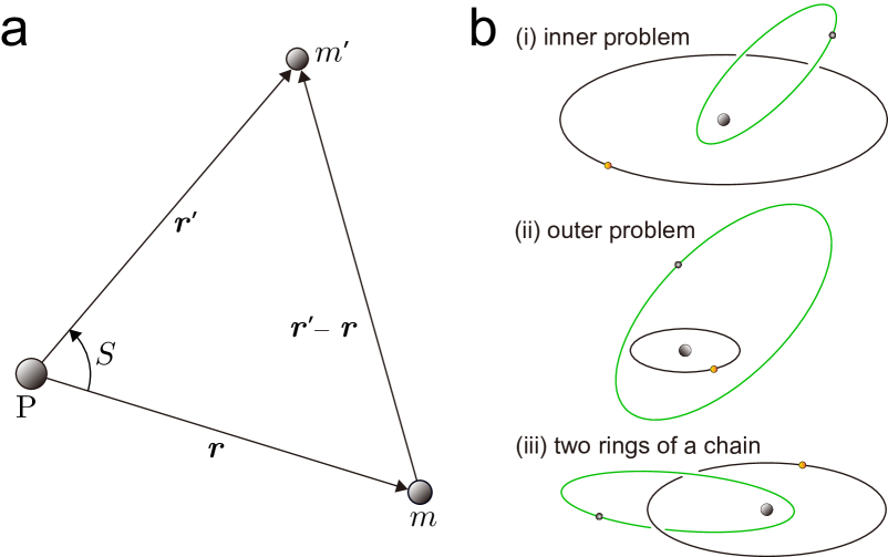
Figure 1: Schematic illustrations of the three-body system that we consider in this monograph. a: Relative geometric configuration of a three-body system centered at the primary mass (P). See Section 2.2 for the meanings of the symbols ($\bm{r}$, $\bm{r^{\prime}}$, $m$, $m^{\prime}$, $S$). b: Three typical patterns of the restricted three-body problem. (i) The inner problem where the perturbed body’s orbit (the green ellipse) lies inside the orbit of the perturbing body (the black ellipse). (ii) The outer problem where the perturbed body’s orbit (the green ellipse) lies outside the orbit of the perturbing body (the black ellipse). (iii) When two bodies behave like the rings of a chain. Note that the phrase “like the rings of a chain” is adopted from von Zeipel (1910, “comme les anneaux d’une chaîne” on p. 378, and “comme deux anneaux d’une chaîne” on p. 413).

2 Preliminaries: What We Consider

This section presents a simple illustration of the system that we deal with in this monograph—the circular restricted three-body problem. Our intention is to facilitate readers’ understanding of what we discuss in later sections.

The two-body problem is integrable, and has an exact analytic solution—the Keplerian motion described by various conic sections. However, just by adding one more mass to the system, the system ceases to have such a general solution. The three-body problem is not integrable, and we have no exact analytic solution except in very few special cases. This fact was already known at the end of the nineteenth century. Bruns (1887) proved the algebraic non-integrability of the general three-body problem. Poincaré (1890) soon gave a proof of the non-existence of an integral in the restricted three-body system: The analytic non-integrability of the restricted three-body problem was proven. However, we should recall that it is this very non-integrability of the three-body problem that has resulted in a large number of interesting and important aspects of nonlinear dynamics published in vast amount of the past literature, such as collisional singularities, periodic orbits, resonances, and chaos. It is also the reason why the three-body problem has attracted many scientists from a variety of fields over a long time, yielding a great deal of achievement. For the modern progress of the three-body problem in general, readers can consult many literature (e.g. Valtonen and Karttunen, 2006; Valtonen et al., 2016; Musielak and Quarles, 2014). A short summary of the development of studies of the three-body problem during the late nineteenth and twentieth centuries is available in Ito and Tanikawa (2007, their Section 3).

The dynamics of a three-body system is sometimes highly chaotic. However, it can also be very regular and nearly integrable, depending on the mass ratio and the initial orbit configurations between the three bodies. Fortunately in the current solar system, a nearly-integrable hierarchical three-body system often becomes a good proxy of dynamics. A hierarchical three-body system comprises a massive central primary (the mass $m_{0}$) accompanied by a less massive secondary (the mass $m_{1}<m_{0}$), as well as an even less massive tertiary (the mass $m_{2}<m_{1}$). The tertiary mass orbits inside or outside the $(m_{0},m_{1})$ binary. Unless the orbit of the secondary around the primary and that of the tertiary around the primary get too close or intersect each other, the two binaries, $(m_{0},m_{1})$ and $(m_{0},m_{2})$, usually behave in the nearly integrable manner (i.e. close to the Keplerian motion). In that case, we can principally obtain their orbital solution through perturbation methods. The $(m_{0},m_{1})$ binary would make a pure Keplerian motion if $m_{2}\ll m_{1}$, not being disturbed by $m_{2}$ at all, while the motion of $m_{2}$ is affected by the $(m_{0},m_{1})$ binary. This is the restricted three-body problem (R3BP). In particular, when the orbit of $m_{1}$ in the $(m_{0},m_{1})$ binary is circular, the system results in the circular restricted three-body problem (CR3BP). Note that the restricted three-body problem is often dealt with in a rotating coordinate system where massive bodies ($m_{0}$ and $m_{1}$) always stay on the $x$-axis (e.g. Quarles et al., 2012). However, we do not adopt the rotating coordinate system in this monograph. Readers can consult Szebehely (1967) for more general and detailed characteristics of the restricted three-body problems, particularly those considered in a rotating frame.

2.1 Relative motion

Let us briefly summarize how the basic equations of motion that describe the dynamics of a three-body system are derived in a standard way. For making our descriptions in this monograph consistent with conventional literature, we use the relative coordinates centered on $m_{0}$, instead of the Jacobi coordinates (e.g. Plummer, 1960; Wisdom and Holman, 1991) or other canonical coordinates. The discussion in this subsection follows Brouwer and Clemence (1961, Chapters X and XII), Danby (1992, Subsections 9.4 and 11.12), Murray and Dermott (1999, Subsection 6.2), and Merritt (2013, Subsection 4.8) on the whole.

We write the position vectors of the three bodies with masses $m_{0}$, $m_{1}$, $m_{2}$ with respect to a fixed origin in the inertial reference frame as $\bm{\xi}_{0},\bm{\xi}_{1},\bm{\xi}_{2}$. In addition, we denote the relative position vector of the secondary mass $m_{1}$ with respect to the primary mass $m_{0}$ as

$$\bm{r}_{1}\equiv\bm{\xi}_{1}-\bm{\xi}_{0}=\left(\begin{array}[]{c}x_{1}\\ y_{1}\\ z_{1}\end{array}\right).$$ (1)

Similarly, the relative position vector of the tertiary mass $m_{2}$ with respect to the primary mass $m_{0}$ is denoted as

$$\bm{r}_{2}\equiv\bm{\xi}_{2}-\bm{\xi}_{0}=\left(\begin{array}[]{c}x_{2}\\ y_{2}\\ z_{2}\end{array}\right).$$ (2)

The distance between the secondary and tertiary masses is

$$\left|\bm{r}_{2}-\bm{r}_{1}\right|=\sqrt{\left(x_{2}-x_{1}\right)^{2}+\left(y_{2}-y_{1}\right)^{2}+\left(z_{2}-z_{1}\right)^{2}}.$$ (3)

Using $\bm{\xi}_{0},\bm{\xi}_{1},\bm{\xi}_{2}$ and $\bm{r}_{1},\bm{r}_{2}$, we can determine and reduce the equations of motion of the three bodies in the inertial reference frame as follows:

$$m_{0}\frac{d^{2}\bm{\xi}_{0}}{dt{}^{2}} ={\cal G}m_{0}m_{1}\frac{\bm{r}_{1}}{r_{1}^{3}}+{\cal G}m_{0}m_{2}\frac{\bm{r}_{2}}{r_{2}^{3}},$$ (4)

$$m_{1}\frac{d^{2}\bm{\xi}_{1}}{dt{}^{2}} =-{\cal G}m_{1}m_{0}\frac{\bm{r}_{1}}{r_{1}^{3}}+{\cal G}m_{1}m_{2}\frac{\bm{r}_{2}-\bm{r}_{1}}{\left|\bm{r}_{2}-\bm{r}_{1}\right|^{3}},$$ (5)

$$m_{2}\frac{d^{2}\bm{\xi}_{2}}{dt{}^{2}} =-{\cal G}m_{2}m_{0}\frac{\bm{r}_{2}}{r_{2}^{3}}+{\cal G}m_{2}m_{1}\frac{\bm{r}_{1}-\bm{r}_{2}}{\left|\bm{r}_{1}-\bm{r}_{2}\right|^{3}},$$ (6)

where ${\cal G}$ is the gravitational constant, $t$ denotes time, $r_{1}\equiv\left|\bm{r}_{1}\right|$, and $r_{2}\equiv\left|\bm{r}_{2}\right|$.

Now, let us determine the equations of motion of the secondary mass expressed on the relative reference frame centered on the primary mass. From Eq. (1) we have

$$\frac{d^{2}\bm{\xi}_{1}}{dt{}^{2}}=\frac{d^{2}\bm{r}_{1}}{dt{}^{2}}+\frac{d^{2}\bm{\xi}_{0}}{dt{}^{2}}.$$ (7)

Similarly, the equations of motion of the tertiary mass expressed on the relative reference frame centered on the primary mass are, from Eq. (2)

$$\frac{d^{2}\bm{\xi}_{2}}{dt{}^{2}}=\frac{d^{2}\bm{r}_{2}}{dt{}^{2}}+\frac{d^{2}\bm{\xi}_{0}}{dt{}^{2}}.$$ (8)

We eliminate $\frac{d^{2}\bm{\xi}_{0}}{dt{}^{2}}$ from the right-hand sides of Eqs. (7) and (8) using the quantity in the right-hand side of Eq. (4): substitution of $\frac{d^{2}\bm{\xi}_{0}}{dt{}^{2}}={\cal G}m_{1}\frac{\bm{r}_{1}}{r_{1}^{3}}+{\cal G}m_{2}\frac{\bm{r}_{2}}{r_{2}^{3}}$. Then, as for the mass $m_{1}$, we substitute $\frac{d^{2}\bm{\xi}_{1}}{dt{}^{2}}$ of Eq. (7) into Eq. (5). As for the mass $m_{2}$, we substitute $\frac{d^{2}\bm{\xi}_{2}}{dt{}^{2}}$ of Eq. (8) into Eq. (6). Eventually we obtain their relative equations of motion as:

$$\frac{d^{2}\bm{r}_{1}}{dt{}^{2}}+{\cal G}\left(m_{0}+m_{1}\right)\frac{\bm{r}_{1}}{r_{1}^{3}} ={\cal G}m_{2}\left(\frac{\bm{r}_{2}-\bm{r}_{1}}{\left|\bm{r}_{2}-\bm{r}_{1}\right|^{3}}-\frac{\bm{r}_{2}}{r_{2}^{3}}\right),$$ (9)

$$\frac{d^{2}\bm{r}_{2}}{dt{}^{2}}+{\cal G}\left(m_{0}+m_{2}\right)\frac{\bm{r}_{2}}{r_{2}^{3}} ={\cal G}m_{1}\left(\frac{\bm{r}_{1}-\bm{r}_{2}}{\left|\bm{r}_{1}-\bm{r}_{2}\right|^{3}}-\frac{\bm{r}_{1}}{r_{1}^{3}}\right).$$ (10)

Now it is straightforward to confirm that the terms in the right-hand side of Eqs. (9) and (10) can be rewritten as gradients of certain scalar functions. Let us write them as $R_{1}$ and $R_{2}$. Their actual forms are as follows:

$$\frac{d^{2}\bm{r}_{1}}{dt{}^{2}}+{\cal G}\left(m_{0}+m_{1}\right)\frac{\bm{r}_{1}}{r_{1}^{3}} =\nabla R_{1},$$ (11)

$$\frac{d^{2}\bm{r}_{2}}{dt{}^{2}}+{\cal G}\left(m_{0}+m_{2}\right)\frac{\bm{r}_{2}}{r_{2}^{3}} =\nabla R_{2},$$ (12)

where

$$R_{1} \equiv\frac{{\cal G}m_{2}}{\left|\bm{r}_{2}-\bm{r}_{1}\right|}-{\cal G}m_{2}\frac{\bm{r}_{1}\cdot\bm{r}_{2}}{r_{2}^{3}},$$ (13)

$$R_{2} \equiv\frac{{\cal G}m_{1}}{\left|\bm{r}_{1}-\bm{r}_{2}\right|}-{\cal G}m_{1}\frac{\bm{r}_{2}\cdot\bm{r}_{1}}{r_{1}^{3}}.$$ (14)

$R_{1}$ in Eq. (13) and $R_{2}$ in Eq. (14) are called the disturbing function for the mass $m_{1}$ and the mass $m_{2}$, respectively. They represent the gravitational interaction between $m_{1}$ and $m_{2}$. The major gravitational force exerted from the primary mass $m_{0}$ is expressed as the second term in the left-hand side of Eq. (11) or Eq. (12). If we ignore the disturbing function $R_{1}$ from the right-hand side of Eq. (11), the motion of the mass $m_{1}$ would be the pure Keplerian motion around $m_{0}$. Similarly if we ignore the disturbing function $R_{2}$ from the right-hand side of Eq. (12), the motion of the mass $m_{2}$ would be the pure Keplerian motion around $m_{0}$.

The first terms of the disturbing functions (13) and (14) are called the direct part, representing the major component of the mutual perturbation between $m_{1}$ and $m_{2}$. The second terms are called the indirect part, which originate from the choice of the coordinate system. The indirect part would not exist if we took the origin of the coordinate system to be the center of mass (e.g. Murray and Dermott, 1999; Ellis and Murray, 2000). Also, the indirect part vanishes or becomes constant when we carry out an averaging of the system. Thus they do not contribute to secular dynamics of the system unless non-negligible mean motion resonances are at work and the employment of averaging procedure is prohibited.

2.2 Disturbing function

Let us restate the equation of motion of the secondary (11) and that of the tertiary (12) in a more convenient form. Following the descriptions in conventional textbooks, we change the notation as follows: $m_{0}\to M$, $m_{1}\to m$, $m_{2}\to m^{\prime}$, $\bm{r}_{1}\to\bm{r}$, $\bm{r}_{2}\to\bm{r^{\prime}}$, $R_{1}\to R$, and $R_{2}\to\widetilde{R}$. We define the angle between $\bm{r}$ and $\bm{r}^{\prime}$ as $S$. We show the geometric configuration of the system under this notation in a schematic figure (Fig. 1a).

The rewritten equations of motion of the mass $m$ (former $m_{1}$) become from Eq. (11)

$$\frac{d^{2}\bm{r}}{dt{}^{2}}+{\cal G}\left(M+m\right)\frac{\bm{r}}{r^{3}}=\nabla R,$$ (15)

and the rewritten equations of motion of the mass $m^{\prime}$ (former $m_{2}$) become from Eq. (12)

$$\frac{d^{2}\bm{r}^{\prime}}{dt{}^{2}}+{\cal G}\left(M+m^{\prime}\right)\frac{\bm{r}^{\prime}}{{r^{\prime}}^{3}}=\nabla\widetilde{R}.$$ (16)

The disturbing function for Eq. (15) is, from Eq. (13)

$$R=\frac{{\cal G}m^{\prime}}{\Delta}-{\cal G}m^{\prime}\frac{\bm{r}\cdot\bm{r}^{\prime}}{{r^{\prime}}^{3}},$$ (17)

and the disturbing function for Eq. (16) is, from Eq. (14)

$$\widetilde{R}=\frac{{\cal G}m}{\Delta}-{\cal G}m\frac{\bm{r}^{\prime}\cdot\bm{r}}{r^{3}},$$ (18)

with the conventional notation for the mutual distance

$$\Delta\equiv\left|\bm{r}^{\prime}-\bm{r}\right|=\left|\bm{r}-\bm{r}^{\prime}\right|.$$ (19)

Note that $\widetilde{R}$ in Eqs. (16) and (18) is often denoted as $R^{\prime}$ in the conventional literature.

In this monograph we will consider only the direct part of the disturbing function (the first terms in the right-hand sides of Eqs. (17) and (18)). The indirect part of the disturbing function (the second terms in the right-hand sides of Eqs. (17) and (18)) does not play any significant roles in the doubly averaged system described below.

We can expand the disturbing function $R$ or $\widetilde{R}$ in an infinite series of orbital elements. There are several different ways to do this. Here we consider one of the most straightforward ways: the expansion using the Legendre polynomials. Applying the cosine formula to the triangle $m$–P–$m^{\prime}$ with the angle $S$ in Fig. 1a, we get

$$\left|\bm{r}^{\prime}-\bm{r}\right|^{2}=r^{2}+{r^{\prime}}^{2}-2rr^{\prime}\cos S.$$ (20)

Using Eq. (20), we can expand $\Delta$ in Eq. (19) through the Legendre polynomials $P_{j}$. When $r<r^{\prime}$, it becomes

$$\frac{1}{\Delta} =\frac{1}{r^{\prime}}\left(1-2\frac{r}{r^{\prime}}\cos S+\left(\frac{r}{r^{\prime}}\right)^{2}\right)^{-\frac{1}{2}}$$ (21)

$$=\frac{1}{r^{\prime}}\sum_{j=0}^{\infty}\left(\frac{r}{r^{\prime}}\right)^{j}P_{j}(\cos S).$$

On the other hand when $r>r^{\prime}$, it becomes

$$\frac{1}{\Delta} =\frac{1}{r}\left(1-2\frac{r^{\prime}}{r}\cos S+\left(\frac{r^{\prime}}{r}\right)^{2}\right)^{-\frac{1}{2}}$$ (22)

$$=\frac{1}{r}\sum_{j=0}^{\infty}\left(\frac{r^{\prime}}{r}\right)^{j}P_{j}(\cos S).$$

Let us regard the mass $m$ as the perturbed body, and the mass $m^{\prime}$ as the perturbing body. The orbital condition $r<r^{\prime}$ required for the expression of $\Delta$ in Eq. (21) indicates that the perturbed body’s orbit always stays inside that of the perturbing body (see Fig. 1b(i)). We call it the inner problem. In this case, the term with $j=0$ in the expansion of $\Delta$ in Eq. (21) does not depend on $r$ at all. As we saw in the equations of relative motion (15), what matters is not $R$ itself, but its derivative $\nabla R$. The $j=0$ terms in Eq. (21) obviously disappears through this differentiation, Henceforth we can ignore the $j=0$ terms in Eq. (21) from our discussion. In addition, we have the relationship

$$\bm{r}\cdot\bm{r^{\prime}}=rr^{\prime}\cos S=rr^{\prime}P_{1}(\cos S),$$ (23)

and we can apply it to the indirect part of the disturbing function (the second term in the right-hand side of Eq. (17)). Then, we find that the indirect part of the disturbing function cancels out the term of $j=1$ in Eq. (21), and both of them disappear in the expression of $R$. Therefore for the disturbing function of the inner problem, we need to consider only the $j\geq 2$ terms in the expansions of $\Delta$ in Eq. (21) as

$$\frac{1}{\Delta}=\frac{1}{r^{\prime}}\sum_{j=2}^{\infty}\left(\frac{r}{r^{\prime}}\right)^{j}P_{j}(\cos S).$$ (24)

When the other orbital condition $(r>r^{\prime})$ takes place with the expression of $\Delta$ in Eq. (22), the perturbed body’s orbit always stays outside that of the perturbing body (see Fig. 1b(ii)). We call it the outer problem. In this case, unlike the inner case, the exact cancellation of the indirect part of the disturbing function does not happen (see Murray and Dermott, 1999, Eq. (6.23) on p. 229). Specifically writing down all the relevant terms, $R$ for the outer problem in Eq. (17) becomes (omitting the coefficient ${\cal G}m$)

$$\frac{1}{r}\sum_{j=2}^{\infty}\left(\frac{r^{\prime}}{r}\right)^{j}P_{j}(\cos S)+\frac{1}{r}+\frac{r^{\prime}}{r^{2}}\cos S-\frac{r}{{r^{\prime}}^{2}}\cos S.$$ (25)

The second term $\left(\frac{1}{r}\right)$ in Eq. (25) comes from the $j=0$ term in Eq. (22), but it becomes a constant after we average the disturbing function over the fast-oscillating variables (consult Section 2.3 of this monograph for the details of the averaging procedure of the disturbing function). Therefore we do not need to consider this term in the discussion. The third term comes from the $j=1$ term in Eq. (22), and the fourth term originates from the indirect part in Eq. (17). Both of these disappear after the averaging procedure. As a consequence, it turns out that what we need to consider is only the $j\geq 2$ terms in the expansion of $\frac{1}{\Delta}$ in Eq. (22) for the averaged outer problem.

When the orbit of the perturbed body and that of the perturbing body cross each other and behave like the rings of a chain (i.e. when $r$ can be either smaller or larger than $r^{\prime}$. See Fig. 1b(iii)), the expansion of the disturbing function using the Legendre polynomials in Eq. (21) or Eq. (22) does not work out anymore. It is because $\frac{r}{r^{\prime}}$ $\bigl{(}\mbox{or }\frac{r^{\prime}}{r}\bigr{)}$ can exceed unity, and the infinite series in Eq. (21) or Eq. (22) does not converge. We will briefly mention this case later again (Section 5.5 or Section 5.8 of this monograph).

Carrying out literal expansions of the disturbing function is a formidable task in general. But it is relatively simpler in CR3BP, particularly in its doubly averaged version. We will see some examples later in this monograph. In CR3BP, the length of the position vector of the perturber $(r^{\prime})$ with respect to the primary mass has a constant value that is equivalent to its semimajor axis, $a^{\prime}$. And when $r^{\prime}=a^{\prime}$, we do not need to consider the odd terms $(j=3,5,7,\cdots)$ in the expansion of Eqs. (21) and (22) at all, because they all vanish after the averaging procedure. Therefore the disturbing function for the inner CR3BP ($r<r^{\prime}$) that we consider turns out as, from Eqs. (17) and (21):

$$R=\frac{{\cal G}m^{\prime}}{a^{\prime}}\sum_{n=1}^{\infty}\left(\frac{r}{a^{\prime}}\right)^{2n}P_{2n}(\cos S).$$ (26)

On the other hand for the outer CR3BP ($r>r^{\prime}$), $R$ becomes from Eqs. (17) and (22) as

$$R=\frac{{\cal G}m^{\prime}}{r}\sum_{n=1}^{\infty}\left(\frac{a^{\prime}}{r}\right)^{2n}P_{2n}(\cos S).$$ (27)

Although we do not show it here, it is clear that we can carry out the expansion of $\widetilde{R}$ in Eq. (18) in a similar manner whenever necessary.

Let us note in passing that, in the inner problem, the direct part of the disturbing function $\frac{{\cal G}m^{\prime}}{\Delta}$ can be derived in a different, more general way. Return temporarily to a general three-body system with three masses: the primary $m_{0}$, secondary $m_{1}$, and tertiary $m_{2}$. Now let us use the Jacobi coordinates where we measure $m_{1}$’s position vector $\tilde{\bm{r}}_{1}$ from $m_{0}$, and measure $m_{2}$’s position vector $\tilde{\bm{r}}_{2}$ from the barycenter of $m_{0}$ and $m_{1}$ (here we assume $\tilde{r}_{1}<\tilde{r}_{2}$ for the inner problem). We define an angle $S_{12}$ as the angle between the vectors $\tilde{\bm{r}}_{1}$ and $\tilde{\bm{r}}_{2}$. In general, $S_{12}$ is different from $S$ in Fig. 1a, and the origins of $\bm{r}_{1}$ and $\bm{r}_{2}$ are different from each other. Then, the equations of motion of the secondary mass $m_{1}$ and the tertiary mass $m_{2}$ become (e.g. Smart, 1953; Brouwer and Clemence, 1961; Jefferys and Moser, 1966)

$$\tilde{m}_{1}\frac{d^{2}\tilde{\bm{r}}_{1}}{dt^{2}}=\frac{\partial F}{\partial\tilde{\bm{r}}_{1}},\quad\tilde{m}_{2}\frac{d^{2}\tilde{\bm{r}}_{2}}{dt^{2}}=\frac{\partial F}{\partial\tilde{\bm{r}}_{2}},$$ (28)

where

$$\tilde{m}_{1}=\frac{m_{0}m_{1}}{m_{0}+m_{1}},\quad\tilde{m}_{2}=\frac{\left(m_{0}+m_{1}\right)m_{2}}{m_{0}+m_{1}+m_{2}},$$ (29)

are the reduced masses used in the Jacobi coordinates (e.g. Wisdom and Holman, 1991; Saha and Tremaine, 1994). Here $F$ is the common force function

$$F ={\cal G}\left[\frac{m_{0}m_{1}}{\tilde{r}_{1}}+\frac{(m_{0}+m_{1})m_{2}}{\tilde{r}_{2}}\right.$$ (30)

$$\quad\quad\quad+\left.\frac{1}{\tilde{r}_{2}}\sum_{j=2}^{\infty}M_{j}\left(\frac{\tilde{r}_{1}}{\tilde{r}_{2}}\right)^{j}P_{j}(\cos S_{12})\right],$$

and $M_{j}$ is the mass factor

$$M_{j}=\frac{m_{0}m_{1}m_{2}\left(m_{0}^{j-1}-\left(-m_{1}\right)^{j-1}\right)}{\left(m_{0}+m_{1}\right)^{j}}.$$ (31)

Using the force function $F$, we can construct a Hamiltonian that governs the dynamics of this system. Assuming $a_{1}$ and $a_{2}$ to be the semimajor axes of the orbits of the secondary and tertiary masses, the Hamiltonian ${\cal H}$ becomes (e.g. Harrington, 1968; Krymolowski and Mazeh, 1999; Beust and Dutrey, 2006; Carvalho et al., 2013):

$${\cal H} =\frac{{\cal G}m_{0}m_{1}}{2a_{1}}+\frac{{\cal G}(m_{0}+m_{1})m_{2}}{2a_{2}}$$ (32)

$$\quad\quad\quad+\frac{\cal G}{\tilde{r}_{2}}\sum_{j=2}^{\infty}M_{j}\left(\frac{\tilde{r}_{1}}{\tilde{r}_{2}}\right)^{j}P_{j}(\cos S_{12}).$$

The first term of ${\cal H}$ in Eq. (32) is responsible for the Keplerian motion of the secondary mass, and the second term is responsible for that of the tertiary mass. The third term of ${\cal H}$ represents the mutual interaction of the secondary and the tertiary, and does not include terms of $j=0$ or $j=1$. This is an outcome of the use of the Jacobi coordinates which subdivides the motions of the three bodies into two separate binaries and their interactions.

Now, consider a limit where the secondary mass $m_{1}$ is infinitesimally small. This corresponds to the restricted inner three-body problem where $m_{2}$ serves as the perturbing body. In this case, we must divide the force function $F$ in Eq. (30) by $\tilde{m}_{1}$ in Eq. (29) before taking the mass-less limit. The normalized third term of $F$ then becomes

$$\frac{F_{\rm 3rd}}{\tilde{m}_{1}}=$$ (33)

$$\quad\frac{{\cal G}m_{2}}{\tilde{r}_{2}}\sum_{j=2}^{\infty}\frac{m_{0}^{j-1}-\left(-m_{1}\right)^{j-1}}{\left(m_{0}+m_{1}\right)^{j-1}}\left(\frac{\tilde{r}_{1}}{\tilde{r}_{2}}\right)^{j}P_{j}(\cos S_{12}).$$

Now we can take the limit of $m_{1}\to 0$. This would simultaneously yield the conversions $\bm{r}_{1}\to\bm{r}$, $\bm{r}_{2}\to\bm{r}^{\prime}$, $S_{12}\to S$, as well as a replacement of $m_{2}$ for $m^{\prime}$ in the previous discussions. Then we reach an expression equivalent to the direct part of the disturbing function of the inner case written in the relative coordinates, such as expressed in Eq. (24), or particularly for CR3BP, Eq. (26).

On the other hand, deriving the disturbing function of the outer case written in the relative coordinates such as Eq. (22) or Eq. (27) by simply taking a mass-less limit of the Hamiltonian $\cal H$ is difficult, if not impossible (cf. Ito, 2016). This is an example that shows a limitation of the use of the relative coordinates when developing the disturbing function. Readers can find newer, more sophisticated methods and techniques for expanding the disturbing function without using the conventional relative coordinates (e.g. Broucke, 1981; Laskar and Boué, 2010; Mardling, 2013).

2.3 Double averaging

Now we calculate the double average of the disturbing function $R$ over mean anomalies of both the perturbed and perturbing bodies. In general, averaging of the disturbing function by fast-oscillating variables is carried out for reducing the degrees of freedom of the system. In many problems of solar system dynamics, variation rate of mean anomaly is much larger than that of other elements. Hence it is justified to eliminate mean anomaly by averaging, assuming that the other orbital elements do not change over a period of mean anomaly. The elimination of mean anomaly by averaging procedure can be regarded as a part of canonical transformation that divides system’s Hamiltonian into periodic and secular parts. Historically speaking, this procedure was devised by Delaunay (1860, 1867), and substantially developed by von Zeipel (1916a, b, 1917a, 1917b). See Brouwer and Clemence (1961, Notes and References in Chapter XVII, their pp. 591–593) or Goldstein et al. (2002, Subsection 12.4) for a more detailed background.

For carrying out the averaging procedure, we have to assume that there is no major resonant relationship between the mean motions of the perturbed and perturbing bodies. In other words, the mean anomalies of the perturbed and perturbing bodies (referred to as $l$ and $l^{\prime}$, respectively) must be independent of each other. Bearing this assumption in mind, pick the $n$-th term of the disturbing function $R$ for the inner problem in Eq. (26), and call it $R_{2n}$. We have

$$R_{2n}=\frac{\mu^{\prime}}{a^{\prime}}\left(\frac{r}{a^{\prime}}\right)^{2n}P_{2n}(\cos S).$$ (34)

We first average $R_{2n}$ by mean anomaly of the perturbing body $l^{\prime}$. Using the symbols $\left<\right.$ and $\left.\right>$ for averaging, it is

$$\left<R_{2n}\right>_{l^{\prime}}=\frac{\mu^{\prime}}{a^{\prime}}\left(\frac{r}{a^{\prime}}\right)^{2n}\left<P_{2n}\right>_{l^{\prime}},$$ (35)

where

$$\left<P_{2n}\right>_{l^{\prime}}=\frac{1}{2\pi}\int^{2\pi}_{0}P_{2n}(\cos S)dl^{\prime}.$$ (36)

The angle $S$ is expressed by orbital angles through a relationship (e.g. Kozai, 1962, Eq. (7) on p. 592)

$$\cos S =\cos(f+g)\cos(f^{\prime}+g^{\prime})$$ (37)

$$\quad\quad\quad+\cos i\sin(f+g)\sin(f^{\prime}+g^{\prime}),$$

where $f,f^{\prime}$ are true anomalies of the perturbed and perturbing bodies, $g,g^{\prime}$ are arguments of pericenter of the perturbed and perturbing bodies, and $i$ is their mutual inclination measured at the node of the two orbits. We choose the orbital plane of the perturbing body as a reference plane for the entire system so that we can measure $g$ and $g^{\prime}$ from the mutual node. Note that $g^{\prime}$ is not actually defined in CR3BP. Therefore, in Eq. (37) we regard $f^{\prime}+g^{\prime}$ as a single, fast-oscillating variable. In practice, we can simply replace $\int dl^{\prime}$ for $\int df^{\prime}$ in the discussion here.

To obtain $\left<P_{2n}\right>_{l^{\prime}}$ of Eq. (36), we calculate the time average of $\cos^{2n}S$ by $l^{\prime}$ as

$$\left<\cos^{2n}S\right>_{l^{\prime}}=\frac{1}{2\pi}\int^{2\pi}_{0}\cos^{2n}Sdl^{\prime}.$$ (38)

Then we average $\left<R_{2n}\right>_{l^{\prime}}$ of Eq. (35) by mean anomaly of the perturbed body $l$, as

$$\left<\left<R_{2n}\right>_{l^{\prime}}\right>_{l}=\frac{\mu^{\prime}}{a^{\prime}}\left(\frac{a}{a^{\prime}}\right)^{2n}\frac{1}{2\pi}\int^{2\pi}_{0}\left(\frac{r}{a}\right)^{2n}\left<P_{2n}\right>_{l^{\prime}}dl.$$ (39)

If we switch the integration variable from mean anomaly $l$ to eccentric anomaly $u$, Eq. (39) becomes

$$\left<\left<R_{2n}\right>_{l^{\prime}}\right>_{l}=\frac{\mu^{\prime}}{a^{\prime}}\left(\frac{a}{a^{\prime}}\right)^{2n}$$ (40)

$$\quad\times\frac{1}{2\pi}\int^{2\pi}_{0}\left(1-e\cos u\right)^{2n+1}\left<P_{2n}\right>_{l^{\prime}}du.$$

Eq. (39) or Eq. (40) is the final, general form of the $n$-th term of the doubly averaged disturbing function for the inner CR3BP. If we define the ratio of semimajor axes as $\alpha=\frac{a}{a^{\prime}}<1$, this term has the magnitude of $O\left(\alpha^{2n}\right)$.

We can obtain the doubly averaged disturbing function for the outer CR3BP in the same way. In what follows let us denote the disturbing function for the outer CR3BP as $R^{\prime}$. From its definition previously expressed in Eq. (27), the direct part of $R^{\prime}$ becomes as follows:

$$R^{\prime}=\frac{\mu^{\prime}}{r}\sum_{n=1}^{\infty}\left(\frac{a^{\prime}}{r}\right)^{2n}P_{2n}(\cos S).$$ (41)

Note that our definition of $\frac{1}{\Delta}$ for the outer case (22), and hence also in Eq. (41), may be different from what is seen in conventional textbooks (e.g. Murray and Dermott, 1999, Eq. (6.22) on p. 229): The roles of the dashed quantities $(r^{\prime},\mu^{\prime})$ may be the opposite. This difference comes from the fact that conventional textbooks always assume $\frac{r}{r^{\prime}}<1$ even in the outer problem, while we assume $\frac{r}{r^{\prime}}>1$ for the outer problem. In other words, we make it a rule to always use dashed variables ($r^{\prime},a^{\prime},l^{\prime},\mu^{\prime},\cdots$) for the perturbing body whether it is located inside or outside the perturbed body.

Similar to the procedures that we went through for the inner CR3BP, we again assume that there is no major resonant relationship between mean motions of the perturbed and perturbing bodies. We then try to get the double average of $R^{\prime}$ over mean anomalies of both the bodies. Let us pick the $n$-th term of $R^{\prime}$ in Eq. (41), and call it $R^{\prime}_{2n}$. We have

$$R^{\prime}_{2n}=\frac{\mu^{\prime}}{r}\left(\frac{a^{\prime}}{r}\right)^{2n}P_{2n}(\cos S).$$ (42)

First we average $R^{\prime}_{2n}$ by mean anomaly of the perturbing body $l^{\prime}$. Similar to Eq. (35), it is

$$\left<R^{\prime}_{2n}\right>_{l^{\prime}}=\frac{\mu^{\prime}}{r}\left(\frac{a^{\prime}}{r}\right)^{2n}\left<P_{2n}\right>_{l^{\prime}},$$ (43)

where $\left<P_{2n}\right>_{l^{\prime}}$ is already defined in Eq. (36).

Then we average $\left<R^{\prime}_{2n}\right>_{l^{\prime}}$ in Eq. (43) by mean anomaly of the perturbed body $l$, as

$$\left<\left<R^{\prime}_{2n}\right>_{l^{\prime}}\right>_{l}=\frac{\mu^{\prime}}{a^{\prime}}\left(\frac{a^{\prime}}{a}\right)^{2n+1}\frac{1}{2\pi}\int^{2\pi}_{0}\left(\frac{a}{r}\right)^{2n+1}\left<P_{2n}\right>_{l^{\prime}}dl.$$ (44)

If we switch the integration variable from $l$ to true anomaly $f$, Eq. (44) becomes

$$\left<\left<R^{\prime}_{2n}\right>_{l^{\prime}}\right>_{l}=\frac{\mu^{\prime}}{a^{\prime}}\left(\frac{a^{\prime}}{a}\right)^{2n+1}\frac{\left(1-e^{2}\right)^{-2n+\frac{1}{2}}}{2\pi}$$ (45)

$$\quad\times\int^{2\pi}_{0}\left(1+e\cos f\right)^{2n-1}\left<P_{2n}\right>_{l^{\prime}}df.$$

Eq. (44) or Eq. (45) is the final, general form of the $n$-th term of the doubly averaged disturbing function for the outer CR3BP. Note that this term has the magnitude of $O\bigl{(}{\alpha^{\prime}}^{2n+1}\bigr{)}$, not $O\bigl{(}{\alpha^{\prime}}^{2n}\bigr{)}$, when we define $\alpha^{\prime}=\frac{a^{\prime}}{a}<1$.

Let us make a couple of additional comments before we move on to the next subsection. First, we evidently find that argument of pericenter of the perturbing body $(g^{\prime})$ is not included in the disturbing function for CR3BP, because the perturbing body’s eccentricity $e^{\prime}$ is zero. However, even when the orbit of the perturbing body is not circular $(e^{\prime}>0)$, its $g^{\prime}$ would not show up in the disturbing function as long as we truncate the doubly averaged disturbing function at the leading-order, $O\left(\alpha^{2}\right)$ (note that the truncation of the disturbing function at $O\left(\alpha^{2}\right)$ is often referred to as the quadrupole level (or the quadrupole order) approximation). This circumstance was named “a happy coincidence” by Lidov and Ziglin (1976), and thus the system remains integrable even though $e^{\prime}>0$. This “coincidence” no longer stands if we include the terms of $O\left(\alpha^{3}\right)$ or higher in the doubly averaged disturbing function (e.g. Farago and Laskar, 2010; Lithwick and Naoz, 2011). The approximation at $O\left(\alpha^{3}\right)$ is called the octupole level (or the octupole order).

Our second comment is about the fact that the mass of the perturber $(m^{\prime})$ does not at all act on the trajectory shape of the perturbed body that the doubly averaged disturbing function (39) or (44) yields. As we see from the function form of $\left<\left<R_{2n}\right>_{l^{\prime}}\right>_{l}$ in Eq. (39), the perturber’s mass serves just as a constant factor in the doubly averaged disturbing function, and its influence is limited to controlling the timescale of the motion of the perturbed body. This is obvious if we recall the general form of the canonical equations of motion such as $\frac{dG}{dt}=\frac{\partial R}{\partial g}$ and $\frac{dg}{dt}=-\frac{\partial R}{\partial G}$. This statement is also true even if we consider the doubly averaged general (i.e. not restricted) three-body system, as long as the central mass is much larger than the perturbing mass. We can confirm this through the function form of $M_{j}$ shown in Eq. (31).

As we mentioned, the averaging procedure cannot not be used when strong mean motion resonances are at work in the considered system. Also, there may be some conditions that the solution obtained through averaging procedure can deviate from true solution due to the accumulation of short-term oscillation (e.g. Luo et al., 2016). Nevertheless, the averaging procedure yields a very good perspective in theoretical studies, as well as a substantially large efficiency in the practical calculation. Therefore, the averaging procedure is more and more frequently used on a variety of scenes in modern celestial mechanics (e.g. Sanders et al., 2007).

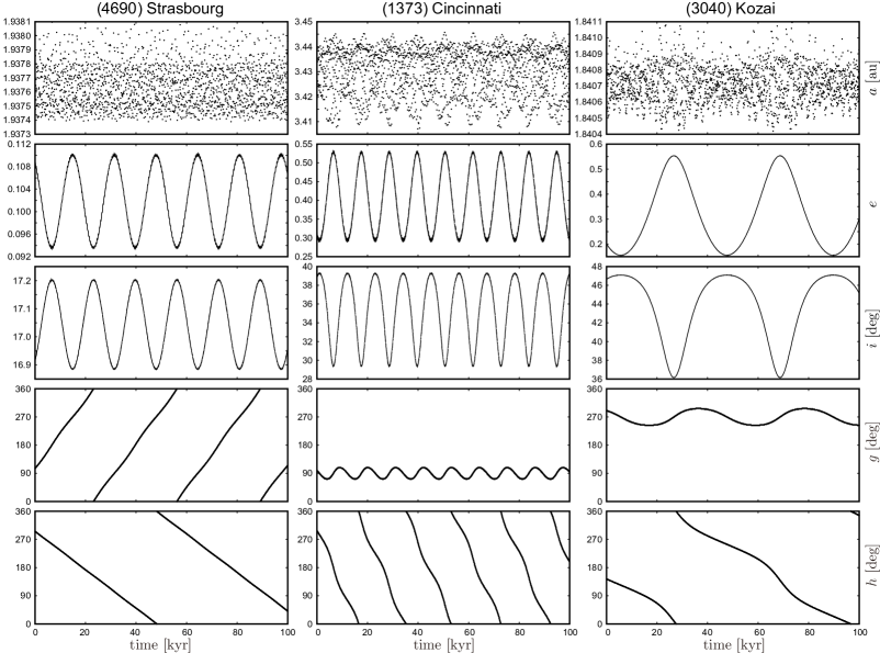
Figure 2: Numerical solutions of the orbital evolution of three asteroid proxies under perturbation from a Jupiter-like planet on a circular orbit. Left: (4690) Strasbourg. Middle: (1373) Cincinnati. Right: (3040) Kozai. From the top row, the object’s $a$, $e$, $i$, $g$, and $h$ are displayed. The initial orbital elements of the asteroid proxies are taken from the JPL Horizons web-interface as of June 7, 2017 (see Supplementary Information 3 for its specific website as well as other relevant information provided by JPL). The perturbing planet has the same mass and the same semimajor axis with Jupiter, but its eccentricity and inclination are both zero.

2.4 Numerical examples

The analytic expression of the disturbing function for CR3BP in Eqs. (26) and (27), in particular their lowest-order term $(n=1)$, plays a central role in the discussions developed in the remainder of this monograph. Before we move on, let us show some numerical examples of CR3BP for giving readers a rough picture of how typical CR3BP systems behave on a long-term, secular timespan.

The first example is a Sun–planet–asteroid system where the perturbing planet has the same mass and the semimajor axis as Jupiter, but its orbital eccentricity ($e^{\prime}$) is zero. We consider the inner problem, and place three asteroid proxies as the perturbed body orbiting inside this Sun–planet binary. They are (4690) Strasbourg, (1373) Cincinnati, and (3040) Kozai. Then we numerically propagate their orbital evolution over 100 kyr ($10^{5}$ years) in the future direction by directly integrating the equations of motion (15), and make a set of plots of their orbital elements (Fig. 2). The nominal stepsize that we use here is 1 day, and the data output interval is 100 years. As for the numerical integrator, we use the Wisdom–Holman symplectic map. We will explain our numerical method later in more detail (Section 3.7).

Among the three sets of panels in Fig. 2, the motion of (4690) Strasbourg shown in the panels at the left exhibits the most typical behavior in the inner CR3BP. We find several noticeable characteristics here:

• Semimajor axis $(a)$ remains almost constant, although it shows a short-term oscillation with a small amplitude.

• Eccentricity $(e)$ and inclination $(i)$ show regular, anti-correlated oscillations. When $e$ becomes large (or small), $i$ becomes small (or large).

• Argument of pericenter $(g)$ circulates in the prograde direction. Its circulation period has a correlation to the $e$–$i$ oscillation.

• Longitude of ascending node $(h)$ circulates in the retrograde direction. Its circulation period does not seem to have particular correlations to $e$, $i$, or $g$.

The first characteristic ($a$ being almost constant) originates from the general fact that the semimajor axis of the perturbed body remains constant in the doubly averaged CR3BP (i.e. $\left<\left<a\right>\right>$ becomes a constant). The second and the third characteristics (the regular and correlated oscillations of $e$, $i$, and $g$) typically exemplify the so-called Lidov–Kozai oscillation in its circulation regime. We will explore the further details of these characteristics in later sections.

On the other hand, the motions of other objects shown in Fig. 2 (the middle and the right panels) look qualitatively different from that of (4690) Strasbourg, although both of them are regular and exhibiting the $e$–$i$ anti-correlated oscillation as well. As for (1373) Cincinnati whose motion is shown in the middle column panels, the argument of pericenter $g$ librates around $\frac{\pi}{2}$, instead of circulating from 0 to $2\pi$. Its oscillation still seems correlated to the $e$–$i$ couple. As for (3040) Kozai whose motion is shown in the right column panels, the argument of pericenter $g$ seems to librate around $\frac{3\pi}{2}$ with a similar correlation.

What makes these differences? The key to understanding things here lies in the difference of their initial orbital inclination. More specifically, the difference of the vertical component of angular momentum matters. Looking at a quantity $\left(1-e^{2}\right)\cos^{2}i$ which is proportional to the square of the vertical component of the perturbed body’s angular momentum, it is $\sim 0.91$ for (4690) Strasbourg. On the other hand it is $\sim 0.55$ for (1373) Cincinnati, and $\sim 0.45$ for (3040) Kozai. Considering the fact that the quantity $\left(1-e^{2}\right)\cos^{2}i$ takes the value between 0 and 1 (as long as the motion is elliptic), at this point we can deduce that the libration of the argument of pericenter seen in the motion of (1373) Cincinnati and (3040) Kozai takes place when the vertical component of the asteroids’ angular momentum is small.

CR3BP is a simple dynamical model. However, it has the capability to explain many of the fundamental properties observed in the actual solar system dynamics. The $e$–$i$–$g$ correlated oscillation seen in Fig. 2 is one of them. For comparison, we carried out another set of numerical propagation of the orbits of (1373) Cincinnati and (3040) Kozai starting from the same initial condition as in Fig. 2, but under the perturbation from all the eight major planets from Mercury to Neptune with their actual orbital elements (we might want to describe it as a restricted “8$+$1” or “8$+$2”-body system). We pick the resulting time series of asteroids’ $a$, $e$, $i$, and $g$ in Fig. 3. Comparing the panels that show the motions of (1373) Cincinnati and (3040) Kozai in Fig. 2 and in Fig. 3, it is obvious that the CR3BP approximation that was employed to draw Fig. 2 largely possesses the dynamical characteristics that the system with the full planetary perturbation (Fig. 3) possesses: The anti-correlated oscillation between $e$ and $i$, the coherent oscillation of $g$ with the $e$–$i$ couple, the libration of (1373) Cincinnati’s $g$ at $\frac{\pi}{2}$, and the libration of (3040) Kozai’s $g$ at $\frac{3\pi}{2}$. Their semimajor axes remain almost constant during the integration period although we see occasional enhancement of the oscillational amplitude of (3040) Kozai’s $a$. This comparison literally tells us that CR3BP is still useful in solar system dynamics in spite of its structural simplicity. It helps us understand the dynamical nature of the motion of various objects that compose hierarchical three-body systems. This is particularly true for long term dynamics where only the secular motion of objects matters.

Before closing this section, we would like to temporarily and intentionally deviate from the scope of this monograph. Let us explore just a little the world of non-circular (eccentric) restricted three-body problem where the perturber’s eccentricity $e^{\prime}$ is not zero. From a theoretical perspective, this case is qualitatively different from CR3BP because the double averaging procedure would not make the system integrable. This means that, the system’s degrees of freedom remain larger than unity even after the double averaging. As a consequence, the dynamical behavior of the system can be very different from CR3BP. As an example, we prepare yet another Sun–planet–asteroid system where the perturbing planet has the same mass and semimajor axis as Jupiter. The difference from the examples shown in Fig. 2 is that we give the perturbing planet a finite eccentricity: $e^{\prime}=0.2$. The perturbed body is a fictitious asteroid whose initial orbital elements are $a=2.80$ au, $e=0.1$, $i=70^{\circ}$, $h=143^{\circ}$, and $g=270^{\circ}=\frac{3\pi}{2}$. Therefore $\left(1-e^{2}\right)\cos^{2}i\sim 0.12$. We numerically propagate the orbital evolution of this three-body system by directly integrating the equations of motion (15), and present the time variation of $a,e,i,g$ of the perturbed asteroid in Fig. 4. In the first 100 kyr of time evolution (the four panels in the left column of Fig. 4), the behavior of the perturbed asteroid is somewhat similar to the CR3BP case: the semimajor axis $a$ remains almost constant except for the occasional and small enhancement of amplitude. the eccentricity $e$ and inclination $i$ have an anti-correlated oscillation. The argument of pericenter $g$’s oscillation is also correlated with the $e$–$i$ couple. $g$ librates around $270^{\circ}$ during this period. However, their oscillation is not as regular as what we saw in Fig. 2. Also, we see that the amplitude of the eccentricity variation is very large. These features become even clearer when we extend the integration period to 2000 kyr (the four panels in the right column of Fig. 4). The most intriguing aspect concerns the oscillation of orbital inclination. Although its oscillation is still anti-correlated to that of the eccentricity $e$, the inclination $i$ frequently and irregularly exceeds $90^{\circ}$. This means that the orbit of the perturbed body flips, and flips back. The amplitude of the eccentricity variation is remarkably large, and the argument of pericenter changes its status between libration and circulation. This kind of behavior is never observed in CR3BP.

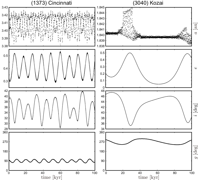
Figure 3: Numerical solutions of the orbital evolution of two asteroids under perturbation from all the eight major planets from Mercury to Neptune. Left: (1373) Cincinnati. Right: (3040) Kozai. From the top row, the object’s $a$, $e$, $i$, and $g$ are displayed. The initial orbital elements of the asteroids are the same as those used in Fig. 2. The planetary masses and initial orbital elements are taken from the JPL Horizons web-interface as of June 7, 2017.

The perturbed body’s stochastic behavior observed in Fig. 4 is typical of the so-called eccentric Lidov–Kozai oscillation. This provides us with many clues about the rich dynamical characteristics that the non-circular (eccentric) restricted three-body problem (ER3BP) has. It also helps us understand certain dynamical structures of the solar and other planetary systems that the simple CR3BP cannot explain. However, ER3BP is clearly out of the scope of this monograph. Also, we must have a firm and rigorous understanding of CR3BP before moving on to the world of ER3BP. Therefore in this monograph we concentrate on the description of CR3BP where the perturbing body is always on a circular orbit $(e^{\prime}=0)$. As a start, we first introduce the classic work of Kozai in the following section.

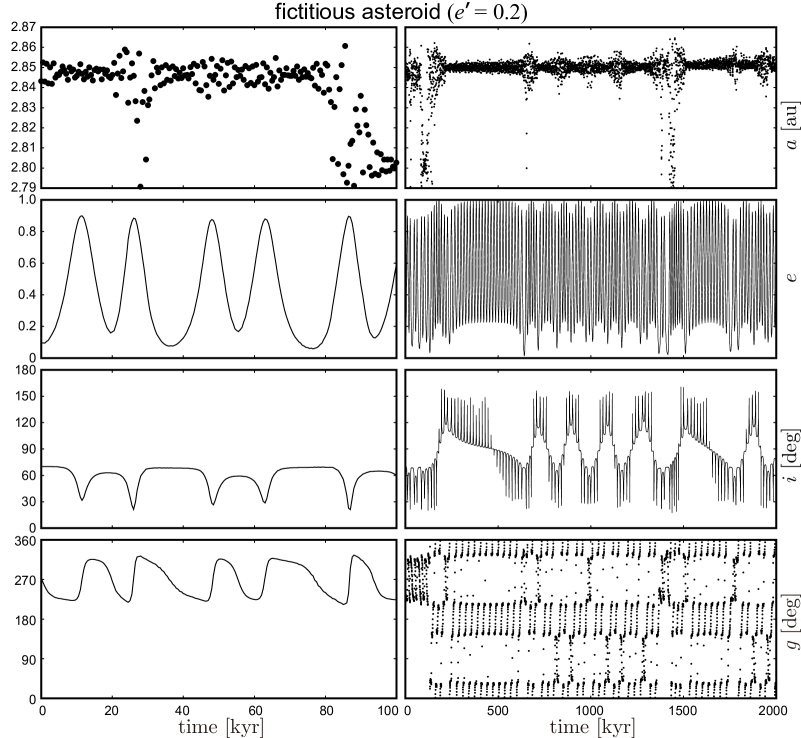
Figure 4: Numerical solutions of the orbital evolution of a fictitious asteroid under perturbation from a Jupiter-like planet on an eccentric orbit $(e^{\prime}=0.2)$. Left: the evolution during the first 100 kyr. Right: the evolution during the entire integration period, 2000 kyr. From the top row, the object’s $a$, $e$, $i$, and $g$ are displayed. The perturbing planet has the same mass and semimajor axis as Jupiter, and its inclination is zero. The initial orbital elements of the asteroid are described in the main text.

3 The Work of Kozai

Yoshihide Kozai (1928–2018) was a Japanese celestial mechanist who is famous for a variety of works on the dynamics of small solar system bodies, planetary satellites, and artificial satellites around the Earth. Several oral history publications are available for Kozai’s research and life, such as DeVorkin (1997, an online publication by American Institute of Physics) or Takahashi (2015a, b, c, d, e, a series of articles written in Japanese with abstracts in English.). More recently, Kozai made a brief summary of his academic career and personal life (Kozai, 2016) including his work on the present subject.

One of Kozai’s achievements that made him renowned was his work on the gravitational potential of the Earth. Through a detailed analysis of artificial satellite motion, Kozai showed that the gravitational potential of the Earth has a non-negligible north-south asymmetry (e.g. Kozai, 1958, 1959a, 1959b, 1959c, 1960, 1961). Another of his achievements that made him famous in astronomy worldwide was his work on the very subject of this monograph: the secular motion of asteroids that have large inclination in the framework of CR3BP. His celebrated work on this (Kozai, 1962) was entitled “Secular perturbation of asteroids with high inclination and eccentricity,” and was published in The Astronomical Journal. The full text of this paper can be accessed through SAO/NASA Astrophysics Data System (hereafter referred to as ADS). This paper deals with a restricted three-body system including the central mass (Sun), a small perturbed body (asteroid), and a large perturbing body (Jupiter) orbiting on a circular orbit. The section structure of Kozai (1962) is as follows: I. Introduction, II. Equations of motion, III. Stationary point, IV. Disturbing function, V. Case for small $\alpha$, VI. Trajectory, and VII. Remarks. This paper was more widely and quickly recognized than any other literature that dealt with a similar subject, and consequently, the influence of this paper on later studies is huge. As a result, the citation frequency of this paper is very high, and is still increasing now (see the descriptions later such as in Section 6.2.3). Kozai (1962) was also selected as one of the 53 “Selected Fundamental Papers Published this Century in the Astronomical Journal and the Astrophysical Journal,” (Abt, 1999).

3.1 Purpose, method, findings

Kozai’s purpose, method, and findings in his work are concisely summarized in his abstract. Though it may be unnecessary for some readers, we reproduce it here:

“Secular perturbations of asteroids with high inclination and eccentricity moving under the attraction of the sun and Jupiter are studied on the assumption that Jupiter’s orbit is circular. After short-periodic terms in the Hamiltonian are eliminated, the degree of freedom for the canonical equations of motion can be reduced to 1.

Since there is an energy integral, the equations can be solved by quadrature. When the ratio of the semimajor axes of the asteroid and Jupiter takes a very small value, the solutions are expressed by elliptic functions.

When the $z$ component of the angular momentum (that is, Delaunay’s $H$) of the asteroid is smaller than a certain limiting value, there are both a stationary solution and solutions corresponding to libration cases. The limiting value of $H$ increases as the ratio of the semimajor axes increases, i.e., the corresponding limiting inclination drops from $39^{\circ}.2$ to $1^{\circ}.8$ as the ratio of the axes increases from 0.0 to 0.95.” (abstract, p. K591)

We will see what each of his points means in what follows. Note that the specific value of “limiting inclination” $(39^{\circ}.2)$ that Kozai mentions in the above third paragraph corresponds to $\cos^{-1}\sqrt{\frac{3}{5}}$, as we will see soon.

The first section (“I. Introduction”) seems like an extended abstract, where Kozai explains more about each of the major points mentioned in the abstract. In the first paragraph of this section, Kozai mentions the fact that conventional perturbation theories such as those exploiting the Laplace coefficients basically assume that the eccentricity and inclination of objects are small. He writes:

“The stability of the solar system has been proved in the sense that no secular change occurs in the semimajor axes of planetary orbits, and that secular changes of the eccentricities and inclinations are limited within certain small domains. However, the classical theory of secular perturbations for the eccentricity and inclination is based on the assumption that the squares of the eccentricity and inclination are negligible. Although this assumption may be reasonable for major planets, it may not be for some asteroids.” (p. K591)

As Kozai wrote in the above, the major planetary orbits exhibit quasi-periodic oscillations with eccentricities and inclinations remaining reasonably small for billions of years (e.g. Ito and Tanikawa, 2002; Batygin and Laughlin, 2008; Laskar and Gastineau, 2009; Batygin et al., 2015). But this is not always the case for the small solar system bodies. In the second paragraph of this section Kozai points this fact out, using some symbolic notations ($A$ or $B$) as follows:

“The assumption in the classical theory means that a term such as $Be^{2}\sin^{2}i\cos 2g$ is negligibly small as compared with the principal term $A(e^{2}-\sin^{2}i)$ in the secular part of the disturbing function. However, as the value of $B$ increases much more rapidly than does that of $A$ with the ratio of the semimajor axes of the asteroid and the perturbing planet, the $B$ term cannot be neglected when the eccentricity and inclination assume large values. For example, the rate of change of the argument of perihelion, which is proportional to $A+B\sin^{2}i\cos 2g$, may vanish at a certain point when the inclination of the asteroid takes a reasonably large value.” (p. K591)

Readers will later encounter more specific expressions of each of the terms in the disturbing function. A point to note in the above paragraph is that, Kozai mentions a possibility for argument of perihelion of an asteroid to stay around a fixed value when its inclination is large enough.

After mentioning a few relevant studies (including Lidov’s work) in the third paragraph of this section, Kozai states his method in the fourth paragraph:

“The present paper treats an analytical theory on secular perturbations of asteroids with high inclination and eccentricity by assuming that only Jupiter, moving in a circular orbit, is the disturbing body. This theory may, of course, be applied also to comets or satellites disturbed by the sun.” (p. K591)

The fifth paragraph is about the advantage of Kozai’s way to expand the disturbing function into a power series of the ratio of semimajor axes, $\alpha$. He writes:

“The conventional technique for developing the disturbing function cannot be adopted here, since neither the eccentricity nor the inclination is considered small. Nor can numerical harmonic analysis be adopted, since variations of orbital elements may not be regarded as small quantities. Therefore, the disturbing function has to be developed into a power series of $\alpha$, the ratio of the semimajor axes of the asteroid and Jupiter, although convergence of the series may be slow.” (p. K591)

The sixth paragraph depicts the possibility to reduce the degrees of freedom of the system by double averaging. This procedure makes the system integrable, and we can then obtain a formal solution by quadrature:

“Short-periodic terms depending on the two mean anomalies can be eliminated from the disturbing function by Delaunay’s transformations. The longitudes of the ascending nodes of Jupiter and the asteroid disappear by the theorem on elimination of nodes. Therefore, the equations of motion for the asteroid are reduced to canonical equations of one degree of freedom with a time-independent Hamiltonian. Therefore, the equations can be solved by a quadrature.” (p. K591)

In the seventh paragraph, after mentioning the existence of an analytic solution of the system expressed by an elliptic function, Kozai states the major conclusion of his work: A stationary solution of $(e,g)$ shows up when a constant parameter $\left(1-e^{2}\right)\cos^{2}i$ is smaller than 0.6:

“In fact, the solutions can be expressed by elliptic functions approximately when $\alpha$ takes a very small value. For this case there are both one stationary and some libration solutions when $\left(1-e^{2}\right)\cos^{2}i$, which is constant, is smaller than 0.6.” (p. K591)

Finally in the eighth paragraph, Kozai states another major conclusion that he obtained: Dependence of the limiting value of $\left(1-e^{2}\right)\cos^{2}i$ for the stationary solutions to exist on the semimajor axes ratio, $\alpha$. Here is what he wrote:

“As $\alpha$ increases, the upper limit of $\left(1-e^{2}\right)\cos^{2}i$ for the existence of a stationary solution increases. When $\alpha$ is 0.85, the limit is as large as 0.90.” (p. K591)

3.2 Equations of motion

Unlike his well-organized abstract and introduction (Section I), we have to say that Kozai’s following four sections (Sections II, III, IV, V) are poorly organized. Not only is it not easy to follow the formulations there, but some descriptions are too terse (or too conceptual) that we do not follow his intention. However, now that most readers are familiar with the method and conclusion of Kozai’s work, let us briefly summarize these sections.

The section “II. Equations of motion” is devoted to describing the canonical equations of motion. In this section Kozai briefly mentions that the doubly averaged CR3BP has just one degree of freedom, and the equations of motion can be solved by quadrature. This section starts from Kozai’s definition of the variables. He denotes $m$ as asteroid’s mass, and $m^{\prime}$ as Jupiter’s mass. The solar mass is set to unity. Kozai uses the Delaunay elements defined as follows:

$$L =\text{k}a^{\frac{1}{2}}, \;\;l =\mbox{ mean anomaly},$$ (K01-45)

$$G =L\left(1-e^{2}\right)^{\frac{1}{2}}, \;\;g =\mbox{ argument of perihelion},$$

$$H =G\cos i, \;\;h =\mbox{ longitude of ascending node},$$

where $l$, $g$, $h$ are the canonical coordinates and $L$, $G$, $H$ are the corresponding conjugate momenta. k is the Gaussian gravitational constant, which is practically equivalent to $\sqrt{{\cal G}}$ that we used in our Section 2 (cf. Brouwer and Clemence, 1961, their p. 57). Note that Kozai’s definition of $L$ in Eq. (K01-45) seems slightly different from those in standard textbooks, $L=\sqrt{\mu a}$ (e.g. Boccaletti and Pucacco, 1996, p. 161), although they are fundamentally equivalent.

Kozai expresses all the quantities of Jupiter with primes such as $L^{\prime}$ and $l^{\prime}$. Also, a variable $\text{k}^{\prime}$ is defined as

$${\text{k}^{\prime}}^{2}=\frac{\text{k}^{2}}{1+m^{\prime}}\frac{{m^{\prime}}^{2}}{m^{2}}=\text{k}^{2}{\mu^{\prime}}^{2}\frac{1+m^{\prime}}{m^{2}},$$ (K02-46)

where $\mu^{\prime}$ is the reduced mass of Jupiter,

$$\mu^{\prime}=\frac{m^{\prime}}{1+m^{\prime}}.$$ (48)

Next, Kozai defines the coordinates of Jupiter with the Sun at the origin, and that of the asteroid with the barycenter of Jupiter and the Sun at the origin. It is nothing but the Jacobi coordinates that we mentioned in Section 2.2, but note that Kozai assumes that the asteroid’s orbit is located inside Jupiter’s orbit (i.e. $r<r^{\prime}$). Then, Kozai expresses the Hamiltonian $F$ of the system as follows:

$$F =\frac{\text{k}^{4}}{2L^{2}}+\frac{m}{\mu^{\prime}}\frac{{\text{k}^{\prime}}^{4}}{2{L^{\prime}}^{2}}$$ (K03-48)

$$\quad+\text{k}^{2}\mu^{\prime}\left\{\left[r^{2}-2rr^{\prime}\frac{s}{1+m^{\prime}}+\left(\frac{r^{\prime}}{1+m^{\prime}}\right)^{2}\right]^{-\frac{1}{2}}\right.$$

$$\quad\quad\left.-\frac{r}{r^{\prime}}\frac{s}{1+m^{\prime}}\right\},$$

where

$$s=\frac{xx^{\prime}+yy^{\prime}+zz^{\prime}}{rr^{\prime}}.$$ (K04-49)

Readers should find the equivalence between the Hamiltonian $F$ in Eq. (K03-48) and ${\cal H}$ in Eq. (32). The third term of the right-hand side of Eq. (K03-48) is not yet expanded into the Legendre polynomials. Since $s$ in Eq. (K04-49) corresponds to $\cos S_{12}$ in Eq. (32) (or $\cos S$ in Eq. (23)), the last term of the right-hand side of Eq. (K03-48) is equivalent to the indirect part of the disturbing function expressed in Eq. (17). Also, keep in mind that the indirect part cancels out with the $P_{1}$ term in the expansion using the Legendre polynomials, as we already saw in Eq. (32).

After expressing the Hamiltonian $F$ in Eq. (K03-48), Kozai tries to reduce the degrees of freedom of the system through two steps. First, Kozai applies “Jacobi’s elimination of the nodes” to the Hamiltonian $F$. It is known that the Hamiltonian in the system considered includes $h$ and $h^{\prime}$ only in the form of $h-h^{\prime}$ (e.g. Nakai and Kinoshita, 1985). By choosing the invariable plane as a reference plane, the Hamiltonian $F$ acquires the rotation symmetry around the total angular momentum vector (e.g. Jacobi, 1843a, b; Charlier, 1902, 1907; Jefferys and Moser, 1966). This circumstance is typically expressed by a relationship

$$h-h^{\prime}=\pi.$$ (51)

This relationship enables us to eliminate both $h$ and $h^{\prime}$ from the Hamiltonian, therefore the conjugate momenta $H$ and $H^{\prime}$ become constants of motion. As a consequence, the original Hamiltonian $F(L,G,H,L^{\prime},G^{\prime},H^{\prime},l,g,h,l^{\prime},g^{\prime},h^{\prime})$ in Eq. (K03-48) with six degrees of freedom is converted into $F(L,G,L^{\prime},G^{\prime},l,g,l^{\prime},g^{\prime})$ with four degrees of freedom.

Note that Kozai actually assumed

$$h=h^{\prime},$$ (K05-51)

as a consequence of Jacobi’s elimination of the nodes, not Eq. (51) that is widely recognized. Eq. (K05-51) certainly eliminates both $h$ and $h^{\prime}$ from the Hamiltonian as long as it contains $h$ and $h^{\prime}$ just in the form of $h-h^{\prime}$, and the conclusion that Kozai stated would not be affected. However, we have not found any expressions similar to Eq. (K05-51) in other literature, and we do not know Kozai’s intention.

The second step that Kozai took in order to reduce the degrees of freedom of the system is double averaging. As we already summarized its concept in Section 2.3, fast-oscillating variables can be eliminated from Hamiltonian by averaging. In the present case, the mean anomalies of asteroid $(l)$ and Jupiter $(l^{\prime})$ can be eliminated. Then their conjugate momenta $L$ and $L^{\prime}$ become constants of motion. As we mentioned in Section 2.3, the elimination of fast-oscillating variables by an averaging procedure is a part of canonical transformation. Therefore Kozai puts a superscript $\ast$ on the variables that have gone through averaging as being canonically transformed. Now, the Hamiltonian $F(L,G,L^{\prime},G^{\prime},l,g,l^{\prime},g^{\prime})$ with four degrees of freedom is transformed into a new Hamiltonian $F^{\ast}(G^{\ast},{G^{\prime}}^{\ast},g^{\ast},{g^{\prime}}^{\ast})$ with two degrees of freedom. Kozai expresses the new Hamiltonian $F^{\ast}$ as follows:

$$F^{\ast}=\frac{\text{k}^{4}}{2{L^{\ast}}^{2}}+m^{\prime}W^{\ast},$$ (K08-52)

with

$$W^{\ast}=\frac{\text{k}^{2}}{4\pi^{2}}\int_{0}^{2\pi}\int_{0}^{2\pi}\frac{1}{\left({r^{\prime}}^{2}-2rr^{\prime}s+r^{2}\right)^{\frac{1}{2}}}dldl^{\prime}.$$ (K09-53)

Note that in the original work by Kozai, the left-hand side of Eq. (K09-53) is $W$, not $W^{\ast}$. However, we believe this is a simple typographic error because the right-hand side of Eq. (K09-53) is doubly averaged, as is the new Hamiltonian $F^{\ast}$ appearing in Eq. (K08-52). Therefore we replace $W$ for $W^{\ast}$ in the following discussion.

$F^{\ast}$ in Eq. (K08-52) does not include the Hamiltonian that drives the Keplerian motion of Jupiter. $W^{\ast}$ in Eq. (K09-53) expresses the perturbation Hamiltonian, but it contains just the direct part of the disturbing function; the indirect part (i.e. the last term of the right-hand side of Eq. (K03-48)) is omitted. Kozai then assumes that Jupiter’s eccentricity is negligibly small, and that its argument of perihelion ${g^{\prime}}^{\ast}$ and its conjugate momentum ${G^{\prime}}^{\ast}$ disappear from $F^{\ast}$. This makes the degrees of freedom unity, and Kozai gives the canonical equations of motion of the asteroid as

$$\frac{dG^{\ast}}{dt}=m^{\prime}\frac{\partial W^{\ast}}{\partial g^{\ast}},\quad\frac{dg^{\ast}}{dt}=-m^{\prime}\frac{\partial W^{\ast}}{\partial G^{\ast}},$$ (K10-54)

with an integral

$$W^{\ast}=\mbox{ const.}$$ (K11-55)

As Kozai writes at the end of this section, in principle we can solve Eq. (K10-54) by quadrature.

3.3 Stationary point

Next in “III. Stationary point,” Kozai gives his estimate on the location of the stationary points that the perturbation part of the doubly averaged Hamiltonian $W^{\ast}$ can have. At these stationary points, $g^{\ast}$ and $e^{\ast}$ (therefore $G^{\ast}$) of the perturbed body are supposed to be constant. What Kozai employs here is a numerical analysis, not an analytical treatment. This is perhaps not what many readers would anticipate him to do.

Kozai first states that, $W^{\ast}$ in Eq. (K09-53) takes the following form when $e^{\prime}=0$:

$$W^{\ast}=\sum_{j=0}A_{j}\left(\alpha,G^{\ast},H\right)\cos 2jg^{\ast},$$ (K12-56)

with

$$\alpha=\left(\frac{\text{k}^{\prime}L^{\ast}}{\text{k}{L^{\prime}}^{\ast}}\right)^{2}.$$ (K13-57)

It is clear that $\alpha$ in Eq. (K13-57) is practically equivalent to the ratio of semimajor axes between the perturbed and perturbing body, $\frac{a}{a^{\prime}}$. Meanwhile $A_{j}$ in Eq. (K12-56) is a coefficient depending on $\alpha$, $G^{\ast}$, and $H$. Kozai did not give any proof of Eq. (K12-56) or specific function form of $A_{j}$ at all at this point. Its function form, however, is revealed in later sections when he presents an analytic expansion of $W^{\ast}$.

Once admitting that the expansion form of Eq. (K12-56) is valid, we can accept Kozai’s statement that $\frac{dg^{\ast}}{dt}$ vanishes when $\sin 2g^{\ast}=0$ owing to the canonical equations of motion (K10-54). More specifically writing, from Eq. (K12-56) and the first equation of Eq. (K10-54) we have

$$\frac{\partial W^{\ast}}{\partial g^{\ast}} =\sum_{j=0}A_{j}\left(\alpha,G^{\ast},H\right)\frac{\partial}{\partial g^{\ast}}\cos 2jg^{\ast}$$ (59)

$$=-\sum_{j=0}2jA_{j}\left(\alpha,G^{\ast},H\right)\sin 2jg^{\ast},$$

which indicates that $\sin 2g^{\ast}=0$ is a condition for $W^{\ast}$ to be stationary somewhere in phase space. $\sin 2g^{\ast}=0$ means $\cos 2g^{\ast}=+1$ or $\cos 2g^{\ast}=-1$. Then, from the second equation of Eq. (K10-54) we get

$$\frac{\partial W^{\ast}}{\partial G^{\ast}}=\sum_{j=0}\frac{\partial A_{j}\left(\alpha,G^{\ast},H\right)}{\partial G^{\ast}}\cos 2jg^{\ast}.$$ (60)

This result means that the considered system has a stationary point under either of the following conditions:

$$\sum_{j=0}\frac{\partial A_{j}}{\partial G^{\ast}} =0\;\;(\mbox{when }\cos 2g^{\ast}=+1),$$ (K14-61)

$$\sum_{j=0}(-1)^{j}\frac{\partial A_{j}}{\partial G^{\ast}} =0\;\;(\mbox{when }\cos 2g^{\ast}=-1).$$ (K15-62)

Here Kozai also puts another inequality

$$H\leq G^{\ast}\leq L^{\ast},$$ (K16-62)

which seems obvious for us because $\sqrt{1-e^{2}}\leq 1$ and $|\cos i|\leq 1$ as long as we consider elliptic orbits.

Table 1: Reproduction of Table I of Kozai (1962, p. K592). The values in the column named as “$i_{0}$” are obtained from Kozai’s “numerical harmonic analysis.” The values in the column named as “$i_{0}$ approx” are from the analytic expansion of $W^{\ast}$ that Kozai accomplished in the later section (see our p. 3.3 for detail). $\left(\frac{H_{0}}{L^{\ast}}\right)^{2}$ is related to $\cos i_{0}$ through Eq. (K17-63). The values of $i_{0}$ that are numerically obtained are later plotted as our Fig. 15 (p. 15) for a comparison with von Zeipel’s achievement.

$\alpha$	$\left(\frac{H_{0}}{L^{\ast}}\right)^{2}$	$i_{0}$	$\begin{subarray}{c}i_{0}\\ {\mathrm{approx}}\end{subarray}$
0.00	0.60 000	$39^{\circ}.231$	$39^{\circ}.231$
0.05	0.60 116	$39^{\circ}.164$	$39^{\circ}.164$
0.10	0.60 464	$38^{\circ}.960$	$38^{\circ}.960$
0.15	0.61 043	$38^{\circ}.620$	$38^{\circ}.620$
0.20	0.61 849	$38^{\circ}.146$	$38^{\circ}.146$
0.25	0.61 880	$37^{\circ}.536$	$37^{\circ}.535$
0.30	0.64 133	$36^{\circ}.791$	$36^{\circ}.790$
0.35	0.65 599	$35^{\circ}.911$	$35^{\circ}.905$
0.40	0.67 274	$34^{\circ}.894$	$34^{\circ}.875$
0.45	0.69 154	$33^{\circ}.738$	$33^{\circ}.694$
0.50	0.71 230	$32^{\circ}.437$	$32^{\circ}.355$
0.55	0.73 495	$30^{\circ}.986$	$30^{\circ}.860$
0.60	0.75 940	$29^{\circ}.374$	$29^{\circ}.239$
0.65	0.78 556	$27^{\circ}.586$	$27^{\circ}.566$
0.70	0.81 330	$25^{\circ}.600$	$25^{\circ}.925$
0.75	0.84 252	$23^{\circ}.380$	$24^{\circ}.410$
0.80	0.87 305	$20^{\circ}.874$	$23^{\circ}.078$
0.85	0.90 488	$17^{\circ}.964$	$21^{\circ}.926$
0.90	0.94 581	$13^{\circ}.460$	$20^{\circ}.963$
0.95	0.99 900	$1^{\circ}.811$	$\cdots$

When $\cos 2g^{\ast}=+1$, Kozai claims that $W^{\ast}$ does not have any stationary points according to his numerical analysis. Literally citing his description:

“It has been proved numerically that Eq. (K14) does not have such a solution except for $H=G^{\ast}=0$ and the equation $dg^{\ast}/dt=0$ has no meaningful solution other than $\sin 2g^{\ast}=0$, at least when $\alpha$ is less than 0.8.” (p. K593)

However, details of Kozai’s numerical analysis are not presented in his paper at all. Note also that we changed the original expression “Eq. (14)” into “Eq. (K14)” in the above citation for clarifying that this equation denotes Eq. (K14-61). We will continue to adopt this manner throughout the rest of this monograph.

When $\cos 2g^{\ast}=-1$, Kozai describes the condition for $W^{\ast}$ to have stationary points as follows:

“Equation (K15) has a solution when $H$ is equal to or smaller than a limiting value $H_{0}$. When $H$ is equal to $H_{0}$, the stationary solution appears at $G^{\ast}=1$. As $H$ decreases, Eq. (K14) has a smaller value of $G^{\ast}$ as the root, and when $H$ is zero, $G^{\ast}=0$ corresponds to the stationary value. When $H$ is equal to $H_{0}$, the corresponding inclination is derived by

$$H_{0}=L^{\ast}\cos i_{0}.$$ (K17-63)

Both $H_{0}$ and $i_{0}$ depend on $\alpha$ and are derived by numerical harmonic analysis of $dW^{\ast}/dG^{\ast}$. The results are given in Table I and as a solid line in Fig. 1.” (p. K593)

For facilitating reader’s understanding of the above quoted part, we have reproduced Kozai’s Table I as our Table 1. By mentioning his results obtained through the analytic expansion of $W^{\ast}$ up to $O\left(\alpha^{8}\right)$ which is not yet presented at this point in his paper, Kozai continues as follows:

“Besides the numerical harmonic analysis, values of $i_{0}$ are derived analytically by developing the disturbing function into power series of $\alpha$ up to the eighth degree, shown in the last column of Table I and as a broken line in Fig. 1. Comparison of the two lines in Fig. 1 shows that the analytical method can provide rather good values for $i_{0}$ up to $\alpha=0.7$.” (p. K593)

We have to say that, we do not feel that there will be many readers who correctly understand Kozai’s logic and intention at this point, as his explanations are lame. Also, the sudden appearance of the result obtained from his own analytic expansion of the disturbing function at this point seems odd. We believe that readers of this monograph who return to this section after going through Kozai’s paper will find that their understanding is much deeper.

Kozai concludes this section with the following paragraph. It mentions an important, quantitative conclusion on the largest value of $i_{0}$ and its dependence on $\alpha$. However, at this point there is no explanation as to how Kozai reached this result, or what kind of value “$39^{\circ}.2$” means:

“In the first approximation, $i_{0}$ and $H_{0}$ do not depend on Jupiter’s mass $m^{\prime}$. The value of $i_{0}$ drops from $39^{\circ}.2$ to $1^{\circ}.8$ as $\alpha$ increases from 0.0 to 0.95. However, there are few asteroids that have $H$ smaller than $H_{0}$. When $\alpha$ is larger than 0.95, there may be a stationary solution for any value of $H$.” (p. K593)

3.4 Disturbing function

In the next section “IV. Disturbing function,” Kozai presents his detailed calculation on the analytic expansion of the disturbing function up to $O\left(\alpha^{2}\right)$. He uses the notation $R$ for the direct part of the disturbing function. Its definition is the same as in our Section 2:

$$R=\frac{\text{k}^{2}m^{\prime}}{\left(r^{2}-2rr^{\prime}s+{r^{\prime}}^{2}\right)^{\frac{1}{2}}}=\frac{\text{k}^{2}m^{\prime}}{r^{\prime}}\sum_{j=0}^{\infty}P_{j}(s)\left(\frac{r}{r^{\prime}}\right)^{j},$$ (K18-64)

where $s$, which is seen in Eq. (K03-48) and is equivalent to $\cos S$ in our Section 2.2, is expressed as

$$s =\cos(f+g)\cos(f^{\prime}+g^{\prime})$$ (K07-65)

$$\quad\quad\quad+\cos i\sin(f+g)\sin(f^{\prime}+g^{\prime}).$$

Note that the expression of $s$ in Eq. (K07-65) is an outcome of the assumption that the reference plane of the system coincides with the perturber’s orbit.

As we mentioned in our Section 2, the $P_{1}$ term can be dropped from Eq. (K18-64). Also, after the averaging procedure using the mean anomaly $l^{\prime}$ of the perturbing body, all the odd-order terms $(j=3,5,7,\ldots)$ disappear if the perturbing body is on a circular orbit $(e^{\prime}=0)$. Hence Kozai describes the major part of the disturbing function $R_{1}$ that is averaged by $l^{\prime}$ as follows:

$$R_{1} =\frac{1}{2\pi}\int_{0}^{2\pi}(R)_{e^{\prime}=0}dl^{\prime}$$ (K19-66)

$$=\frac{\text{k}^{2}m^{\prime}}{a^{\prime}}\sum_{j=0}^{\infty}P_{2j}(s_{1})\left(\frac{r}{a^{\prime}}\right)^{2j}.$$

Recall that $r^{\prime}$ is now equal to $a^{\prime}$, the perturbing body’s semimajor axis. Note also that Kozai did not give any definitions of $s_{1}$ in Eq. (K19-66). We can say it is a symbolic expression for the averaged value of $s$ by the mean anomaly $l^{\prime}$ of the perturbing body such as

$$s_{1}\equiv\frac{1}{2\pi}\int_{0}^{2\pi}sdl^{\prime}=\left<s\right>_{l^{\prime}},$$ (68)

which is practically equivalent to $\left<\cos S\right>_{l^{\prime}}$ seen in our Section 2.2 (see Eq. (38) for comparison). A confusing point in Kozai’s notation here is that, the averaged values of $s$ never actually show up in the form of Eq. (68): They show up in the form of even powers such as $\left<s^{2}\right>_{l^{\prime}},\left<s^{4}\right>_{l^{\prime}},\left<s^{6}\right>_{l^{\prime}},\left<s^{8}\right>_{l^{\prime}}$, but Kozai denotes them as $s_{1}^{2},s_{1}^{4},s_{1}^{6},s_{1}^{8}$.

After introducing Eq. (K19-66), Kozai presents the specific function forms of $s_{1}^{2},s_{1}^{4},s_{1}^{6},s_{1}^{8}$ in Eq. (K20) together with the averaged values of the Legendre polynomials of the corresponding order, $P_{2}(s_{1}),P_{4}(s_{1}),P_{6}(s_{1}),P_{8}(s_{1})$ in Eq. (K21). Kozai did not show the specific definition of $P_{2j}(s_{1})$, but it is as follows:

$$P_{2j}(s_{1})\equiv\left<P_{2j}(s)\right>_{l^{\prime}}=\frac{1}{2\pi}\int_{0}^{2\pi}P_{2j}(s)dl^{\prime}.$$ (69)

We do not reproduce the specific forms of $s_{1}^{2},s_{1}^{4},s_{1}^{6},s_{1}^{8}$ and $P_{2}(s_{1}),P_{4}(s_{1}),P_{6}(s_{1}),P_{8}(s_{1})$ in this monograph because of their complexity. See Eqs. (K20) and (K21) for the detail.

The next step is to average the disturbing function by the mean anomaly $l$ of the perturbed body. Kozai carried this task out using one of the formulas devised by Tisserand (1889, see Eq. (K22) which we do not reproduce here). The resulting doubly averaged disturbing function $W^{\ast}$ is very complicated, but we venture to reproduce it here. First, remark Kozai’s abbreviated notations

$$\theta=\frac{H}{G^{\ast}},\quad\eta=\frac{G^{\ast}}{L^{\ast}}.$$ (K24-69)

It is obvious that $\theta$ is practically equivalent to $\cos i$, and $\eta$ is practically equivalent to $\sqrt{1-e^{2}}$, if we ignore their difference denoted by $\ast$. Using the notations defined by Eq. (K24-69), $W^{\ast}$ becomes up to $O\left(\alpha^{8}\right)$ as

$$W^{\ast}=\frac{\text{k}^{2}}{a^{\prime}}\alpha^{2}\left\{\frac{1}{16}\left[-\left(1-3\theta^{2}\right)\left(5-3\eta^{2}\right)\right.\right.$$

$$\;\left.+15\left(1-\theta^{2}\right)\left(1-\eta^{2}\right)\cos 2g^{\ast}\right]$$

$$\;+\frac{9}{2^{12}}\alpha^{2}\left[\left(3-30\theta^{2}+35\theta^{4}\right)\left(63-70\eta^{2}+15\eta^{4}\right)\right.$$

$$\;-140\left(1-\theta^{2}\right)\left(1-7\theta^{2}\right)\left(1-\eta^{2}\right)\left(3-\eta^{2}\right)\cos 2g^{\ast}$$

$$\;\left.+735\left(1-\theta^{2}\right)^{2}\left(1-\eta^{2}\right)^{2}\cos 4g^{\ast}\right]$$

$$\;+\frac{5}{2^{17}}\alpha^{4}\left[-10\left(5-105\theta^{2}+315\theta^{4}-231\theta^{6}\right)\right.$$

$$\quad\times\left(429-693\eta^{2}+315\eta^{4}-35\eta^{6}\right)$$

$$\;+315\left(1-\theta^{2}\right)\left(1-18\theta^{2}+33\theta^{4}\right)\left(1-\eta^{2}\right)$$

$$\quad\times\left(143-110\eta^{2}+15\eta^{4}\right)\cos 2g^{\ast}$$

$$\;-4158\left(1-\theta^{2}\right)^{2}\left(1-11\theta^{2}\right)\left(1-\eta^{2}\right)^{2}$$

$$\quad\times\left(13-3\eta^{2}\right)\cos 4g^{\ast}$$

$$\;\left.+99099\left(1-\theta^{2}\right)^{3}\left(1-\eta^{2}\right)^{3}\cos 6g^{\ast}\right]$$

$$\;+\frac{175}{2^{28}}\alpha^{6}$$

$$\quad\times\left[7\left(35-1260\theta^{2}+6930\theta^{4}-12012\theta^{6}+6435\theta^{8}\right)\right.$$

$$\quad\times\left(12155-25740\eta^{2}+18018\eta^{4}-4620\eta^{6}+315\eta^{8}\right)$$

$$\;-27720\left(1-\theta^{2}\right)\left(1-33\theta^{2}+143\theta^{4}-143\theta^{6}\right)$$

$$\quad\times\left(1-\eta^{2}\right)\left(221-273\eta^{2}+91\eta^{4}-7\eta^{6}\right)\cos 2g^{\ast}$$

$$\;+396396\left(1-\theta^{2}\right)^{2}\left(1-26\theta^{2}+65\theta^{4}\right)\left(1-\eta^{2}\right)^{2}$$

$$\quad\times\left(17-10\eta^{2}+\eta^{4}\right)\cos 4g^{\ast}$$

$$\;-490776\left(1-\theta^{2}\right)^{3}\left(1-15\theta^{2}\right)\left(1-\eta^{2}\right)^{3}$$

$$\quad\times\left(17-3\eta^{2}\right)\cos 6g^{\ast}$$

$$\;\left.\left.+15643485\left(1-\theta^{2}\right)^{4}\left(1-\eta^{2}\right)^{4}\cos 8g^{\ast}\right]\right\}.$$ (K23-70)

Through our own algebraic manipulation (Ito, 2016), we have confirmed that there is no miscalculation or typographic error in the expansion of $W^{\ast}$ in Eq. (K23-70).

For reference, let us take just the terms in the leading-order $O\left(\alpha^{2}\right)$ out of the expression of $W^{\ast}$ in Eq. (K23-70). Translating $\theta$ and $\eta$ into the standard notations of orbital elements using $e$ and $i$, and using ${\cal G}$ instead of k, and ignoring all $\ast$ from the symbols for simplicity, this quantity becomes

$$W^{\ast}_{O\left(\alpha^{2}\right)}=\frac{{\cal G}}{a^{\prime}}\left(\frac{a}{a^{\prime}}\right)^{2}$$ (72)

$$\quad\times\frac{1}{16}\left[15e^{2}\sin^{2}i\cos 2g-\left(3e^{2}+2\right)\left(3\sin^{2}i-2\right)\right],$$

which we often find in modern literature (e.g. Naoz, 2016, Eq. (15) on p. 448).

Using the leading-order terms of the disturbing function described in Eq. (72), we can write down the canonical equations of motion for $G$ and $g$ as follows:

$$\frac{dG}{dt} =m^{\prime}\frac{\partial W^{\ast}_{O\left(\alpha^{2}\right)}}{\partial g}$$

$$=-\frac{{\cal G}m^{\prime}}{a^{\prime}}\left(\frac{a}{a^{\prime}}\right)^{2}\cdot\frac{15}{8}e^{2}\sin^{2}i\sin 2g,$$ (73)

$$\frac{dg}{dt} =-m^{\prime}\frac{\partial W^{\ast}_{O\left(\alpha^{2}\right)}}{\partial G}$$

$$=\frac{{\cal G}m^{\prime}}{a^{\prime}}\left(\frac{a}{a^{\prime}}\right)^{2}\cdot\frac{3}{8G}\left[\left(5\cos^{2}i-\left(1-e^{2}\right)\right)\right.$$

$$\quad\quad\left.-5\left(\cos^{2}i-\left(1-e^{2}\right)\right)\cos 2g\right].$$ (74)

The set of equations (73) and (74) is a simplified version of the canonical equations of motion whose general form is Eq. (K10-54). They are also seen in conventional literature (e.g. Kinoshita and Nakai, 1999, Eqs. (5) and (6) on their p. 127). Note that we ignored all $\ast$ from the symbols in Eqs. (73) and (74) except for $W^{\ast}_{O\left(\alpha^{2}\right)}$.

In Section 3.3 (p. 3.3 of this monograph) we introduced Kozai’s estimate that $W^{\ast}$ can have stationary points when $\cos 2g^{\ast}=-1$. Let us see where they are located at the $O\left(\alpha^{2}\right)$ level approximation using Eq. (74).

At the stationary points, we have $\frac{dg^{\ast}}{dt}=0$. From Eq. (74), this means

$$10\cos^{2}i-6\left(1-e^{2}\right)=0.$$ (75)

Here let us notify readers that Kozai defined an important parameter in his discussion at the end of his Section IV. It is denoted as $\Theta$, and expressed as follows:

$$\Theta=\left(\frac{H}{L^{\ast}}\right)^{2}.$$ (K26-75)

This variable is roughly equivalent to $\left(1-e^{2}\right)\cos^{2}i$ and a constant, because both $H$ and $L^{\ast}$ are constant as we saw in the previous discussion. Using $\Theta$ in Eq. (K26-75), we can rewrite the condition (75) as follows:

$$\left(1-e^{2}\right)^{2}=\frac{5}{3}\Theta.$$ (77)

Since we have $0\leq\left(1-e^{2}\right)^{2}\leq 1$ as long as we consider elliptic orbits, the condition (77) holds true only when

$$\Theta\leq\frac{3}{5}.$$ (78)

In other words, the doubly averaged disturbing function $W^{\ast}_{O\left(\alpha^{2}\right)}$ in Eq. (72) cannot have stationary points unless the condition (78) is satisfied. Recalling the definition of $\Theta$ in Eq. (K26-75), Eq. (78) means that there is a threshold value of $H$ only below which the system can have stationary points. Kozai designated it as $H_{0}$ (see his p. K593 and p. 3.3 of this monograph), and its actual expression is

$$H_{0}=\sqrt{\frac{3}{5}}L^{\ast},$$ (79)

from Eqs. (K26-75) and (78).

The threshold value $H_{0}$ can be translated into a threshold value of orbital inclination of the perturbed body, $i_{0}$. As we showed before, Kozai defined $i_{0}$ in Eq. (K17-63) as the value that realizes $G^{\ast}=1$. This obviously happens when $e=0$. Kozai also defined the corresponding threshold $\Theta_{0}$ just after Eq. (K26-75). They yield the relationship

$$\Theta_{e=0}=\Theta_{0}=\left(\frac{H_{0}}{L^{\ast}}\right)^{2}=\cos^{2}i_{0}.$$ (80)

Substituting Eq. (79) into Eq. (80), the actual value of $i_{0}$ is calculated as

$$i_{0}=\cos^{-1}\sqrt{\frac{3}{5}}=39.^{\circ}2315205\cdots,$$ (81)

at the $O\left(\alpha^{2}\right)$ approximation. Kozai develops the same discussion at the $O\left(\alpha^{8}\right)$ approximation based on his calculation result, Eq. (K23-70). He writes:

“The limiting value of $H$ is derived from the equation

$$\left(\frac{\partial W^{\ast}}{\partial G^{\ast}}\right)_{\cos 2g^{\ast}=-1,\eta=1}=0,$$

that is

$$-5\Theta+3+\frac{15}{32}\left(-49\Theta^{2}+46\Theta-5\right)\alpha^{2}$$

$$\quad+\frac{175}{512}\left(-297\Theta^{3}+417\Theta^{2}-143\Theta+7\right)\alpha^{4}$$

$$\quad\quad+\frac{18375}{65536}\left(-1573\Theta^{4}+2974\Theta^{3}-1738\Theta^{2}\right.$$

$$\quad\quad\quad\left.+320\Theta-9\right)\alpha^{6}=0,$$ (K25-81)

” (p. K594)

Note that in Eq. (K25-81), all $\Theta$ should be replaced for $\Theta_{0}$ due to the condition $\eta=1$ (or $e=0$).

Kozai then continues:

“Equation (K25-81) gives the limiting value $\Theta_{0}$ corresponding to $H_{0}$ as a function of $\alpha$. When $\alpha$ is zero, $\Theta_{0}$ is equal to 0.6.” (p. K594)

Equation (K25-81) is still complicated, and it is not easy to derive an inverse form such as $\Theta_{0}(i_{0})=f(\alpha)$ where $f$ is some function. It may be possible to solve Eq. (K25-81) as a cubic equation of $\alpha^{2}$, but we do not know how Kozai obtained the list of the values tabulated in his Table I (in the “$i_{0}$ approx” column in Table 1).

Let us symbolically write Eq. (K25-81) as $f_{1}(\alpha,\Theta_{0})=0$. Instead of directly solving Eq. (K25-81), we have made a plot of equi-value contours that $f_{1}(\alpha,\Theta_{0})$ creates on the $(\alpha,\Theta_{0})$ plane (Fig. 5). Among the contours seen in Fig. 5, we marked a particular contour that denotes the region $f_{1}(\alpha,\Theta_{0})=0$ with red. We have confirmed that the values plotted on the red curve in Fig. 5 is consistent with those tabulated in the “$i_{0}$ approx” column in Kozai’s Table I.

The thick red line in Fig. 5, which denotes the approximate analytic solution of Eq. (K25-81), tells us that the threshold inclination $i_{0}$ monotonically decreases from $\cos^{-1}\sqrt{\frac{3}{5}}\sim 39.^{\circ}2$ to much lower values as $\alpha$ increases. This is consistent with Kozai’s statement that we cited on p. 3.3 of this monograph. This fact means that in the doubly averaged inner CR3BP, the larger $\alpha$ gets, the more easily the stationary points of the motion of the perturbed body can take place even with smaller $i$. We will see this feature later again in von Zeipel’s work (Section 5 of this monograph).

3.5 Solution at quadrupole level

In Kozai’s next section “V. Case for small $\alpha$,” he just picks the lowest-order $O\left(\alpha^{2}\right)$ terms of the doubly averaged disturbing function (72), and discusses its characteristics. This is the quadrupole level approximation, and it is valid only when $\alpha\ll 1$. Kozai’s main interest in this section is to derive an analytic, time-dependent solution of orbital elements governed by the doubly averaged disturbing function at the quadrupole level approximation. On the way he gives considerations on possible solutions in several special cases, and in particular, on their trajectory shapes. Frankly speaking, we feel that this part of the section is poorly organized, partly because of too many conversions of variables and too terse literal descriptions. Therefore we just make a brief summary of Kozai’s categorization of trajectories, and return to the same subject again when we introduce Lidov’s work (Section 4 of this monograph).

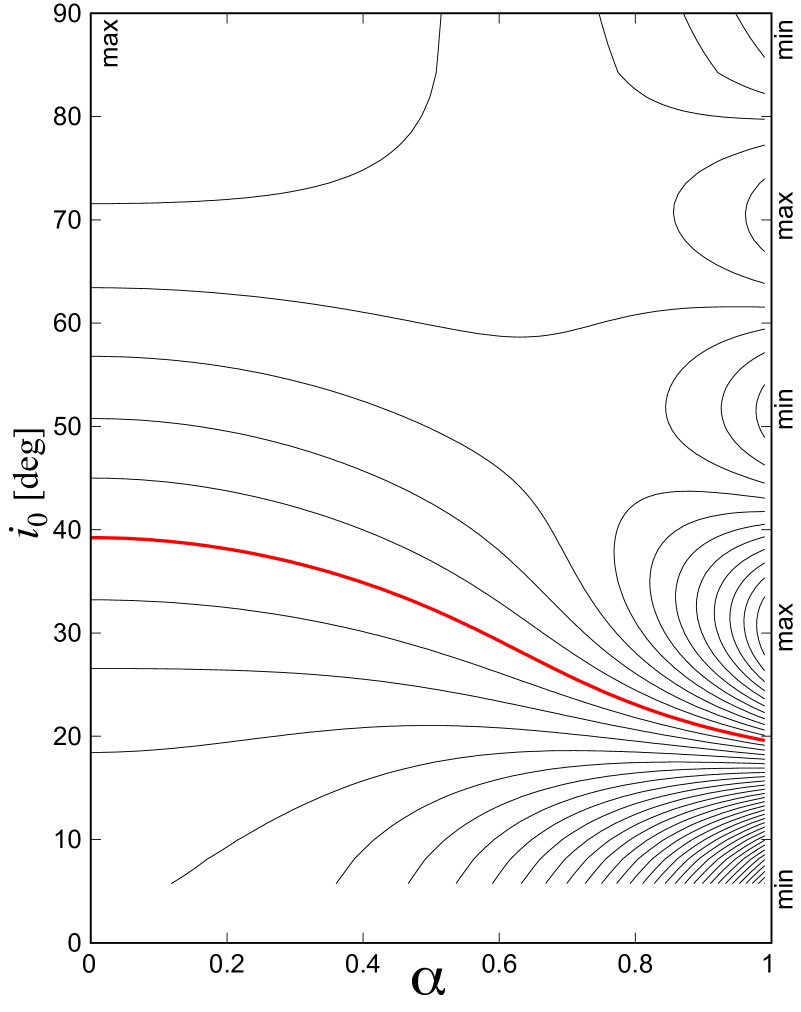
Figure 5: Equi-value contours plotted on the $(\alpha,i_{0})$ plane produced from the left-hand side of Eq. (K25-81). The values of $i_{0}$ are translated from those of $\Theta_{0}$ through Eq. (80). The thick red line indicates the location of the solution of Eq. (K25-81), $f_{1}(\alpha,\Theta_{0})=0$. Note that we have added the labels “min” and “max” near the locations of local minima and local maxima of the function $f_{1}(\alpha,\Theta_{0})$, because it is hard to recognize them just from the grayscale contours.

Kozai begins this section with a simple statement:

“When $a$ is small enough so that we can neglect $\alpha^{2}$ in the braces $\{\}$ in $W^{\ast}$ (K23-70), Eqs. (K10-54) can be integrated by using an elliptic function of Weierstrauss.” (p. K594)

Then Kozai transforms the canonical equation of motion for $\frac{dG^{\ast}}{dt}$ in Eq. (K10-54) into a form that uses different variables. He shows that the energy integral $W^{\ast}$ in Eq. (K11-55) is expressed in the following form

$$-\left(1-\frac{3\Theta}{x}\right)\left(5-3x\right)$$

$$\quad\quad+15\left(1-\frac{\Theta}{x}\right)\left(1-x\right)\cos 2g^{\ast}=C,$$ (K27-82)

with a new variable $x$ defined as

$$x=\eta^{2}.$$ (K28-83)

In other words, $x=1-e^{2}$. He also defines its initial value $x_{0}$ as follows:

$$x_{0}=\left.x\right|_{g^{\ast}=0}.$$ (85)

Then the constant $C$ is expressed by $x_{0}$ and $\Theta$ as

$$C=10-12x_{0}+6\Theta.$$ (K29-85)

Kozai also introduces another variable $y$ as

$$y=3x^{2}-x\left(5+5\Theta-2x_{0}\right)+5\Theta.$$ (K31-86)

Applying Eqs. (K27-82), (K29-85) and (K31-86) to the equation of motion for $\frac{dG^{\ast}}{dt}$ in Eq. (K10-54), Kozai obtains the following ordinary differential equation for $x$:

$$\frac{dx}{dt}=\mp\frac{3}{2}n\alpha^{3}m^{\prime}\sqrt{2\left(x-x_{0}\right)y},$$ (K30-87)

where $n$ is the mean motion of the perturbed body. In the right-hand side of Eq. (K30-87), the negative sign corresponds to the positive values of $\sin 2g^{\ast}$, and the positive sign corresponds to the negative values of $\sin 2g^{\ast}$.

Kozai claims that the solution of the differential equation (K30-87) is categorized into four types, depending on the value of $x_{0}$ (i.e. the initial eccentricity value at $g^{\ast}=0$). Kozai carries this procedure out by solving an equation

$$y=0,$$ (89)

which leads to $\frac{dx}{dt}=0$ from Eq. (K30-87). Let us put brief descriptions of what he wrote for the four cases:

• Case 1. (when $x_{0}=\Theta$)
  In this case, the solution of Eq. (89) is either $x=\Theta$ or $x=\frac{5}{3}$. As $x$ cannot exceed 1, this means $x$ is always equal to $\Theta$. Since $x=1-e^{2}$ and $\Theta=\left(1-e^{2}\right)\cos^{2}i$ by their definitions, $\cos^{2}i$ is always unity. This means that the inclination $i$ of the perturbed body is always zero.

• Case 2. (when $x_{0}=1$)
  In this case, the solution of Eq. (89) is either $x=1$ or $x=\frac{5}{3}\Theta$. If $x=1$, perturbed body is always on a circular orbit $(e=0)$. On the other hand if $x=\frac{5}{3}\Theta$, there is a stationary point at $\cos 2g^{\ast}=-1$ only when $\Theta<\Theta_{0}=\frac{3}{5}$.

• Case 3. (when $\Theta<x_{0}<1$)
  In this case, one of the solutions of Eq. (89) lies in the range of $\Theta\leq x\leq 1$, and the other is $x>1$ (which is not valid). This case embraces the most ordinary trajectories where $g^{\ast}$ makes a circulation from 0 to $2\pi$.

• Case 4. (when $x_{0}>1$)
  In this case, both the solutions of Eq. (89) lie in the range of $\frac{5}{3}\Theta\leq x\leq 1$. So a dynamically meaningful solution can exist only when $\Theta<\Theta_{0}=\frac{3}{5}$. However, $x$ cannot exceed 1 by its definition (K28-83), neither can $x_{0}$ by its definition (85). Therefore we do not exactly understand Kozai’s assumption $(x_{0}>1)$ in this case.

After these categorization of characteristic solutions, Kozai slightly changes the course of discussion. He begins introducing time-dependent analytic solution of the equations of motion expressed by an elliptic function. First, Kozai makes the following statement:

“In each case Eq. (K30-87) can be solved by an elliptic function of Weierstrauss $\wp$,” (p. K595).

More specifically, Kozai introduces another set of variable conversions $(x,t)\to(z,t^{\ast})$ as

$$z =x-\frac{5}{9}\left(1+\Theta\right)-\frac{1}{9}x_{0},$$ (K38-89)

$$t^{\ast} =-\frac{3\sqrt{6}}{4}nm^{\prime}\alpha^{3}t,$$

and he converts the differential equation (K30-87) into the following one:

$$\frac{dz}{dt^{\ast}}=\pm\sqrt{4\left(z-z_{0}\right)\left(z-z_{1}\right)\left(z-z_{2}\right)},$$ (K39-90)

where

$$-z_{0} =z_{1}+z_{2}$$ (K41-91)

$$=\frac{5}{9}\left(1+\Theta\right)-\frac{8}{9}x_{0},$$

$$z_{1}z_{2} =-\frac{50}{81}\left(1+\Theta\right)^{2}$$

$$\quad\quad+\frac{25}{81}x_{0}\left(1+\Theta\right)+\frac{7}{81}x_{0}^{2}+\frac{5}{3}\Theta.$$

Then Kozai says that solution of Eq. (K39-90) can be expressed using Weierstrass’s elliptic function $\wp$ as

$$z=\wp(t^{\ast}).$$ (K40-92)

Consult Southard (1965) or Weisstein (2017) for more detailed information on the function $\wp$.

Note that the original Eqs. (K38-89) and (K41-91) contain typographic errors in Kozai (1962), and we have already rectified them in the above: The original Eq. (K38-89) has $+\frac{1}{9}x_{0}$ instead of the correct $-\frac{1}{9}x_{0}$ in its right-hand side. Also, the second equation of the original Eq. (K41-91) has $+\frac{5}{81}x_{0}\left(1+\Theta\right)$ instead of the correct $+\frac{25}{81}x_{0}\left(1+\Theta\right)$ in its right-hand side. Hiroshi Kinoshita kindly notified us of the typographic errors, and we have confirmed the correctness of this information through our own algebra.

The solution $z$ of the differential equation (K40-92) must be translated into the solution $x$ of Eq. (K30-87) as $x(t^{\ast})$. $x(t^{\ast})$ is supposed to express the time-dependent solution of $e$ as $e(t^{\ast})$. Then, the solution for $g^{\ast}$ is subsequently obtained from Eqs. (K27-82) and (K29-85) as

$$\cos 2g^{\ast}=\frac{Q(x)}{5\left(x-\Theta\right)\left(1-x\right)},$$ (K42-93)

where

$$Q(x)=-x^{2}+\left[5\left(1+\Theta\right)-4x_{0}\right]x-5\Theta.$$ (K43-94)

We can obtain the time-dependent solution for $i$ from the conservation of $\Theta$ such as

$$i=\cos^{-1}\frac{H}{G^{\ast}}.$$ (K44-95)

Note again that the original Eq. (K43-94) in Kozai (1962) contains a typographic error: The first term of the right-hand side of the original Eq. (K43-94) is expressed as $x^{2}$, as opposed to the correct $-x^{2}$. This information was also communicated by Hiroshi Kinoshita.

Kozai also gives a set of differential equations for obtaining time-dependent solutions for the mean anomaly $l^{\ast}$ and the longitude of ascending node $h^{\ast}$ of the perturbed body. They are as follows:

$$\frac{dl^{\ast}}{dt} =n+\frac{3}{8}\frac{nm^{\prime}\alpha^{3}}{\eta}\left(x-3\Theta-\frac{Q(x)}{1-x}\right),$$ (K45-97)

$$\frac{dh^{\ast}}{dt} =-\frac{3}{8}\frac{nm^{\prime}\alpha^{3}\theta}{\eta}\left[5-3x-5\left(1-x\right)\cos 2g^{\ast}\right]$$

$$=-\frac{3}{8}\frac{nm^{\prime}\alpha^{3}\theta}{\eta}\left[5-3x-\frac{Q(x)}{x-\Theta}\right].$$ (K46-98)

Note that Kozai uses the variable $t$ in the left-hand side of Eqs. (K45-97) and (K46-98) instead of $t^{\ast}$. Also, although we guess that he reached these solutions through analytic quadrature, there is no mention of the detail as to how Kozai derived Eqs. (K45-97) and (K46-98). Readers can consult later studies along this subject for more detail (e.g. Vashkov’yak, 1999; Kinoshita and Nakai, 2007). There is also a short discussion about this subject later in this monograph (Section 6.1.1 on p. 6.1.1).

3.6 Equi-potential trajectories

We presume that one of the features that makes Kozai’s work a historic standard is his use of the so-called equi-potential contours described in his section “VI. Trajectory.” Drawing equi-potential contours (trajectories) of the averaged disturbing function helps us grasp a global picture of the perturbed body’s motion in phase space without actually seeking specific time-dependent solutions. On diagrams with equi-potential contours, we can see the existence or non-existence of stationary points, the oscillating amplitude of orbital elements, and the location of separatrix if any, at a glance. Kozai describes what he did as follows:

“Trajectories of Eqs. (K10-54) can be plotted on the $\left(2g^{\ast},1-e^{2}\right)$ plane by using the energy integral $W^{\ast}$ (K23-70). In Figs. 2 through 5 the trajectories are shown for $\alpha=0$.” (p. K596)

Needless to say, this procedure is possible because the doubly averaged CR3BP has just one degree of freedom, and because the energy integral $W^{\ast}$ (K23-70) itself is constant. We reproduced Kozai’s Figs. K2, K3, K4, K5, and K8 as the left column panels of our Fig. 6. Note that Kozai did not mention anything on his Fig. K8 in his paper. We do not know why, and we have no idea either as to why only Fig. K8 is isolated, placed beyond Figs. K6 and K7.

Kozai’s Fig. K2 (corresponding to our reproduction shown in the top panel in the left column of Fig. 6) is for a system with $\Theta=0.8$ where stationary points would not show up at the quadrupole level approximation. All the trajectories exhibit circulation of $2g^{\ast}$ from 0 to $2\pi$. Note that Kozai added arrows on each of the contours in his original figures so that readers can understand the direction of motion. Our reproduction does not include these arrows.

Kozai’s Fig. K3 (corresponding to our reproduction shown in the second panel from the top in the left column of Fig. 6) is for a system with $\Theta=0.6$, the limiting value that changes the dynamical characteristics of the system at the quadrupole level approximation. Past the limiting value, we come to visually recognize stationary points on the diagram. An example result with $\Theta=0.5$ is presented in Kozai’s Fig. K4 (corresponding to our reproduction shown in the third panel from the top in the left column of Fig. 6). In Kozai’s original Fig. K4, it is noticeable that one of the contours reaches the upper boundary of the panel where $x=1-e^{2}=1$. This means that this contour denotes a separatrix of the motion. Note that our reproduction in Fig. 6 does not have an explicit separatrix on it because of the automatic choice of contour interval by the plotting application that we used. The existence of stationary points and the separatrix get more obvious as $\Theta$ gets smaller. An example result when $\Theta=0.3$ is presented in Kozai’s Fig. K5 (corresponding to our reproduction shown in the fourth panel from the top in the left column of Fig. 6).

In Kozai’s Figs. K4, K5, and K8, he added the boundaries where $\frac{dg^{\ast}}{dt}=0$ as broken lines. We reproduced the boundaries in red in the corresponding panels of Fig. 6. Here is how Kozai calculated the location of the boundaries. From the canonical equation of motion for $g^{\ast}$ (74) at the quadrupole level approximation, $\frac{dg^{\ast}}{dt}$ vanishes when the following relationship is satisfied:

$$\cos 2g^{\ast}=\frac{5\Theta-x^{2}}{5\left(\Theta-x^{2}\right)}.$$ (K36-98)

Eq. (K36-98) yields the condition that realizes $\frac{dg^{\ast}}{dt}=0$ as

$$x=\sqrt{\frac{5\Theta\left(1-\cos 2g^{\ast}\right)}{1-5\cos 2g^{\ast}}}.$$ (100)

Equation (100) denotes the location of the boundaries on the $(2g^{\ast},x)$ plane shown in Fig. 6.

Kozai also gave the maximum oscillation amplitude of $2g^{\ast}$ utilizing Eq. (K36-98). When $\Theta<\frac{3}{5}$ and the doubly averaged disturbing function has stationary points, $g^{\ast}$ librates between the two points that realize $\frac{dg^{\ast}}{dt}=0$ centered at $2g^{\ast}=\pi$. At these two points, $2g^{\ast}$ is bound by the condition (K36-98). And from the function form of Eq. (K36-98), the smallest value of $2g^{\ast}$ (or the largest value of $\pi-2g^{\ast}$) takes place when $x^{2}=1$. Substitution of $x^{2}=1$ into Eq. (K36-98) yields the largest oscillation amplitude of $2g^{\ast}$ centered at $2g^{\ast}=\pi$ as

$$2\left(\pi-\cos^{-1}\frac{5\Theta-1}{5\left(\Theta-1\right)}\right).$$ (K37-100)

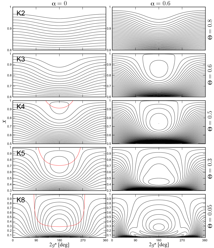
Figure 6: Equi-potential contours of the doubly averaged disturbing function for the inner CR3BP calculated through the analytic expansion that Kozai (1962) gave. The horizontal axis is $2g^{\ast}$, and the vertical axis is $x=1-e^{2}$. The five panels in the left column are the results assuming $\alpha=0$ with $\Theta=0.8,0.6,0.5,0.3,0.05$. They are reproductions of Kozai’s original figures (Figs. K2, K3, K4, K5, K8) where only the lowest-order terms of Kozai’s expansion (K23-70) is included. The red lines in the bottom three panels indicate the location where $\frac{dg^{\ast}}{dt}=0$ is realized. On the other hand, the five panels in the right column are those when $\alpha=0.6$ for the same values of $\Theta$. We placed them for comparison with the panels in the left column. In this case all the terms appearing in Kozai’s expansion (K23-70) up to $O\left(\alpha^{8}\right)$ are used. Note that the smallest value of $x$ is always equal to $\Theta$. This is evident from their definitions ($x=1-e^{2}$, and $\Theta=x\cos^{2}i$) and the fact that the minimum of $x$ is realized when $\cos^{2}i=1$, i.e. when $x=\Theta$.

In Fig. 6, we can visually confirm some of the characteristic trajectories that Kozai categorized in his previous section (see p. 3.5 of this monograph). Case 1 $(x_{0}=\Theta)$ which corresponds to the status of $i=0$ is realized at the lower boundaries of the panels in Kozai’s Figs. K2, K3, K4, K5, K8. As $\Theta=\left(1-e^{2}\right)\cos^{2}i$ is a constant, $i=0$ automatically means that $e$ takes its maximum and also is a constant. Since $x=1-e^{2}$, this trajectory occupies the lower boundary of each panel.

As for Case 2 $(x_{0}=1)$, particularly when $x=1$, the perturbed body is always on a circular orbit $(e=0)$. Therefore the inclination $i$ is also a constant. This trajectory corresponds to the upper boundary of each of the panels, as $x=1$ is its maximum value. Note that when $\Theta<\frac{3}{5}$, the upper boundary of $x=1$ is divided into two parts: where $2g^{\ast}$ circulates from 0 to $2\pi$, and where $2g^{\ast}$ librates with the amplitude given by Eq. (K37-100). Hence it can be misunderstood that the upper boundary of the $(2g^{\ast},x)$ diagram composes a singularity, but it is not. Citing Kozai’s words:

“Two bifurcation points on a line $x=1$ are not actual singularities since they disappear when the coordinates are transformed into polar ones $(e,g^{\ast})$. In fact, for $x=1$, the circular orbit, $g^{\ast}$ cannot be defined. At the bifurcation points $\frac{dg^{\ast}}{dt}$ vanishes.” (p. K596)

Note that what Kozai refers to as “the bifurcation points” above are the contact points of the separatrix and the upper boundary of the panels.

In relation to his Figs. K4, K5, and K8, Kozai left a description on the circumstance when $\Theta$ is small:

“As the value of $\Theta$ decreases, the libration region becomes wide. Even when $\Theta$ is zero, there are trajectories of both libration and complete revolution. For an extreme case the orbit oscillates between a circular perpendicular one and a parabolic one of zero inclination. Although the assumption $\alpha=0$ may not be valid for this case, the results may confirm Lidov’s numerical work (1962).” (p. K597)

It is interesting that Kozai cites Lidov’s numerical work here. We will mention this issue later in this monograph (Section 6.2.4 on p. 6.2.4). As for the $\Theta=0$ case, see Lidov’s discussion that we summarize in Section 4.8 of this monograph (p. 4.8).

When making his Figs. K2, K3, K4, K5, K8, Kozai assumed $\alpha\ll 1$. This is equivalent to the quadrupole level approximation that ignores all the higher-order terms than $O\left(\alpha^{2}\right)$ in the disturbing function. When the higher-order terms in the disturbing function are included, the limiting value of $\Theta$ as well as the shape of the equi-potential trajectories change. This is what Kozai previously mentioned in “III. Stationary point” (see p. 3.3 of this monograph). He describes it again as follows:

“As the value of $\alpha$ increases, for a fixed value of $\Theta$, amplitudes of $x$ become large and the libration region expands as is expected.” (p. K597)

By comparing the panels in the left column (for $\alpha=0$) and those in the right column (for $\alpha=0.6$) in Fig. 6, we can easily see that Kozai’s above statement is true.

There is a point to notice in the bottom right panel of Fig. 6 which is for $(\alpha,\Theta)=(0.6,0.05)$. In this panel we recognize several local extremums in the region of $x\lesssim 0.1$ along $2g^{\ast}=180^{\circ}$, in addition to the major local minimum located around $(2g^{\ast},x)=(180^{\circ},0.25)$. We presume they are artificial features, not real. $x\sim 0.1$ means $e\sim 0.95$. It is known that the analytically expanded doubly averaged disturbing function for CR3BP can sometimes give spurious local extremums when the eccentricity of the perturbed body is very large, even if its truncation order is as high as $\alpha^{8}$ (e.g. Ito, 2016). The apparent local extremums seen in this panel are probably one of these.

3.7 Actual asteroids

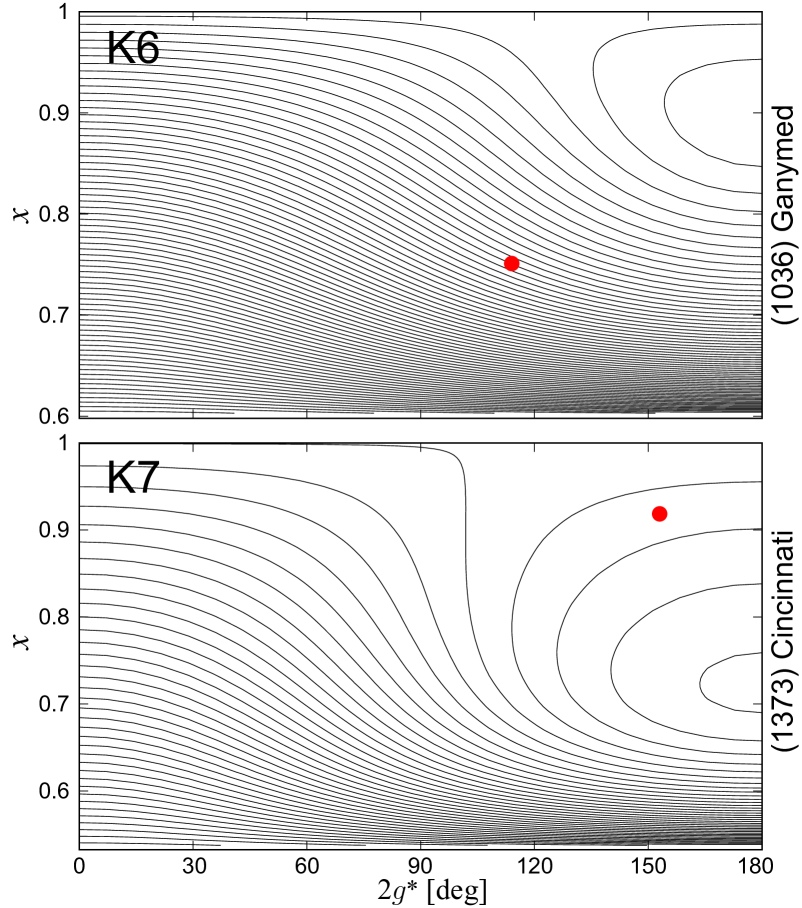
Figure 7: Reproduction of Kozai’s Figs. K6 (upper) and K7 (lower). The upper panel shows the equi-potential contours of the doubly averaged disturbing function for an asteroid (1036) Ganymed, and the lower panel shows that for another asteroid (1373) Cincinnati. They are calculated through the analytic expansion of the doubly averaged disturbing function up to $O\left(\alpha^{8}\right)$ presented in Eq. (K23-70). The axes are common to Fig. 6 except that the range of $2g^{\ast}$ is just between 0 and $180^{\circ}$ (following Kozai’s way). The parameters $\Theta$ and $\alpha$ are adopted from Kozai’s description: $(\Theta,\alpha)=(0.5979,0.5123)$ for Ganymed, and $(\Theta,\alpha)=(0.5325,0.6569)$ for Cincinnati. The red points in each of the panels indicate the “present” location of the asteroids that Kozai mentioned: $(2g^{\ast},x)=(246^{\circ},0.7510)$ for Ganymed, and $(2g^{\ast},x)=(207^{\circ},0.9184)$ for Cincinnati. However, note that the actual location of the asteroids’ $2g^{\ast}$ in these panels are not the written values, but $114^{\circ}(=360^{\circ}-246^{\circ})$ for Ganymed, and $153^{\circ}(=360^{\circ}-207^{\circ})$ for Cincinnati. This is also what Kozai did in his paper.

Kozai then moves on to drawing equi-potential contours for actual objects in the solar system. His objects are two asteroids, (1036) Ganymed and (1373) Cincinnati, whose $\alpha$ values are not negligibly small $(\alpha>0.5)$.

Kozai presented the resulting equi-potential plots in his Figs. K6 and K7 (p. K597), and we reproduce them in our Fig. 7. His description on the motion of these asteroids are short. As for (1036) Ganymed, he writes:

“It is not in the libration region. The eccentricity and inclination oscillate, respectively, between 0.3 and 0.55 and between $23^{\circ}$ and $48^{\circ}$, whereas the present values are 0.5 and $27^{\circ}$.” (p. K597)

This means that, while the doubly averaged disturbing function for Ganymed has a stationary point, its argument of perihelion does not actually librate, but circulates. On the other hand as for (1373) Cincinnati, Kozai writes:

“The present values of the eccentricity and inclination are, respectively, 0.29 and $42^{\circ}$. and they oscillate between 0.25 and 0.6 and between $25^{\circ}$ and $42^{\circ}$. The motion of the argument of perihelion is limited between $60^{\circ}$ and $120^{\circ}$.” (p. K597).

Note that the period placed in “0.29 and $42^{\circ}$. and they $\cdots$’ must be Kozai’s typographic error. It should be replaced for a comma as “0.29 and $42^{\circ}$, and they $\cdots$ .”

Kozai’s above description on (1373) Cincinnati is now considered to be the first “discovery” of a small solar system body whose argument of pericenter librates (Marsden, 1999). The behavior difference between the two asteroids, although their disturbing potentials both have stationary points (local minima) as seen in the right edge of Fig. 7, comes from the difference of the asteroids’ initial orbital energy. Kozai did not explicitly mention this point. The libration of Cincinnati’s $g$ was later confirmed by a direct numerical integration of equations of motion including perturbation from four giant planets and Pluto (Marsden, 1970, p. 210, although no figure or table was given).

At this point let us somewhat deviate from what Kozai achieved, and let us reproduce his result through a different method in different coordinates. This is to confirm the correctness and accuracy of Kozai’s analytic theory.

As for the method, we resort to numerical quadrature defined in Eq. (K09-53). Numerical quadrature is expected to yield a more accurate result than a truncated analytic expansion of the disturbing function, particularly when $\alpha$ is large. Technically speaking, by using the fact that perturber’s orbit is circular in CR3BP, we can turn the double integral (K09-53) into a single integral by employing the complete elliptic integral of the first kind (e.g. Bailey, 1983; Quinn et al., 1990; Bailey et al., 1992). This conversion makes the quadrature (K09-53) faster and more accurate. Our numerical quadrature including the calculation of the elliptic integral was achieved using the functions implemented in GNU Scientific Library (Galassi et al., 2009, GSL 1.16). Note that as we already mentioned on p. 3.3, Kozai himself seemed to carry out the numerical quadrature under the name of “numerical harmonic analysis.” Kozai wrote that he used it for calculating the values listed in his Table K1.

As for the coordinate system, we use polar coordinates $\left(e\cos g^{\ast},e\sin g^{\ast}\right)$ instead of Kozai’s rectangular coordinates $\left(2g^{\ast},1-e^{2}\right)$. The polar coordinates of this type have several advantages over rectangular coordinates. First, periodic trajectories appear as closed curves, not being intersect by diagram borders which happens with rectangular coordinates. Second, the $e=0$ area is represented by a single point at the origin $(0,0)$, and not extended into a line as in rectangular coordinates. Since $g^{\ast}$ is an angle that intrinsically rotates, we believe that the polar coordinates of this type are more appropriate in this problem than rectangular coordinates. The polar coordinates of this type have often been used in prior literature along these lines (e.g. Froeschlé et al., 1991; Michel and Thomas, 1996; Michel and Froeschlé, 1997; Michel, 1997; Michel et al., 1998; Hamilton and Krivov, 1997; Wan and Huang, 2007). We can also regard the coordinates $\left(e\cos g^{\ast},e\sin g^{\ast}\right)$ as a variant of Poincaré coordinates (e.g. Šubr and Karas, 2005; Chenciner, 2015). A disadvantage of using this type of coordinates is that, equi-potential contours sometimes get too crowded and difficult to see in the large $e$ region near the outer boundary. Rectangular coordinate diagrams such as $\left(2g^{\ast},1-e^{2}\right)$ or $\bigl{(}g^{\ast},\sqrt{1-e^{2}}\bigr{)}$ have an advantage in this case. Later in this monograph we will show some of our calculation results in the $\bigl{(}g^{\ast},\sqrt{1-e^{2}}\bigr{)}$ rectangular coordinates (p. 25). Note that in what follows in this monograph, we write $g^{\ast}$ just as $g$ for simplicity. Therefore, the coordinate system we most often employ in this monograph is $\left(e\cos g,e\sin g\right)$.

We chose three asteroids as examples of our demonstration: (1036) Ganymed, (1373) Cincinnati, and (3040) Kozai. As we have seen, Ganymed and Cincinnati are what Kozai dealt with. (3040) Kozai is what we dealt with in our Fig. 2 (p. 2). Incidentally, (3040) Kozai was named after Yoshihide Kozai. The name was proposed by James G. Williams who found that the argument of perihelion of this asteroid is in libration. See MPC (Minor Planet Circulars) 9770 (1985 July 2) and Milani et al. (1989) for more detail. Note also that Milani et al. (1989, in his abstract) introduced the term “Kozai class,” and used it for the objects whose orbital behavior seems to “be protected from node crossing by secular resonances and $e$–$\omega$ coupling (Kozai class).”

We show our calculation results in Fig. 8. The trajectories seen in the upper three panels a, b, c are those obtained through Kozai’s analytic expansion of the doubly averaged disturbing function up to $O\left(\alpha^{8}\right)$, Eq. (K23-70). The trajectories seen in the lower three panels d, e, f are those obtained from the numerical quadrature. Overall, these two sets of equi-potential contours look very similar, indicating the high accuracy of Kozai’s analytic theory. We may see a small discrepancy in the locations of the equilibrium points for (1373) Cincinnati along the direction of $g=\pm\frac{\pi}{2}$ (the panels a and d). This kind of discrepancy would possibly be eliminated if we use even higher-order analytic expansions of the disturbing function than $O\left(\alpha^{8}\right)$.

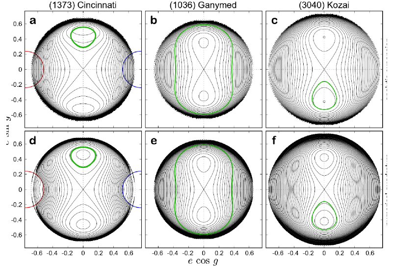
Figure 8: The equi-potential trajectories of three asteroids plotted on the $(e\cos g,e\sin g)$ plane in the CR3BP framework. Top (a, b, c): Equi-potential contours calculated through the analytically expanded doubly averaged disturbing function up to $O\left(\alpha^{8}\right)$ presented in Eq. (K23-70). Bottom (d, e, f): Equi-potential contours calculated through numerical quadrature defined in Eq. (K09-53). a and d are for (1373) Cincinnati, b and e are for (1036) Ganymed, and c and f are for (3040) Kozai. Consult the caption of Fig. 7 as for the $(\Theta,\alpha)$ values of (1373) Cincinnati and (1036) Ganymed. (3040) Kozai’s values used here are $(\Theta,\alpha)=(0.452,0.354)$. The green dots are the actual trajectories of the asteroids obtained through direct numerical integration of the equations of motion. Note that the green numerical trajectories shown in the panel set (a, b, c) and those in the panel set (d, e, f) are identical. In the numerical integration, the initial values of the asteroids’ orbital elements are taken from the JPL Horizons web-interface as of February 16, 2016. The initial locations of each of the asteroids are as follows: $(e,g)=(0.3151321,99^{\circ}.948105)$ for Cincinnati, $(e,g)=(0.5338748,129^{\circ}.934759)$ for Ganymed, and $(e,g)=(0.2005303,288^{\circ}.967682)$ for Kozai. Note also that the numerical data for (1373) Cincinnati and (3040) Kozai is equivalent to what was used in Fig. 2, except that the integration period is longer here (5 million years). The red and the blue partial circles in a and d represent the conditions where the orbits of the perturbed and perturbing bodies intersect each other at the ascending node (red) and at the descending node (blue) of the perturbed body. The black dashed circles represent the theoretically largest eccentricity of the perturbed body in each system. See Section 5.5 for more rigorous definitions of the red and blue partial circles as well as the black dashed circles.

We see red and blue partial circles in the panels for (1373) Cincinnati (a and d). As we will see in more detail later (Sections 5.5 and 5.8 of this monograph), they correspond to the condition of orbit intersection where the orbits of the perturbing and perturbed bodies intersect each other. The disturbing function becomes non-holomorphic on these lines, and they form a set of borders on the $\left(e\cos g,e\sin g\right)$ plane. The numerical quadrature (the panel d) clearly yields these borders, while the analytic expansion of the disturbing function (the panel a) does not. This difference typically shows the limitation of the simple analytic expansion of the disturbing function in this type. The line of orbit intersection in the panels e and f are out of the panel ranges, and we do not have any visual confirmations.

For comparing the equi-potential trajectories that the doubly averaged disturbing function creates with what the actual, unaveraged “raw” CR3BP yields, we carried out a set of direct numerical integration of the equations of motion of these three asteroids. The equations of motion we integrated correspond to Eq. (15) in Section 2 (see p. 15 of this monograph). The system we considered includes asteroids (as mass-less particles), the Sun with its current mass, and Jupiter with its current mass on a circular orbit with semimajor axis $a^{\prime}=5.2042$ au. As for the numerical integration scheme, we employed the so-called Wisdom–Holman symplectic map (Wisdom and Holman, 1991, 1992) implemented as the SWIFT package (Levison and Duncan, 1994). We have modified this code and used it in our previous works (e.g. Strom et al., 2005; Ito and Malhotra, 2010), so we can be assured of the correctness of our numerical integration. The nominal stepsize of the numerical integration here is 1 day, and the total integration time is 5 million years with a data output interval of 500 years.

The resulting numerical trajectories are shown as green dots in each of the panels of Fig. 8. Overall they seem well suited on the equi-potential contours obtained from the doubly averaged disturbing function. Here, let us recall several characteristic features exhibited in Fig. 2 (p. 2). Among the features, the coupled oscillation of $e$ and $g$ is reasonably explained by the trajectories that the green dots make on Fig. 8. The coupling of $e$ and $i$ is now obvious from the fact that $\Theta=\left(1-e^{2}\right)\cos^{2}i$ remains constant in the doubly averaged CR3BP as we saw in Section 3.4.

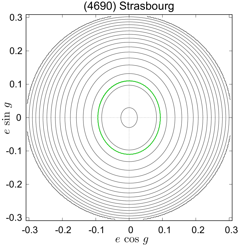
Figure 9: The motion of the asteroid (4690) Strasbourg on the $(e\cos g,e\sin g)$ plane in the CR3BP framework. The black curves are the equi-potential contours calculated from the numerical quadrature defined by Eq. (K09-53). The parameter values employed here are $(\Theta,\alpha)=(0.9045,0.3726)$. The green dots are the actual trajectories of the asteroid obtained through direct numerical integration of the equations of motion. The numerical data is identical to what was shown in the left panels of Fig. 2. The initial values of the asteroids’ orbital elements are adopted from the JPL Horizons web-interface as of June 7, 2017, and the initial location is $(e,g)=(0.1089756,105^{\circ}.515364)$.

All the asteroids’ equi-potential diagrams shown in Fig. 8 possess stationary points because their $\Theta$ values are smaller than the critical value $\left(\Theta=\frac{3}{5}\right)$ of the quadrupole level approximation. Let us bring up another example where $\Theta$ is larger. The object is the asteroid (4690) Strasbourg which we already dealt with in the left panels of Fig. 2. In Fig. 9 we plotted the equi-potential contours for this asteroid through the numerical quadrature. Then we superposed the trajectory obtained from direct numerical integration over the equi-potential contours in green. The numerical integration data are identical to what was shown in the left panels of Fig. 2. As is indicated in the caption of Fig. 9, $\Theta$ of this asteroid is as large as 0.9. With this parameter value, the asteroid’s equi-potential diagram on the $(e\cos g,e\sin g)$ plane does not possess any local extremums except for a minimum at the origin $(0,0)$. Naturally, the asteroid’s argument of perihelion $g$ just circulates quite regularly from 0 to $2\pi$.

3.8 Remarks on future prospects

In his last section “VII. Remarks,” after briefly mentioning the similarity and difference between his work and a previous work (Brouwer, 1947), Kozai makes the following comment in its second paragraph:

“The theory discussed in the present paper can be applied to the actual asteroid motion with some restrictions, as Jupiter’s eccentricity and other perturbing planets have been ignored.” (p. K598)

From the next paragraph Kozai begins stating several issues that he did not take care of in his theoretical model: (i) potential influence of Jupiter’s eccentricity $e^{\prime}$, (ii) indirect perturbation from other planets, (iii) motion of satellites around an oblate planet, and (iv) motion of satellites for which the orbital period of the Sun may not be regarded as short. We think some of his comments are suggestive, and they foresee future prospects. Let us make a brief summary of Kozai’s statements.

As for the issue (i) of non-zero $e^{\prime}$, the major part of Kozai’s statement is as follows:

“When Jupiter’s eccentricity is included, the canonical equations with two degrees of freedom must be solved, whereas $H$ is still constant and there is an energy integral. However, it may be very difficult to find any meaningful stationary solution because of an apparent rapid motion of ${g^{\prime}}^{\ast}$ due to a very small inclination. And $l+g+h$, $g+h$, and $h$ should be adopted instead of $l$, $g$, $h$. Then Jupiter’s orbit can be regarded as known, although there is no integral corresponding to $H={\rm const}$ for this case.” (p. K598)

Recalling that $H$ is one of the Delaunay elements $\bigl{(}H=L\sqrt{1-e^{2}}\cos i\bigr{)}$, the way Kozai wrote “When Jupiter’s eccentricity is included, $\ldots$ whereas $H$ is still constant,” makes us guess that he is talking about the quadrupole level approximation with “the happy coincidence” which reduces $H$ to a constant even when $e^{\prime}>0$ (see p. 2.3 of this monograph). However at the quadrupole level approximation, the doubly averaged disturbing function does not contain $g^{\prime}$. Hence we do not know what he meant by “an apparent rapid motion of ${g^{\prime}}^{\ast}$.” In addition, this description seems inconsistent with the later sentence “although there is no integral corresponding to $H={\rm const}$ for this case.” We do not exactly understand Kozai’s intention here.

As for the issue (ii) of indirect perturbation from other planets, Kozai makes a statement as follows:

“When indirect perturbations due to other planets are considered, the integral of the elimination of nodes does not hold in the form $h=h^{\prime}$. However, since Jupiter’s orbital plane deviates very little from the invariable plane, $H$ may be regarded as a stable constant, especially when the inclination of the asteroid is high.” (p. K598)

Kozai later solved the problem, and found a way to incorporate more than one perturber in this line of calculations, although their orbits must be circular.

As for the issue (iii) of the inclusion of planetary oblateness, Kozai writes as follows:

“When the motion of a satellite around an oblate planet is considered, the perturbations due to the sun and the oblateness should be taken into consideration. When the equator of the planet coincides with the ecliptic, the present theory can be applied with little modification, since both $H$ and $W^{\ast}$ are constant. However, since a term of $\cos 2g$ does not appear in the first-order disturbing function due to the oblateness, the limiting value of $H$ for the existence of a stationary solution becomes smaller or even disappears according to the ratio of the disturbing forces of the sun and the oblateness.” (p. K598)

The possibility that Kozai brought up above (the diminishing or disappearance of the limiting value of $H$ due to the planetary oblateness) is investigated in Lidov’s work as well as in some later studies. See p. 4.10 for more detail.

As for the issue (iv), Kozai did not give much description. He just stated:

“Sometimes, in the case of a satellite for which the period of one revolution of the sun may not be regarded as short, the solar mean anomaly $l^{\prime}$ may not be dropped. It is impossible, therefore, to make an exact study of a general case.” (p. K598)

Although Kozai did not bring up any actual examples, we presume that this kind of circumstance would happen when a satellite’s secular orbital variation occurs so quickly that we cannot regard the orbital period of the perturbing body (for instance, the Sun) to be negligibly short compared with the secular timescale. In this case, the double averaging procedure would be certainly inapplicable, as Kozai writes. He then continues as follows to conclude the paper:

“If, however, only the principal terms are taken in the disturbing function, stationary solutions can be derived. Lunar orbits provide us with especially interesting problem.” (p. K598)

Though Kozai’s statement may contain material directing future prospects, we do not go into its detail any further.

Later, Kozai extended his own work on this subject into various directions (e.g. Kozai, 1963c, 1969a, 1979, 1985). Also, it is worth noting that the number of asteroids whose argument of perihelion librates around $g=\pm\frac{\pi}{2}$ has significantly increased in Kozai’s publications. In Kozai (1962) it was just one: (1373) Cincinnati. In Kozai (1979) it went up to four: (944) Hidalgo, (1373) Cincinnati, (1866) Sisyphus, and (1981) Midas. In Kozai (1980) it further increased to eight (see his Table I on p. 91). Much later Kozai published a concise summary of his work on this subject (Kozai, 2004) where he reviewed the theoretical framework, not only of the doubly averaged inner CR3BP but also of the outer problem where $\alpha=\frac{a}{a^{\prime}}>1$. See Section 6.1.1 of this monograph (p. 6.1.1) for more descriptions about it.

4 The Work of Lidov

The core achievement of Kozai’s work that we browsed through in the previous section, as is summarized in Marsden (1999), is that Kozai discovered the existence of stationary points of argument of pericenter $g$ of perturbed body in the framework of the doubly averaged inner CR3BP. Kozai also quantified the condition for $g$ to be in libration around the stationary points as $\Theta<\frac{3}{5}$. Marsden begins his article with the following statement:

“The significance of Kozai’s (1962) paper lies in his showing, for the first time, that there are circumstances where the argument of pericenter in a perturbed orbit librates rather than circulates.” (p. 934)

However, nowadays it is well known that “for the first time” in Marsden’s above statement is not entirely correct—more and more people have come to know that there is a study published slightly earlier than Kozai’s work, and it deals with fundamentally the same problem (the doubly averaged inner CR3BP) and obtained fundamentally the same result as Kozai. The author of this work is Michail L’vovich Lidov (1926–1993), a scientist who worked on celestial mechanics and astronautics in the former Soviet Union. Details of his academic achievement are concisely summarized in his obituary (Lidov’s colleagues and disciples, 1994) and in many other articles (e.g. Egorov, 2001).

Before going into the details of Lidov’s work, we would like readers to be aware that there has been a rich flow of studies of the three-body problem in the Russian academic community since long before Lidov. Among these, a pair of publications (Moiseev, 1945a, b) occupies the position of a landmark. We begin this section with a brief introduction of these landmark papers. Note that there is a publication (Vashkov’yak, 2008) which serves as an excellent review of this line of studies in the former Soviet Union including Moiseev’s and Lidov’s work.

4.1 Moiseev’s work on CR3BP

Nikolay Dmitriyevich Moiseev (1902–1955) was a celestial mechanist in the former Soviet Union who produced a large number of publications on the three-body problem from the 1930s to the 1950s. Among his work, a pair of papers written in 1940 and published in 1945 about the general framework of CR3BP is still regarded as a classical standard, particularly in the field of averaged CR3BP. There is no English translation of these papers as far as we know, but the titles may be translated as “About some primary simplified schemes of celestial mechanics, obtained by means of averaging of restricted circular problem of three bodies, 1. About averaged variants of restricted circular planar problem of three bodies” (Moiseev, 1945a), and “2. About averaged variants of spatial restricted circular problem of three bodies” (Moiseev, 1945b), respectively. The section structure of the two papers is exactly the same as each other. Their only difference is that Moiseev (1945a) deals with a planar (two-dimensional) CR3BP, while Moiseev (1945b) deals with a spatial (three-dimensional) CR3BP. Let us quickly browse through the contents of these papers.

Moiseev first describes the basic equations of motion of CR3BP in Sections 1 (“Primary equations of restricted planar circular problem of three bodies” of the 1945a paper and “Primary equations of restricted spatial circular problem of three bodies” of the 1945b paper). Then in Sections 2 (“Doubly averaged Gaussian problem”) he moves on to the doubly averaged CR3BP, and illustrates the equations of motion and conserved quantities. Moiseev names this problem as the doubly averaged Gaussian problem. The differential equations for the orbital elements of the perturbed body in the spatial (three-dimensional) CR3BP that Moiseev described in Section 1 of his 1945b paper are equivalent to what we see in modern textbooks, and they are as follows:

$$\frac{da}{dt}=\frac{2\sqrt{a}}{k\sqrt{m_{\rm s}}}\frac{\partial W_{\rm j}}{\partial M},$$ (Mb1.28-101)

$$\frac{dp}{dt}=\frac{2\sqrt{p}}{k\sqrt{m_{\rm s}}}\frac{\partial W_{\rm j}}{\partial\omega},$$ (Mb1.29-102)

$$\frac{di}{dt}=\frac{\cot i}{k\sqrt{m_{\rm s}}\sqrt{p}}\frac{\partial W_{\rm j}}{\partial\omega}-\frac{1}{k\sqrt{m_{\rm s}}\sqrt{p}\sin i}\frac{\partial W_{\rm j}}{\partial\Omega},$$ (Mb1.30-103)

$$\frac{dM}{dt}=\frac{k\sqrt{m_{\rm s}}}{a\sqrt{a}}-\frac{2\sqrt{a}}{k\sqrt{m_{\rm s}}}\frac{\partial W_{\rm j}}{\partial a},$$ (Mb1.31-104)

$$\frac{d\omega}{dt}=-\frac{2\sqrt{p}}{k\sqrt{m_{\rm s}}}\frac{\partial W_{\rm j}}{\partial p}-\frac{\cot i}{k\sqrt{m_{\rm s}}\sqrt{p}}\frac{\partial W_{\rm j}}{\partial i},$$ (Mb1.32-105)

$$\frac{d\Omega}{dt}=\frac{1}{k\sqrt{m_{\rm s}}\sqrt{p\sin i}}\frac{\partial W_{\rm j}}{\partial i},$$ (Mb1.33-106)

where $m_{\rm s}$ is the central mass of the system, $k$ is used for describing the gravitational constant $\left(k^{2}={\cal G}\right)$, $\omega$ is argument of pericenter (designated as $g$ in Kozai’s work), $\Omega$ is longitude of ascending node (designated as $h$ in Kozai’s work), and $M$ is mean anomaly (designated as $l$ in Kozai’s work). Note that Moiseev uses semilatus rectum defined as

$$p=a\left(1-e^{2}\right),$$ (108)

instead of eccentricity $e$. We conjecture that Moiseev probably followed a custom to use this element in the Soviet Union academic community at that time.

$W_{\rm j}$ in Eq. (Mb1.33-106) is the disturbing function whose general form is

$$W_{\rm j}=k^{2}m_{\rm j}\left[\frac{1}{\sqrt{a_{\rm j}^{2}+{\rm R}^{2}-2a_{\rm j}{\rm R}\cos\theta}}-\frac{{\rm R}\cos\theta}{a^{2}_{\rm j}}\right],$$ (Mb1.11-108)

where ${\rm R}$ is the radial distance of the perturbed body from the central mass (designated as $r$ in Kozai’s work), $a_{\rm j}$ is the radius of the circular motion of the perturbing body (designated as $a^{\prime}$ in Kozai’s work), and $\theta$ is the angle between the positional vector of the perturbed body and that of the perturbing body (equivalent to the angle $S$ in our Fig. 1). The subscript $\mathrm{j}$ in Eq. (Mb1.11-108) implicitly means that the perturbing body that Moiseev considered is Jupiter, while the perturbed body is regarded to be an asteroid.

Moiseev states on p. 104 of his 1945b paper that, unless the distance between the perturbed and perturbing bodies becomes zero and if the distance ${\rm R}$ remains finite, $W_{\rm j}$ can be expanded into a triple Fourier series as

$$W_{\rm j}=\sum_{q=0}^{\infty}\sum_{r=-\infty}^{\infty}\sum_{s=-\infty}^{\infty}C_{qrs}(a,p,i)\cos\left(qM+r\overline{\Omega}+s\omega\right),$$ (Mb1.45-109)

where

$$\overline{\Omega}=\Omega-l_{\mathrm{j}},$$ (Mb1.39-110)

is the longitude of ascending node of the perturbed body relative to the (true) longitude of the perturbing body, $l_{\rm j}$. The conversion (Mb1.39-110) and its use in $W_{\rm j}$ practically turns the coordinate system into a rotating frame with the perturbing body (Jupiter), and eliminates the explicit time-dependence of the disturbing function $W_{\rm j}$ that is included in $l_{\mathrm{j}}$. Note that Kozai did not explicitly take care of this kind of coordinate conversion in his work.

Now in Moiseev’s Section 2, the double averaging procedure is carried out against the disturbing function $W_{\rm j}$ of Eq. (Mb1.11-108). This yields the result as follows:

$$[W_{\rm j}]=\frac{1}{4\pi^{2}}\int_{M=0}^{2\pi}\int_{l_{\mathrm{j}}=0}^{2\pi}W_{\mathrm{j}}dMdl_{\mathrm{j}}.$$ (Mb2.1-111)

From Eq. (Mb1.45-109) we know that the doubly averaged disturbing function has the general form

$$[W_{\rm j}]=\sum_{s=-\infty}^{\infty}C_{00s}(a,p,i)\cos s\omega,$$ (Mb2.5-112)

with the coefficients $C_{00s}$ as functions of $a$, $p$, and $i$. Then, the differential equations for the doubly averaged orbital elements with the doubly averaged disturbing function become:

$$\frac{da}{dt}=0,$$ (Mb2.6-113)

$$\frac{dp}{dt}=\frac{2\sqrt{p}}{k\sqrt{m_{\rm s}}}\frac{\partial[W_{\rm j}]}{\partial\omega},$$ (Mb2.7-114)

$$\frac{di}{dt}=\frac{\cot i}{k\sqrt{m_{\rm s}}\sqrt{p}}\frac{\partial[W_{\rm j}]}{\partial\omega},$$ (Mb2.8-115)

$$\frac{d\omega}{dt}=-\frac{2\sqrt{p}}{k\sqrt{m_{\rm s}}}\frac{\partial[W_{\rm j}]}{\partial p}-\frac{\cot i}{k\sqrt{m_{\rm s}}\sqrt{p}}\frac{\partial[W_{\rm j}]}{\partial i},$$ (Mb2.10-116)

$$\frac{d\Omega}{dt}=\frac{1}{k\sqrt{m_{\rm s}}\sqrt{p\sin i}}\frac{\partial[W_{\rm j}]}{\partial i}.$$ (Mb2.11-117)

Note that in the right-hand side of the equations for $\frac{d\omega}{dt}$ that was originally presented in Moiseev (1945b, Eq. (2.10) on p. 106), the negative sign at the $\frac{\partial[W_{\rm j}]}{\partial p}$ term is somehow missing. We believe it is just a typographic error, and added the negative sign in the above Eq. (Mb2.10-116).

Note also that on p. 106 of his 1945b paper, we find yet another differential equation in the same section:

$$\frac{dM}{dt}=\frac{k\sqrt{m_{\rm s}}}{a\sqrt{a}}-\frac{2\sqrt{a}}{k\sqrt{m_{\rm s}}}\frac{\partial[W_{\rm j}]}{\partial a}.$$ (Mb2.9-118)

However, we do not think this equation is practically meaningful after the averaging procedure defined as Eq. (Mb2.1-111). The averaging procedure would eliminate the mean anomaly of the perturbed body $M$ out of description of the system. So we think Eq. (Mb2.9-118) just has an implication to express the formal dependence of mean motion $(n=\frac{dM}{dt})$ of the perturbed body on the doubly averaged disturbing function and its partial derivative, $\frac{\partial[W_{\rm j}]}{\partial a}$.

The first constant of integration in this system is semimajor axis $a$, which is obtained from Eq. (Mb2.6-113). This is equivalent to the (canonically transformed) constant Delaunay element $L^{\ast}$ in Kozai’s work. Then, by dividing Eq. (Mb2.7-114) by Eq. (Mb2.8-115) Moiseev obtains

$$\frac{dp}{di}=2p\tan i,$$ (Mb2.13-118)

which can be simply integrated as

$$\int\frac{1}{2p}dp=\int\tan idi,$$ (120)

which yields

$$\ln|p|^{\frac{1}{2}}=\ln C|\cos i|^{-1},$$ (121)

with an arbitrary constant $C$. Thus we find the second constant of integration from Eq. (121) as

$$\sqrt{p}\cos i=C=\mbox{\rm constant}.$$ (Mb2.14-121)

We presume $p\geq 0$ and $0\leq i\leq\frac{\pi}{2}$. From the definition of semilatus rectum in Eq. (108), the quantity in Eq. (Mb2.14-121) turns out to be the vertical component of the angular momentum of the perturbed body. This is obviously equivalent to Kozai’s $\sqrt{\Theta}$.

The third constant of integration is the doubly averaged disturbing function $[W_{\rm j}]$ itself. We can confirm the fact that $[W_{\rm j}]$ in Eq. (Mb2.1-111) or (Mb2.5-112) is a constant by constructing the following total derivative

$$\frac{d[W_{\rm j}]}{dt}=\frac{\partial[W_{\rm j}]}{\partial p}\frac{dp}{dt}+\frac{\partial[W_{\rm j}]}{\partial i}\frac{di}{dt}+\frac{\partial[W_{\rm j}]}{\partial\omega}\frac{d\omega}{dt},$$ (123)

using the equations from Eq. (Mb2.6-113) to Eq. (Mb2.11-117). Then, let us pick the expression of $\frac{dp}{dt}$ from Eq. (Mb2.7-114), that of $\frac{di}{dt}$ from Eq. (Mb2.8-115), and that of $\frac{d\omega}{dt}$ from Eq. (Mb2.10-116). Substituting these expressions into Eq. (123), we reach the conclusion

$$\frac{d[W_{\rm j}]}{dt}=0,$$ (124)

which automatically means

$$[W_{\rm j}]={\mbox{\rm constant}}.$$ (Mb2.15-124)

Note that in this system $\frac{d[W_{\rm j}]}{dt}$ does not depend on $\Omega$. This is due to the averaging procedure (Mb2.1-111) with the relation (Mb1.39-110). As a result, the total derivative (123) does not include the term $\frac{\partial[W_{\rm j}]}{\partial\Omega}\frac{d\Omega}{dt}$.

Now we have the three constants of integration in a system with three degrees of freedom. This brings us the conclusion that the doubly averaged CR3BP is integrable by quadrature. Note that in Moiseev’s discussion it does not matter whether the system composes the inner problem or the outer one, as he did not place any specific conditions on $W_{\rm j}$ (and therefore on $[W_{\rm j}]$) except that the orbits of the perturbed and perturbing bodies do not intersect each other.

Although it is not quite relevant to the main discussion, let us incidentally mention that Moiseev also derived an expression of the Jacobi integral of the doubly averaged CR3BP in a form using orbital elements as

$$\frac{k^{2}m_{\rm s}}{2a}+k\sqrt{m_{\rm s}}n_{j}\sqrt{p}\cos i+[W_{\rm j}]={\mbox{\rm constant}}.$$ (Mb2.16-125)

A similar expression for the doubly averaged planar CR3BP is seen in his 1945a paper (Eq. (2.11) on p. 82).

Needless to say, the fact that the system is integrable does not mean that the actual procedure of quadrature is simple or easy. Moiseev just describes the formal solutions that would be calculated by quadrature as follows. The relationship (Mb2.14-121) tells us that there is a formal dependency $p=p(i)$. Also, the relationship (Mb2.15-124) tells us that there is a formal dependency $\omega=\omega(i)$. Then, by formally integrating Eq. (Mb2.8-115) we get

$$t-t_{0}=\int_{i=i_{0}}^{i}\frac{k\sqrt{m_{\rm s}}\sqrt{p}\tan i}{\frac{\partial[W_{\rm j}]}{\partial\omega}}di,$$ (Mb2.17-126)

where $i_{0}$ is the value of $i$ at $t=t_{0}$. Equation (Mb2.17-126) can be formally processed by quadrature, ending up with a function form of $i=i(t)$. We can obtain formal solutions $p(t)$, $\omega(t)$, and $\Omega(t)$ in a similar way.

The remaining part of Moiseev’s papers (his Sections 3–6) is about another class of averaging schemes, called the singly averaged problems. In the singly averaged CR3BP, the disturbing function is averaged only once either by longitude of the perturbed body or that of the perturbing body, depending on which varies faster. Sections 3 (“External variant of the singly averaged Fatou problem”) are about a variant of the singly averaging scheme called the external “Fatou” problem (Fatou, 1931). In this scheme, the disturbing function is averaged just over the longitude of the perturbing body whose orbital motion is assumed to be faster than that of the perturbed body. Therefore we deduce that the orbit of the perturbed body is located outside that of the perturbing body, hence the problem is called external. On the other hand, Sections 4 (“Internal variant of the singly averaged problem”) are about the other variant of the singly averaged CR3BP, called the internal problem. In this case the disturbing function is averaged just by longitude of the perturbed body whose orbital motion is faster than that of the perturbing body. This implies that the orbit of the perturbed body is located inside that of the perturbing body, hence the problem is called internal. The last two sections (Section 5 “Singly averaged Delaunay–Hill problem” and Section 6 “Generalized singly averaged Delaunay–Hill problem”) are about the singly averaged schemes extended to systems with a mean motion commensurability between the mean motions of the two objects using the so-called Delaunay–Hill method (cf. Grebenikov, 1970; Singh, 1977).

Although the singly averaged CR3BP may be theoretically interesting, it seems that they are not very often considered in modern celestial mechanics anymore. A possible reason is that, since the singly averaged CR3BP in three dimensions is not generally integrable, people would choose direct numerical integration rather than analytic method. This is a difference from the doubly averaged CR3BP which is principally integrable. Thus we put the singly averaged CR3BP out of the scope of this monograph. Interested readers may consult a recent study that deals with the eccentric R3BP in the singly averaged method (Domingos et al., 2013). Shevchenko (2017, Subsection 3.1, his p. 28) also has a description of the singly averaged R3BP.

4.2 Publications by Lidov

Equipped with the knowledge of the doubly averaged CR3BP in its general form that Moiseev summarized, let us move on to the introduction of Lidov’s work.

Michail L’vovich Lidov’s landmark paper (Lidov, 1961) was published in the Russian language, sixteen years after the work by Moiseev. It was soon translated into English and published in two different journals. The first one, which seems much better known than the other, is entitled “The evolution of orbits of artificial satellites of planets under the action of gravitational perturbations of external bodies,” published in Planetary and Space Science (Lidov, 1962). Compared with this, the existence of the second translation is much less known. It is entitled “Evolution of orbits of artificial satellites of planets as affected by gravitational perturbations of external bodies,” published in AIAA Journal Russian Supplement (Lidov, 1963a). See the References section of this monograph for more detailed bibliographic records of these translations. From our own personal point of view, the second translation (Lidov, 1963a) seems more accurate and closer to the original version (Lidov, 1961) than the first translation (Lidov, 1962), in terms of its English presentation as well as its choice of technical terms used in celestial mechanics. For example, the very first sentence of Lidov (1961) is translated as follows in Lidov (1962):

“Until recently, in works devoted to the evolution of the orbits of artificial satellites, investigations have been made in detail of the influence, on the orbit of the satellite, of the difference of the gravitational field of the Earth and the central and the influence of the braking of the satellite in the Earth’s atmosphere.”

while the same sentence is translated in Lidov (1963a) as:

“Until very recently, the writers of papers on the evolution of the orbits of artificial satellites studied in detail the influence exerted by the departure of the earth’s gravitational field from a central field and by atmospheric drag.”

We prefer the latter, and our summary of Lidov’s (1961) work is based on the descriptions given in Lidov (1963a). The original section titles that we sometimes refer to are also transcribed from Lidov (1963a).

Incidentally, it is interesting to note that the AIAA version of the English translation (Lidov, 1963a) has five additional paragraphs between the front matter (title and the author list) and the first paragraph of the main text (see his p. 1985). The original paper (Lidov, 1961) does not contain these, neither does the other English translation (Lidov, 1962). Judging from the contents of the additional five paragraphs, they seem to be a kind of general summary of the paper added by the translators or the reviewer of the translation. Later we briefly mention this point (p. 6.2.4 of this monograph).

Let us also note that there is a pair of subsequent publications that has a very close relationship to Lidov’s original paper. One of them (Lidov, 1963b, written in Russian) is a chapter of a proceedings volume (Subbotin et al., 1963). The other (Lidov, 1963c, written in English) is also a chapter of another proceedings volume (Roy, 1963). The contents of the two articles are almost identical to each other, and they practically serve as a supplement of Lidov (1961): Both of them contain several subjects that Lidov (1961) did not discuss, such as the equi-potential diagram for perturbed body or the effect of planetary oblateness on the motion of satellites. Hence in this monograph we essentially bunch the achievements by Lidov (1961) and Lidov (1963b, c) together, regarding them as a series of work. Section 4.10 of this monograph is a brief summary of what Lidov has further achieved in these two publications.

4.3 Lidov’s motivation and background

In the introductory part that appears before Section 1 of his paper, Lidov emphasizes the importance of including the gravitational influence of other celestial bodies than the Earth on the change of artificial satellites’ orbit. This was of less serious concern at that time, compared with the effect of the Earth’s atmospheric drag or higher-order harmonics of the Earth’s gravitational field. Lidov mentions the fact that the perigee height of an American artificial satellite (Vanguard I) exhibited a non-negligible change (Musen et al., 1960). Lidov then mentions that a Soviet Union spacecraft Luna-3 (Sedov, 1960) bound for the Moon significantly reduced its perigee height compared with its initial value after orbiting the Earth eleven times, and eventually hit the Earth’s atmosphere. Lidov also conjectures that another American orbiter, Explorer VI (Sonett et al., 1960), may have been under a similar influence of the Moon and the Sun.

Among the above-mentioned three spacecrafts, the incident concerning Luna-3 is probably the best known (e.g. Batygin, 2018). Lidov describes the incident as follows:

“In practice, the first space flight in which orbital variation was seen to be influenced to any notable degree by the gravitational attraction of the moon and the sun was that of the Soviet automatic interplanetary station (Lunik III) launched on October 4, 1959. The earth orbit into which the station transferred after approaching the moon evolved, such that in spite of the fact that the initial perigee height had been of the order of $47\times 10^{3}$ km, by the time 11 revolutions had been completed the perigee height predicted by computation was less than the radius of the earth and the station had re-entered the earth’s atmosphere.” (Lidov, 1963a, the first paragraph in the left column on p. 1986)

Note that “Lunik III” in the above is equivalent to Luna-3. This spacecraft was also known as the “automatic interplanetary station” at that time (e.g. Harvey, 2007, p. 34). There is a more detailed literal description about its orbital evolution in Sedov (1960, pp. 9–10).

After giving the historic background, Lidov states his basic assumption throughout his paper as follows:

“The basic assumption made in this paper is that there is a small enough ratio between the height of the apocenter of the satellite and the distance from the perturbing body to the central body around which the satellite is revolving. This assumption naturally restricts the class of orbits to which our formulas can be applied;” (Lidov, 1963a, the sixth paragraph in the left column on p. 1986)

We can rephrase that Lidov assumes the ratio between the orbital distance of perturbed body $r$ from the central mass and that of perturbing body $r_{k}$ is small. Although Lidov did not use any specific equations when stating this assumption, it would be expressed as follows:

$$\frac{r}{r_{k}}\ll 1.$$ (128)

As long as the eccentricity of perturbing body can be ignored, the assumption expressed by Eq. (128) is practically equivalent to $\alpha=\frac{a}{a^{\prime}}\ll 1$ that Kozai presumed. In this regard, Lidov’s discussion is limited to the quadrupole level approximation at $O\left(\alpha^{2}\right)$.

4.4 Basic equations, force components

Lidov’s Sections 1 (“Formulation of the problem and system of notation,”) and 2 (“Basic equations and perturbing forces”) are devoted to the formulation of the basic equations of motion used in his work. Unlike Kozai, Lidov did not use the Hamiltonian formalism in this study. Instead, Lidov’s work starts from the so-called Gauss’s form of equations (e.g. Brouwer and Clemence, 1961; Battin, 1987) where the time derivative of the orbital elements are expressed through three components of the perturbing force, $S$, $T$, and $W$. $S$ is the force component projected on the radius vector, $T$ is the component projected on a perpendicular direction to $S$ in the plane of the osculating ellipse, and $W$ is the component projected on a perpendicular direction to the plane of the osculating ellipse. In what follows let us transcribe the equations of motion from Lidov’s Section 2. Note that the independent variable is not the time $t$ in the following equations, but the true anomaly $\vartheta$ of the perturbed body:

$$\frac{dp}{d\vartheta} =\frac{2r^{3}\gamma}{\mu}T,$$ (L01-128)

$$\frac{de}{d\vartheta} =\frac{r^{2}\gamma}{\mu}\left[S\sin\vartheta+\left(1+\frac{r}{p}\right)T\cos\vartheta+e\frac{r}{p}T\right],$$

$$\frac{d\omega}{d\vartheta} =\frac{r^{2}\gamma}{\mu e}\left[-S\cos\vartheta+\left(1+\frac{r}{p}\right)T\sin\vartheta\right.$$

$$\left.\quad\quad\quad\quad\quad\quad\quad\quad\quad\quad-e\frac{r}{p}W\cot i\sin u\right],$$

$$\frac{d\Omega}{d\vartheta} =\frac{r^{3}\gamma}{\mu p}W\frac{\sin u}{\sin i},$$

$$\frac{di}{d\vartheta} =\frac{r^{3}\gamma}{\mu p}W\cos u,$$

where

$$\gamma=\frac{1}{1+\frac{r^{2}}{\mu e}S\cos\vartheta-\frac{r^{2}}{\mu e}\left(1+\frac{r}{p}\right)T\sin\vartheta},$$ (L02-129)

is a parameter close to 1, $u$ is argument of latitude (sum of argument of pericenter and true anomaly: $u=\omega+\vartheta$), and $\mu$ is equal to ${\cal G}\times\!$ central mass. Lidov then develops the perturbing force components $(S,T,W)$ into powers of $\frac{r}{r_{k}}$, and picks terms in the order of $\frac{r}{r_{k}}$ and $\left(\frac{r}{r_{k}}\right)^{2}$. In principle, the perturbing force $\bm{F}^{(k)}$ acting on a satellite staying at a position $\bm{r}$ from the central body under the influence of a perturbing body with a potential factor $\mu_{k}$ ($={\cal G}\times\!$ mass of the perturbing body) and a position $\bm{r}_{k}$ is expressed as

$$\bm{F}^{(k)}=\mu_{k}\left(\frac{\bm{r}_{k}-\bm{r}}{\left|\bm{r}_{k}-\bm{r}\right|^{3}}-\frac{\bm{r}_{k}}{\left|\bm{r}_{k}\right|^{3}}\right).$$ (L03-130)

Now, assume in Eq. (L03-130) that $\bm{F}^{(k)}$ can be expanded in terms of $\frac{r}{r_{k}}$ as

$$\bm{F}^{(k)}=\sum_{i=1}^{\infty}\bm{F}_{i}^{(k)}.$$ (132)

Then the first-order $(i=1)$ term of $\bm{F}^{(k)}$ becomes

$$\bm{F}_{1}^{(k)}=\frac{\mu_{k}}{r_{k}^{2}}\left[3\frac{\bm{r}_{k}}{r_{k}}\frac{\left(\bm{r}\cdot\bm{r}_{k}\right)}{r_{k}^{2}}-\frac{\bm{r}}{r_{k}}\right],$$ (L04-132)

and the second-order term becomes

$$\bm{F}_{2}^{(k)}=$$ (L05-133)

$$\;\frac{\mu_{k}}{r_{k}^{2}}\left[\left(-\frac{3}{2}\frac{r^{2}}{r_{k}^{2}}+\frac{15}{2}\frac{\left(\bm{r}\cdot\bm{r}_{k}\right)^{2}}{r_{k}^{4}}\right)\frac{\bm{r}_{k}}{r_{k}}-3\frac{\left(\bm{r}\cdot\bm{r}_{k}\right)}{r_{k}^{2}}\frac{\bm{r}}{r_{k}}\right].$$

Lidov then introduces a new coordinate system. The axis 1 of this system starts from the central mass to the pericenter of the satellite ($=$ the perturbed body), the axis 2 is orthogonal to the axis 1 and directed along the motion of the satellite and lies in the plane of the orbit, and the axis 3 is oriented normal to the plane of the satellite’s orbit. $\xi_{1}$, $\xi_{2}$, $\xi_{3}$ are the direction cosines of the position vector $\bm{r}_{k}$ in this coordinate system. Then, the force components $(S,T,W)$ in the first-order of $\frac{r}{r_{k}}$ are expressed as:

$$S_{1}^{(k)} =\frac{\mu_{k}}{r_{k}^{2}}\frac{r}{r_{k}}\left[3\xi^{2}\cos^{2}\left(\vartheta-\vartheta_{\xi}\right)-1\right],$$ (L06-134)

$$T_{1}^{(k)} =-3\frac{\mu_{k}}{r_{k}^{2}}\frac{r}{r_{k}}\xi^{2}\cos\left(\vartheta-\vartheta_{\xi}\right)\sin\left(\vartheta-\vartheta_{\xi}\right),$$

$$W_{1}^{(k)} =3\frac{\mu_{k}}{r_{k}^{2}}\frac{r}{r_{k}}\xi_{3}\xi\cos\left(\vartheta-\vartheta_{\xi}\right).$$

In the second-order they become

$$S_{2}^{(k)} =\frac{15}{2}\frac{\mu_{k}}{r_{k}^{2}}\frac{r^{2}}{r_{k}^{2}}\left[\xi^{3}\cos^{3}\left(\vartheta-\vartheta_{\xi}\right)-\frac{3}{5}\xi\cos\left(\vartheta-\vartheta_{\xi}\right)\right],$$ (L07-135)

$$T_{2}^{(k)} =-\frac{15}{2}\frac{\mu_{k}}{r_{k}^{2}}\frac{r^{2}}{r_{k}^{2}}\left[\xi^{3}\cos^{2}\left(\vartheta-\vartheta_{\xi}\right)\sin^{2}\left(\vartheta-\vartheta_{\xi}\right)\right.$$

$$\left.\quad\quad\quad\quad\quad\quad\quad\quad\quad\quad-\frac{1}{5}\xi\sin\left(\vartheta-\vartheta_{\xi}\right)\right],$$

$$W_{2}^{(k)} =\frac{15}{2}\frac{\mu_{k}}{r_{k}^{2}}\frac{r^{2}}{r_{k}^{2}}\xi_{3}\left[\xi^{2}\cos^{2}\left(\vartheta-\vartheta_{\xi}\right)-\frac{1}{5}\right],$$

where $\xi$ is defined as $\xi=\sqrt{\xi_{1}^{2}+\xi_{2}^{2}}$, and $\vartheta_{\xi}$ is the projected true anomaly of the vector $\bm{r}_{k}$ on the plane of the satellite orbit. We have the pair of relationships

$$\sin\vartheta_{\xi}=\frac{\xi_{2}}{\xi},\quad\cos\vartheta_{\xi}=\frac{\xi_{1}}{\xi}.$$ (137)

Lidov then introduces two variables as

$$\varDelta_{k}=1+e_{k}\cos\vartheta_{k},\quad\varDelta=1+e\cos\vartheta,$$ (138)

where $\vartheta_{k}$ is true anomaly of the perturbing body. Note that at this point Lidov does not assume anything about the perturbing body’s eccentricity, $e_{k}$.

Using $\varDelta_{k}$ and $\varDelta$ in Eq. (138), $r_{k}$ and $r$ are expressed as

$$r_{k}=\frac{p_{k}}{\varDelta_{k}},\quad r=\frac{p}{\varDelta},$$ (139)

with semilatus rectums $p_{k}$ and $p$. Applying Eqs. (137), (138), (139) to the expressions of $S_{1}^{(k)}$, $T_{1}^{(k)}$, $W_{1}^{(k)}$, $S_{2}^{(k)}$, $T_{2}^{(k)}$, $W_{2}^{(k)}$ in Eqs. (L06-134) and (L07-135), Lidov obtained another form of the force components as

$$S_{1}^{(k)} =3\frac{\mu_{k}}{p_{k}^{2}}\frac{p}{p_{k}}\left[\beta_{1}\cos^{2}\vartheta+2\beta_{3}\cos\vartheta\sin\vartheta\right.$$ (L08-139)

$$\left.\quad\quad\quad\quad\quad\quad\quad\quad-\frac{\beta_{6}}{3}+\beta_{2}\sin^{2}\vartheta\right]\frac{1}{\varDelta},$$

$$T_{1}^{(k)} =-3\frac{\mu_{k}}{p_{k}^{2}}\frac{p}{p_{k}}\left[\left(\beta_{1}-\beta_{2}\right)\cos\vartheta\sin\vartheta\right.$$

$$\left.\quad\quad\quad\quad\quad\quad\quad\quad+\beta_{3}\left(\sin^{2}\vartheta-\cos^{2}\vartheta\right)\right]\frac{1}{\varDelta},$$

$$W_{1}^{(k)} =3\frac{\mu_{k}}{p_{k}^{2}}\frac{p}{p_{k}}\left[\beta_{5}\cos\vartheta+\beta_{4}\sin\vartheta\right]\frac{1}{\varDelta},$$

and

$$S_{2}^{(k)} =\frac{15}{2}\frac{\mu_{k}}{p_{k}^{2}}\frac{p^{2}}{p^{2}_{k}}\left[\gamma_{1}\cos^{3}\vartheta+3\gamma_{3}\cos^{2}\vartheta\sin\vartheta\right.$$ (L09-140)

$$\left.\quad\quad\quad\quad\quad+3\gamma_{6}\cos\vartheta\sin^{2}\vartheta+\gamma_{2}\sin^{3}\vartheta\right.$$

$$\left.\quad\quad\quad\quad\quad\quad\quad-\frac{3}{5}\alpha_{1}\cos\vartheta-\frac{3}{5}\alpha_{2}\cos\vartheta\right]\frac{1}{\varDelta^{2}},$$

$$T_{2}^{(k)} =-\frac{15}{2}\frac{\mu_{k}}{p_{k}^{2}}\frac{p^{2}}{p^{2}_{k}}\left[-\gamma_{3}\cos^{3}\vartheta\right.$$

$$\left.+\left(\gamma_{1}-2\gamma_{6}\right)\cos^{2}\vartheta\sin\vartheta+\left(2\gamma_{3}-\gamma_{2}\right)\cos\vartheta\sin^{2}\vartheta\right.$$

$$\left.\quad\quad+\gamma_{6}\sin^{3}\vartheta-\frac{1}{5}\alpha_{1}\sin\vartheta+\frac{1}{5}\alpha_{2}\sin\vartheta\right]\frac{1}{\varDelta^{2}},$$

$$W_{2}^{(k)} =\frac{15}{2}\frac{\mu_{k}}{p_{k}^{2}}\frac{p^{2}}{p^{2}_{k}}\left[\gamma_{4}\cos^{2}\vartheta+2\gamma_{7}\cos\vartheta\sin\vartheta\right.$$

$$\left.\quad\quad\quad\quad\quad\quad\quad\quad+\gamma_{5}\sin^{2}\vartheta-\frac{\alpha_{3}}{5}\right]\frac{1}{\varDelta^{2}},$$

with a new set of coefficients $\alpha_{i},\beta_{i},\gamma_{i}$ which are functions of $\xi_{i}$ $(i=1\ldots)$ and $\varDelta_{k}$:

$$\alpha_{1} =\xi_{1}\varDelta_{k}^{4}, \;\;\alpha_{2} =\xi_{2}\varDelta_{k}^{4}, \;\;\alpha_{3} =\xi_{3}\varDelta_{k}^{4},$$ (L10-141)

$$\beta_{1} =\xi_{1}^{2}\varDelta_{k}^{2}, \;\;\beta_{2} =\xi_{2}^{2}\varDelta_{k}^{3}, \;\;\beta_{3} =\xi_{1}\xi_{2}\varDelta_{k}^{3},$$

$$\beta_{4} =\xi_{2}\xi_{3}\varDelta_{k}^{3}, \;\;\beta_{5} =\xi_{1}\xi_{3}\varDelta_{k}^{3}, \;\;\beta_{6} =\varDelta_{k}^{3},$$

$$\gamma_{1} =\xi_{1}^{3}\varDelta_{k}^{4}, \;\;\gamma_{2} =\xi_{2}^{3}\varDelta_{k}^{4}, \;\;\gamma_{3} =\xi_{1}^{2}\xi_{2}\varDelta_{k}^{4},$$

$$\gamma_{4} =\xi_{1}^{2}\xi_{3}\varDelta_{k}^{4}, \;\;\gamma_{5} =\xi_{2}^{2}\xi_{3}\varDelta_{k}^{4}, \;\;\gamma_{6} =\xi_{2}^{2}\xi_{1}\varDelta_{k}^{4},$$

$$\gamma_{7} =\xi_{1}\xi_{2}\xi_{3}\varDelta_{k}^{4}.$$

4.5 Three assumptions

In his Section 3 (“Basic assumptions for obtaining approximate formulas”), Lidov describes three basic assumptions that are required for deriving the averaged equations of motion in his later sections.

Assumption 1.

The first assumption is that $\gamma$ in Eq. (L02-129) is always unity. We think it is rather easy for readers to understand his intention by literally citing his words:

”It follows from Eqs. (L02) and (L06) that the maximum deviation of the value of $\gamma$ from unity is defined to the first-order by a parameter proportional to $\frac{\mu_{k}}{\mu}\left(\frac{a}{r_{k}}\right)^{3}\frac{1}{e}$ in the case of small eccentricities and by a parameter proportional to $\frac{\mu_{k}}{\mu}\left(\frac{a}{r_{k}}\right)^{3}\frac{1}{1-e}$ in the case of eccentricities close to unity (here $a$ is the semimajor axis of the orbit). For example, consider the case of perturbation by the moon of an earth satellite whose semimajor axis is of the order of 30–$40\times 10^{3}$ km. In this case

$$\frac{\mu_{k}}{\mu}\left(\frac{a}{r_{k}}\right)^{3}\sim 10^{-5}$$

This estimate shows that for a broad class of satellite orbits, with practically all values of eccentricity, we can set with a certain degree of approximation $\gamma=1$. The derivations that follow will be based on equations in which $\gamma=1$.” (Lidov, 1963a, p. 1988)

Assumption 2.

Lidov’s second assumption is quite linguistically described. Our understanding about it is as follows. The variation component of orbital elements of the satellites (such as $\Delta p$, $\Delta e$, $\cdots$) over its one revolution can be expressed in series such as

$$\Delta p=\sum_{j}\Delta_{j}p,\quad\Delta e=\sum_{j}\Delta_{j}e,\quad\cdots,$$ (143)

and their $j$-th order terms (such as $\Delta_{j}p$ or $\Delta_{j}e$ in Eq. (143)) are derived only from the $j$-th order component of the expanded perturbing force $\bm{F}_{j}$ on the right-hand side of Eq. (132). For example, $\Delta_{1}p$ is derived just from $\bm{F}_{1}$, $\Delta_{2}e$ is derived just from $\bm{F}_{2}$, and so on. Let us cite Lidov’s words concerning the second assumption:

“In the approximate treatment we have adopted, the equations describing the process become linear with a linear dependence on the perturbing forces. Thus in determining the secular change of the elements for one revolution of the satellite under the influence of a sum of accelerations $\sum_{i=1}^{n}\bm{F}_{i}$ from a wide variety of perturbing factors, we can independently determine the deviations under the influence of each of such factors, and obtain the general result by the simple summation $\Delta p=\sum\Delta p_{i}$, $\Delta e=\sum\Delta e_{i}$, $\ldots$ . In particular, we can also consider as independent the deviations of the elements under the influence of each term of series (L03) of the expansion of the perturbing acceleration in powers of $\frac{r}{r_{k}}$.” (Lidov, 1963a, p. 1988)

Assumption 3.

Lidov’s third assumption is that the coefficients $\alpha_{i},\beta_{i},\gamma_{i}$ that show up in Eq. (L10-141) can be Taylor-expanded by a small time interval $\Delta t$, and that the first two terms of the series yield approximations accurate enough for the purpose of his discussion. Let us cite Lidov’s words concerning the third assumption. In the following, $t^{\ast}$ is the time when satellite’s true anomaly satisfies $\vartheta=\pi$, i.e. the time corresponding to satellite’s position at its apocenter:

“The variability in the course of one revolution of the quantities $\alpha_{i},\beta_{i},\gamma_{i}$, determined by formulas (L10-141), with fixed orbital elements, is related to the motion of the perturbing body in absolute space.

The third important assumption we shall make in developing our approximate formulas is that the values $\alpha_{i},\beta_{i},\gamma_{i}$, can be represented in the form of the series

$$\alpha_{i} =\alpha_{i}^{\ast}+\left(\frac{d\alpha_{i}}{dt}\right)^{\ast}\Delta t+\frac{1}{2}\left(\frac{d^{2}\alpha_{i}}{dt{}^{2}}\right)^{\ast}\left(\Delta t\right)^{2}$$ (L11-143)

$$\quad\quad+\cdots$$

$$\beta_{i} =\beta_{i}^{\ast}+\left(\frac{d\beta_{i}}{dt}\right)^{\ast}\Delta t+\frac{1}{2}\left(\frac{d^{2}\beta_{i}}{dt{}^{2}}\right)^{\ast}\left(\Delta t\right)^{2}$$

$$\quad\quad+\cdots$$

$$\gamma_{i} =\gamma_{i}^{\ast}+\left(\frac{d\gamma_{i}}{dt}\right)^{\ast}\Delta t+\frac{1}{2}\left(\frac{d^{2}\gamma_{i}}{dt{}^{2}}\right)^{\ast}\left(\Delta t\right)^{2}$$

$$\quad\quad+\cdots$$

We also assume that in an interval of time equal to half the period of revolution of the satellite, with a degree of approximation adequate for study purposes, we can approximate $\alpha_{i},\beta_{i},\gamma_{i}$, by the small number of terms in the series (by two, in the present paper). Here $\Delta t=t-t^{\ast}$, where $t^{\ast}$ is a fixed instant of time interval corresponding to the given orbit.” (Lidov, 1963a, p. 1988. A more specific definition of $t^{\ast}$ shows up in p. 1989)

4.6 Averaged equations of motion

In his Section 4 (“Formulas for the variation in orbital elements for one revolution of the satellite”), Lidov carries out an averaging of the satellite’s orbital elements over its one revolution. This procedure is practically equivalent to the single averaging procedure described in Moiseev’s work. The procedure begins with substituting the expanded force components $S$, $T$, $W$ expressed as Eqs. (L08-139) and (L09-140) into the equations of motion (L01-128), and then integrating them from 0 to $2\pi$ with respect to the true anomaly of the satellite. It may sound odd for readers to hear that Lidov employed true anomaly (actually, argument of latitude) as the integration variable. However in Lidov’s averaging procedure, the actual integration procedures using the argument of latitude are ingeniously encapsulated through a Taylor-expanded conversion formula involving the true anomaly $\vartheta$ and the time increment $\Delta t$ (Eqs. (L13) and (L14), although we do not reproduce them here). We presume this conversion turns the integrations equivalent to those using mean anomaly as the integration variable. As a result, we can obtain integral formulas for the variation of the satellite’s orbital elements for its one revolution such as $\Delta_{1}^{(k)}p$ in the first-order approximation, and $\Delta_{2}^{(k)}p$ in the second-order approximation. Example expressions are shown in Lidov’s Eq. (L12) although we do not reproduce them in this monograph due to their complexity.

Next, Lidov assumes that the variations of orbital elements in each order such as $\Delta_{1}^{(k)}p$ or $\Delta_{2}^{(k)}p$ can be Taylor-expanded into a power series of the time increment, $\Delta t$. This is related to the aforementioned assumption 3 that the coefficients $\alpha_{i}$, $\beta_{i}$, $\gamma_{i}$ can be Taylor-expanded in the form of Eq. (L11-143). As a result, the variation of the satellite’s orbital element, for example $p$, is expressed as

$$\Delta_{1}^{(k)}p =\Delta_{11}^{(k)}p+\Delta_{12}^{(k)}p+\Delta_{13}^{(k)}p+\cdots,$$ (L15-144)

$$\Delta_{2}^{(k)}p =\Delta_{21}^{(k)}p+\Delta_{22}^{(k)}p+\Delta_{23}^{(k)}p+\cdots,$$

where the second terms in the right-hand sides ($\Delta_{12}^{(k)}p$ and $\Delta_{22}^{(k)}p$) correspond to the terms of $O\left(\Delta t\right)$ in Eq. (L11-143), and the third terms ($\Delta_{13}^{(k)}p$ and $\Delta_{23}^{(k)}p$) correspond to the terms of $O\left(\Delta t^{2}\right)$. Lidov shows in his Section 4 the specific forms of all the relevant terms ($\Delta_{11}a$, $\Delta_{11}e$, $\Delta_{11}i$, $\Delta_{11}\Omega$, $\Delta_{11}\omega$, $\Delta_{12}a$, $\Delta_{12}e$, $\Delta_{12}i$, $\Delta_{12}\Omega$, $\Delta_{12}\omega$, $\Delta_{21}a$, $\Delta_{21}e$, $\Delta_{21}i$, $\Delta_{21}\Omega$, $\Delta_{21}\omega$) as Eqs. (L17), (L18) and (L19), which we do not reproduce here due to their complexity. Note that the superscript $(k)$ on $\Delta_{1}^{(k)},\Delta_{12}^{(k)},\Delta_{13}^{(k)},\cdots$, denotes the influence from the $k$-th perturber. But now that Lidov considers just one perturber, the superscript $(k)$ is omitted, and $\Delta^{(k)}_{11}a$ is just written as $\Delta_{11}a$, and so forth.

At the end of his Section 4, Lidov gave several considerations on the results that he obtained in this section. The most important one we think is that both $\Delta_{11}a$ and $\Delta_{21}a$ become zero. Lidov depicts the reason as follows:

“1. The increments $\Delta_{11}a$ and $\Delta_{21}a$ are equal to zero because the increments $\Delta_{11}x$ and $\Delta_{21}x$ are for a perturbing point [that are] motionless in absolute space. For a motionless perturbing body the motion of the satellite occurs in a conservative field of force. Since it is assumed in addition that the orbital elements do not vary in the course of one revolution, then on completion of the revolution the satellite is at the same point in space and the increment of the total energy will therefore equal to zero.” (Lidov, 1963a, p. 1990. We added the content in [] for better clarity)

Although there is no mention on what $\Delta_{11}x$ and $\Delta_{21}x$ in the above quotation are in Lidov’s original description, we suspect that they are generalized symbols that denote the satellite’s orbital elements. If we generalize Eq. (L15-144) using $x$, it would become (removing all superscripts $k$):

$$\Delta_{1}x =\Delta_{11}x+\Delta_{12}x+\Delta_{13}x+\Delta_{14}x+\cdots,$$ (146)

$$\Delta_{2}x =\Delta_{21}x+\Delta_{22}x+\Delta_{23}x+\Delta_{24}x+\cdots.$$

We presume that Lidov’s above statement, particularly the “motionless” part, comes from the fact that the first terms in the right-hand side of Eq. (146) ($\Delta_{11}x$ and $\Delta_{21}x$) are in the order of $\left(\Delta t\right)^{0}=O(1)$. In other words, these quantities (belonging to the perturbing body) are $\Delta t$-independent: no matter how long or short $\Delta t$ is, these quantities would not change. Therefore, the circumstance is equivalent to having a perturbing body that is fixed in absolute space without any motion, which leads to Lidov’s above conclusion. Note that the variation components of other orbital elements such as $\Delta_{j1}p,\Delta_{j1}i,\Delta_{j1}\omega,\Delta_{j1}\Omega,\ldots$ $(j=1,2,3,\ldots)$ are not zero because of the integrated force (or moment) exerted on the satellite over its one revolution.

After some mathematical preparations in his Section 5 (“Computation of the parameters $\alpha_{i}$, $\beta_{i}$, and $\gamma_{i}$ and their derivatives for the case in which the perturbing body moves in an ellipse”) based on the assumption that the orbital motion of the perturbing body is Keplerian, Lidov extends the formulation of orbital change of the satellite over its several $(N)$ revolutions in his Section 6 (“Formulas for variation in orbital elements during several revolutions of the satellites”). The mathematical expositions in these two sections are quite detailed and lengthy. We will not go into them because they are out of the scope of this monograph. Major results exhibited in Lidov’s Section 6 are summarized in the form of finite integrals using the perturbing body’s $u$ (argument of latitude) from $u_{0}$ to $u_{N}$, corresponding to the time from $t_{0}$ to $t_{N}$, such as Eqs. (L45), (L46) and (L47).

The preparations carried out in his Sections 5 and 6 allow Lidov to move on to the next step of his approximation: deriving the secular change of the satellite’s orbital elements during one revolution of the perturbing body. This procedure is carried out in his Section 7 (“Treatment of the equations for secular variation in elements during the period of revolution of the perturbing body”). This section starts with deriving the doubly averaged equations of motion of the satellite based on the achievement obtained in the previous two sections (Sections 6 and 7). More specifically, substitution of $u_{N}=u_{0}+2\pi$ into the finite integrals calculated in Section 6, from $\int_{u_{0}}^{u_{N}}$ to $\int_{u_{0}}^{u_{0}+2\pi}$, is applied. After deriving the doubly averaged differential equations for the satellite’s orbital elements, Lidov moves on to an analysis of the characteristics of the satellite’s orbital motion. He particularly focuses on the conserved quantities of the three-body system that he considers. At this point, we finally find ourselves able to compare Lidov’s and Kozai’s results in detail.

Let us show the resulting doubly averaged differential equations of the satellite’s orbital elements in Lidov’s Section 7. He depicted them as “the equations for the variation in the orbital elements [of satellite] for one revolution, averaged for the period of revolution of the perturbing body” (Lidov, 1963a, p. 1994). Their actual forms are:

$$\frac{\delta a}{\delta N} =0,$$ (L54-146)

$$\frac{\delta e}{\delta N} =\frac{Ae\sqrt{\varepsilon}}{2}\sin^{2}i\sin 2\omega,$$

$$\frac{\delta i}{\delta N} =-\frac{A}{2}\frac{1-\varepsilon}{\sqrt{\varepsilon}}\sin i\cos i\sin 2\omega,$$

$$\frac{\delta\Omega}{\delta N} =-\frac{A\cos i}{\sqrt{\varepsilon}}\left[(1-\varepsilon)\sin^{2}\omega+\frac{\varepsilon}{5}\right],$$

$$\frac{\delta\omega}{\delta N} =\frac{A}{\sqrt{\varepsilon}}\left[\left(\cos^{2}i-\varepsilon\right)\sin^{2}\omega+\frac{2\varepsilon}{5}\right],$$

where

$$\varepsilon=1-e^{2},\quad\varepsilon_{k}=1-e_{k}^{2},\quad p_{k}=a_{k}\varepsilon_{k},$$ (148)

$$A=\frac{15\pi}{2}\frac{\mu_{k}}{\mu}\left(\frac{a}{p_{k}}\right)^{3}\varepsilon_{k}^{\frac{3}{2}}.$$ (L55-148)

Recall that $N$ denotes the number of revolutions of the satellite during one revolution of the perturbing body. The increment of the satellite’s longitude over its $N$ revolutions is $2\pi N$. It advances the satellite’s time by $2\pi N/n$ (where $n$ is the satellite’s mean motion). Therefore we see that the differentiation $\frac{\delta}{\delta N}$ in Eq. (L54-146) is directly associated with the ordinary time differentiation $\frac{d}{dt}$ as

$$\frac{\delta}{\delta N}=\frac{2\pi}{n}\frac{d}{dt}.$$ (150)

Using the relationship (150), it is straightforward to show that the differential equation for the satellite’s argument of pericenter $\omega$ (the last one in Eq. (L54-146)) is equivalent to the canonical equation of motion for $g$ at the quadrupole level (Eq. (74) on p. 3.4 of this monograph). It is also easy to construct a differential equation for $G=\sqrt{\mu a\left(1-e^{2}\right)}$ from Eq. (L54-146), and to confirm its equivalence to the canonical equation of motion, Eq. (73).

4.7 Constants of motion

Of all ten sections of Lidov’s paper in 1961, we regard Section 7 to contain the most important contents. In this section, Lidov first presents three constants of motion that the doubly averaged inner CR3BP possesses. Then he gives considerations on the solutions of the doubly averaged equations of motion (L54-146) for several special cases, based on the three constants of motion.

As Lidov writes, and as is clear from the first equation of Eq. (L54-146), the satellite’s semimajor axis $a$ is constant in his approximation. This is the first constant of motion. The second constant is what Lidov calls $c_{1}$ defined as

$$c_{1}=\left(1-e^{2}\right)\cos^{2}i,$$ (151)

or in Lidov’s original expression, it is defined as

$$\varepsilon=\frac{c_{1}}{\cos^{2}i}.$$ (L58-151)

This quantity is equivalent to Kozai’s $\Theta$ (see Eq. (K26-75) on p. K26-75 of this monograph) as well as to the square of Moiseev’s $C$ (see Eq. (Mb2.14-121) on p. Mb2.14-121 of this monograph). It is easy to confirm that $c_{1}$ is actually a constant in the framework of Lidov’s approximation as follows:

1. Differentiate $c_{1}$ of Eq. (L58-151) by the time $t$ to obtain $\frac{dc_{1}}{dt}$ .

2. Convert $\frac{\delta e}{\delta t}$ and $\frac{\delta i}{\delta t}$ into $\frac{de}{dt}$ and $\frac{di}{dt}$ using the relationship (150) .

3. Substitute $\frac{de}{dt}$ and $\frac{di}{dt}$ into $\frac{dc_{1}}{dt}$ .

And we will find $\frac{dc_{1}}{dt}=0$.

The third constant of motion, which Lidov calls $c_{2}$, makes his work unique and distinguished from other classic studies. In the work of Kozai and that of Moiseev, the third constant of motion is the doubly averaged disturbing function itself. In Kozai’s work, it is $W^{\ast}$ in Eq. (K23-70) or Eq. (72) in the quadrupole level approximation. In Moiseev’s work, it is $[W_{\rm j}]$ in Eq. (Mb2.15-124). In contrast, Lidov defines his third constant $c_{2}$ as follows:

$$c_{2}=\left(1-\varepsilon\right)\left(\frac{2}{5}-\sin^{2}i\sin^{2}\omega\right),$$ (153)

or in Lidov’s original expression, it is defined as

$$1-\varepsilon=\frac{c_{2}}{\frac{2}{5}-\sin^{2}i\sin^{2}\omega}.$$ (L59-153)

Actually, we have not found any information or descriptions as to how Lidov devised, derived, or reached the function form of Eq. (L59-153) in any of the relevant publications. An interesting point about $c_{2}$ is that, $c_{2}$ is not independent from $c_{1}$. $c_{1}$ and $c_{2}$ are connected to each other through the following relationship:

$$c_{2}=\left(1-\frac{c_{1}}{\cos^{2}i}\right)\left(\frac{2}{5}-\left(1-\frac{c_{1}}{\varepsilon}\right)\sin^{2}\omega\right).$$ (155)

Similar to the discussion about $c_{1}$, it is again straightforward to confirm that $c_{2}$ is a constant of motion in the framework of Lidov’s approximation as follows:

1. Differentiate $c_{2}$ of Eq. (L59-153) by the time $t$ to obtain $\frac{dc_{2}}{dt}$ .

2. Convert $\frac{\delta e}{\delta t}$, $\frac{\delta i}{\delta t}$, $\frac{\delta\omega}{\delta t}$ into $\frac{de}{dt}$, $\frac{di}{dt}$, $\frac{d\omega}{dt}$ using the relationship (150).

3. Substitute $\frac{de}{dt}$, $\frac{di}{dt}$, $\frac{d\omega}{dt}$ into $\frac{dc_{2}}{dt}$ .

And we will find $\frac{dc_{2}}{dt}=0$. The actual values of $c_{1}$ and $c_{2}$ are determined by the initial values of $\varepsilon$, $i$, and $\omega$ as

$$c_{1} =\varepsilon_{0}\cos^{2}i_{0},$$ (L60-155)

$$c_{2} =\left(1-\varepsilon_{0}\right)\left(\frac{2}{5}-\sin^{2}i_{0}\sin^{2}\omega_{0}\right),$$

where $\varepsilon_{0}$, $i_{0}$, $\omega_{0}$ are the initial values of $\varepsilon$, $i$, $\omega$, respectively.

After introducing $c_{1}$ and $c_{2}$, Lidov briefly mentions how to obtain a time-dependent solution for the orbital elements. Lidov states that the equations (L58-151) and (L59-153) determine the dependencies of two functions as

$$\varepsilon=f_{1}(\omega),\quad\cos i=f_{2}(\omega).$$ (157)

Note that $f_{1}$ is mistyped as $f_{i}$ in Lidov (1963a, p. 1994, below Eq. (L60)). Then Lidov expresses the solution by definite integrals, in other words, by quadrature. Literally citing his words, “the solution of the entire problem is obtained by using the two definite integrals,” (Lidov, 1963a, the right column on p. 1994). Their actual forms are as follows:

$$N-N_{0}=\frac{1}{A}\int^{\omega}_{\omega_{0}}\frac{\sqrt{\varepsilon}}{\left(\cos^{2}i-\varepsilon\right)\sin^{2}\omega+\frac{2\varepsilon}{5}}d\omega,$$ (L61-157)

$$\Omega-\Omega_{0}=-{A}\int^{N}_{N_{0}}\frac{\cos i}{\sqrt{\varepsilon}}\left[\left(1-\varepsilon\right)\sin^{2}\omega+\frac{\varepsilon}{5}\right]dN.$$ (L62-158)

The formal operation of the quadrature depicted by Eqs. (L61-157) and (L62-158) are principally equivalent to what Moiseev showed by his Eq. (Mb2.17-126) and the discussion that follows it (see p. Mb2.17-126 of this monograph).

4.8 The Lidov diagram

As is better known today, there is a major advantage to exploit $c_{2}$ as the third constant of motion of the doubly averaged inner CR3BP compared with the use of the averaged disturbing function itself. At the quadrupole level approximation, we can immediately predict if the perturbed body’s argument of pericenter librates around $\pm\frac{\pi}{2}$ or circulates from 0 to $2\pi$ just from its $c_{2}$ value without producing an equi-potential diagram. This prediction is not straightforward if we use the averaged disturbing function itself as the third constant of motion. In this subsection let us consider this issue in more detail along with Lidov’s discussion. Shevchenko (2017, his Section 3.2.3 on p. 36) also has a dedicated description for this subject.

From its definition (L58-151), $c_{1}$ takes the value from 0 to 1. From its definition (L59-153), $c_{2}$ takes the value from $-\frac{3}{5}$ to $\frac{2}{5}$. However since $c_{2}$ depends on $c_{1}$ as seen in Eq. (155), the dynamically possible area on the $(c_{1},c_{2})$ plane is not a simple rectangle, and it shapes the cyan-hatched region A–B–O–E–D–A shown in Fig. 10. The coordinates of each of the points are A$\bigl{(}1,0\bigr{)}$, B$\bigl{(}0,\frac{2}{5}\bigr{)}$, O$\bigl{(}0,0\bigr{)}$, E$\bigl{(}0,-\frac{3}{5}\bigr{)}$, and D$\bigl{(}\frac{3}{5},0\bigr{)}$. Let us call this type of plot on the $(c_{1},c_{2})$ plane as the Lidov diagram, as it first appeared in Lidov’s work.

The borders of the closed shape A–B–O–E–D–A in Fig. 10 are defined by the solutions of Eqs. (L54-146) in several special cases. The descriptions on these special cases in Lidov (1961, p. L26–L30) are quite elaborate and well organized. These solutions also help us understand the dynamical characteristics of the system described by Eq. (L54-146) in non-special, ordinary cases. We first follow Lidov’s description concerning the function form of the borders.

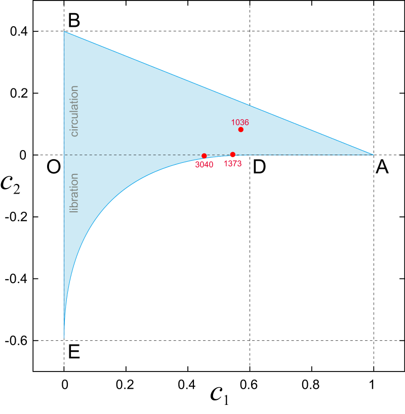
Figure 10: The Lidov diagram that indicates the possible range of $(c_{1},c_{2})$ in the doubly averaged inner CR3BP at the quadrupole level approximation. This figure is practically a reproduction of what Lidov (1961, Fig. 1 on p. L29) showed. The line $c_{2}=0$ (the line A–D–O) makes an important boundary of the perturbed body’s secular motion. When the parameter set $(c_{1},c_{2})$ of the perturbed body is above the boundary and located in the triangle $\bigtriangleup$AOB, its argument of pericenter exhibits a circulation from 0 to $2\pi$. Meanwhile it makes a libration around $+\frac{\pi}{2}$ or $-\frac{\pi}{2}$ when the parameter set $(c_{1},c_{2})$ of the perturbed body is below the boundary and located in the concave triangle $\bigtriangleup$DOE (except when it is just on the line O–D). The red dots show the locations of the parameter sets $(c_{1},c_{2})$ of the three asteroids presented in Fig. 8: (1036) Ganymed, (1373) Cincinnati, and (3040) Kozai. Their orbital elements are as of February 16, 2014, 00:00:00 CT, adopted from the JPL Horizons web-interface.

The straight line A–B

This line represents the maximum of $c_{2}$ as a function of $c_{1}$. From Eqs. (L58-151) and (L59-153), we know that $c_{2}$ takes the maximum when $\sin^{2}i=0$. This yields the maximum value of $e$ through Eq. (L58-151), and it is a constant because $c_{1}$ is constant. As a result, the line A–B indicates a planar motion ($i=0$ or $\pi$) of the perturbed body with a fixed eccentricity. From Eq. (155), we can see that $c_{2}$ and $c_{1}$ are connected to each other along this line via the following relationship:

$$c_{2}=\frac{2}{5}\left(1-c_{1}\right).$$ (160)

Note that the motion of the perturbed body along this line corresponds to what takes place at the outer boundary of the $(e\cos g,e\sin g)$ diagram that we showed in the previous section such as Fig. 8 on p. 8. It also corresponds to the lower boundaries in Kozai’s Figs. K2–K8. See Figs. 6, 7, and the discussion on p. 6 of this monograph.

The vertical straight line B–O–E

This line is realized when $c_{1}=0$. As $c_{1}$ is proportional to the perpendicular component of the angular momentum vector of the perturbed body, $c_{1}=0$ means that the motion of the perturbed body takes place on a plane orthogonal to the orbital plane of the perturbing body $(\cos i=0)$, except in the case of the very special configuration of $e=1$ which we do not consider in this monograph. Lidov gave a detailed consideration on this class of satellite orbits with $\cos i=0$ (p. L26–L28), and concluded that in most cases these orbits will turn into extremely eccentric ones until the satellite falls onto the central body within a finite length of time. Lidov (1963b, c) gave a supplemental illustration for elucidating the evolution of these type of orbits (see Section 4.10 of this monograph).

The curved line E–D

This curve represents the minimum of $c_{2}$ as a function of $c_{1}$ between $0\leq c_{1}\leq\frac{3}{5}$. From the dependency of $c_{2}$ on $c_{1}$ seen in Eq. (155), we can derive the function form of $c_{2}$ on this line through the following two steps. Lidov considers $c_{2}$ as a function of two variables, $\varepsilon$ $(=1-e^{2})$ and $\omega$. He first fixes $\varepsilon$ and searches for the value of $\omega$ that gives a local minimum of $c_{2}$. Then Lidov varies $\varepsilon$ and searches for its value that gives the minimum of $c_{2}$.

When $\varepsilon$ is fixed as a constant, we know that the lowest value of $c_{2}$ occurs when $\sin^{2}\omega=1$ from Eq. (155). In this case, Eq. (155) becomes as follows:

$$c_{2}=-\left(1-\varepsilon\right)\left(\frac{3}{5}-\frac{c_{1}}{\varepsilon}\right).$$ (161)

Then, consider $c_{2}$ in Eq. (161) as a function of $\varepsilon$, and search for its local extremums by expressing the partial derivative of $c_{2}$ with respect to $\varepsilon$ as

$$\frac{\partial c_{2}}{\partial\varepsilon}=\frac{3}{5}-\frac{c_{1}}{\varepsilon^{2}}.$$ (162)

Putting $\frac{\partial c_{2}}{\partial\varepsilon}=0$ tells us that $c_{2}$ takes a local extremum at

$$\varepsilon=\sqrt{\frac{5}{3}c_{1}}.$$ (163)

This turns out to be a minimum, because from Eq. (162) we always have

$$\frac{\partial^{2}c_{2}}{\partial\varepsilon{}^{2}}=\frac{2c_{1}}{\varepsilon^{3}}>0.$$ (164)

For $\varepsilon$ to satisfy Eq. (163), $c_{1}$ cannot be larger than $\frac{3}{5}$ because $\varepsilon$ cannot exceed 1. Substituting $\varepsilon$ of Eq. (163) into Eq. (161), we have the function form of $c_{2}$ on the curve E–D as

$$c_{2}=-\left(\sqrt{c_{1}}-\sqrt{\frac{3}{5}}\right)^{2}.$$ (165)

Having $\varepsilon$ in the form of Eq. (163) in hand, it is straightforward to confirm that $\frac{\delta\omega}{\delta N}$ in Eq. (L54-146) vanishes when initially $\sin^{2}\omega=1$. This fact means that the perturbed body’s argument of pericenter $\omega$ stays stationary at $\omega=\pm\frac{\pi}{2}$ when the system’s parameter set $(c_{1},c_{2})$ lies somewhere on the line E–D. $\frac{\delta e}{\delta N}$ also becomes zero at these points, indicating that the satellite’s eccentricity $e$ stays stationary too. From Eq. (163) or Eq. (L54-146) we have $\cos^{2}i=\frac{3}{5}\varepsilon$ in this case. As we mentioned above, the range of $c_{1}$ should be between 0 and $\frac{3}{5}$ for this case to happen. This is equivalent to the condition that Kozai gave as Eq. (78) on p. 78, $\Theta\leq\frac{3}{5}$.

In short, motion of the perturbed body on the line E–D in the Lidov diagram is equivalent to the motion at the stationary points with $g=\pm\frac{\pi}{2}$ on the $(e\cos g,e\sin g)$ plane such as Fig. 8 (p. 8 of this monograph). Since the perturbed body’s eccentricity and argument of pericenter are both constant in this case, the secular motion of its orbit would be a simple precession around the normal vector of the reference place (i.e. the perturbing body’s orbital plane). Lidov literally describes the circumstance as follows:

“4. When $\omega_{0}$ and $i_{0}$ satisfy the conditions $\cos\omega_{0}=0$ and $\cos^{2}i_{0}=\frac{3}{5}\varepsilon_{0}$ and $\varepsilon_{0}$ is arbitrary, system (L54) has a solution representing, on the average, an orbit with constant elements $\omega=\omega_{0}=\pm(\pi/2)$, $\varepsilon=\varepsilon_{0}$, $i=i_{0}=\varphi=\varphi_{0}$ where $\sin^{2}\varphi_{0}=1-\frac{3}{5}\varepsilon_{0}$. [$\cdots$] In this case the entire evolution, on the average, consists in the rotation of the orbit around a normal to the plane of the motion of the perturbing body.” (Lidov, 1963a, p. 1995, the point 4 in the right column)

The horizontal line O–D–A

This line is realized when $c_{2}=0$. From the definition of $c_{2}$ in Eq. (L59-153), we know that there can be two subcases here. It is either when

$$\sin^{2}i\sin^{2}\omega=\frac{2}{5},$$ (166)

or when

$$\varepsilon=1.$$ (167)

In the first subcase when Eq. (166) holds true, we have

$$\sin^{2}\omega=\frac{2}{5\sin^{2}i}\geq\frac{2}{5},$$ (168)

and

$$\sin^{2}i=\frac{2}{5\sin^{2}\omega}\geq\frac{2}{5}.$$ (169)

Also, by Eq. (166) $\frac{\delta\omega}{\delta N}$ in Eq. (L54-146) can be written as

$$\frac{\delta\omega}{\delta N}=A\frac{1-\varepsilon}{\sqrt{\varepsilon}}\left(\sin^{2}\omega-\frac{2}{5}\right).$$ (L73-169)

From Eq. (L73-169) and Eq. (168), we know that $\frac{\delta\omega}{\delta N}\geq 0$ is always true in this subcase.

Meanwhile from the equation of $\frac{\delta e}{\delta N}$ in Eq. (L54-146), the satellite’s $e$ would increase while $\omega<\frac{\pi}{2}$, and it would take its maximum at $\omega=\frac{\pi}{2}$. At this point, the satellite’s inclination takes its minimum value that satisfies

$$\sin^{2}i=\frac{2}{5},$$ (171)

from Eq. (169), and $\varepsilon$ also takes its minimum value as

$$\varepsilon=\frac{5}{3}\varepsilon_{0}\cos^{2}i_{0},$$ (172)

from (L58-151), where $\varepsilon_{0}$ and $i_{0}$ denote the initial values of $\varepsilon$ and $i$, respectively. The maximum value of eccentricity $e$ in this case is calculated from Eq. (172). Past this point, $e$ decreases while $\omega>\frac{\pi}{2}$, and it would gradually approach the point of $e=0$. However, since the variation rates $\frac{\delta e}{\delta N}$ in Eq. (L54-146) and $\frac{\delta\omega}{\delta N}$ in Eq. (L73-169) both become small when $e\to 0$ (or $\varepsilon\to 1$), the secular motion of the satellite in phase space near the point $e=0$ would be very slow. Formally, it takes an infinite amount of time to reach the point $e=0$.

From today’s perspective, this subcase corresponds to the motion on a separatrix that separates the motion of the satellite’s argument of pericenter into libration and circulation. Note that this subcase is realized only on the line O–D while $c_{1}\leq\frac{3}{5}$. Actually when Eq. (166) holds true, $c_{1}$ is written as

$$c_{1}=\varepsilon-\frac{2\varepsilon}{5\sin^{2}\omega}.$$ (173)

Partial derivatives of $c_{1}$ by $\varepsilon$ and by $\sin^{2}\omega$ become

$$\frac{\partial c_{1}}{\partial\varepsilon} =1-\frac{2}{5\sin^{2}\omega},$$ (174)

$$\frac{\partial c_{1}}{\partial\left(\sin^{2}\omega\right)} =\frac{2\varepsilon}{5\sin^{4}\omega}.$$

Both quantities are always greater than or equal to zero because of Eq. (168). This means that $c_{1}$ becomes its maximum when both $\varepsilon$ and $\sin^{2}\omega$ take their largest values: $\varepsilon=1$ and $\sin^{2}\omega=1$. Substituting these values into Eq. (173), we see that the maximum value of $c_{1}$ in this subcase is $\frac{3}{5}$.

On the other hand, the second subcase expressed by Eq. (167) takes place when initially $\varepsilon=1$ (or $e=0$). In this case both $\frac{\delta e}{\delta N}$ and $\frac{\delta i}{\delta N}$ in Eq. (L54-146) become zero, and the orbit of the satellite remains circular with a fixed inclination. This status can be realized anywhere on the line O–D–A, whatever value $c_{1}$ takes between 0 to 1. The motion of the satellite along this line corresponds to the origin $(0,0)$ in the $(e\cos g,e\sin g)$ diagrams such as Fig. 8 on p. 8. It also corresponds to the upper boundaries in Kozai’s Figs. K2–K8 (see our Figs. 6 and 7). Also, note that Kozai left brief descriptions on perturbed body’s motion in several cases (see Kozai’s p. K594–K595 or p. 3.5 of this monograph) which include the two subcases discussed here.

4.9 $c_{2}$ as a flag of $\omega$-libration

In the later part of his Section 7, Lidov presents a description of the satellite’s secular motion on the $(c_{1},c_{2})$ plane in more general cases, not only on the border of the hatched shape A–B–O–E–D–A of Fig. 10. Lidov explains that $c_{2}$ can be used as a flag as to whether the satellite’s argument of pericenter librates or circulates.

When $c_{2}<0$

This case is easy to understand. From the definition of $c_{2}$ in Eq. (L59-153), we have

$$\sin^{2}i\sin^{2}\omega>\frac{2}{5}.$$ (175)

Similar to the discussion when we derived Eqs. (168) and (169), the inequality (175) naturally yields

$$\sin^{2}\omega>\frac{2}{5\sin^{2}i}\geq\frac{2}{5}.$$ (176)

The inequality (176) means that $\omega$ is confined in a range centered at the position that satisfies $\sin\omega=\pm 1$ (i.e. $\omega=\pm\frac{\pi}{2}$), and it cannot complete a circulation from 0 to $2\pi$. Therefore we conclude that the motion of the satellite’s argument of pericenter $\omega$ librates when $c_{2}<0$. On the Lidov diagram (Fig. 10) this happens in the lower concave triangle $\bigtriangleup$DOE (recall that this triangle does not include the line O–D). As we mentioned before, the range of $c_{1}$ inside the triangle $\bigtriangleup$DOE is between 0 and $\frac{3}{5}$. Therefore we can state that $\omega$ exhibits libration only when both the conditions $c_{1}<\frac{3}{5}$ and $c_{2}<0$ are satisfied at the same time, as long as the quadrupole level approximation is applied.

When $c_{2}>0$

In this case we focus on the sign of $\frac{\delta\omega}{\delta N}$ in Eq. (L54-146). From the last equation of Eq. (L54-146), it is clear that the quantity

$$\left(\cos^{2}i-\varepsilon\right)\sin^{2}\omega+\frac{2\varepsilon}{5},$$ (L75-176)

is equal to $\frac{\sqrt{\varepsilon}}{A}\frac{\delta\omega}{\delta N}$, and $\frac{\sqrt{\varepsilon}}{A}$ is always positive. Hence the quantity (L75-176) determines the sign of $\frac{\delta\omega}{\delta N}$. Here Lidov introduces two subcases: when $\frac{c_{1}}{\varepsilon^{2}}\geq 1$, and when $\frac{c_{1}}{\varepsilon^{2}}<1$. The first subcase (when $\frac{c_{1}}{\varepsilon^{2}}\geq 1$) is easier to understand. From the definition of $c_{1}$ in Eq. (L58-151), the first term of Eq. (L75-176) can be rewritten as

$$\left(\cos^{2}i-\varepsilon\right)\sin^{2}\omega=\varepsilon\left(\frac{c_{1}}{\varepsilon^{2}}-1\right)\sin^{2}\omega.$$ (178)

The right-hand side of Eq. (178) is larger than, or equal to, zero if $\frac{c_{1}}{\varepsilon^{2}}\geq 1$. This means that $\frac{\delta\omega}{\delta N}\geq 0$ is always true in this subcase, and $\omega$ monotonically circulates without a libration. There is no restriction on the value of $c_{1}$ here.

In the second subcase (when $\frac{c_{1}}{\varepsilon^{2}}<1$), it is wiser to once return to the definitions of $c_{1}$ in Eq. (L58-151) and $c_{2}$ in Eq. (L59-153). Then, $\sin^{2}i$ and $\sin^{2}\omega$ can be expressed by using $c_{1}$, $c_{2}$, $\omega$ as follows:

$$\sin^{2}i =1-\frac{c_{1}}{\varepsilon},$$ (179)

$$\left(1-\cos^{2}i\right)\sin^{2}\omega =\frac{2}{5}-\frac{c_{2}}{1-\varepsilon}.$$

Substituting the expressions of $\sin^{2}i$ and $\sin^{2}\omega$ in Eq. (179) into Eq. (L75-176), Lidov found that the following inequality must hold for $\frac{\delta\omega}{\delta N}\geq 0$ to be true:

$$\frac{\frac{2}{5}-\frac{c_{2}}{1-\varepsilon}}{1-\frac{c_{1}}{\varepsilon}}\leq\frac{\frac{2}{5}}{1-\frac{c_{1}}{\varepsilon^{2}}}.$$ (L76-179)

Now that we assume $\frac{c_{1}}{\varepsilon^{2}}<1$, and $0\leq\varepsilon\leq 1$ by the definition of $\varepsilon$, we have the following relationship:

$$1-\frac{c_{1}}{\varepsilon}\geq 1-\frac{c_{1}}{\varepsilon^{2}}>0.$$ (181)

From Eq. (181), we see that the inequality (L76-179) holds always true as long as $c_{2}>0$. This means that, in this subcase too, $\frac{\delta\omega}{\delta N}\geq 0$ is true regardless of the value of $c_{1}$. Thus $\omega$ monotonically circulates without libration when $c_{2}>0$.

By now, we see that it is proven that the satellite’s argument of pericenter $\omega$ librates when $c_{2}<0$ and $c_{1}<\frac{3}{5}$, while it circulates when $c_{2}>0$. $c_{2}=0$ is a special case that happens exactly on the line O–D–A in the Lidov diagram, as we have already seen. We might want to say that $\omega$ still librates on the separatrix that overlaps with the line O–D.

The following explains how to utilize the Lidov diagram. In Fig. 10, we plotted the actual parameter values $(c_{1},c_{2})$ of the three asteroids as a set of examples whose trajectories we integrated in Fig. 8: (1373) Cincinnati, (1036) Ganymed, and (3040) Kozai. The locations of their $(c_{1},c_{2})$ are designated by the red points in Fig. 10. We see that Ganymed is clearly located inside the triangle $\bigtriangleup$AOB, indicating that this asteroid’s argument of pericenter circulates. It is consistent with the numerical results presented in Fig. 8. On the other hand, Cincinnati and Kozai are located inside the concave triangle $\bigtriangleup$DOE (although they are very close to the boundary O–D–A). This indicates that arguments of pericenter of these asteroids librate around $\omega=\frac{\pi}{2}$ or $-\frac{\pi}{2}$. As we saw, this is exemplified by the numerical results presented in Fig. 8 where we see $\omega$ of Cincinnati librates around $\omega=\frac{\pi}{2}$, and that of Kozai librates around $\omega=\frac{3\pi}{2}$.

Here let us note two things. First, the parameter values of $(c_{1},c_{2})$ of the three asteroids plotted in Fig. 10 may not be perfectly precise. The hatched shape in Fig. 10 was drawn from the doubly averaged disturbing function. Meanwhile, the location of the red points of the actual asteroids were calculated using their osculating, non-averaged orbital elements taken from the JPL Horizons web-interface. The short-term oscillation of the asteroids’ osculating elements blurs the location of their $(c_{1},c_{2})$ in general. Second, even if we use averaged orbital elements of the asteroids for locating their $(c_{1},c_{2})$ combinations, we should be aware that the borders $c_{2}\lessgtr 0$ may not rigidly work out for distinguishing their motion between libration and circulation. This is because the Lidov diagram of Fig. 10 is produced based on the quadrupole level approximation. It uses the truncated doubly averaged disturbing function at $O\left(\alpha^{2}\right)$. Actually, $\alpha^{2}$ of the three asteroids with respect to Jupiter is not negligibly small. Specifically, $\alpha^{2}\sim 0.13$ for (3040) Kozai, $\alpha^{2}\sim 0.26$ for (1036) Ganymed, and $\alpha^{2}\sim 0.43$ for (1373) Cincinnati. Therefore their secular motion may not be well represented by the quadrupole level approximation.

In the remaining part of his Section 7, Lidov calculates the maximum and minimum values of $\varepsilon$ and their dependence on $c_{1}$ and $c_{2}$ when $c_{2}>0$ (Eqs. (L77)–(L80), although we do not reproduce them here). In this case the maximum of $\varepsilon$ (and the minimum of $e$) occurs when $\omega=0$ or $\pi$, and the minimum of $\varepsilon$ (and the maximum of $e$) occurs when $\omega=\pm\frac{\pi}{2}$. Lidov also presented similar equations for the case of $c_{2}<0$ (Eqs. (L82)–(L85), not reproduced here). The end part of Section 7 is devoted to presenting several plots of extreme values of the satellite’s eccentricities and arguments of pericenter as $c_{1}$ and $c_{2}$ being parameters (Figs. L2, L3, L4 on pp. L32–L33, not reproduced here).

Lidov’s last three sections are as follows: Section 8 “Estimates of oscillations in the pericenter height of a satellite orbit during the period of revolution of the perturbed body, Section 9 “Method of computing the revolution of the orbit of an artificial Earth satellite using approximate formulas, and Section 10 “Comparison of the results of computation by approximate formulas with the precise solution of the problem by numerical integration of the differential equations. They are largely devoted to descriptions of the practical computation method of the satellite’s orbital evolution, as well as a comparison of the results from Lidov’s analytic approximation and that of the direct numerical integration of the equations of motion. Although these sections probably had practical importance in satellite dynamics at that time, nowadays we think that most of these sections can be replaced for more efficient numerical procedures. Therefore we do not deal with these sections in this monograph.

4.10 Newly added issues in Lidov (1963b, c)

At the end of this section, let us mention a few issues that show up only in Lidov’s supplementary publications (Lidov, 1963b, c), and not in his main paper in 1961.

One of them is the treatment of a special case when the orbital inclination $i$ of the perturbed body (satellite) is just $90^{\circ}$ (Lidov, 1963c, p. 174). This corresponds to the motion that happens on the line B–O–E of the Lidov diagram (Fig. 10). For this case, Lidov gave a detailed illustration as to the dependence of the motion of argument of pericenter $\omega$ of the perturbed body on its initial value, $\omega_{0}$. He even gave an analytic solution that represents the time evolution of $\omega$ using an elliptic integral of the first kind (Lidov, 1963c, Eq. (15) and a table on p. 175). As an actual example, Lidov succeeded in obtaining a quantitative estimate that an Earth-orbiting satellite whose semimajor axis and eccentricity are the same as those of the Moon and whose inclination with respect to the ecliptic is $90^{\circ}$, can fall back to the surface of the Earth within $\sim$52 revolutions ($\sim$4 years). Lidov also carried out the numerical integration of the equations of motion of the satellite. He did a similar calculation using the singly averaged approximation. Both calculations demonstrate how quickly the minimum distance from the satellite to the Earth’s surface becomes reduced (Lidov, 1963c, Fig. 7 on p. 178). His numerical result (54 or 55 revolutions until the fall of the satellite) agrees well with his analytic estimate ($\sim$52 revolutions). This anecdote is cited by Beletsky (1972, see p. 95–100 of its English translation, ()), by Vashkov’yak (2008, his p. 9–10), and by Shevchenko (2017, his p. 7–8) with a famous cartoon where a man (a caricature of Lidov) is about to release the Moon on the $i=90^{\circ}$ orbit around the Earth.

Another subject that Lidov (1963b, c) newly added is the treatment of oblateness of the central mass (Lidov, 1963c, Section “3. The influence of the noncentricity of the gravitational field,” p. 176–177). The set of equations of motion that Lidov introduced includes the effect of oblateness of the central body through parameters $\delta$ and $\beta$ (Lidov, 1963c, Eqs. (1) and (2) on p. 169). As a consequence, although no detail is given, Lidov claimed that he found that the existence or non-existence of stationary points of perturbed body’s argument of pericenter $\omega$ depends on $\beta$, i.e. on the oblateness of the central body. He concluded that the stationary points of $\omega$ happen only when the effect of oblateness is weak. Readers must remember that Kozai also mentioned this point (see p. 3.8 of this monograph) but without showing anything specific or quantitative. However, we do not know how Lidov derived the terms that represent the oblateness of the central body appearing in his equations of motion, because Lidov did not give any details about the derivation.

5 The Work of von Zeipel

Edvard Hugo von Zeipel (1873–1959) was a Swedish scientist in astronomy and mathematics. As is mentioned in his biographical sketches such as Solc (2014), von Zeipel is famous for his pioneering achievements in many fields of theoretical astronomy, in particular, for his early work on the singularities of the $N$-body problem (von Zeipel, 1908). Diacu and Holmes (1996) made a brief but excellent review of his achievement on this subject. von Zeipel’s name is also embedded in a theorem called the von Zeipel theorem related to his later work on the calculation of radiative equilibrium of a rotating star (e.g. von Zeipel, 1924a, b, c). Nowadays, we are probably aware of his name most often in celestial mechanics, particularly related to perturbation theories: von Zeipel constructed a canonical perturbation method (von Zeipel, 1916a, b, 1917a, 1917b) which is now called the von Zeipel method. In this series of work, he devised a method for introducing generating functions to carry out canonical transformations proposed by Delaunay (1860, 1867) in order to systematically reduce the degrees of freedom of systems by the averaging procedure (for more detail, see Brouwer and Clemence, 1961; Meffroy, 1966; Boccaletti and Pucacco, 1998). These works are fundamental milestones in modern celestial mechanics, followed by numerous confirmations and extensions (e.g. Brown and Shook, 1933; Hori, 1966, 1967; Musen, 1968; Deprit, 1969; Yuasa, 1971).

von Zeipel’s work on perturbation theory in celestial mechanics is very popular, and its reputation is well established. However it is almost not known at all that, while making the epoch-making achievements mentioned above, von Zeipel also worked on a theoretical subject that is equivalent to what we have already discussed in this monograph—the doubly averaged CR3BP, in particular when inclination of the perturbed body is large. In this section we will summarize the major contents of one of von Zeipel’s publications about this subject. Our aim is to show that the basic theoretical structure of the Lidov–Kozai oscillation was already established in the early twentieth century almost at the same depth or deeper. The publication that we are going to focus on from now is von Zeipel (1910), entitled “Sur l’application des séries de M. Lindstedt à l’étude du mouvement des comètes périodiques,“ written in French and published in Astronomische Nachrichten. The full text of this paper is available on ADS. As far as we know from the records on ADS and on Web of Science (hereafter referred to as WoS), this paper has been cited only once in a modern science context, only by Bailey and Emel’yanenko (1996, through which we learned of the existence of ’s contribution).

Note that as far as we can ascertain, von Zeipel did not mention his first name (Edvard) at all in any of his own publications. We follow his way and refer to him as Hugo von Zeipel in the title of this monograph. Note also that his name is sometimes mentioned and cited just as Zeipel (e.g. Merman, 1982; Orlov, 1965b; Bailey and Emel’yanenko, 1996). But we call him von Zeipel throughout the monograph. See Supplementary Information 4 for a more detailed discussion and consideration on this subject.

5.1 Purpose, method, findings

As is obvious from its title (which can be translated into English as “On the application of the Lindstedt series to study the motion of periodic comets”), von Zeipel’s major objective in this publication is to establish a mathematical representation of the motion of periodic comets as precisely as possible using a method called the Lindstedt series. von Zeipel’s interests particularly lies in the orbital variation of comets that have a large orbital inclination. The beginning part of the paper entitled “Introduction” (pp. Z345–Z347, before his Chapter I begins) well summarizes von Zeipel’s purpose, method, and important findings. For facilitating an understanding of von Zeipel’s intentions, we believe that literally citing several paragraphs from the “Introduction” is appropriate. Note that the English translation from French appearing in what follows are all due to the present authors of this monograph. We have added several expressions in $[\;]$ for supplementing an understanding of the translation.

At the beginning, von Zeipel states the standard method for constructing analytic solutions of planetary motion at his time and its limitation:

“It is well known that in calculating the motion of planets, some series, called by Mr. Poincaré, the Lindstedt series, can be used. Elements of the planets are thus developed in powers of a small quantity $\mu$ of the order of planetary masses. The coefficients of the various powers of $\mu$ are Fourier series of a number of linearly dependent arguments of time. In the series, it is essentially assumed that the masses of the planets are relatively small compared with that of the Sun. But in the applications made so far, it was also recognized that eccentricities and inclinations of the orbits are small.” (p. Z345)

Let us just say at this point that calculating the Lindstedt series is a way of constructing approximate periodic solutions. We will see more detail about this in Section 5.3.

There, von Zeipel mentions the difficulty of constructing general theories of planetary orbital motion when their eccentricity $e$ and inclination $I$ are arbitrary:

“Trying to study, by means of series that analogues the motion of a planetary system, when eccentricities and inclinations are arbitrary, we face the difficulty in solving the equations of secular variations in a general way.” (p. Z345)

Next, von Zeipel states a possible direction for solving this problem. In what follows $R$ denotes the secular part of the disturbing function. He claims that he shows a possibility of constructing the Lindstedt series around $R$’s local extremums, not just around $R$’s minimum at $e=0$ and $I=0$ when an object’s $e$ and $I$ are as small as the major planets, but at other places in phase space even when object’s $e$ or $I$ is not small. Here is von Zeipel’s statement:

“We know that the function $R$ is minimum when the eccentricities and inclinations becomes zero. Because of this property of the function $R$, it is possible to form the series of Lindstedt representing the motion of the planets, whose eccentricities and inclinations are small. But, the function $R$ often owns other maxima and minima. When the value of $R$ is close to such a maximum or minimum value, it is still possible to calculate the Lindstedt series representing the motion. In the orbits thus obtained, the eccentricities and inclinations can be considerable. This is what I propose to show in this memoire.” (p. Z345)

Now, von Zeipel describes the dynamical model that he employs in this study—CR3BP. He also mentions the integrability of the secular version of this problem:

“In order not to complicate the exposition, I will confine myself first to a special case assuming that an infinitely small mass (asteroid, comet, meteorite or satellite) is attracted to the Sun and a perturbing planet moving around the Sun in a circle. In the study of the motion of such a body, it shall be reduced to a system of canonical differential equations with three degrees of freedom, and falling within the general type of equations, which has been studied by Mr. Poincaré in his work $\gg$Les Méthodes Nouvelles de la Mécanique Céleste$\ll$, vol. II, Chapter XI. The equations of secular variations form a canonical system, whose degree of freedom is unity. They can therefore be integrated by a quadrature and by trigonometric series of a single argument.” (pp. Z345–Z346)

However, as we are already aware, formal integrability of the doubly averaged CR3BP does not mean that we can immediately obtain actual time-dependent solutions with explicit function forms. von Zeipel mentions this point, and claims that in this study he limits himself to only finding approximate solutions around the local extremums of $R$:

“But, although the existence of these series is demonstrated, we do not know in general how to form their coefficients analytically. Thus, trying to calculate the Lindstedt series, we are forced, even in this relatively simple case, to limit the problem and assume that we are in the vicinity of a maximum or minimum value of the secular part of the disturbing function.” (p. Z346)

After briefly mentioning the contents of his Chapters II and III, von Zeipel describes the contents of his Chapter IV that contains the most important aspects of his study. It begins with the following sentence:

“Research on the maxima and minima of the secular part of the disturbing function, described in Chapter IV, shows that orbits with large inclinations and always having small eccentricities can exist only outside the disturbing planet.” (p. Z346)

We find this statement true if we remember the studies by Lidov and Kozai. When the inclination of the perturbed body is larger than a certain value ($i_{0}$ in Kozai’s work), stationary points of the argument of pericenter appear with separatrix. In this case, the eccentricity of the perturbed bodies cannot always stay small (see Fig. 8a on p. 8 of this monograph). Therefore it is concluded that, for the perturbed body to always have both a large inclination and a small eccentricity, it cannot be in an inner CR3BP system. In other words, von Zeipel’s statement above depicts the circumstance that the outer CR3BP realizes. We will later return to this point in Section 5.7 of this monograph.

Immediately after the above sentence, von Zeipel continues his statement as follows. We are certain that readers of this monograph will notice the equivalence of this statement to what was obtained by Lidov and Kozai:

“At inside the orbit of this planet, there can be asteroids with inclinations exceeding a certain limit, depending on the ratio $\alpha$ of the two major axes. This limit is about $39^{\circ}$ from the Sun, and it decreases when $\alpha$ increases, and it vanishes when $\alpha=1$. For orbits with large inclinations and inside the disturbing planet, the upper limit of the eccentricity is considerable—even if the lower limit is small—and it [the upper limit] approaches unity when the inclination is close to $90^{\circ}$. Such an orbit will be, under certain conditions, disrupted by the disturbing planet.” (p. Z346)

The above phrase “about $39^{\circ}$” must ring a bell with readers, because it is equivalent to the limiting inclination that Lidov and Kozai discussed: $\cos^{-1}\sqrt{\frac{3}{5}}\sim 39^{\circ}.23$.

Then, von Zeipel moves on to stating his findings about a categorization of stable cometary orbits along with the motion of their argument of perihelion $g$. Note that his following statement depicts three patterns of $g$’s motion: Libration around $\pm\frac{\pi}{2}$, libration around $0$ or $\pi$, and circulation from $0$ to $2\pi$. This means that his statement is not only about the inner CR3BP but also about the outer CR3BP, and also about the systems with orbit intersection:

“The studies mentioned in Chapter IV also helped me establish that there can be orbits of comets in stable motion, dependent on 6 arbitrary constants of integration. $[\ldots]$ As for the distance $g$ from the perihelion to the node, there is a first type of comets in stable motion, for which $g$ is always close to $\pm 90^{\circ}$, a second type, where $g$ is always close to $0^{\circ}$ or $180^{\circ}$, and finally a third type, where this angle $g$ is driven by a mean motion.” (pp. Z346–Z347)

von Zeipel also mentions the possible extension of his theory to more general systems that contain more than one perturbers whose orbits are nearly circular and planar:

“The results, which we have arrived [at] in the simple case, where there is only one disturbing planet, are also valid in the more general case, where an infinitely small mass is attracted to the Sun and a number of planets, whose masses, eccentricities and inclinations are small.” (p. Z347)

von Zeipel states the following theorem at the end of his “Introduction.” Here he mentions the dependence of the limiting inclination on the ratio of the semimajor axes, $\alpha$:

“The study of secular perturbations in this general case leads us to the following theorem:

For the eccentricity of the orbit of the infinitely small mass, being small at some point, is still small, it is necessary and sufficient that the inclination is situated within certain limits, which are functions of the planetary masses and the ratio of the major axes.

A slight resistance against the motion, which has the effect of reducing the major axis and eccentricity, also tends to establish limits for the inclination. ” (p. Z347)

5.2 Equations of motion of perturbed body

Following the Introduction, von Zeipel presents four major chapters (Chapters I, II, III, IV) and a short, additional chapter at its end (Chapter V). From the viewpoint of comparison between von Zeipel’s work and Lidov’s or Kozai’s work, we would say that the most important aspects of von Zeipel’s work are in its Chapter IV where he searches local extremums of the doubly averaged disturbing function of CR3BP with specific forms. Other chapters do not particularly deal with the disturbing function with specific forms. von Zeipel’s Chapter I is placed for describing the general equations of motion for CR3BP. In Chapter II von Zeipel develops general framework to apply the Lindstedt series to the disturbing function. Chapter III serves as a general study of the secular part of the CR3BP disturbing function including the case of orbit intersection. In what follows we summarize von Zeipel’s Chapter I in our Section 5.2, Chapter II in Sections 5.3 and 5.4, Chapter III in Section 5.5, Chapter IV in Sections 5.6, 5.7, 5.8, and Chapter V in Section 5.9.

von Zeipel’s first chapter “Chapitre I. Equations différentielles du mouvement,” contains four sections (Z1–Z4). This chapter is devoted to describing the equations of motion of the perturbed body in CR3BP using the Hamiltonian formalism. von Zeipel first describes the canonical equations of motion using the ordinary Delaunay elements. Then he introduces another set of equations of motion using a set of Poincaré-like canonical variables. At this point, no averaging is applied to any variables or equations.

Throughout his paper, the unit of length that von Zeipel uses is the constant distance between Jupiter and the Sun. The unit of mass is the total mass of Jupiter and the Sun. The unit of time is defined so that the Gauss constant becomes 1. In what follows, $\mu$ denotes the mass of Jupiter, and $H$ appearing in the disturbing function designates the angle between the radius vectors of the perturbed body and that of the perturbing body at the Sun (equivalent to the angle $S$ in our Fig. 1). The resulting equations of motion are:

$$\frac{dx}{dt} =-\frac{\partial\Phi}{\partial x^{\prime}}, \;\;\;\;\frac{dx^{\prime}}{dt} =\frac{\partial\Phi}{\partial x},$$ (Z01-181)

$$\frac{dy}{dt} =-\frac{\partial\Phi}{\partial y^{\prime}}, \;\;\;\;\frac{dy^{\prime}}{dt} =\frac{\partial\Phi}{\partial y},$$

$$\frac{dz}{dt} =-\frac{\partial\Phi}{\partial z^{\prime}}, \;\;\;\;\frac{dz^{\prime}}{dt} =\frac{\partial\Phi}{\partial z},$$

with

$$\Phi =-\frac{1}{2}\left({x^{\prime}}^{2}+{y^{\prime}}^{2}+{z^{\prime}}^{2}\right)+\frac{1}{r}$$ (183)

$$\quad+\mu\left(\frac{1}{\sqrt{1-2r\cos H+r^{2}}}-r\cos H-\frac{1}{r}\right),$$

where $x,y,z$ are the coordinates of the perturbed body, $x^{\prime},y^{\prime},z^{\prime}$ are their time derivatives (i.e. velocity), and $r$ is the radial distance of the perturbed body from the Sun.

Readers may find it slightly odd here to find a second term $\left(+\frac{1}{r}\right)$ and the last one in the parentheses of the third term $\left(-\frac{1}{r}\times\mu\right)$ in Eq. (183). Indeed from these two terms, we can make up a new term $\frac{1-\mu}{r}$. By the definition of the unit of mass, $1-\mu$ is the Sun’s mass. This new term can be considered as a potential that drives the Keplerian motion of the perturbed body around the Sun. However, the time average of $\frac{1}{r}$ becomes $\left<\frac{1}{r}\right>=\frac{1}{a}$, which is a constant in the doubly averaged CR3BP. Therefore, the terms proportional to $\frac{1}{r}$ in Eq. (183) merely serve as additional constants, and they have no influence on the following discussions.

Next, von Zeipel introduces a set of canonical equations of motion of the perturbed body using the Delaunay elements $L,G,\Theta,l,g,\theta$. Note that von Zeipel uses a variable $\theta$ for longitude of ascending node, instead of the modern standard notation, $h$. He also uses a variable $\Theta$ instead of the conventional notation, $H$. The equations are:

$$\frac{dL}{dt} =+\frac{\partial\Phi}{\partial l}, \;\;\;\;\frac{dl}{dt} =-\frac{\partial\Phi}{\partial L},$$ (Z02-183)

$$\frac{dG}{dt} =+\frac{\partial\Phi}{\partial g}, \;\;\;\;\frac{dg}{dt} =-\frac{\partial\Phi}{\partial G},$$

$$\frac{d\Theta}{dt} =+\frac{\partial\Phi}{\partial\theta}, \;\;\;\;\frac{d\theta}{dt} =-\frac{\partial\Phi}{\partial\Theta},$$

where

$$\Phi =\Phi_{0}+\mu\Phi_{1},$$ (185)

$$\Phi_{0} =\frac{1}{2L^{2}},$$ (186)

$$\Phi_{1} =\frac{1}{\Delta}-r\cos H-\frac{1}{r}.$$ (187)

Definition of $\Delta$ in Eq. (187) somehow does not show up in this section (it shows up much later in Section Z13 in Chapter III, p. Z368). But we see $\Delta$’s specific form in the third term in Eq. (183): it is the distance between the perturbing body and the perturbed body as follows:

$$\Delta=\sqrt{1-2r\cos H+r^{2}}.$$ (188)

Since the length of the positional vector of the perturbing body $(r^{\prime})$ is fixed to unity in von Zeipel’s work, $\Delta$ in Eq. (188) looks slightly different from what we usually see in the modern literature. von Zeipel’s unit definition $(a^{\prime}=1)$ thus sometimes causes confusion. We may rather want to understand that quantities concerning length are implicitly normalized by Jupiter’s semimajor axis in von Zeipel’s descriptions, such as $a=\frac{a}{a^{\prime}}$ or $r=\frac{r}{a^{\prime}}$.

Then, von Zeipel points out that the longitude of the perturbing body is expressed as $\pm t$ in this system, as is obvious from his definition of units. Here $+t$ corresponds to the prograde orbital motion of the perturbing planet, and $-t$ corresponds to the retrograde orbital motion. As is well known, the disturbing function of this kind of system contains $\pm t$ (for the perturbing body) and $\theta$ (for the perturbed body) only as the combination of $\theta-(\pm t)=\theta\mp t$ (e.g. Brouwer and Clemence, 1961; Nakai and Kinoshita, 1985). Therefore von Zeipel defines a new variable $\theta^{\prime}=\theta\mp t$ instead of $\theta$, and brings it into the equations of motion. Let us cite von Zeipel’s original description:

“The angle $\theta$ and the longitude of the disturbing planet are reckoned on the plane of the orbit of this planet in a sense that, at the nodes, [they] make the acute angle $I$ with the direction of angles $l$ and $g$. The longitude of the disturbing planet is represented by $\pm t$, following whether this planet orbits in the direct way or in the indirect way.

That being so, it is obvious that the disturbing function contains two longitudes $\theta$ and $t$ in combination of $\theta\mp t$. We consequently assume

$$\theta^{\prime}=\theta\mp t.$$

Equations (Z02) still survives if we write $\theta^{\prime}$ and $\Phi\pm\Theta$ instead of $\theta$ and $\Theta$.” (pp. Z348–Z349)

From the modern viewpoint, the conversion from $\theta$ to $\theta^{\prime}$ is equivalent to a coordinate conversion of the inertial frame into the rotating frame of the perturber’s orbital motion (e.g. Szebehely, 1967). This conversion generates an additional term in the Hamiltonian of the system (such as $\pm x_{2}$ in $F_{0}$ in Eq. (193)). However, terms of this kind would not affect the secular motion of the perturbed body at all.

Next in Section Z2, von Zeipel introduces another series of canonical equations of motion using a new set of canonical variables $(x_{1},x_{2},x_{3},y_{1},y_{2},y_{3})$ that are a combination of the conventional Delaunay elements as:

$$x_{1} =L, \;\;\;\;x_{2} =\Theta, \;\;\;\;x_{3} =L-G,$$ (189)

$$y_{1} =l+g, \;\;\;\;y_{2} =\theta^{\prime}, \;\;\;\;y_{3} =-g,$$

together with

$$\xi=\sqrt{2x_{3}}\cos y_{3},\quad\eta=\sqrt{2x_{3}}\sin y_{3}.$$ (190)

The variables in Eq. (189) and Eq. (190) satisfy the following canonical equations of motion:

$$\frac{dx_{\nu}}{dt} =\frac{\partial F}{\partial y_{\nu}}, \;\;\;\;\frac{dy_{\nu}}{dt} =-\frac{\partial F}{\partial x_{\nu}},$$ (Z03-190)

$$\frac{d\xi}{dt} =\frac{\partial F}{\partial\eta}, \;\;\;\;\frac{d\eta}{dt} =-\frac{\partial F}{\partial\xi},$$

where $\nu=1,2$ with

$$F =F_{0}+\mu F_{1},$$ (192)

$$F_{0} =\frac{1}{2x_{1}^{2}}\pm x_{2},$$ (193)

$$F_{1} =\frac{1}{\Delta}-r\cos H-\frac{1}{r}.$$ (194)

He then states that the perturbation Hamiltonian $F_{1}$ in Eq. (194) can be formally expanded in a Fourier series as

$$F_{1} =\sum C_{m_{1},m_{2}}\left(\xi,\eta\right)\cos\left(m_{1}y_{1}+m_{2}y_{2}\right)$$ (Z04-194)

$$+\sum S_{m_{1},m_{2}}\left(\xi,\eta\right)\sin\left(m_{1}y_{1}+m_{2}y_{2}\right).$$

Note that the coefficients $C_{m_{1},m_{2}}$ and $S_{m_{1},m_{2}}$ depend also on the variables $x_{1}$ and $x_{2}$.

In Section Z3, von Zeipel introduces yet another set of canonical variables $\left(x^{\prime}_{1},x^{\prime}_{2},x^{\prime}_{3},y^{\prime}_{1},y^{\prime}_{2},y^{\prime}_{3}\right)$ as

$$x^{\prime}_{1} =L, \;\;x^{\prime}_{2} =L-\Theta, \;\;x^{\prime}_{3} =G-\Theta,$$ (196)

$$y^{\prime}_{1} =l+g+\theta^{\prime}, \;\;y^{\prime}_{2} =-g-\theta^{\prime}, \;\;y^{\prime}_{3} =g,$$

together with

$$\xi^{\prime}=\sqrt{2x^{\prime}_{3}}\cos y^{\prime}_{3},\quad\eta^{\prime}=\sqrt{2x^{\prime}_{3}}\sin y^{\prime}_{3},$$ (197)

and a relationship that shows their canonical equivalence

$$x^{\prime}_{1}y^{\prime}_{1}+x^{\prime}_{2}y^{\prime}_{2}+x^{\prime}_{3}y^{\prime}_{3}=Ll+Gg+\Theta\theta^{\prime}.$$ (198)

The variables in Eqs. (196) and (197) may come in handy when the orbital inclination of the perturbed body is small. von Zeipel later uses them in his Section Z25, Chapter IV, p. Z413 (see also p. 5.9.1 of this monograph). The variables $x^{\prime}_{1}$, $x^{\prime}_{2}$, $y^{\prime}_{1}$, $y^{\prime}_{2}$, $\xi^{\prime}$, $\eta^{\prime}$ meet the following equations of motion:

$$\frac{dx^{\prime}_{\nu}}{dt} =\frac{\partial F}{\partial y^{\prime}_{\nu}}, \;\;\;\;\frac{dy^{\prime}_{\nu}}{dt} =-\frac{\partial F}{\partial x^{\prime}_{\nu}},$$ (Z05-198)

$$\frac{d\xi^{\prime}}{dt} =\frac{\partial F}{\partial\eta^{\prime}}, \;\;\;\;\frac{d\eta^{\prime}}{dt} =-\frac{\partial F}{\partial\xi^{\prime}},$$

where $\nu=1,2$ with

$$F =F_{0}+\mu F_{1},$$ (200)

$$F_{0} =\frac{1}{2{x^{\prime}}^{2}_{1}}\pm x^{\prime}_{1}\mp x^{\prime}_{2},$$ (201)

$$F_{1} =\frac{1}{\Delta}-r\cos H-\frac{1}{r}.$$ (202)

Again, von Zeipel shows a Fourier-expanded formal form of $F_{1}$ of Eq. (202) as follows

$$F_{1} =\sum C^{\prime}_{m^{\prime}_{1},m^{\prime}_{2}}\left(\xi^{\prime},\eta^{\prime}\right)\cos\left(m^{\prime}_{1}y^{\prime}_{1}+m^{\prime}_{2}y^{\prime}_{2}\right)$$ (Z06-202)

$$+\sum S^{\prime}_{m^{\prime}_{1},m^{\prime}_{2}}\left(\xi^{\prime},\eta^{\prime}\right)\sin\left(m^{\prime}_{1}y^{\prime}_{1}+m^{\prime}_{2}y^{\prime}_{2}\right).$$

Section Z4 is devoted to describing some symmetric characteristics of the coefficients $C_{m_{1},m_{2}}$, $S_{m_{1},m_{2}}$, $C^{\prime}_{m^{\prime}_{1},m^{\prime}_{2}}$, $S^{\prime}_{m^{\prime}_{1},m^{\prime}_{2}}$ seen in Eqs. (Z04-194) and (Z06-202), although we do not reproduce them here. Section Z4 also contains several conversion formulas between the variables defined in Sections Z2–Z3 and the conventional Kepler orbital elements $a$, $e$, $I$, $g$ (we do not reproduce them here. See Eqs. (Z07) on p. Z351). Incidentally, note that von Zeipel uses the notation $I$ for orbital inclination, not $i$.

5.3 The Lindstedt series

In his next chapter entitled “Chapitre II. Calcul des séries de M. Lindstedt,” von Zeipel brings the Lindstedt series into the equations of motion described in his Chapter I. Eventually, a set of secular equations of motion with just one degree of freedom is derived. This chapter contains eight sections (Z5–Z12), and its latter part is filled with detailed mathematical expositions of the Lindstedt series without specifying the function form of the disturbing function. The structure of this chapter is as follows. von Zeipel first assumes that the secular disturbing function $R$ has a local minimum or maximum somewhere in phase space. Then, he gives a general proof that it is possible to formulate a periodic solution around the local minimum or maximum using the Lindstedt series. von Zeipel does not specify the function form of the disturbing function throughout the procedure, so his result applies to the general CR3BP. The validity of the assumption—whether or not $R$ has a local minimum or maximum other than at the origin $(\xi,\eta)=(0,0)$, and if it does, where the local extremums are—is discussed later in his Chapters III and IV. Readers who want to quickly see von Zeipel’s major conclusion on the existence of periodic solutions in CR3BP that can be directly compared with Lidov’s and Kozai’s work might want to skip Sections 5.3, 5.4, 5.5, and jump to Section 5.6 or 5.7 where we summarize the contents of von Zeipel’s Chapter IV.

Before we go into von Zeipel’s Chapter II, let us briefly review what the Lindstedt series is. The study of this series began with a publication by a Swedish scientist, Anders Lindstedt (1854–1939). It is a short paper of less than five pages, entitled “Üeber die Integration einer für die Störungstheorie wichtigen Differentialgleichung,” published in Astronomische Nachrichten (Lindstedt, 1882a). This work was immediately followed by a series of publications by Lindstedt himself (e.g. Lindstedt, 1882b, 1883, 1884) and others, such as Poincaré (1886), Bohlin (1888), and Gylden (1891, 1893). See also Gårding (1998, p. 102) for the interrelationships of these authors. Eventually Poincaré organized and published the theoretical method (Poincaré, 1892), and the method is now also known as the Lindstedt–Poincaré method (e.g. Amore and Aranda, 2005; Yu et al., 2017) or the Poincaré–Lindstedt method (e.g. Khrustalev and Vernov, 2001). Readers can consult Boccaletti and Pucacco (1998, their Section 6.6 on p. 33) or Marinca and Herisanu (2011, their Chapter 2 on p. 9) for brief but excellent reviews about what the Lindstedt series is, as well as how it was developed in the history of perturbation theory studies. As for the interrelationship of the Lindstedt series to Poincaré’s work, a long review (Chenciner, 2015) in a book (Duplantier and Rivasseau, 2015) is very thorough and worth a read.

The general objective to employ the Lindstedt series in this line of study is to obtain a time-dependent solution of an autonomous conservative dynamical system without generating the so-called artificial mixed secular terms. For example, consider a one-dimensional system controlled by a variable $\varrho$ described by the differential equation

$$\frac{d^{2}\varrho}{dt{}^{2}}+\varrho=\epsilon f(\varrho,\epsilon),$$ (203)

with a small constant parameter $\epsilon$. $f$ is a function of $\varrho$ including $\epsilon$. In the original publication by Lindstedt, $f$ in Eq. (203) shows up as an expanded form in an infinite series from the beginning. In recent times, the so-called simplified Duffing equation is often employed for explaining how the Lindstedt series works, putting $f=-\epsilon\varrho^{3}$ (e.g. Nayfeh, 1973; Grimshaw, 1991; Bush, 1992). In any case, we want to obtain the time-dependent solution $\varrho(t)$ of Eq. (203) that is free of mixed secular terms. For this purpose, the system’s frequency $\omega$ is expanded using the small parameter $\epsilon$ as

$$\omega=1+\epsilon\omega_{1}+\epsilon^{2}\omega_{2}+\epsilon^{3}\omega_{3}+\cdots.$$ (204)

Using the expansion (204) the time variable $t$ can be “stretched” to a new variable $\tau$ as

$$\tau=\omega t.$$ (205)

The usual expansion of the variable $\varrho$ by $\epsilon$ becomes

$$\varrho=\varrho_{0}+\epsilon\varrho_{1}+\epsilon^{2}\varrho_{2}+\epsilon^{3}\varrho_{3}+\cdots,$$ (206)

and a Taylor-expansion of $f$ by $\epsilon$ is also necessary. Substituting these expansions into the original equation (203), a series of differential equations for each order of $O(\epsilon^{0})$, $O(\epsilon^{1})$, $O(\epsilon^{2})$, $\ldots$, are obtained.

The solution of the zero-th order $(\varrho_{0})$ is often trivially obtained without difficulty. When solving the differential equation of the next order $O(\epsilon^{1})$, we carefully determine $\omega_{1}$ so that no mixed secular term shows up in the first-order solution $(\varrho_{1})$. Repeating similar procedures, we can principally obtain asymptotic solutions $\varrho_{2},\varrho_{3},\ldots,$ together with the frequency components $\omega_{1},\omega_{2},\ldots,$ without any mixed secular terms appearing in the final form.

Nowadays, the use of the Lindstedt series is so common in modern celestial mechanics that people may be unaware of using it even when the series is embedded in the perturbation method that is employed. As an example to illustrate this situation, let us quote from Mardling (2013) that mentioned Hori’s (1966) famous canonical perturbation theory:

“In fact, Hori’s averaging process is simply a version of the better-known Lindstedt–Poincaré method for correcting the frequencies of a forced non-linear oscillator.” (the third paragraph of p. 2189)

In passing, let us mention that the Lindstedt series is often discussed intensively in connection with the KAM (Kolmogorov–Arnold–Moser) theorem (e.g. Lichtenberg and Lieberman, 1992; Gentile and Mastropietro, 1999; Jorba et al., 1999; Merritt, 1999).

5.4 Secular equations of motion

In his Chapter II, von Zeipel formally exploits the Lindstedt series in order to derive the secular equations of motion of the perturbed body. On the path where he follows the method of Lindstedt, the small parameter that he uses for the expansions is Jupiter’s mass, $\mu$. In his Section Z5 (pp. Z351–Z353), von Zeipel expands the orbital variables defined in Eqs. (189) and (190) by $\mu$ as follows:

$$x_{\nu} =\;\;\;\;\;\;\;\;x^{0}_{\nu}+\mu x^{1}_{\nu}+\mu^{2}x^{2}_{\nu}+\cdots,$$ (Z08-206)

$$y_{\nu} =w_{\nu}+y^{0}_{\nu}+\mu y^{1}_{\nu}+\mu^{2}y^{2}_{\nu}+\cdots,$$

$$\xi =\;\;\;\;\;\;\;\;\xi^{0}+\mu\xi^{1}+\mu^{2}\xi^{2}+\cdots,$$

$$\eta =\;\;\;\;\;\;\;\;\eta^{0}+\mu\eta^{1}+\mu^{2}\eta^{2}+\cdots,$$

where $\nu=1,2$. Note that not all the superscripts $(1,2,\cdots)$ in Eq. (Z08-206) denote powers of the variable. For example, $x_{\nu}^{2}\neq(x_{\nu})^{2}$, $\eta^{2}\neq(\eta)^{2}$. The superscripted variables such as $x_{0}^{1},y_{1}^{2},\xi^{1}$, $\eta^{2}$, are new, independent variables except for $\mu$ (e.g. $\mu^{2}\equiv(\mu)^{2}$). This is a confusing notation which is used throughout von Zeipel (1910).

Now, von Zeipel states that the variables $x_{\nu}^{i}$, $y_{\nu}^{i}$, $\xi^{i}$, $\eta^{i}$ $(i=1,2,\cdots)$ expressed as Eq. (Z08-206) are Fourier series with the following three arguments

$$w_{1} =nt+c_{1},$$ (208)

$$w_{2} =(q\mp 1)t+c_{2},$$ (209)

$$w =\sigma t+c.$$ (210)

As we will see shortly, each of $w_{1}$, $w_{2}$, $w$ implies different timescales that the system possesses. The quantities $c_{1}$, $c_{2}$, $c$ are arbitrary constants, and $n$ is a constant independent of $\mu$. He expands the coefficients $q$ and $\sigma$ as follows:

$$q =\mu q^{1}+\mu^{2}q^{2}+\cdots,$$ (Z09-210)

$$\sigma =\mu\sigma^{1}+\mu^{2}\sigma^{2}+\cdots.$$

Note again that $q^{2}\neq(q)^{2}$ and $\sigma^{2}\neq(\sigma)^{2}$.

von Zeipel then determines the value of unknown variables by substituting the above expansions into the equations of motion (Z03-190), and equating the members of the same order with respect to $\mu$—the standard procedure when employing the Lindstedt series. As a result, the zero-th order terms give the following equations:

$$n\frac{\partial x_{1}^{0}}{\partial w_{1}}\mp\frac{\partial x_{1}^{0}}{\partial w_{2}} =0,$$ (212)

$$n\frac{\partial x_{2}^{0}}{\partial w_{1}}\mp\frac{\partial x_{2}^{0}}{\partial w_{2}} =0,$$

$$n+n\frac{\partial y_{1}^{0}}{\partial w_{1}}\mp\frac{\partial y_{1}^{0}}{\partial w_{2}} =\frac{1}{\left(x_{1}^{0}\right)^{3}},$$

$$\mp 1+n\frac{\partial y_{2}^{0}}{\partial w_{1}}\mp\frac{\partial y_{2}^{0}}{\partial w_{2}} =\mp 1,$$

$$n\frac{\partial\xi^{0}}{\partial w_{1}}\mp\frac{\partial\xi^{0}}{\partial w_{2}} =0,$$

$$n\frac{\partial\eta^{0}}{\partial w_{1}}\mp\frac{\partial\eta^{0}}{\partial w_{2}} =0.$$

At this point, von Zeipel brings up two assumptions (p. Z352). Assumption (i): $x_{1}^{0}$ is a constant so that

$$n=\left(x_{1}^{0}\right)^{-3}.$$ (213)

By its definition in Eq. (189), we know that $x_{1}$ is just a function of semimajor axis $a$ of the perturbed body. And, as we are already well aware of, $a$ of the perturbed body is one of the conserved quantities in the doubly averaged CR3BP. Hence we believe this assumption is valid. Assumption (ii): The zero-th order part of each of the variables $x_{2}^{0}$, $y_{1}^{0}$, $y_{2}^{0}$, $\xi^{0}$, $\eta^{0}$ are functions just of $w$, not of $w_{1}$ or $w_{2}$. To check whether this assumption is valid or not, we need to give consideration to the timescales that each of $w$, $w_{1}$, $w_{2}$ has. As for $w_{1}$, from Eq. (208), Eq. (213), and the assumption (i) we know its variation timescale is as follows:

$$\frac{1}{n}=\left(x_{1}^{0}\right)^{3}\sim L^{3}.$$ (214)

We can regard that the dimension of this quantity is $O(1)$, since there is no small parameter $\mu$ included in $x^{0}_{\nu}$ in Eq. (Z08-206). Now it is clear that $n$ in Eq. (208) has a meaning of the mean motion of the perturbed body, and the timescale $n^{-1}$ is related to its orbital period.

As for $w_{2}$, the timescale of $w_{2}$ is $\frac{1}{q\mp 1}$ from the definition (209). And, since $q$ is a small quantity of $O\left(\mu\right)$ by Eq. (Z09-210), we find the timescale of $w_{2}$ close to 1. We can consider that the quantity $\frac{1}{q\mp 1}$ has a relation to the mean motion of Jupiter, because Jupiter’s mean motion $n_{\rm J}$ is $1$ as follows. First, from Kepler’s third law we have

$$n_{\rm J}^{2}a_{\rm J}^{3}={\cal G}\left(m_{\rm Sun}+\mu\right),$$ (215)

where $m_{\rm Sun}$ is the Sun’s mass. However, both ${\cal G}$ and Jupiter’s semimajor axis $a_{\rm J}$ are set to 1 by von Zeipel’s definition (see p. 5.2 of this monograph). Also, the sum of the solar mass and Jupiter’s mass $(m_{\rm Sun}+\mu)$ is set to 1 by his definition. These facts yield $n_{\rm J}=1$ through Eq. (215).

On the other hand, the timescale of $w$ is $\sigma^{-1}$ by Eq. (210). This is a quantity of $O\left(\mu^{-1}\right)$ according to Eq. (Z09-210). This means that the variable $w$ changes much more slowly than $w_{1}$ or $w_{2}$. The variation timescale of $w$ is related to the perturbation from Jupiter on the perturbed body, and it would be infinitely long when $\mu\to 0$. Therefore we can say that the variable $w$ describes the secular orbital change of the perturbed body. Thus, von Zeipel’s assumption (ii) indicates that the zero-th order quantities $x_{2}^{0}$, $y_{1}^{0}$, $y_{2}^{0}$, $\xi^{0}$, $\eta^{0}$ are slow-oscillating variables having a timescale of $O\left(\mu^{-1}\right)$. In the doubly averaged CR3BP where the motion of the perturbed body is just under weak to moderate perturbation as von Zeipel considers, this assumption is justified.

von Zeipel now moves on to the first-order solution. By equating the terms of $O\left(\mu^{1}\right)$ appearing in the expanded Eq. (Z03-190), he obtains the following set of equations:

$$n\frac{\partial x_{1}^{1}}{\partial w_{1}}\mp\frac{\partial x_{1}^{1}}{\partial w_{2}} =\frac{\partial F_{1}^{0}}{\partial y_{1}^{0}},$$ (Z10-215)

$$n\frac{\partial x_{2}^{1}}{\partial w_{1}}\mp\frac{\partial x_{2}^{1}}{\partial w_{2}}+\sigma^{1}\frac{\partial x_{2}^{0}}{\partial w} =\frac{\partial F_{1}^{0}}{\partial y_{2}^{0}},$$

$$n\frac{\partial y_{1}^{1}}{\partial w_{1}}\mp\frac{\partial y_{1}^{1}}{\partial w_{2}}+\sigma^{1}\frac{\partial y_{1}^{0}}{\partial w} =-\frac{3}{\left(x_{1}^{0}\right)^{4}}x_{1}^{1}-\frac{\partial F_{1}^{0}}{\partial x_{1}^{0}},$$

$$q^{1}+n\frac{\partial y_{2}^{1}}{\partial w_{1}}\mp\frac{\partial y_{2}^{1}}{\partial w_{2}}+\sigma^{1}\frac{\partial y_{2}^{0}}{\partial w} =-\frac{\partial F_{1}^{0}}{\partial x_{2}^{0}},$$

$$n\frac{\partial\xi^{1}}{\partial w_{1}}\mp\frac{\partial\xi^{1}}{\partial w_{2}}+\sigma_{1}\frac{d\xi^{0}}{dw} =\frac{\partial F_{1}^{0}}{\partial\eta^{0}},$$

$$n\frac{\partial\eta^{1}}{\partial w_{1}}\mp\frac{\partial\eta^{1}}{\partial w_{2}}+\sigma_{1}\frac{d\eta^{0}}{dw} =-\frac{\partial F_{1}^{0}}{\partial\xi^{0}},$$

where $F_{1}^{0}$ is the zero-th order part of $F_{1}$ in Eq. (Z04-194):

$$F_{1}^{0} =\sum C_{m_{1},m_{2}}\left(x_{1}^{0},x_{2}^{0},\xi^{0},\eta^{0}\right)$$ (217)

$$\qquad\times\cos\left[m_{1}\left(w_{1}+y_{1}^{0}\right)+m_{2}\left(w_{2}+y_{2}^{0}\right)\right]$$

$$+\sum S_{m_{1},m_{2}}\left(x_{1}^{0},x_{2}^{0},\xi^{0},\eta^{0}\right)$$

$$\qquad\times\sin\left[m_{1}\left(w_{1}+y_{1}^{0}\right)+m_{2}\left(w_{2}+y_{2}^{0}\right)\right].$$

From the function form of $F_{1}^{0}$ in Eq. (217), and from the above mentioned two assumptions (i) and (ii), we can say that $F_{1}^{0}$ is a periodic function of the fast-oscillating variables $w_{1}$ and $w_{2}$. In addition, von Zeipel states as follows:

“Since $x_{\nu}^{1}$, $y_{\nu}^{1}$, $\xi^{1}$, $\eta^{1}$, $F_{1}^{0}$ are periodic functions of $w_{1}$ and $w_{2}$ of period $2\pi$, the derivatives of these functions with respect to $w_{1}$ or $w_{2}$ contain no term independent of $w_{1}$ and of $w_{2}$.” (p. Z352)

We understand that the above statement is a common assumption to make when exploiting the Lindstedt series: The zero-th order part of the variables are functions only of $w$ (with a slow variation), while their higher-order parts are functions only of $w_{1}$ and $w_{2}$ (with a fast variation). Then, according to the standard procedure when using the Lindstedt series, von Zeipel equates the terms that do not contain $w_{1}$ or $w_{2}$ in Eq. (Z10-215). As a consequence, he obtains the following set of equations:

$$\sigma^{1}\frac{dx_{2}^{0}}{dw} =0,$$ (Z11-217)

$$\sigma^{1}\frac{dy_{1}^{0}}{dw} =-\frac{3}{\left(x_{1}^{0}\right)^{4}}[x_{1}^{1}]-\frac{\partial R}{\partial x_{1}^{0}},$$

$$q^{1}+\sigma^{1}\frac{dy_{2}^{0}}{dw} =-\frac{\partial R}{\partial x_{2}^{0}},$$

$$\sigma^{1}\frac{d\xi^{0}}{dw} =\frac{\partial R}{\partial\eta^{0}},$$

$$\sigma^{1}\frac{d\eta^{0}}{dw} =-\frac{\partial R}{\partial\xi^{0}},$$

where $[x_{1}^{1}]$ denotes the secular part of $x_{1}^{1}$ that is independent of $w_{1}$ or $w_{2}$. $R$ is defined as

$$R=C_{0,0}\left(x_{1}^{0},x_{2}^{0},\xi^{0},\eta^{0}\right),$$ (219)

and it is nothing but the secular disturbing function. The substitution of $m_{1}=m_{2}=0$ into Eq. (217) yields this.

It is evident that $x_{2}^{0}$ is a constant from the first equation in (Z11-217), $\sigma^{1}\frac{dx_{2}^{0}}{dw}=0$. It is also important to recall that $x_{2}^{0}$ is defined as the secular part of one of the Delaunay elements, $\Theta$, which is proportional to $\sqrt{1-e^{2}}\cos I$ (see Eqs. (189) and (Z08-206) for the definitions).

So far, von Zeipel has found two constants of integration ($x_{1}^{0}$ and $x_{2}^{0}$) in the considered system. In addition, we should recall that the secular disturbing function $R$ in Eq. (219) is also a constant due to the conservative characteristics of mutual potentials between the three bodies. As a result, the degrees of the system’s freedom can be reduced to one, and the system becomes integrable. The equations of motion for the considered system with one degree of freedom are the last two in Eq. (Z11-217):

$$\sigma^{1}\frac{d\xi^{0}}{dw}=\frac{\partial R}{\partial\eta^{0}},\quad\sigma^{1}\frac{d\eta^{0}}{dw}=-\frac{\partial R}{\partial\xi^{0}},$$ (Z12-219)

with the secular disturbing function $R$.

In the short Section Z6 (pp. Z353–Z354), von Zeipel repeats what he has already said. He writes:

“The integration of this system is theoretically very simple. It may, indeed, be carried out by a quadrature under the integral

$$R=\mbox{const.}$$

However in practice, it is difficult to integrate equations (Z12) in any generality, since the function $R$ is very complicated. But fortunately there are extended cases where the integration is even practically simple enough. This happens if the original values of $\xi^{0}$ and $\eta^{0}$ are in the vicinity of a maximum or minimum value of $R$ regarded as [a] function of $\xi^{0}$ and of $\eta^{0}$.

It is well known that $R\left(x_{1}^{0},x_{2}^{0},\xi,\eta\right)$, regarded as a function of $\xi$ and $\eta$, possesses a minimum value for $\xi=\eta=0$ at least for small inclinations, that is to say, if the ratio $x_{1}^{0}:x_{2}^{0}$ is close to unity. This minimum corresponds to series of the form (Z08), which represents the motion of asteroids with small eccentricities and small inclinations.” (p. Z353)

von Zeipel then makes a quick summary of what will be discussed in the remaining part of Chapter II: Calculation of possible periodic orbits of comets using the Lindstedt series around new local extremums of $R$ that were not known at his time. Let us cite his words again:

“A thorough study of the function $R$, to which we will dedicate Chapter IV, first shows that the function $R$ has, for all the values of the parameters $x_{1}^{0}$ and $x_{2}^{0}$ in the domain $0<x_{2}^{0}<x_{1}^{0}$, a minimum value at the point $\xi=\eta=0$. However, this study shows on the other hand that the function $R$ possesses other minima that are yet unknown. The positions of these new minima depend on the values of the parameters $x_{1}^{0}$ and $x_{2}^{0}$. They are located either on the axis of $\xi$ or on the axis of $\eta$, so that the line of [cometary] apsides coincides with, or is perpendicular to, the line of nodes, in the corresponding orbits. These new minimum values correspond, as we will show, to the series of the form (Z08) that is easy to calculate, representing the motion of comets, whose perihelia are approximately fixed relative to the nodes.” (pp. Z353–Z354)

At the end of Section Z6 von Zeipel mentions a possible periodic cometary orbit with zero inclination as follows:

“Finally, we also show that the function $R$ sometimes reaches a maximum value, if the inclination is zero. In the vicinity of this maximum there exist series similar to the series (Z08) of a very simple form, which can be applied to the study of the motion of comets, whose orbits are always only slightly inclined and whose perihelia turn under secular perturbations.” (p. Z354)

von Zeipel spends the rest of Chapter II (Sections Z7–Z12) on extensive calculations that aim at applying the Lindstedt series to the equations of motion that have been derived so far. As we previously mentioned, the function form of the disturbing function is not specified here. Therefore von Zeipel’s result here is applicable to general, arbitrary cases of doubly averaged CR3BP, irrespective whether it is the inner problem or the outer problem.

In Section Z7, von Zeipel considers a general case when $R$ has a local maximum or minimum at $(\xi,\eta)=(\xi^{0.0},0)$, where $\xi^{0.0}$ is the main term of $\xi^{0}$ when $\sigma^{1}$, $\xi^{0}$, $\eta^{0}$ are expanded using the Lindstedt series as

$$\sigma^{1} =\sigma^{1.0}+\varepsilon^{2}\sigma^{1.2}+\varepsilon^{4}\sigma^{1.4}+\cdots,$$ (Z13-220)

$$\xi^{0} =\xi^{0.0}+\varepsilon\xi^{0.1}+\varepsilon^{2}\xi^{0.2}+\cdots,$$

$$\eta^{0} =\quad\quad\quad\varepsilon\eta^{0.1}+\varepsilon^{2}\eta^{0.2}+\cdots.$$

He shows that in this case it is possible to construct approximate periodic solutions for $\xi^{0}$ and $\eta^{0}$.

In Section Z8, von Zeipel further moves on to a general procedure to obtain $q^{1}$ and $y_{2}^{0}$ that are related to the longitude of ascending node $(\theta)$ of the perturbed body (comet). In Section Z9, he shows a general demonstration in order to prove the theoretical possibility of successively determining all the coefficients that appear in the Lindstedt series (Z08-206) and (Z09-210) up to any orders under the assumption stated in Sections Z7 and Z8. The resulting solution indicates that argument of perihelion of the perturbed body librates with a small amplitude around $g=0$ or $\pi$ if $R$ has a local extremum at the point $(\xi,\eta)=(\xi^{0.0},0)$.

Section Z10 goes to a similar exposition as in Section Z7. von Zeipel shows the existence of the Lindstedt series when $R$ has a local extremum at $(\xi,\eta)=(0,\eta^{0.0})$. Here, $\eta^{0.0}$ is the main term of $\eta$ when it is expanded as

$$\xi^{0} =\quad\quad\quad\varepsilon\xi^{0.1}+\varepsilon^{2}\xi^{0.2}+\cdots,$$ (222)

$$\eta^{0} =\eta^{0.0}+\varepsilon\eta^{0.1}+\varepsilon^{2}\eta^{0.2}+\cdots.$$

The resulting solution indicates that the comet’s argument of perihelion librates with a small amplitude around $g=\pm\frac{\pi}{2}$ in this case. Note that von Zeipel did not explicitly show the expansion forms of Eq. (222).

In Section Z11, von Zeipel describes the case when $R$ has a maximum or minimum at $\xi=\eta=0$. In this case, the comet’s $g$ has a mean motion, i.e. $g$ circulates from 0 to $2\pi$. In Section Z12, von Zeipel mentions a special case when the cometary inclination becomes zero. In this case the comet’s $g$ exhibits circulation from 0 to $2\pi$.

Considering von Zeipel’s viewpoint and purpose, we can say that the existence of the Lindstedt series in the problem that he dealt with is practically equivalent to the theoretical possibility of constructing approximate, periodic solutions of the cometary motion. His aim in his Chapter II is to quantitatively demonstrate that the Lindstedt series exists around local extremums of the secular disturbing function $R$ of the doubly averaged CR3BP, even when the perturbed body’s eccentricity or inclination is substantially large. Nowadays, we are well aware of this result through the works of Lidov and Kozai who rigorously showed the existence of periodic solutions around the local extremums of $R$. But this fact was not obvious in von Zeipel’s era.

In modern celestial mechanics, the Lindstedt series is categorized as a method employed in classical perturbation theory, rather than in canonical perturbation theory (e.g. Boccaletti and Pucacco, 1998). Since von Zeipel’s discussion began with the canonical equations of motion (see Eq. (Z01-181) or Eq. (Z02-183)), introducing the Lindstedt series might seem odd in the modern viewpoint. However, several years later von Zeipel devised the canonical version of his perturbation method, which is now called the von Zeipel method. As is well recognized, his accomplishment was published as a series of publications over more than 300 pages in total (von Zeipel, 1916a, b, 1917a, 1917b). In this regard, the detailed mathematical expositions described in von Zeipel’s Chapter II can be regarded as a prototype study that was eventually developed into the canonical von Zeipel method. Note, however, that our strongest interest in this monograph does not lie in the detailed mathematical expositions presented in von Zeipel’s Chapter II. Our interest is focused on what he achieved in his Chapter IV which has a direct relevance to the later studies by Lidov or Kozai. Therefore we do not go into von Zeipel’s Chapter II any further.

5.5 Secular disturbing function: General case

von Zeipel’s next chapter is entitled “Chapitre III. Étude de la partie séculaire de la fonction perturbatrice,” containing three sections (Z13–Z15). Here he describes the general characteristics of the secular disturbing function for CR3BP. His particular emphasis lies on the relationship between the function form of the disturbing function and its dependence on the relative orbital configuration of the perturbing and perturbed bodies. von Zeipel’s treatment of the disturbing function still remains rather general in this chapter, and does not deal with any kind of specific expansion of the disturbing function by a series. This means that his result in this chapter is applicable to general cases of doubly averaged CR3BP, irrespective whether it is the inner or the outer problem.

The first section in this chapter (Section Z13) seems a preparation for the rest of the chapter. First, he introduces an important parameter $k$ as follows:

$$\frac{x_{2}^{0}}{x_{1}^{0}}=\sqrt{1-e^{2}}\cos I=k.$$ (Z42-222)

The parameter $k$ is constant because both $x_{1}^{0}$ and $x_{2}^{0}$ are constant in von Zeipel’s approximation (see Eqs. (213) and (Z11-217)). Later in this monograph, $k$ in Eq. (Z42-222) turns out to be a key parameter which determines the fundamental characteristics of the doubly averaged disturbing function. We can express $k$ using Moiseev’s $C$ in Eq. (Mb2.14-121) as $k=\frac{C}{\sqrt{a}}$. Since the perturbed body’s semimajor axis $a$ is constant in the considered system, it means that $k$ is only proportional to $C$. And, $k^{2}=\left(1-e^{2}\right)\cos^{2}I$ is equivalent to Kozai’s $\Theta$ in Eq. (K26-75) as well as to Lidov’s $c_{1}$ in Eq. (L58-151). Since von Zeipel assumes that the perturbed body’s inclination $I$ is not dull (i.e. $I\leq\frac{\pi}{2}$), both $k$ and $k^{2}$ range between 0 and 1.

From its definition in Eq. (219), we know that the secular disturbing function $R$ is a function of $x_{1}^{0}$, $x_{2}^{0}$, $\xi^{0}$, $\eta^{0}$ only. And, from the definitions of $x_{1}$, $x_{2}$, $\xi$, $\eta$ in Eqs. (189) and (190), $R$ turns out to be a function of $a^{0}$, $e^{0}$, $I^{0}$, and $g^{0}$. They are the zero-th order quantities of $a$, $e$, $I$, $g$ when they are expanded in the Lindstedt series with $\mu$. But we already know that semimajor axis $a$ becomes a constant in the secular system that we consider. Also, $e$ and $I$ depend on each other through the constant parameter $k$ defined in Eq. (Z42-222). We then know that $R$ is a function just of $e$ and $g$ with two constant parameters, $a$ and $k$. von Zeipel points out that the range of $e$ is as follows:

$$0\leq g\leq 2\pi,\quad 0\leq e\leq k^{\prime}\equiv\sqrt{1-k^{2}},$$ (Z43-223)

where $k^{\prime}$ is the largest value of $e$ when $\cos I=1$. Since $R=R(e,g)$ itself is a constant of motion (see the discussion following Eq. (219)), $R$ becomes independent from $g$ when $e=k^{\prime}$; in other words, when $e$ is a constant.

The secular disturbing function $R$ is formally obtained by averaging the perturbation Hamiltonian $F_{1}$ in Eq. (194). von Zeipel points out that $F_{1}$’s second term $\left(-r\cos H\right)$ does not leave any secular component after the averaging procedure. Averaging $F_{1}$’s third term $\left(-\frac{1}{r}\right)$ just leaves a constant, $-\frac{1}{a}$. Hence he expresses the secular disturbing function $R$ just by using the first term in Eq. (194) as

$$R =\frac{1}{4\pi^{2}}\int_{0}^{2\pi}\int_{0}^{2\pi}\frac{dld\theta^{\prime}}{\Delta}$$ (Z44-224)

$$=\frac{1}{4\pi^{2}}\int_{0}^{2\pi}\int_{0}^{2\pi}\frac{1-e\cos u}{\Delta}dud\theta^{\prime},$$

where $\Delta$ is defined in Eq. (188) and $\theta^{\prime}$ is the longitude of the perturbed body defined in his Chapter I (see p. 5.2 of this monograph). $R$ in Eq. (Z44-224) is equivalent to the doubly averaged direct part of the disturbing function that we dealt with in Sections 2.2 and 2.3 of this monograph.

At the end of Section Z13, von Zeipel makes the following statement about the regularity of $R$ in the region where orbit intersection between the perturbed body and the perturbing body does not happen:

“The function $R$ is, without ambiguity, given by the formula (Z44) whenever the orbits do not intersect. Obviously $R$ is holomorphic for all values of $e$, $g$, $a$, $k$ in the domain (Z43), which corresponds to an orbit that does not encounter that of Jupiter.” (p. Z368)

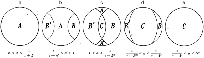
Figure 11: A transcription of von Zeipel’s Figs. Z1–Z5 on his pp. Z369–Z370 (Credit: John Wiley and Sons. Reproduced with permission). a is von Zeipel’s Fig. Z1, b is Z2, c is Z3, d is Z4, and e is Z5. Each of the panels represents the trajectories that the circles (Z45-227) and (Z46-228) make on the $(x,y)=(e\cos g,e\sin g)$ plane. Note that the symbol “I” in the numerators of the figure labels designates perturbing body’s semimajor axis $\left(a^{\prime}\right)$ which is defined as 1 in von Zeipel (1910). On the other hand, the same symbol “I” in the denominators is a non-dimensional number, just equivalent to 1. For example, $\frac{{\rm I}}{{\rm I}+k^{\prime}}$ in a actually means $\frac{a^{\prime}}{1+k^{\prime}}$. Note also that in this figure von Zeipel assumes $k^{\prime}=\frac{1}{2}$ for an expository purpose.

Section Z14 is devoted to describing the characteristics of $R$ when the orbits of the perturbed and perturbing bodies intersect. Since von Zeipel mentions this subject later again in Section Z24 in Chapter IV, let us just make a brief summary. The orbit intersection between the perturbing body on a circular orbit and the perturbed body can happen at the heliocentric distance of $a^{\prime}$ (the semimajor axis of the perturbing body). Let us cite von Zeipel’s original words on this subject:

“It is important to study the character of the function $R$ if the orbits intersect. Obviously, for the orbits that intersect, it is necessary and sufficient that one or other of the following conditions is met:

$${\mbox{1) }}1 =\frac{a\left(1-e^{2}\right)}{1\pm e\cos g}$$

$${\mbox{2) }}e =k^{\prime}$$

and that, moreover, $a$ satisfies the inequality

$$\frac{1}{1+k^{\prime}}<a<\frac{1}{1-k^{\prime}}.$$

The first of these conditions expresses that $r=1$ when $w=-g$ or when $w=\pi-g$.” (p. Z369)

Recall that $w$ seen in von Zeipel’s above statement is true anomaly. Note also that by the definition of the unit of mass, his above equation uses “1” on the left-hand side of the condition “1)” instead of $a^{\prime}$. This distance condition is seen in modern literature (e.g. Babadzhanov and Obrubov, 1992; Farinella et al., 2001; Jopek and Bronikowska, 2017) in a more general form such as

$$a^{\prime}=\frac{a\left(1-e^{2}\right)}{1\pm e\cos g}.$$ (226)

In the denominator of the right-hand term of Eq. (226), the positive sign applies when the orbit intersection occurs at the ascending node of the perturbed body (when $w=-g$). The negative sign applies when the orbit intersection occurs at the descending node of the perturbed body (when $w=\pi-g$).

As for the condition “2) $e=k^{\prime}$” in von Zeipel’s description, we do not follow him well. He wrote “for the orbits that intersect, it is necessary and sufficient that one or other of the following conditions is met.” However, the condition $e=k^{\prime}$ just describes the maximum eccentricity of the perturbed body, not making any constraints on the orbit (in other words, semimajor axis) of the perturbing body. Therefore we have no idea why von Zeipel described $e=k^{\prime}$ as one of the necessary and sufficient conditions for an orbit intersection to happen between the perturbed and perturbing bodies.

The inequality that von Zeipel leaves in the above statement can also be more generally rewritten using the semimajor axis $a^{\prime}$ of the perturbing body as

$$\frac{a^{\prime}}{1+k^{\prime}}<a<\frac{a^{\prime}}{1-k^{\prime}}.$$ (227)

We can interpret the condition (227) as follows. For an orbit intersect to occur, the smallest value of the perihelion distance of the perturbed body $a\left(1-k^{\prime}\right)$ must be smaller than the semimajor axis of the perturber $a^{\prime}$ (i.e. $a<\frac{a^{\prime}}{1-k^{\prime}}$), and the largest value of the aphelion distance $a\left(1+k^{\prime}\right)$ of the perturbed body must be larger than $a^{\prime}$ (i.e. $\frac{a^{\prime}}{1+k^{\prime}}<a$).

Here von Zeipel introduces a pair of new variables $x=e\cos g$ and $y=e\sin g$ for rewriting the above condition “1)” (equivalent to Eq. (227)). Let us literally cite his words:

“By introducing the variables

$$x=e\cos g,\quad y=e\sin g$$

the relation 1) can be written

$$\left(x\pm\frac{1}{2a}\right)^{2}+y^{2}=\left(1-\frac{1}{2a}\right)^{2}.$$ (Z45-227)

This is the equation of two circles whose centers are at the points $x=\mp\frac{1}{2a}$, $y=0$ and which pass, one by the point $x=-1$, $y=0$, the other by the point $x=1$, $y=0$.

The position of the circle (Z45) relative to the circle

$$x^{2}+y^{2}={k^{\prime}}^{2}$$ (Z46-228)

that limits the domain (Z43), depends on the values of $a$ and $k$.” (pp. Z369–Z370)

As before, Eq. (Z45-227) can be rewritten in a more general form using $a^{\prime}$ as

$$\left(x\pm\frac{a^{\prime}}{2a}\right)^{2}+y^{2}=\left(1-\frac{a^{\prime}}{2a}\right)^{2}.$$ (230)

As von Zeipel writes, Eq. (230) produces a pair of circles on the $(x,y)$ plane whose center and radii depend just on $\frac{a}{a^{\prime}}$. The geometric circumstance of the orbit intersection is expressed on the $(x,y)$ plane through the locations of the circles (Z45-227) and another circle (Z46-228). The circle (Z46-228) represents the outermost boundary of the possible motion range of the perturbed body on the $(x,y)$ plane.

von Zeipel graphically illustrates the circumstance that the circles (Z45-227) and (Z46-228) depict in his Figs. Z1–Z5 (pp. Z369–Z370), using $k^{\prime}=\frac{1}{2}$ as an example (note that the value of $k^{\prime}$ just affects the circle (Z46-228), not the circles (Z45-227)). We transcribed these figures as Fig. 11. Let us explain, in a more general way, the geometric condition that each panel of Fig. 11 implies. Recalling the fact that $k^{\prime}$ denotes the maximum of the perturbed body’s eccentricity in the considered system, we use the following notation:

$$Q_{\rm max} =a\left(1+k^{\prime}\right),$$ (231)

$$q_{\rm min} =a\left(1-k^{\prime}\right),$$ (232)

$$\ell_{\rm min} =a\left(1-{k^{\prime}}^{2}\right),$$ (233)

where $Q_{\rm max}$ is the largest value of the perturbed body’s apocenter distance, $q_{\rm min}$ is the smallest value of the perturbed body’s pericenter distance, and $\ell_{\rm max}$ is the smallest value of the perturbed body’s semilatus rectum.

• Fig. 11a: $0<a<\frac{a^{\prime}}{1+k^{\prime}}$. We can interpret this as $0<a$ and $Q_{\rm max}<a^{\prime}$. $0<a$ is obvious, and $Q_{\rm max}<a^{\prime}$ is satisfied if the perturbed body’s orbit always lies inside that of the perturbing body. Hence in this case, the two orbits never intersect. This orbit configuration is similar to that between the Atira asteroids (also known as interior-Earth objects) and the Earth’s orbit (e.g. Greenstreet et al., 2012; Ribeiro et al., 2016; de la Fuente Marcos and de la Fuente Marcos, 2018).

• Fig. 11b: $\frac{a^{\prime}}{1+k^{\prime}}<a<a^{\prime}$. We can interpret this as $a^{\prime}<Q_{\rm max}$ and $a<a^{\prime}$. In this case, the two orbits can intersect. This orbit configuration is similar to that between the Aten near-Earth asteroids and the Earth’s orbit (e.g. Shoemaker et al., 1979; Bottke et al., 2002a).

• Fig. 11c: $a^{\prime}<a<\frac{a^{\prime}}{1-{k^{\prime}}^{2}}$. We can interpret this as $a^{\prime}<a$ and $\ell_{\rm min}<a^{\prime}$. In this case, the two orbits can intersect each other.

• Fig. 11d: $\frac{a^{\prime}}{1-{k^{\prime}}^{2}}<a<\frac{a^{\prime}}{1-k^{\prime}}$. We can interpreted this as $a^{\prime}<\ell_{\rm min}$ and $a^{\prime}>q_{\rm min}$. If we combine the two conditions c and d, and write them as $a^{\prime}<a$ and $a^{\prime}>q_{\rm min}$, this orbit configuration is now close to that between the Apollo near-Earth asteroids and the Earth’s orbit (e.g. Shoemaker et al., 1979; Bottke et al., 2002a).

• Fig. 11e: $\frac{a^{\prime}}{1-k^{\prime}}<a<\infty$ . We can interpret this as $a^{\prime}<q_{\rm min}$ and $a<\infty$. $a<\infty$ is obvious, and the perturbed body’s orbit always lies outside that of the perturbing body if $a^{\prime}<q_{\rm min}$. Hence in this case, the two orbits never intersect each other. This orbit configuration is close to that between the Amor near-Earth asteroids and the Earth’s orbit (e.g. Shoemaker et al., 1979; Bottke et al., 2002a).

To facilitate the reader’s understanding, based on Eqs. (Z45-227) and (Z46-228) we present, as Fig. 12, diagrams of this kind with several more values of $\alpha$. We adopted $k^{\prime}=\frac{1}{2}$ following von Zeipel’s figures. Now we can better see the relation between the $\alpha$ values and the topological configurations of circles. Among the nine values of $\alpha=\frac{a}{a^{\prime}}$ in Fig. 12, the following four depict configurations when the relative topology of the three circles changes: $\alpha=\frac{2}{3}=\frac{1}{1+k^{\prime}}$, $\alpha=1$, $\alpha=\frac{4}{3}=\frac{1}{1-{k^{\prime}}^{2}}$, and $\alpha=2=\frac{1}{1-k^{\prime}}$.

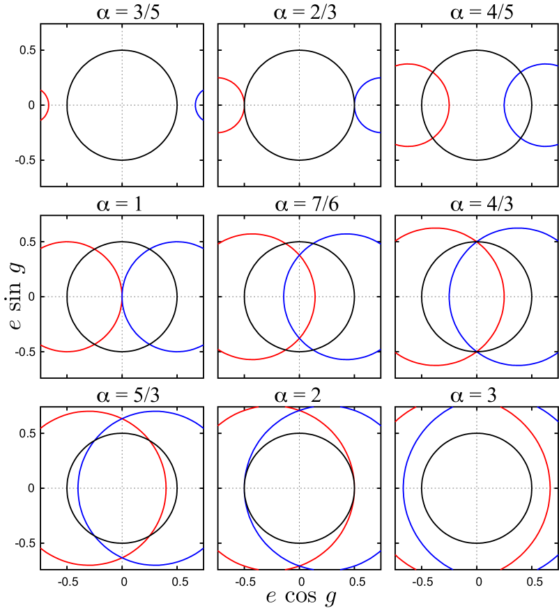
Figure 12: Similar to Fig. 11, we depict circles described by Eqs. (Z45-227) and (Z46-228) with several more values of $\alpha$ on the $(x,y)=(e\cos g,e\sin g)$ plane. The circles drawn in red correspond to the negative sign in the first term of the left-hand side of Eq. (Z45-227). The circles drawn in blue correspond to the positive sign in the first term of the left-hand side of Eq. (Z45-227). The black solid circles at the center are a representation of Eq. (Z46-228). The parameter $k^{\prime}=\frac{1}{2}$ is common to all the panels.

As seen in Fig. 11, von Zeipel named each of the domains as $A$, $A^{\prime}$, $B$, $B^{\prime}$, $C$. In the rest of Section Z14, he tries to prove the following theorem:

“The function $R$ is represented in various domains $A$, $B$, $C$, $A^{\prime}$, $B^{\prime}$ by different analytic functions. Each of these functions is holomorphic in the corresponding domain and on its borders (except the circle $e=k^{\prime}$).” (p. Z369)

The doubly averaged disturbing function $R$ is originally defined as the double integral expressed in Eq. (Z44-224). As a preparation to prove the above theorem, von Zeipel expresses $R$ in a single integral by performing the integration with respect to $\theta^{\prime}$. Although we do not go into his proof of the theorem in this monograph, let us quickly introduce his preparation part because the result is used in a later section (Section Z20; discussed on p. 5.6.3 of this monograph).

von Zeipel first introduces a pair of parameters $\tau$ and $V$ as

$$\left(1+r^{2}\right)\tau\cos V =2r\cos(w+g),$$ (234)

$$\left(1+r^{2}\right)\tau\sin V =2r\sin(w+g)\cos I,$$ (235)

and expresses $\Delta$ in the denominator of Eq. (Z44-224) as follows:

$$\Delta^{2}=\left(1+r^{2}\right)\left[1-\tau\cos\left(\theta^{\prime}+V\right)\right].$$ (Z47-235)

Then the following equation for $\tau^{2}$

$$\tau^{2}=\frac{4r^{2}}{\left(1+r^{2}\right)^{2}}\left[1-\sin^{2}I\sin^{2}(w+g)\right],$$ (Z48-236)

or that for ${\tau^{\prime}}^{2}\equiv 1-\tau^{2}$

$${\tau^{\prime}}^{2}=1-\tau^{2}=\frac{\left(1-r^{2}\right)^{2}+4r^{2}\sin^{2}I\sin^{2}(w+g)}{\left(1+r^{2}\right)^{2}},$$ (Z49-237)

are derived. Now von Zeipel defines a function $F(\tau)$ as

$$\frac{1}{2\pi}\int_{0}^{2\pi}\frac{\sqrt{1+r^{2}}}{\Delta}\theta^{\prime}$$ (Z50-238)

$$\quad=\frac{1}{2\pi}\int_{0}^{2\pi}\frac{d\theta^{\prime}}{\sqrt{1-\tau\cos\left(\theta^{\prime}+V\right)}}=F(\tau).$$

Note that $F(\tau)$ is newly defined in Eq. (Z50-238), but the notation may be confusing. This $F$ is different from the Hamiltonian in Eq. (192). Also, note that $F$ is a function of $\tau$ only, not that of $V$, due to the relation between $V$ and $\tau$ shown in Eqs. (234) and (235).

Now von Zeipel adopts $F(\tau)$ defined in Eq. (Z50-238) for the literal definition of $R$. Changing the integration variable used in the averaging procedure from mean anomaly $l$ to true anomaly $w$ through the commonly used relationship

$$dl=\frac{r^{2}}{a^{2}}\frac{dw}{\sqrt{1-e^{2}}},$$ (240)

he obtains $R$ in the form of a single integral as

$$R=\frac{1}{2\pi}\int_{0}^{2\pi}\frac{r^{2}}{a^{2}}\frac{F(\tau)}{\sqrt{1-e^{2}}\sqrt{1+r^{2}}}dw.$$ (Z51-240)

Note that in Eqs. (240) and (Z51-240) we use $a$, not $\alpha=\frac{a}{a^{\prime}}$. This is for explicitly displaying the quantity $\frac{r}{a}$ as being non-dimensional. However this is just for a formal consistency, because we can practically regard $a$ and $r$ are both non-dimensional from the beginning in von Zeipel’s theory. We already mentioned this point in the discussion following Eq. (188) on p. 5.2 of this monograph.

von Zeipel continues as follows:

“It is well known and easy to verify that $F$ is represented, if $0\leq\tau<1$, by the hypergeometric series,

$$F(\tau)=F\left(\frac{1}{4},\frac{3}{4},1,\tau^{2}\right),$$ (Z52-241)

or by the [complete] elliptic integral of the first kind,

$$F(\tau)=\frac{2}{\pi}\frac{1}{\sqrt{1+\tau}}\int_{0}^{\frac{\pi}{2}}\frac{d\varphi}{\sqrt{1-\frac{2\tau}{1+\tau}\sin^{2}\varphi}}.\mbox{\rm''}$$ (Z53-242)

(p. Z371)

von Zeipel still continues:

“It is also known (see Picard: Traité d’Analysis vol. III, page 273) that $F(\tau)$ is of the form

$$F(\tau)=A\left({\tau^{\prime}}^{2}\right)\log{\tau^{\prime}}^{2}+B\left({\tau^{\prime}}^{2}\right),$$ (Z54-243)

in the neighborhood of $\tau=1$, and both $A$ and $B$ are developed in powers of $\tau^{2}$ with

$$A(0)\neq 0.$$ (Z55-244)

Then $A$, $B$ and $\log{\tau^{\prime}}^{2}$ are real, if $\tau^{2}$ is real and $>0$. Finally we evidently have

$$A(0)<0$$ (Z56-245)

because, if $A(0)>0$, we would have $F(\tau)=-\infty$ for $\tau=1$, which is impossible since $F(\tau)>0$.” (p. Z371)

Nowadays, approximating complete elliptic integrals by a logarithmic function like this is a common idea (e.g. Hastings, Jr., 1955; Cody, 1965a, b). Note that although we found an expression similar to Eq. (Z54-243) in Picard (1896, Chapter XI, sub-chapter II, Section 13, p. 273, as suggested by ), Picard’s original equation is in a more general form. Also, the function that von Zeipel depicted as “$\log$” in Eq. (Z54-243) turned out to be a natural logarithm $(\ln)$ in Picard’s original expression.

Let us wrap up our introduction of von Zeipel’s Section Z14 by citing one of his paragraphs on pp. Z374–Z375. It is about the general characteristics of the secular disturbing function that he deals with:

“According to the formula (Z66), the function $R$ is thus given by two different analytic functions $R^{\prime}$ and $R^{\prime\prime}$ in the two domains $A$ and $B$ in Fig. Z2. Of these functions, $R^{\prime\prime}$ is holomorphic in the domain $A$, and $R^{\prime\prime}$ [is holomorphic] in the domain $B$. Subsequently, the functions $R^{\prime}$ and $R^{\prime\prime}$ are holomorphic also on the arcs of the circles (Z45), which separate the domains $A$ and $B$ from each other, except at the points of intersection of the curves (Z45) and (Z46). Finally, we have $R^{\prime}=R^{\prime\prime}$ on the boundary that separates the domains $A$ and $B$.

In the previous demonstration we have assumed

$$\frac{1}{1+k^{\prime}}<a<1.$$

But it is obviously possible to use the same method almost without change for dealing with

$$1<a<\frac{1}{1+{k^{\prime}}^{2}}$$

and

$$\frac{1}{1-{k^{\prime}}^{2}}<a<\frac{1}{1-k^{\prime}}$$

represented by Figs. Z3 and Z4 on page Z369. To calculate $R$, it is necessary to use different analytic functions in the domains $A$, $B$, $C$, $A^{\prime}$, $B^{\prime}$. These functions are holomorphic in each of the domains $A$, $B$, $C$, $A^{\prime}$, $B^{\prime}$ which they belong to, and also on the borders of this area with an exception of the circle (Z46).” (pp. Z374–Z375)

Note that we have not transcribed von Zeipel’s Eq. (Z66) in this monograph. Note also that in all the three inequalities in the above quotation, “1” in the numerators (not in the denominators) designates the perturbing body’s semimajor axis, $a^{\prime}$. Therefore, the three inequalities can be respectively rewritten as either of the following combinations:

$$\begin{array}[]{cccl}\frac{a^{\prime}}{1+k^{\prime}}<a<a^{\prime},&a^{\prime}<a<\frac{a^{\prime}}{1+{k^{\prime}}^{2}},&\frac{a^{\prime}}{1-{k^{\prime}}^{2}}<a<\frac{a^{\prime}}{1-k^{\prime}},\end{array}$$

or

$$\begin{array}[]{cccl}\frac{1}{1+k^{\prime}}<\alpha<1,&1<\alpha<\frac{1}{1+{k^{\prime}}^{2}},&\frac{1}{1-{k^{\prime}}^{2}}<\alpha<\frac{1}{1-k^{\prime}}.\end{array}$$

See also Fig. 11’s caption and the ensuing discussion.

In the final section (Z15) of Chapter III, von Zeipel mentions the behavior of $R$ close to the outer boundary circle represented by $e=x^{2}+y^{2}=k^{\prime}$ (Z46-228) in a very general way. Although in this monograph we do not go into the contents of this section, we will return to this subject later (Section 5.9.1 on p. 5.9.1) with a more specific function form of $R$ and numerical examples.

Readers should recall that in his Chapter III, von Zeipel’s description is still general. No function form is specified for the secular disturbing function $R$. von Zeipel mentions the specific function form of $R$ for the first time in the following chapter (Chapter IV).

5.6 Secular disturbing function: Inner case

Among von Zeipel’s work in 1910, the chapter “Chapitre IV. Maxima et minima de la partie séculaire de la fonction perturbatrice” comprises the most important component for us. In this chapter he shows an analysis of the doubly averaged disturbing function $R$ with specific function forms. This is what we can directly compare with the later work of Lidov and Kozai in detail.

This chapter is very long, occupying half of the entire article (37 pages out of 74 pages) including ten sections (from Z16 to Z25). We would like to categorize the sections into three parts. For this purpose, we think it is best to cite the beginning part of this chapter in Section Z16:

“In Chapter II we have shown that the integration of the equations (Z12) of the secular variations is much simplified in the vicinity of a maximum or minimum value of the function $R$. It is therefore important to find the points $(e,g)$ of the domain (Z43) for which the function $R$ reaches its maxima and minima.

In the study, that we have in view, it is advantageous to distinguish three cases, characterized by the position of the nodes of the orbit of the infinitesimal mass:

1. Both nodes are located inside the orbit of Jupiter, so that the orbit of the comet remaining in its plane can be reduced to the Sun without intersecting Jupiter’s orbit.

2. Both nodes are located outside the orbit of Jupiter, so that the orbit of the comet remaining in its plane can be reduced to an infinitely large circle around the Sun as the center without touching the orbit Jupiter.

3. Of the two nodes, one is located inside, [and] the other [is located] outside, the orbit of Jupiter. The two orbits behave like the rings of a chain.”

(p. Z378)

In the above, the case 1 is about the inner CR3BP which is discussed in Sections Z16–Z21. The case 2 is about the outer CR3BP which is discussed in Sections Z22–Z23. The case 3 corresponds to a system where orbit intersection between the perturbed and perturbing bodies can happen. This is discussed in Sections Z24–Z25. In the present subsection (Section 5.6), we will summarize von Zeipel’s Sections Z16–Z21 that deal with the case 1.

5.6.1 Expansion of $R$ by $\alpha$

von Zeipel first assumes in Section Z16 that $\alpha=\frac{a}{a^{\prime}}$ is very small. This is equivalent to adopting the quadrupole level approximation, and the expansion of $R$ in the series of $\alpha$ can be truncated at lower-order without losing accuracy. The method that he took for the expansion of $R$ follows Tisserand (1889) that exploits the Hansen coefficients $X_{0}^{2m,2i}$. Omitting the detail, let us transcribe von Zeipel’s expansion result as follows:

$$R =\left[\frac{1}{\Delta}\right]_{l,\theta^{\prime}}=1+\sum_{m=1}^{\infty}\Bigl{(}A_{0.0}^{(2m)}X_{0}^{2m,0}$$ (Z72-246)

$$\qquad\qquad+2\sum_{i=1}^{m}A_{i.j}^{(2m)}X_{0}^{2m,2i}\cos 2ig\Bigr{)}\alpha^{2m},$$

where $\left[\frac{1}{\Delta}\right]_{l,\theta^{\prime}}$ means that the quantity $\frac{1}{\Delta}$ is averaged both by $l$ and by $\theta^{\prime}$. This operation is equivalent to $\left<\left<\frac{1}{\Delta}\right>_{l^{\prime}}\right>_{l}$ that we employed on p. 39 of this monograph.

The Hansen coefficients are expressed as

$$X_{0}^{2m,2i} =\frac{(2m+2i+1)!}{(2m+1)!(2i)!}\left(\frac{e^{2}}{4}\right)^{i}$$ (Z71-247)

$$\times F\left(i-m,i-m-\frac{1}{2},2i+1,e^{2}\right),$$

with

$$A_{i,j}^{(2m)} =k_{i,j}^{(2m)}\left(\frac{\sin^{2}I}{4}\right)^{i}$$ (Z74-248)

$$\times F\left(i-m,i+m+\frac{1}{2},2i+1,\sin^{2}I\right),$$

and

$$k_{i,j}^{(2m)}=\frac{(2m+2i)!(2m)!}{2^{4m}(2i)!(m+i)!(m-i)!(m!)^{2}}.$$ (Z73-249)

Note that $F$ in Eq. (Z71-247) and Eq. (Z74-248) is the hypergeometric series of Gauss.

von Zeipel regards the expansion (Z72-246) as a series of $\alpha^{2}$, and writes down $R$ as

$$R=1+R_{2}\alpha^{2}+R_{4}\alpha^{4}+\cdots,$$ (Z75-250)

where $R_{2}$, $R_{4}$, $\cdots$ are functions of $e$ and $g$. The lowest-order term of $R$ (except for the constant 1) becomes

$$R_{2} =A_{0.0}^{(2)}X_{0}^{2.0}+2A_{1.1}^{(2)}X_{0}^{2.2}\cos 2g$$ (Z76-251)

$$=\frac{1}{4}\left(1-\frac{3}{2}\sin^{2}I\right)\left(1+\frac{3}{2}e^{2}\right)$$

$$\qquad+\frac{15}{16}\sin^{2}I\cdot e^{2}\cos 2g$$

$$=\frac{1}{8}\left(-1+\frac{3k^{2}}{1-e^{2}}\right)\left(1+\frac{3}{2}e^{2}\right)$$

$$\qquad+\frac{15}{16}\left(1-\frac{k^{2}}{1-e^{2}}\right)e^{2}\cos 2g.$$

It is clear that $R_{2}$ in Eq. (Z76-251) is equivalent to what we saw in Kozai’s work (Eq. (72) of this monograph).

Note that von Zeipel actually used $a$ instead of $\alpha=\frac{a}{a^{\prime}}$ throughout his discussion of the inner problem. For example, the original form of Eq. (Z75-250) is written as follows:

$$R=1+R_{2}a^{2}+R_{4}a^{4}+\cdots.$$ (253)

The apparent difference between Eq. (Z75-250) and Eq. (253) comes from the fact that von Zeipel fixes the perturber’s semimajor axis $\left(a^{\prime}\right)$ as 1 (the unit of length in his theory). However, for keeping the generality and compatibility with the later studies by Lidov and Kozai, we use the variable of $\alpha$ instead of just $a$.

Next, using the polar coordinate variables $x=e\cos g$ and $y=e\sin g$, von Zeipel expands $R$ of Eq. (Z75-250) into a two-variable Taylor series of $x^{2}$ and $y^{2}$ as

$$R=R_{0,0}+R_{2.0}x^{2}+R_{0.2}y^{2}+\cdots.$$ (Z77-253)

The coefficients $R_{2.0}$ and $R_{0.2}$ are expanded into the power series of $\alpha^{2}$ as

$$R_{2.0} =\frac{3}{4}\alpha^{2}+P_{4}\alpha^{4}+P_{6}\alpha^{6}+\cdots,$$ (Z78-254)

$$R_{0.2} =\frac{15}{8}\left(k^{2}-\frac{3}{5}\right)\alpha^{2}+Q_{4}\alpha^{4}+Q_{6}\alpha^{6}+\cdots,$$

where $P_{2i}$ and $Q_{2i}$ $(i=2,3,\cdots)$ are polynomials of $k^{2}$, although von Zeipel did not show their actual forms.

von Zeipel did not show the specific form of the first term $R_{0.0}$ in Eq. (Z77-253). But we can calculate it by actually carrying out the two-variable Taylor expansion. We get:

$$R_{0.0}=1+\frac{3k^{2}-1}{8}\alpha^{2}+\cdots.$$ (256)

However, constant terms such as $R_{0.0}$ do not matter in the following discussions. This is because von Zeipel’s major goal was to search for local extremums of $R$ by calculating its partial derivatives such as $\frac{\partial R}{\partial x}$ or $\frac{\partial R}{\partial y}$.

Now von Zeipel defines a new quantity $k^{2}_{0.2}$ as the root of the following equation

$$R_{0.2}=0.$$ (257)

When $\alpha\ll 1$ (i.e. the quadrupole level approximation), we know $k^{2}_{0.2}=\frac{3}{5}$ from Eq. (Z78-254). This number must already be familiar to the readers. von Zeipel further expands $k^{2}_{0.2}$ into the power series of $\alpha^{2}$ as

$$k^{2}_{0.2}=\frac{3}{5}+K_{2}\alpha^{2}+K_{4}\alpha^{4}+\cdots,$$ (Z79-257)

where $K_{2}$, $K_{4}$, $\cdots$ are some numerical coefficients whose actual form von Zeipel did not show. $k^{2}_{0.2}$ later plays a fundamental role in locating the local extremums of $R$.

5.6.2 Search for local extremums

In the rest of Section Z16, von Zeipel tries to find local extremums of $R$ on the $(x,y)=(e\cos g,e\sin g)$ plane by assuming $\alpha\ll 1$. This means that he assumes $k_{0.2}^{2}=\frac{3}{5}$. His general approach here is divided into two stages:

1. He first locates local extremums of $R$ by calculating its first derivatives, such as $\frac{\partial R}{\partial x}$.

2. He then determines whether the discovered local extremum is a local minimum, a local maximum, or a saddle point by inspecting the sign of the second derivatives of $R$ such as $\frac{\partial^{2}R}{\partial x{}^{2}}$.

As we see in what follows, von Zeipel’s search areas for the local extremums are the origin $(x,y)=(0,0)$, the outer boundary $x^{2}+y^{2}={k^{\prime}}^{2}$, and the $y$-axis.

At the origin

von Zeipel first considers the behavior of $R$ at the origin, $(x,y)=(0,0)$. His conclusion is as follows:

• The origin is a local minimum of $R$ when $k^{2}>k^{2}_{0.2}$.

• The origin is a saddle point of $R$ when $k^{2}<k^{2}_{0.2}$.

von Zeipel confirms this as follows. At the origin, from Eqs. (Z77-253) and (Z78-254) we have

$$\frac{\partial R}{\partial x}=\frac{\partial R}{\partial y}=0.$$ (259)

Also, we have

$$\frac{\partial^{2}R}{\partial x{}^{2}} =2R_{2.0}\sim\frac{3}{2}\alpha^{2},$$ (260)

$$\frac{\partial^{2}R}{\partial y{}^{2}} =2R_{0.2}\sim\frac{15}{4}\left(k^{2}-\frac{3}{5}\right)\alpha^{2},$$ (261)

at $(x,y)=(0,0)$ when $\alpha\ll 1$. The relationships (260) and (261) hold true at the origin because the higher-order expansion terms appearing in the Taylor series (Z77-253) all vanish in the second derivatives, just leaving the terms of $2R_{2.0}$ and $2R_{0.2}$ as in Eqs. (260) and (261).

Now from Eqs. (260) and (261), when $k^{2}>k^{2}_{0.2}$ we have

$$\frac{\partial^{2}R}{\partial x{}^{2}}>0,\quad\frac{\partial^{2}R}{\partial y{}^{2}}>0.$$ (262)

This indicates that $R$ has a local minimum at the origin. It is obvious from Eq. (260) that $\frac{\partial^{2}R}{\partial x{}^{2}}>0$ is true regardless of the value of $k^{2}$ in this approximation.

On the other hand when $k^{2}<k^{2}_{0.2}$, from Eqs. (260) and (261) we have at $(x,y)=(0,0)$

$$\frac{\partial^{2}R}{\partial x{}^{2}}>0,\quad\frac{\partial^{2}R}{\partial y{}^{2}}<0.$$ (263)

From Eqs. (262) and (263) we know that $R$ has a saddle point (“minimax” in von Zeipel’s terminology) at the origin.

At the outer boundary

von Zeipel then moves on to a consideration of $R$ on its outer boundary. As we saw before (Section 5.5 on p. Z43-223), $R$ has a constant value on the outer boundary $x^{2}+y^{2}={k^{\prime}}^{2}$, and it is independent of $g$ on this circle. By calculating the partial derivative $\frac{\partial R}{\partial(e^{2})}$ and substituting $e^{2}={k^{\prime}}^{2}=1-k^{2}$ into it, on the boundary circle von Zeipel obtains (p. Z381)

$$\left.\frac{\partial R}{\partial\left(e^{2}\right)}\right|_{e^{2}={k^{\prime}}^{2}}=\left.\alpha^{2}\frac{\partial R_{2}}{\partial\left(e^{2}\right)}\right|_{e^{2}={k^{\prime}}^{2}}+\cdots$$ (264)

$$\quad=\alpha^{2}\frac{3}{16k^{2}}\left[5-k^{2}-5\left(1-k^{2}\right)\cos 2g\right]+\cdots.$$

As long as $\alpha$ is small and the higher-order terms than $\alpha^{2}$ can be ignored, it is clear that the right-hand side of Eq. (264) is always positive (with the smallest value of $4k^{2}$). Hence, at the quadrupole level approximation we have

$$\left.\frac{\partial R}{\partial\left(e^{2}\right)}\right|_{e^{2}={k^{\prime}}^{2}}>0,$$ (265)

on the outer boundary. Equation (265) indicates that, just inside the outer boundary, $R$ continues to increase along the radial direction on the $(x,y)=(e\cos g,e\sin g)$ plane until it reaches $e=k^{\prime}$. In this sense, the outer boundary circle expressed by $x^{2}+y^{2}={k^{\prime}}^{2}$ can be regarded as a kind of local maximum of $R$.

Note that von Zeipel frequently uses $\frac{\partial R}{\partial(e^{2})}$, instead of $\frac{\partial R}{\partial e}$, for determining whether or not a particular point (or a curve) of $R$ makes a local extremum. It may seem strange because the considered phase space is described by the variables $(x,y)=(e\cos g,e\sin g)$. But we suspect his use of $\frac{\partial R}{\partial\left(e^{2}\right)}$ is justified for two reasons. First, the function form of $R$ in Eq. (Z76-251) contains the perturbed body’s eccentricity only in the form of $e^{2}$. Second, whether we use $\frac{\partial R}{\partial\left(e^{2}\right)}$ or $\frac{\partial R}{\partial e}$ would not matter for the purpose of locating local extremums of $R$. This is due to the identity

$$\frac{\partial R}{\partial e}=2e\frac{\partial R}{\partial\left(e^{2}\right)}.$$ (266)

Therefore, we see that $\frac{\partial R}{\partial\left(e^{2}\right)}\lesseqgtr 0$ always leads to $\frac{\partial R}{\partial e}\lesseqgtr 0$ as long as $e>0$. Thus we find that searching for the locations where $\frac{\partial R}{\partial e}=0$ is realized is equivalent to searching for the locations where $\frac{\partial R}{\partial\left(e^{2}\right)}=0$ is realized.

Along the $y$-axis

Now von Zeipel moves on to the search for local maxima or minima which may be located somewhere between the origin $(x,y)=(0,0)$ and the outer boundary circle $\bigl{(}x^{2}+y^{2}={k^{\prime}}^{2}\bigr{)}$. For this purpose, the following equations must be solved in general:

$$\frac{\partial R}{\partial\left(e^{2}\right)}=0,\quad\frac{\partial R}{\partial g}=0.$$ (Z80-266)

We should bear in mind that $R\sim R_{2}$ as long as $\alpha\ll 1$.

It is clear that the differential operation $\frac{\partial R_{2}}{\partial g}$ eliminates the first term of $R_{2}$ in Eq. (Z76-251), and just leaves its second term. The second term of $R_{2}$ in Eq. (Z76-251) yields a factor of $\sin 2g$ through the operation $\frac{\partial R_{2}}{\partial g}$, so the roots of the equation $\frac{\partial R}{\partial g}=0$ in Eq. (Z80-266) occur when $\sin 2g=0$. This means $\cos 2g=+1$ or $\cos 2g=-1$.

When $\cos 2g=+1$, $\frac{\partial R}{\partial\left(e^{2}\right)}$ becomes (in the second equation from the top on p. Z382)

$$\frac{\partial R}{\partial\left(e^{2}\right)} =\alpha^{2}\frac{\partial R_{2}}{\partial\left(e^{2}\right)}+\cdots$$ (268)

$$=\frac{3}{4}\alpha^{2}+O\left(\alpha^{4}\right).$$

The quantity in the right-hand side of Eq. (268) is always greater than zero when $\alpha\ll 1$. This indicates that the first equation of Eq. (Z80-266) does not have any solution. It means that, along the axis that satisfies $\cos 2g=+1$, $R$ (or $R_{2}$) monotonically increases from the origin toward the outer boundary without any local extremums.

On the other hand when $\cos 2g=-1$, $\frac{\partial R}{\partial\left(e^{2}\right)}$ becomes (in the third equation on p. Z382)

$$\frac{\partial R}{\partial\left(e^{2}\right)} =\alpha^{2}\frac{\partial R_{2}}{\partial\left(e^{2}\right)}+\cdots$$ (269)

$$=\alpha^{2}\left(-\frac{9}{8}+\frac{15}{8}k^{2}\frac{1}{\left(1-e^{2}\right)^{2}}\right)+O\left(\alpha^{4}\right).$$

The quantity in the right-hand side of Eq. (269) can be either positive or negative depending on the value of $k^{2}$. It leaves a possibility for local extremums to occur. Then, von Zeipel expresses the solution of the equation $\frac{\partial R}{\partial\left(e^{2}\right)}=0$ as:

$$e^{2}=e^{2}_{0.2}=1-\sqrt{\frac{5}{3}k^{2}}+c_{2}\alpha^{2}+c_{4}\alpha^{4}+\cdots,$$ (Z81-269)

where $c_{2}$, $c_{4}$, $\cdots$ are polynomials of $k$ whose function form he did not show. Equation (Z81-269) means that $R$ can have a pair of local extremums at the points $(x,y)=(0,\pm e_{0.2})$, or in other words, at $(e,g)=(e_{0.2},\pm\frac{\pi}{2})$. In p. Z382 von Zeipel also introduces the equation

$$e^{2}_{0.2}=0,$$ (271)

together with a formal solution that satisfies Eq. (271) as

$$k^{2}=\overline{k_{0.2}}^{2}=\frac{3}{5}+K^{\prime}_{2}\alpha^{2}+K^{\prime}_{4}\alpha^{4}+\cdots,$$ (272)

where $K^{\prime}_{2}$, $K^{\prime}_{4}$ are some numerical coefficients.

Note that in von Zeipel’s original notation (p. Z382), $\overline{k_{0.2}}^{2}$ in Eq. (272) is denoted as ${k^{\prime}}^{2}_{0.2}$. However, ${k^{\prime}}^{2}_{0.2}$ is used later for a different purpose (Eq. (Z100-327) on p. 5.7.2 of this monograph). For avoiding the probable confusion that readers might have, in this monograph we have altered the notation from ${k^{\prime}}^{2}_{0.2}$ to $\overline{k_{0.2}}^{2}$ in Eq. (272). Note also that von Zeipel did not mention at all what $K^{\prime}_{2}$, $K^{\prime}_{4}$, $\cdots$ in Eq. (272) are. Their function forms are not shown either. We interpret they are some numerical coefficients similar to those $(K_{2},K_{4},\cdots)$ in Eq. (Z79-257).

From Eq. (Z81-269) it is straightforward to understand that $k^{2}<\frac{3}{5}$ is necessary for $e^{2}_{0.2}$ to be positive, as long as $\alpha\ll 1$. When $k^{2}=\frac{3}{5}$, we have $e^{2}_{0.2}=0$, and the positions of the local extremums converge into the origin $(0,0)$. When $k^{2}>\frac{3}{5}$, we have $e^{2}_{0.2}<0$, and $e_{0.2}$ cannot be a real number. Therefore, we find $k^{2}<\frac{3}{5}$ as a condition for local extremums to show up on the $y$-axis (but except at the origin). It is also obvious that the value $\frac{3}{5}$ is equivalent to $k^{2}_{0.2}$ described in Eq. (Z79-257) as long as $\alpha\ll 1$.

Now von Zeipel starts his examination of the type of the local extremums at $(x,y)=(0,\pm e_{0.2})$; in other words, at $(e,g)=(e_{0.2},\pm\frac{\pi}{2})$. Which type of local extremum would $R$ take at these points, local minima or maxima?

Type of the local extremum on the $y$-axis

For examining the characteristics of the points $(e,g)=(e_{0.2},\pm\frac{\pi}{2})$ as local extremums of $R$, von Zeipel focuses on the sign of the second derivatives of $R$ at $\cos 2g=-1$. They are $\frac{\partial^{2}R}{\partial g{}^{2}}$, $\frac{\partial^{2}R}{\partial e\partial g}$, and $\frac{\partial^{2}R}{\partial e{}^{2}}$.

As for $\frac{\partial^{2}R}{\partial g{}^{2}}$, from Eq. (Z76-251) we have

$$\left.\frac{\partial^{2}R}{\partial g{}^{2}}\right|_{\cos 2g=-1}=\frac{15}{4}e^{2}\sin^{2}I,$$ (274)

which is clearly larger than, or equal to, zero.

As for $\frac{\partial^{2}R}{\partial e\partial g}$, it is also clear that

$$\left.\frac{\partial^{2}R}{\partial e\partial g}\right|_{\cos 2g=-1}=0.$$ (275)

$\frac{\partial^{2}R}{\partial e{}^{2}}$ is slightly complicated, and von Zeipel’s original description seems too terse. Let us try to add a complementary description as to how we should deal with $\frac{\partial^{2}R}{\partial e{}^{2}}$.

von Zeipel shows an identity on p. Z383 as

$$\frac{\partial^{2}R}{\partial^{2}e}\equiv 2\frac{\partial R}{\partial\left(e^{2}\right)}+4e^{2}\frac{\partial^{2}R}{\partial\left(e^{2}\right)^{2}}.$$ (276)

Adopting Eq. (276) for $\frac{\partial^{2}R}{\partial e{}^{2}}$, we get

$$\left.\frac{\partial^{2}R}{\partial e{}^{2}}\right|_{\cos 2g=-1} =\frac{3}{4\left(1-e^{2}\right)^{3}}$$ (277)

$$\times \left(3e^{6}-9e^{4}+9e^{2}+5k^{2}\left(3e^{2}+1\right)-3\right).$$

By substituting the eccentricity value ($e=e_{0.2}$ of Eq. (Z81-269)) at the considered points into Eq. (277), we get

$$\left.\frac{\partial^{2}R}{\partial e{}^{2}}\right|_{\cos 2g=-1,e=e_{0.2}}=\frac{9}{5}\sqrt{\frac{15}{k^{2}}}-9.$$ (278)

Equation (278) means that, at $\cos 2g=-1$, $\frac{\partial^{2}R}{\partial e{}^{2}}$ monotonically decreases as $k^{2}$ increases. But it remains positive while $k^{2}<\frac{3}{5}$. Here we must remember that, as mentioned before, $k^{2}<\frac{3}{5}$ is the necessary condition for $e^{2}_{0.2}$ to exist as a positive number (see Eq. (Z81-269)). Therefore in this range of $k^{2}$, we have the following:

$$\left.\frac{\partial^{2}R}{\partial e{}^{2}}\right|_{\cos 2g=-1,e=e_{0.2}}>0.$$ (279)

In summary, the three second derivatives (274), (275), and (279) indicate that $R$ takes local minima on the $(x,y)$ plane when $\cos 2g=-1$. Their coordinates are $(x,y)=(0,\pm e_{0.2})$; in other words, $(e,g)=(e_{0.2},\pm\frac{\pi}{2})$.

Taking into account all the results that have been obtained, von Zeipel states the following proposition:

“That being so, we can state the following proposition as demonstrated:

If $\alpha$ is small and $k^{2}_{0.2}<k^{2}<1$, the function $R$ possesses one minimum value in the domain (Z43), located at the point $e=0$. — Instead, if $\alpha$ being small, we have $0<k^{2}<k^{2}_{0,2}$, then $R$ has a minimax at the origin and its only minimum value in the domain (Z43) at the two symmetric points $g=\pm\frac{\pi}{2}$, $e=e_{0.2}$. — Finally, the constant value that $R$ takes on the circle $e=k^{\prime}$ is the largest value in the domain (Z43); and there is no other maximum value for $R$ in this domain.” (p. Z383)

After these considerations, von Zeipel presents two schematic plots of equi-$R$ curves on the $(e\cos g,e\sin g)$ plane as his Figs. Z6 and Z7 for illustrating the circumstances. We transcribed them as our Fig. 13. Through his figures, it is obvious that the topology of the equi-$R$ contours qualitatively changes across $k^{2}=k^{2}_{0.2}$. Recalling the fact that $k^{2}_{0.2}=\frac{3}{5}$ when $\alpha\ll 1$, it is evident that von Zeipel’s schematic plots in Fig. 13 are exactly about what Lidov and Kozai reached at the quadrupole level approximation. See Fig. 8 of this monograph for comparison.

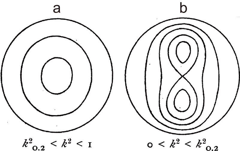
Figure 13: Transcription of von Zeipel’s Figs. Z6 and Z7 on his p. Z384 (Credit: John Wiley and Sons. Reproduced with permission). They represent schematic trajectories of equi-$R$ contours of the doubly averaged inner CR3BP on the $(e\cos g,e\sin g)$ plane. a: von Zeipel’s Fig. Z6, showing the status when $k^{2}_{0.2}<k^{2}<1$. b: von Zeipel’s Fig. Z7, showing the status when $0<k^{2}<k^{2}_{0.2}$.

5.6.3 When $\alpha$ is not so small

In the subsequent sections from Z17 to Z21, von Zeipel deals with the doubly averaged inner CR3BP when the semimajor axis ratio $\alpha=\frac{a}{a^{\prime}}$ is not negligibly small. He takes care of this problem through a kind of numerical method. His discussions in what follows begin with an examination of the behavior of $R$ at the origin $(x,y)=(0,0)$. Then he moves on to a consideration of the dynamical characteristics of several asteroids that actually exist in the solar system. After that, he returns to considering the behavior of $R$ along the $y$-axis.

At the origin

von Zeipel first goes on to consider whether or not $R$ takes a local minimum at the origin $(0,0)$, even when $\alpha$ is not so small. This is the objective of his Section Z17. For this purpose von Zeipel expands $R_{2.0}$ and $R_{0.2}$ using the Laplace coefficients, in a different way from what he demonstrated in Eqs. (Z72-246), (Z77-253), and (Z78-254). This is because von Zeipel thought the series expansion Eq. (Z72-246) converges too slowly when $\alpha$ is not small. Nowadays, this is rather a famous fact in the context of comparison between expansions of the disturbing function using the Legendre polynomials and that using the Laplace coefficient (e.g. Farago and Laskar, 2010). The advantage of the former expansion is that there is no restriction in the value range of eccentricity in the secular form of the disturbing function, whereas the latter requires truncation at some order of eccentricity. As a result, von Zeipel’s expansions of $R_{2.0}$ and $R_{0.2}$ in this section seem limited to $O\left(e^{2}\right)$. We do not get into the detail of the elaborate formulations that von Zeipel develops in Section Z17, and we confine ourselves to introducing only the major formulas that he showed. von Zeipel’s formulations in this section rely largely on the legacy of celestial mechanics developed in the nineteenth century, in particular, by Tisserand and Jacobi.

von Zeipel first introduces a set of new coefficients $c^{i,k}$ and $e^{i,k}$, and shows how $R_{2.0}$ and $R_{0.2}$ are expressed by these. $c^{i,k}$ and $e^{i,k}$ are defined as follows (pp. Z383–Z384):

$$\left[1+\alpha^{2}-2\alpha\left(\mu\cos M+\nu\cos N\right)\right]^{-\frac{3}{2}}$$

$$\quad=c^{0.0}+2c^{1.0}\cos M+2c^{0.1}\cos N$$

$$\quad\quad+4c^{1.1}\cos M\cos N+\cdots,$$ (280)

$$\left[1+\alpha^{2}-2\alpha\left(\mu\cos M+\nu\cos N\right)\right]^{-\frac{5}{2}}$$

$$\quad=e^{0.0}+2e^{1.0}\cos M+2e^{0.1}\cos N$$

$$\quad\quad+4e^{1.1}\cos M\cos N+\cdots.$$ (281)

where

$$M=u+\theta^{\prime},\quad N=u-\theta^{\prime},$$ (282)

$$\mu+\nu=1,\quad\mu-\nu=k,$$ (283)

and $u$ is eccentric anomaly. Note that $e^{i,k}$ in Eq. (281) is not directly related to eccentricity $e$. Note also that $\mu$ in Eq. (283) is not Jupiter’s mass. $\nu$ in Eq. (283) is also a newly defined parameter, and it does not have anything to do with what showed up in earlier chapters.

Using eccentric anomaly $u$, von Zeipel obtains an expression of the doubly averaged disturbing function $R$ as

$$R =\frac{1}{4\pi^{2}}\int_{0}^{2\pi}\int_{0}^{2\pi}\frac{1}{\Delta}dld\theta^{\prime}$$

$$=\frac{1}{4\pi^{2}}\int_{0}^{2\pi}\int_{0}^{2\pi}\frac{1-e\cos u}{\Delta}dud\theta^{\prime},$$ (Z83-283)

with

$$\Delta^{2} =1+r^{2}$$

$$-2r\left[\cos(w+g)\cos\theta^{\prime}-\sin(w+g)\sin\theta^{\prime}\cos I\right].$$ (285)

Note that $w$ is the true anomaly of the perturbed body.

Now von Zeipel puts $g=0$ in order to obtain the expression of $R_{2.0}$ that showed up in Eq. (Z77-253). We presume that the substitution of $g=0$ into Eq. (Z83-283) is justified, because $R_{2.0}$ serves as the amplitude of the $x^{2}$-component of $R$ along the $x$-axis by its definition (Z77-253). Therefore only $R_{2.0}$ matters along the $x$-axis $\left(g=0,\pi\right)$, and only $R_{0.2}$ matters along the $y$-axis $\left(g=\pm\frac{\pi}{2}\right)$ as long as $e^{2}$ (hence $x^{2}$ and $y^{2}$) is small. By putting $g=0$, von Zeipel obtains an expression for $\Delta$ in Eq. (285) as

$$\Delta^{2} =1+\alpha^{2}(1-e\cos u)^{2}$$ (286)

$$-2\alpha\left[\mu\cos\left(u+\theta^{\prime}\right)+\nu\cos\left(u-\theta^{\prime}\right)-e\cos\theta^{\prime}\right].$$

Then he defines a new variable

$$\Delta^{2}_{0}=1+\alpha^{2}-2\alpha\left[\mu\cos\left(u+\theta^{\prime}\right)+\nu\cos\left(u-\theta^{\prime}\right)\right],$$ (287)

and obtains the following expansion

$$\frac{1-e\cos u}{\Delta}=\frac{1}{\Delta_{0}}+e\left(-\frac{\cos u}{\Delta_{0}}+\frac{\alpha^{2}\cos u}{\Delta_{0}^{3}}-\frac{\alpha\cos\theta^{\prime}}{\Delta_{0}^{3}}\right)$$ (288)

$$+e^{2}\left(-\frac{3}{2}\frac{\alpha^{2}\cos^{2}u}{\Delta_{0}^{3}}+\frac{\alpha\cos u\cos\theta^{\prime}}{\Delta_{0}^{3}}+\frac{3}{2}\frac{\alpha^{4}\cos^{2}u}{\Delta_{0}^{5}}\right.$$

$$\left.-3\frac{\alpha^{3}\cos u\cos\theta^{\prime}}{\Delta_{0}^{5}}+\frac{3}{2}\frac{\alpha^{2}\cos^{2}\theta^{\prime}}{\Delta_{0}^{5}}\right)+\cdots.$$

Now, we find that $\Delta_{0}^{-3}$ and $\Delta_{0}^{-5}$ appearing in Eq. (288) can be expressed by the coefficients $c^{i,k}$ and $e^{i,k}$ defined in Eqs. (280) and (281). von Zeipel eventually finds the expanded form of $R_{2.0}$ as follows:

$$R_{2.0}= -\frac{3}{4}\alpha^{2}\left(c^{0.0}+c^{1.1}\right)+\frac{1}{2}\alpha\left(c^{1.0}+c^{0.1}\right)$$ (Z85-288)

$$+\frac{3}{4}\alpha^{2}\left(1+\alpha^{2}\right)\left(e^{0.0}+e^{1.1}\right)$$

$$-\frac{3}{2}\alpha^{3}\left(e^{1.0}+e^{0.1}\right).$$

A similar procedure is applied to $R_{0.2}$. Since $R_{0.2}$ serves as the amplitude of the $y^{2}$-component of $R$ along the $y$-axis by its definition (Z72-246), we should assume $g=\frac{\pi}{2}$ or $g=-\frac{\pi}{2}$ for obtaining the expression of $R_{0.2}$. By placing $g=\frac{\pi}{2}$ and going through the same procedure, von Zeipel reaches the following expression for $R_{0.2}$ as

$$R_{0.2}= -\frac{3}{4}\alpha^{2}\left(c^{0.0}-c^{1.1}\right)+\frac{3}{4}\alpha k\left(c^{1.0}-c^{0.1}\right)$$ (Z87-289)

$$-\frac{1}{4}\alpha\left(c^{1.0}+c^{0.1}\right)+\frac{3}{4}\alpha^{4}\left(e^{0.0}-e^{1.1}\right)$$

$$-\frac{3}{2}\alpha^{3}k\left(c^{1.0}-c^{0.1}\right)+\frac{3}{4}\alpha^{2}k^{2}\left(c^{0.0}-c^{1.1}\right).$$

Now, he brings up the following recursion formulas between $c^{i.k}$ and $e^{i.k}$ by citing Jacobi’s Gesammelte Werke, vol. 6, p. 140 (Weierstrass, 1891):

$$3c^{0.0}+c^{1.1}$$

$$\quad=3\left(1+\alpha^{2}\right)\left(e^{0.0}-e^{1.1}\right)-6\alpha\left(\mu-\nu\right)\left(e^{1.0}-e^{0.1}\right),$$ (291)

$$3c^{0.0}-c^{1.1}$$

$$\quad=3\left(1+\alpha^{2}\right)\left(e^{0.0}+e^{1.1}\right)-6\alpha\left(\mu+\nu\right)\left(e^{1.0}+e^{0.1}\right).$$ (292)

Using Eqs. (291) and (292), von Zeipel simplifies Eqs. (Z85-288) and (Z87-289) as follows:

$$R_{2.0} =-\alpha^{2}c^{1.1}+\frac{1}{2}\alpha\left(c^{1.0}+c^{0.1}\right),$$ (Z88-292)

$$R_{0.2} =\alpha^{2}c^{1.1}-\frac{1}{4}\alpha\left(c^{1.0}+c^{0.1}\right)$$

$$+\frac{3}{4}\alpha k\left(c^{1.0}-c^{0.1}\right)-\frac{3}{4}\alpha^{2}\left(1-k^{2}\right)\left(e^{0.0}-e^{1.1}\right).$$

Then von Zeipel expands $c^{i.k}$ and $e^{i.k}$ into a power series of $\alpha$ assuming $|\alpha|<1$ (here he cites Poincaré (1907, p. 111)), but not in the manner of Eq. (Z72-246) because of its slow convergence when $\alpha$ is not small. Instead, he introduces new coefficients $b^{i.k}$ defined as

$$\left[1+\alpha^{2}-2\alpha\left(\mu\cos M+\nu\cos N\right)\right]^{-\frac{1}{2}}$$ (294)

$$=b^{0.0}+2b^{1.0}\cos M+2b^{0.1}\cos N$$

$$+4b^{1.1}\cos M\cos N+\cdots,$$

and calculates $c^{i.k}$ and $e^{i.k}$ using the recursion formulas provided by Jacobi (Gesammelte Werke, vol. 6, p. 142) as

$$\varepsilon =\alpha+\frac{1}{\alpha},$$ (Z89-294)

$$c^{0.0}+c^{1.1} =\frac{\varepsilon\left(b^{0.0}-3b^{1.1}\right)-2\left(b^{1.0}+b^{0.1}\right)}{\alpha\left(\varepsilon^{2}-4\right)},$$

$$c^{0.0}-c^{1.1} =\frac{\varepsilon\left(b^{0.0}+3b^{1.1}\right)-2k\left(b^{1.0}-b^{0.1}\right)}{\alpha\left(\varepsilon^{2}-4k^{2}\right)},$$

$$c^{1.0}+c^{0.1} =\frac{2\left(b^{0.0}-3b^{1.1}\right)-\varepsilon\left(b^{1.0}+b^{0.1}\right)}{\alpha\left(\varepsilon^{2}-4\right)},$$

$$c^{1.0}-c^{0.1} =\frac{2k\left(b^{0.0}+3b^{1.1}\right)-\varepsilon\left(b^{1.0}-b^{0.1}\right)}{\alpha\left(\varepsilon^{2}-4k^{2}\right)},$$

$$e^{0.0}-e^{1.1} =\frac{\varepsilon\left(3c^{0.0}+c^{1.1}\right)+2k\left(c^{1.0}-c^{0.1}\right)}{3\alpha\left(\varepsilon^{2}-4k^{2}\right)}.$$

Here von Zeipel obtains the expressions of $b^{0.0}$, $b^{1.0}$, $b^{0.1}$, $b^{1.1}$ with the aid of Tisserand (1889, note that cites pp. 444–447 (Sections 191 and 192 in Chapter XXVIII) of this book, but no equivalent expression to Eq. (Z90-295) is found there) as follows:

$$b^{0.0} =\frac{1}{2}b^{(0)}+\sum_{m=1}^{\infty}b^{(2m)}Q_{0.0}^{(2m)},$$ (Z90-295)

$$b^{0.1} =\sum_{m=1}^{\infty}b^{(2m-1)}Q_{0.1}^{(2m-1)},$$

$$b^{1.0} =\sum_{m=1}^{\infty}b^{(2m-1)}Q_{1.0}^{(2m-1)},$$

$$b^{1.1} =\sum_{m=1}^{\infty}b^{(2m)}Q_{1.1}^{(2m)},$$

where $b^{(i)}$ are (according to von Zeipel) the Laplace coefficients. The definition of $Q_{i.j}$ are shown later.

Note that what von Zeipel calls the Laplace coefficients $b^{(i)}$ in Eq. (Z90-295) seems slightly different from what we now see in modern textbooks (e.g. Brouwer and Clemence, 1961, p. 495) because there is no subscript such as $b^{(i)}_{s}$. From the definition of $b^{i.k}$ in Eq. (294), we suspect that von Zeipel’s $b^{(i)}$ is equivalent to $b^{(i)}_{\frac{1}{2}}$ in modern textbooks: The Laplace coefficients with the smallest subscript.

Next von Zeipel calculates the function $Q_{i.j}^{(n)}$ in Eq. (Z90-295) which depends only on $\mu$ and $\nu$. For this purpose he employed the following relationships (Z(c)-296), (Z(c)-296), (Z(c)-296) originally seen in Tisserand (1889, Chapter XXVIII, p. 447, p. 452, and p. 456):

$$2Q_{i.j}^{(n)}=R_{i.j}^{(n)}-R_{i.j}^{(n-2)},$$ (Z(c)-296)

$$R_{i,j}^{(n)} =c_{i.j}^{(n)}\mu^{i}\nu^{j}$$ (Z(d)-297)

$$\times F^{2}\left(\frac{i+j-n}{2},\frac{i+j+n+2}{2},j+1,\nu\right),$$

$$c_{i,j}^{(n)}=\frac{\Pi\left(\frac{n+i+j}{2}\right)\Pi\left(\frac{n-i+j}{2}\right)}{\left[\Pi(j)\right]^{2}\Pi\left(\frac{n+i-j}{2}\right)\Pi\left(\frac{n-i-j}{2}\right)},$$ (Z(e)-298)

where

$$\Pi(s)=1\cdot 2\cdot 3\cdots s=s!.$$ (300)

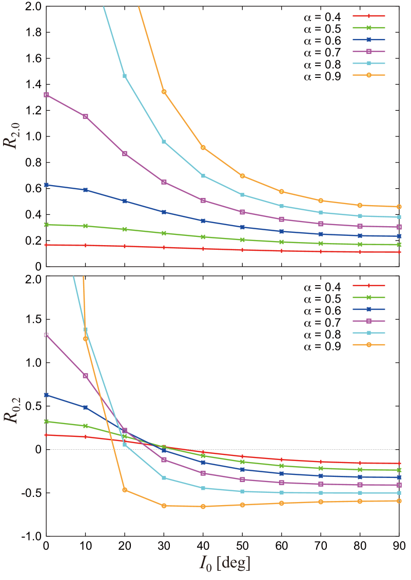
Figure 14: Dependence of the numerical values of $R_{2.0}$ (upper) and $R_{0.2}$ (lower) on $I_{0}=\cos^{-1}k$ and on $\alpha$. The plots are based on the values tabulated on an unnumbered table in von Zeipel (1910, pp. Z389–Z390).

Using the formulas (Z88-292), (Z89-294), (Z90-295), (Z(c)-296), (Z(d)-297), (Z(e)-298), von Zeipel calculates the actual numerical values of $R_{2.0}$ and $R_{0.2}$. He tabulated them on an unnumbered table on pp. Z389–Z390. The table shows the values of $R_{2.0}$ and $R_{0.2}$ having $I_{0}\left(=\cos^{-1}k\right)$ and $\alpha$ as parameters. The range of $I_{0}$ is from 0 to $90^{\circ}$ with an interval of $10^{\circ}$, and the range of $\alpha$ (or $a$ in von Zeipel’s notation) is from 0.4 and 0.9 with an interval of 0.1. Instead of just transcribing the table in this monograph, we make visual plots of their values in our Fig. 14.

Looking at the upper panel of Fig. 14, it is clear that $R_{2.0}>0$ is true everywhere in the given parameter range ($0.4\leq\alpha\leq 0.9$ and $0\leq I_{0}\leq\frac{\pi}{2}$). von Zeipel also gave a further guess about $R_{2.0}$:

“It is even likely that $R_{2.0}$ remains $>0$, whenever $0<\alpha\leq 1$.” (p. Z389)

Although von Zeipel placed the above statement here just as a conjecture without a rigorous proof, it seems that this conjecture is probably true. Indeed at each of the $I_{0}$ values, $R_{2.0}$ monotonically increases as $\alpha$ increases over the entire range of $I_{0}$. It is unlikely that $R_{2.0}$ becomes negative when $\alpha$ gets larger than 0.9. On the other hand when $\alpha$ becomes smaller than 0.4, the quadrupole level approximation $\left(\alpha^{2}\ll 1\right)$ would be applicable, and $R_{2.0}$ would remain positive according to Eq. (Z78-254).

In contrast to $R_{2.0}$, $R_{0.2}$ takes both positive and negative values (see the lower panel of Fig. 14). Let us cite von Zeipel’s description about the behavior of $R_{0.2}$:

“It also appears that the equation $R_{0.2}=0$ defines a function $k^{2}_{0.2}$ of $a$, increases with $a$ (at least as $a\leq 0.9$) and takes the value $k^{2}_{0.2}=+\frac{3}{5}$ for $a=0$, and probably the value $k^{2}_{0.2}=+1$ for $a=1$. We finally have $R_{0.2}>0$ when $k^{2}_{0.2}<k^{2}<1$, and $R_{0.2}<0$ when $0<k^{2}<k^{2}_{0.2}$.” (p. Z389)

By interpolating the numerical values of $R_{0.2}$, von Zeipel calculated the values of $I_{0.2}=\cos^{-1}k_{0.2}$ that realize $R_{0.2}=0$ at each $\alpha$. He tabulated them in an unnumbered table on p. Z389. Here, we should recall the fact that the origin $(x,y)=(\xi,\eta)=(0,0)$ changes its characteristics as a local extremum of $R$ according to the sign of $R_{0.2}$. This is obvious from the definition of $R_{2.0}$ and $R_{0.2}$ in Eqs. (Z77-253) and (Z78-254). From the development form in Eq. (Z77-253) this fact should remain true even when $\alpha$ is not so small. He then states a theorem as follows:

“The function $k_{0.2}$ being thus defined, we can state the following theorem:

At the origin $\xi=\eta=0$, the function $R$ has a minimum if $k^{2}_{0.2}<k^{2}<1$, and a saddle point if $0<k^{2}<k^{2}_{0.2}$.” (p. Z390)

In order to visually confirm von Zeipel’s result in comparison with modern knowledge, in Fig. 15 we plotted the values of $I_{0.2}$ that he tabulated as a function of $\alpha$. For comparison, in Fig. 15 we also plotted Kozai’s limiting inclination $i_{0}$ calculated through his numerical harmonic analysis (see the third column of Kozai’s Table I in p. K592, as well as Kozai’s Fig. 1 in p. K593. See also our Table 1 on p. 1 of this monograph). As we have learned, both von Zeipel’s $I_{0.2}$ and Kozai’s $i_{0}$ represent the threshold value of the perturbed body’s inclination whether or not the origin $(0,0)$ makes a saddle point. The comparison seen in Fig. 15 evidently tells us that von Zeipel’s $I_{0.2}$ almost exactly matches Kozai’s $i_{0}$ up to $\alpha=0.9$. This fact proves very well the correctness of von Zeipel’s theory and the calculation for the existence of local extremums in $R$ even when $\alpha$ is not small. Hence, the above theorem that von Zeipel states turns out not only qualitatively true but also quantitatively accurate.

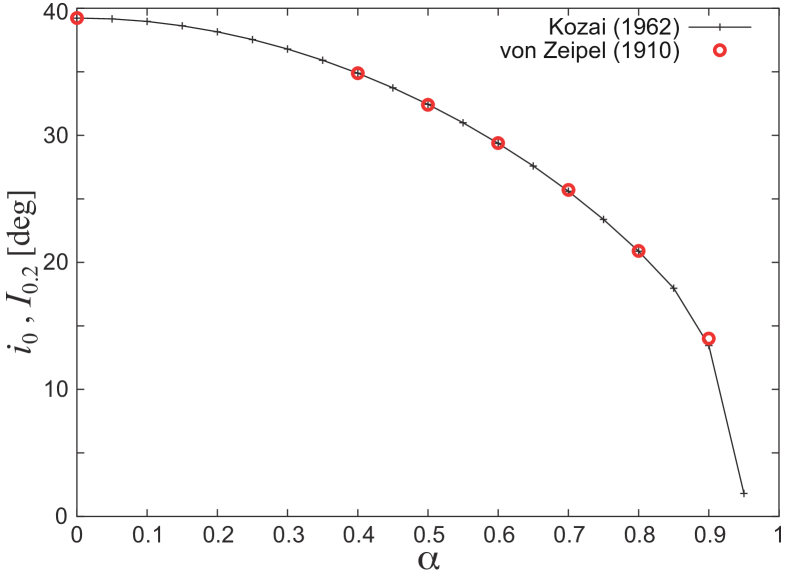
Figure 15: Dependence of von Zeipel’s $I_{0.2}$ and Kozai’s $i_{0}$ on $\alpha$. Red open circles denote the values of $I_{0.2}=\cos^{-1}k_{0.2}$ tabulated in von Zeipel (1910, p. Z399). Black lines with $+$ denote the numerically calculated values of $i_{0}$ in Kozai (1962, his Table I, the third column. It is transcribed in our Table 1 on p. 1 of this monograph).

Right after stating the above theorem, by recalling the result presented in his Section Z11 where he described the characteristics of the origin $(x,y)=(0,0)$ as a local extremum of $R$ (see our Section 5.4, in particular p. 5.4), von Zeipel states yet another theorem:

“By comparing this result to that of no. Z11, we can obviously express the theorem in question in the following way:

Suppose that the eccentricity of the orbit of an infinitely small mass located at the interior of the perturbing planet is small at a given moment; for this eccentricity to be always be small, it is necessary and sufficient that $I<I_{0.2}$.

In this statement we have neglected the perturbing mass and the square of the eccentricity.” (p. Z390)

Note that “no. Z11” in the above citation denotes von Zeipel’s Section Z11. We added the prefix Z for clarity. Similar expressions (such as “no. Z7” or “no. Z16”) appear several times in the remaining part of this monograph when we cite von Zeipel’s original descriptions.

Having von Zeipel’s previous theorem (p. 5.6.3) in mind, it is now obvious that his above theorem is true too. When $I>I_{0.2}$, the origin $(x,y)=(0,0)$ becomes a saddle point, and the perturbed body cannot always stay near the origin with a small eccentricity. The origin $(0,0)$ becomes a local minimum only when $I<I_{0.2}$, and the perturbed body can always stay near the origin with a small eccentricity if its initial eccentricity is small. The two circumstances were already depicted in von Zeipel’s schematic illustration that we transcribed before (Fig. 13 of this monograph).

Actual asteroids in the solar system

In Section Z18 von Zeipel tries to evaluate how large an asteroid’s eccentricity can increase when its inclination $I$ exceeds $I_{0.2}$. Although we do not go into the contents of Section Z18 in this monograph, readers with an interest might want to compare his discussion with modern analytic studies on a similar topic such as Kinoshita and Nakai (2007, their Eq. (31) on p. 71) and Antognini (2015, his Eqs. (28)–(30) on p. 3613). After that, in Section Z19 von Zeipel picks several asteroids that were actually recognized by his time from an ephemeris. He considers them as candidate objects that may have a large secular oscillation of eccentricity due to their large inclination. In what follows, we present a brief summary of the contents of his Section Z19.

As von Zeipel wrote (p. Z392), orbital elements of 665 asteroids are listed in Berliner Astronomisches Jahrbuch für 1911 (pp. (2)–(35)). Among them, he found that only six asteroids have $I_{0}$ that is larger than their $I_{0.2}$. They are (2) Pallas, (183) Istria, (473) Nolli, (531) Zerlina, (582) Olympia, and (594) Mireille. He points out a possibility that these asteroids have a secular variation of eccentricity with a large amplitude. Citing his words:

”Among the asteroids, in the number of 665, whose elements are in the Berliner Jahrbuch for the year 1911, there are only six whose quantity

$$I_{0}=\arccos\left(\sqrt{1-e^{2}}\cos I\right)$$

exceeds the limit $I_{0.2}$. Here are the planets in question

(2), (183), (473), (531), (582), (594).

We thus have

$$I_{0} =38^{\circ}.0 I_{0.2} =32^{\circ}.3$$ for (594)

$$I_{0} =36.7 I_{0.2} =31.5$$ for (2)

while for the other four planets, the difference $I_{0}-I_{0.2}$ is less considerable.

For the two planets (594) and (2), the amplitude of the secular perturbations of the eccentricity must be considerable.” (p. Z392)

For demonstrating and confirming von Zeipel’s prediction, we carried out a set of direct numerical integration of the orbit propagation of these six asteroids in the framework of CR3BP. Our numerical integration started from their orbital elements that had been published in Berliner Astronomisches Jahrbuch für 1911. We placed Jupiter on a circular orbit as the perturber. The numerical integration scheme, stepsize, and data output interval are all common to what was used to draw Fig. 8 (see p. 8 of this monograph for details). The total integration period is one million years, and the result is shown as Fig. 16. We summarized the parameters $k^{2}$, $\alpha$, and $c_{2}$ for the six asteroids in Table 2. In this table, $\alpha=\frac{a}{a^{\prime}}$ is the semimajor axes ratio between the asteroid and Jupiter. $c_{2}$ is what Lidov devised in Eq. (153).

As seen in Fig. 16, we can say that von Zeipel’s prediction “the amplitude of the secular perturbations of the eccentricity must be considerable” turns out to be largely correct, not only for (2) Pallas and (594) Mireille but also for the other four asteroids. Although the $k^{2}$ values are larger than the critical value $\left(k^{2}_{0.2}=\frac{3}{5}\right)$ of the quadrupole level approximation (see Table 2) for all the six asteroids, it seems that most of the asteroids probably possess stationary points on their disturbing potential along the axis of $g=\pm\frac{\pi}{2}$. This is because these asteroids have non-negligible $\alpha$ values, and we cannot simply apply the thresholds that are valid only at the quadrupole level approximation.

Incidentally, let us note that among the six asteroids that von Zeipel picked, two of them (Pallas and Zerlina) are now categorized in the Pallas family (e.g. Nesvorný, 2015). Mireille may be one of the Pallas family members too (e.g. Kozai, 1979, his Fig. 1). We believe that this is the reason why their orbital elements are close to each other.

von Zeipel also briefly mentions the status of “the comet Tempel” in this section as follows:

“Regarding the periodic comets, it must be mentioned that the quantity $I_{0}-I_{0.2}$ is generally $>0$. It is only the comet Tempel that is [an] exception. We have, in fact, for this comet

$$I_{0}=25^{\circ}.9\quad I_{0.2}=26^{\circ}.9.$$

” (p. Z392)

However currently, neither of the comets named “Tempel” has that large inclination: 9P/Tempel 1 has $I\sim 10^{\circ}.5$, and 10P/Tempel 2 has $I\sim 12^{\circ}.0$ (from the JPL Small-Body Database Search Engine). Therefore we do not go into the above statement any further.

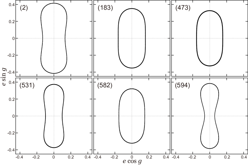
Figure 16: Numerically obtained trajectories of the six actual asteroids on the $(e\cos g,e\sin g)$ plane having Jupiter on a circular orbit as the perturber. Upper, from the left: (2) Pallas, (183) Istria, (473) Nolli. Lower, from the left: (531) Zerlina, (582) Olympia, (594) Mireille.

Table 2: Parameters $k^{2}$, $\alpha$, $c_{2}$ of the six asteroids that von Zeipel chose as examples in Section Z19. We calculated these values from the published orbital elements on Berliner Astronomisches Jahrbuch für 1911.

name	$k^{2}$	$\alpha$	$c_{2}$
(2) Pallas	0.6371525	0.532757	0.0116807
(183) Istria	0.7039341	0.536969	0.0250717
(473) Nolli	0.7316754	0.572902	0.0161331
(531) Zerlina	0.6540550	0.538855	0.0068172
(582) Olympia	0.7123067	0.503593	0.0126522
(594) Mireille	0.6207999	0.505205	0.0151757

Along the $y$-axis

Back to the search for local extremums of $R$, in Section Z20 von Zeipel focuses on demonstrating that $R$ possesses local minima at the two symmetric points $(x,y)=(0,\pm e_{0.2})$, even when $\alpha$ is not small. In this section, von Zeipel assumes $k^{2}$ is small. He does not give general demonstrations for arbitrary values of $k^{2}$, writing as follows at the beginning of this section:

“We have demonstrated at no. Z16 that the function $R$ possesses minimum values at the two symmetric points

$$x=0,\quad y=\pm e_{0.2}$$

if $a$ is small and if

$$R_{0.2}<0.$$ (Z92-300)

These minima, do they exist for any values of $a$ when the inequality (Z92) is satisfied?

I did not succeed in demonstrating it generally.

But I will now show that, [for] $a$ having any values, these minima on the axis of $y$ exist, if $k^{2}$ is small enough.” (pp. Z392–Z393)

von Zeipel’s mathematical demonstration presented in Section Z20 is rather brief and concise compared with those in other sections with extreme details. Formulas presented in Section Z20 show up mostly in their final form, and a large part of their derivations is omitted. In some part of what follows we try to complement what von Zeipel presented in this section. This is for facilitating the reader’s understanding of his original intention.

Section Z20 starts from the expression of the doubly averaged disturbing function $R$ using a single integral, rather than a double integral such as Eq. (Z44-224). von Zeipel already carried out a discussion on the characteristics of $R$ expressed as a single integral as Eq. (Z51-240) in Section Z14, Chapter III (p. Z47-235 of this monograph). Now, changing the integration variable in Eq. (Z51-240) from true anomaly $w$ to eccentric anomaly $u$, he formally expresses $R$ as

$$R=\frac{1}{2\pi a}\int^{2\pi}_{0}\frac{r}{\sqrt{1+r^{2}}}F(\tau)du.$$ (Z93-301)

Let us bear in mind that we are now searching local minima along the axis where $\cos 2g=-1$ is satisfied. Substituting $g=\pm\frac{\pi}{2}$ into Eq. (Z48-236), von Zeipel obtains an expression of $\tau$ (at $g=\pm\frac{\pi}{2}$) as follows

$$\tau^{2}=\frac{4r^{2}}{\left(1+r^{2}\right)^{2}}\left(\sin^{2}w+\cos^{2}I\cos^{2}w\right)$$ (303)

$$=\frac{4a^{2}}{\left(1+r^{2}\right)^{2}}\left[\left(1-e^{2}\right)\sin^{2}u+\frac{k^{2}}{1-e^{2}}\left(\cos u-e\right)^{2}\right].$$

Note that in Eqs. (Z93-301) and (303) we use $a$ instead of $\alpha$ due to the same formal reason as we stated on p. 12.

Here, von Zeipel assumes that $k$ is a small quantity of the first-order. Then he introduces a finite, non-zero, non-dimensional variable $\rho$ as follows:

$$1-e^{2}=\rho k,$$ (304)

which is equivalent to

$$e=\sqrt{1-\rho k}.$$ (305)

Now von Zeipel states that $\tau^{2}$ at $g=\pm\frac{\pi}{2}$ in Eq. (303) is a small quantity of the first-order. This is true because $k^{2}$ is a small quantity of the second-order from his assumption here, and $1-e^{2}$ is a small quantity of the first-order due to Eq. (304). Then, using Eq. (305) von Zeipel expands $\tau^{2}$ at $g=\pm\frac{\pi}{2}$ into the series of $k$ as follows (p. Z393):

$$\tau^{2}=4\alpha^{2}\Phi^{2}\left[\rho\sin^{2}u+\frac{\left(\cos u-1\right)^{2}}{\rho}\right]k+\cdots,$$ (306)

where $\Phi$ is a function of $u$ defined as

$$\Phi=\frac{1}{1+\alpha^{2}(1-\cos u)^{2}}.$$ (307)

Note that in Eqs. (306) and (307) we use $\alpha$ instead of $a$ for formal consistency, as $\Phi$ seems non-dimensional in von Zeipel’s discussion in Section Z20.

Adopting Eqs. (306) and (307) to Eq. (Z93-301), von Zeipel shows an expanded form of $R$ in the series of $k$ at $g=\pm\frac{\pi}{2}$ as follows:

$$R=R_{0}+\left(P\rho+Q\frac{1}{\rho}\right)k+\cdots,$$ (308)

where

$$R_{0}=\frac{1}{2\pi}\int_{0}^{2\pi}\Phi^{\frac{1}{2}}\left(1-\cos u\right)du,$$ (309)

$$P =\frac{1}{4\pi}\int_{0}^{2\pi}\Phi^{\frac{3}{2}}\cos udu$$ (310)

$$\quad+\frac{3\alpha^{2}}{8\pi}\int_{0}^{2\pi}\Phi^{\frac{5}{2}}\sin^{2}u\left(1-\cos u\right)du,$$

$$Q=\frac{3\alpha^{2}}{8\pi}\int_{0}^{2\pi}\Phi^{\frac{5}{2}}\left(1-\cos u\right)^{3}du.$$ (311)

At this point, von Zeipel claims that $P$ defined in Eq. (310) and $Q$ defined in Eq. (311) are both positive. Let us cite what von Zeipel wrote:

“$Q$ is a positive quantity. In the expression of $P$, the second term is obviously positive. The first term is also positive because the quantity $\Phi$ decreases with $\cos u$. We therefore have $P>0$, $Q>0$.” (p. Z394)

The fact that both $P$ and $Q$ are positive turns out to be important later. But we think that his above statement “We therefore have $P>0$, $Q>0$” needs more confirmation and clarification. For this purpose, we have made a little more exposition and put it in Appendix A.

Now, von Zeipel moves on to a consideration of a solution of the following equation

$$\left.\frac{\partial R}{\partial e}\right|_{g=\pm\frac{\pi}{2}}=0.$$ (312)

Using the relationship (304) between $e$ and $\rho$ together with the expression of $R$ in Eq. (308), he deforms the equation (312) as (p. Z394):

$$-2\left(P-\frac{Q}{\rho^{2}}\right)+A_{1}k+A_{2}k^{2}+\cdots=0,$$ (313)

where $A_{1}$, $A_{2}$, $\cdots$ are polynomials of $\rho$ or $\rho^{-1}$ whose actual form he did not show. Right after stating Eq. (313), von Zeipel tries to obtain the solution of Eq. (312). He writes:

“It [Eq. (313)] has a positive root developed in powers of $k$, and being reduced to $\sqrt{Q:P}$, when $k=0$.

As a result, the equations

$$\frac{\partial R}{\partial e}=0,\quad\frac{\partial R}{\partial g}=0$$

are satisfied by putting

$$g =\pm\frac{\pi}{2},$$ (Z94-313)

$$e =e_{0.2}$$

$$=1-\frac{1}{2}\sqrt{\frac{Q}{P}}\cdot k+E_{2}k^{2}+E_{3}k^{3}+\cdots.$$

The semi-major axis $a$ being fixed arbitrarily, the series giving $e_{0.2}$ converges if $k$ is small enough.” (p. Z394)

Here we see that the solution of Eq. (313), $\rho=\sqrt{Q:P}$ $\bigl{(}=\sqrt{Q/P}\bigr{)}$, can exist as a real number owing to the fact that both $P$ and $Q$ are positive, as previously shown. Note that the second equation in (Z94-313) is a Taylor-series expansion of the eccentricity $e$ by $k$ using the relationship (305). See its similarity to, and difference from, Eq. (Z81-269) in the $\alpha\ll 1$ approximation. Note also that $E_{2}$, $E_{3}$, $\cdots$ in Eq. (Z94-313) must be polynomials of $P$ and $Q$, although von Zeipel does not mention anything about them.

Now, von Zeipel moves on to a calculation of the second derivatives of $R$ at the points $(e,g)=(e_{0.2},\pm\frac{\pi}{2})$, and tries to show that these points are local minima of $R$ when $k$ is small. From the definition of $\rho$ in Eq. (304), at these points (where $\rho=\sqrt{Q/P}$) he obtains a relation (p. Z394):

$$\frac{\partial^{2}R}{\partial e{}^{2}} =-\frac{2}{k}\frac{\partial R}{\partial\rho}+\frac{4e^{2}}{k^{2}}\frac{\partial^{2}R}{\partial\rho{}^{2}}$$ (315)

$$=\frac{4}{k}\frac{2Q}{\rho^{3}}+\cdots$$

$$=\frac{8P}{k}\sqrt{\frac{P}{Q}}+\cdots>0.$$

Note that in the second line of Eq. (315), the first term is at the order of $O\left(k^{-1}\right)$, and the remaining terms (specifically writing, $-\frac{6Q}{\rho^{2}}-2P+\cdots$) are at the order of $O\left(k^{0}\right)$.

von Zeipel also claims that (p. Z394)

$$\frac{\partial^{2}R}{\partial e\partial g}=0,$$ (316)

which is true from the general definition of $R$ in Eq. (Z72-246) when $g=\pm\frac{\pi}{2}$.

Then from Eqs. (Z48-236) and (Z93-301), he calculates the following quantity at $g=\pm\frac{\pi}{2}$ (pp. Z393–Z394):

$$\frac{\partial^{2}R}{\partial g{}^{2}}= \frac{1}{2\pi}\int_{0}^{2\pi}\frac{r}{a}\frac{1}{\sqrt{1+r^{2}}}\frac{8\sin^{2}I}{\left(1+r^{2}\right)^{2}}$$ (317)

$$\times \left(\frac{\partial F}{\partial\left(\tau^{2}\right)}r^{2}-2\frac{\partial F}{\partial\left(\tau^{2}\right)}r^{2}\sin^{2}w\right.$$

$$\left.+\frac{\partial^{2}F}{\partial\left(\tau^{2}\right){}^{2}}\frac{8\sin^{2}I}{\left(1+r^{2}\right)^{2}}r^{2}\sin^{2}w\cdot r^{2}\cos^{2}w\right)du.$$

Note that the dimension of $\tau^{2}$ is that of $r^{-2}$ from Eq. (303). This guarantees the consistency of the dimensions of the left- and right-hand sides of Eq. (317)

Next, von Zeipel expands $\frac{\partial^{2}R}{\partial g{}^{2}}$ into a power series of $k$ by applying the following relationship between eccentric anomaly and true anomaly to Eq. (317):

$$r^{2}\sin^{2}w =a^{2}\left(1-e^{2}\right)\sin^{2}u,$$ (318)

$$r^{2}\cos^{2}w =a^{2}\left(\cos u-e\right)^{2}.$$ (319)

Note that in Eqs. (317), (318) and (319), we use $a$ instead of $\alpha$ due to the same formal reason as mentioned before (see p. 12 and p. 303 of this monograph).

Among the expanded terms, von Zeipel picks only those that are independent of $k$. He eventually shows an inequality

$$\frac{\partial^{2}R}{\partial g{}^{2}}=2Q+\cdots>0.$$ (320)

The signs of the second derivatives of $R$ presented as Eqs. (315), (316), and (320) tell us that the points $(e,g)=(e_{0.2},\pm\frac{\pi}{2})$ are local minima of $R$ for arbitrary values of $\alpha$ as long as $k$ is small. Here von Zeipel makes a statement on the equivalence of the expansion of $e_{0.2}$ in Eq. (Z94-313) to that in Eq. (Z81-269) when $\alpha$ is small, although no rigorous demonstration is given:

“For small values of $\alpha$, the quantity $e_{0.2}$ of the formula (Z94) can obviously be expanded in powers of $\alpha^{2}$. The development thus obtained coincides with that given by the equation (Z81). Indeed, we have seen in no. Z16, that such formula (Z81) gives all the minima of the function $R$ when $\alpha$ and $k$ are small.” (p. Z395)

As we learned in von Zeipel’s Chapters II and III, the existence of a local minimum on the equi-potential surface indicates a possibility to construct the Lindstedt series around it. von Zeipel mentions the characteristics of the perturbed body’s orbit around the local minimum at $(e,g)=(e_{0.2},\pm\frac{\pi}{2})$. We literary cite his words:

“We can apply the results of this issue by calculating, according to no. Z10, the Lindstedt series, which exists when the elements are in the vicinity of the points (Z94). The corresponding orbits belong to a certain class of comets in a stable motion. In these orbits, the semimajor axis is arbitrary; the eccentricity is close to unity; the distance from the perihelion to the node is close to $\pm\frac{\pi}{2}$; the inclination is considerable; Finally, the parameter $a\left(1-e^{2}\right)$ is small, so that the two nodes are located inside the orbit of Jupiter.” (p. Z395)

Note that in the above, “the parameter $a\left(1-e^{2}\right)$” denotes the semilatus rectum $\ell$ of the perturbed body. von Zeipel’s above statement depicts the dynamical characteristics of “a certain class of comets in a stable motion” trapped around one of the stationary points, $(e,g)=(e_{0.2},\pm\frac{\pi}{2})$.

The next section (Z21) is devoted to describing the dynamical characteristics of an example object that has such an orbit described above: The comet 1P/Halley whose $a\sim 18$ au and $\ell\sim 1.15$ au (these values are due to von Zeipel). However, we do not go into this subject right now. Instead, we will return to it later again (Section 5.8.1 on p. 5.8.1 of this monograph) after we have reviewed the case when $\alpha>1$ (Sections Z22–Z23) and the case when the orbits of the perturbed and perturbing bodies intersect (Sections Z24–Z25). This is mainly because 1P/Halley satisfies the condition $\alpha>1$ with respect to the most massive perturbing planet, Jupiter. In this regard, we wonder why von Zeipel brought up the subject on the motion of 1P/Halley in a section that discusses the inner CR3BP where $\alpha<1$.

5.7 Secular disturbing function: Outer case

One of the biggest differences between von Zeipel’s work and those of Lidov or Kozai is that, von Zeipel dealt with the so-called outer version of the doubly averaged CR3BP in his 1910 publication. We would dare to say that detailed studies of the outer CR3BP did not seriously begin until the 1990s when the actual “outer” objects were recognized in the solar system, such as the transneptunian objects (TNOs) perturbed by Neptune (e.g. Jewitt and Luu, 1993; Jewitt, 1999; Thomas and Morbidelli, 1996; Lykawka, 2012). Therefore the relevant publications are much fewer than those on the inner CR3BP. In his Sections Z22 and Z23, von Zeipel focuses on describing the basic theoretical framework of the doubly averaged outer CR3BP with particular emphasis on the search for local extremums of the secular disturbing function. Calculations for locating local extremums of the doubly averaged disturbing function for the outer CR3BP is substantially more complicated than those for the inner CR3BP, as we will see in what follows.

5.7.1 Expansion of $R$ by $\alpha^{\prime}$

Similar to the inner problem that we described in Section 5.6 (p. 5.6 of this monograph), von Zeipel’s treatment of the doubly averaged outer CR3BP begins with an expansion of the disturbing function with respect to the ratio of semimajor axis of the perturbed and perturbing bodies. Now the variable for the expansion is $\alpha^{\prime}=\frac{a^{\prime}}{a}$, which is smaller than 1.

As for the expansion using $\alpha^{\prime}$, von Zeipel again follows what Tisserand (1889) did with the Hansen coefficients. The resulting expansion form is as follows:

$$R =\sum_{m=1}^{\infty}\Bigl{(}A_{0.0}^{(2m)}X_{0}^{-(2m+1),0}$$ (Z96-320)

$$\quad+2\sum_{i=1}^{m}A_{i.i}^{(2m)}X_{0}^{-(2m+1),2i}\cos 2ig\Bigr{)}{\alpha^{\prime}}^{2m+1},$$

where

$$X_{0}^{-(2m+1),2i}$$ (Z95-321)

$$=\frac{(2m-1)!}{(2m-2i-1)!(2i)!}\left(\frac{e^{2}}{4}\right)^{i}\left(1-e^{2}\right)^{-2m+\frac{1}{2}}$$

$$\quad\times F\left(i-m+1,i-m+\frac{1}{2},2i+1,e^{2}\right),$$

are the Hansen coefficients. $k_{i,j}^{(2m)}$ and $A_{i,j}^{(2m)}$ are already defined in Eqs. (Z73-249) and (Z74-248).

Then von Zeipel rewrites the expansion of $R$ in Eq. (Z96-320) as follows:

$$R=R^{\prime}_{3}{\alpha^{\prime}}^{3}+R^{\prime}_{5}{\alpha^{\prime}}^{5}+\cdots,$$ (Z97-322)

where

$$R^{\prime}_{3} =A_{0.0}^{(2)}X_{0}^{-3,0}$$ (Z98-323)

$$=\frac{1}{4}\left(1-\frac{3}{2}\sin^{2}I\right)\left(1-e^{2}\right)^{-2+\frac{1}{2}},$$

$$R^{\prime}_{5} =A_{0.0}^{(4)}X_{0}^{-5,0}+2A_{1.1}^{(4)}X_{0}^{-5,2}\cos 2g$$

$$=\frac{9}{64}\left[\left(1-5\sin^{2}I+\frac{35}{8}\sin^{4}I\right)\left(1+\frac{3}{2}e^{2}\right)\right.$$

$$\left.+\frac{15}{4}\sin^{2}I\left(1-\frac{7}{6}\sin^{2}I\right)e^{2}\cos 2g\right]\left(1-e^{2}\right)^{-4+\frac{1}{2}}.$$

In Eqs. (Z97-322) and (Z98-323), we should notice that $R$’s leading term $(R^{\prime}_{3})$ does not depend on $g$. The $g$-dependence of $R$ first shows up in the next order term $(R^{\prime}_{5})$. This is a stark difference from the inner problem, and it makes the secular perturbation in the outer CR3BP subtler than in the inner problem (e.g. Ito, 2016). Note also that in the expression of $R$ in Eq. (Z97-322), the lowest-order term is of the order of $O\bigl{(}{\alpha^{\prime}}^{3}\bigr{)}$, not $O\bigl{(}{\alpha^{\prime}}^{2}\bigr{)}$. Compare Eq. (Z97-322) with the corresponding expansions in the inner problem (Eq. (Z75-250)) where the lowest-order term is at the order of $O\left(\alpha^{2}\right)$ except for a constant. This is another factor that makes the secular perturbation in the outer CR3BP weaker than in the inner problem.

In von Zeipel’s original paper, he uses $a^{\prime}$ instead of $\alpha^{\prime}=\frac{a^{\prime}}{a}$ throughout the discussion on the outer problem. He poses an unnumbered equation on p. Z397 as

$$a^{\prime}=\frac{1}{a}.$$ (325)

The numerator $(1)$ in Eq. (325) denotes the value of the semimajor axis of the perturber (Jupiter). Hence, his original form of Eq. (Z97-322) is as follows:

$$R=R^{\prime}_{3}{a^{\prime}}^{3}+R^{\prime}_{5}{a^{\prime}}^{5}+\cdots.$$ (326)

However, we think that the use of $a^{\prime}$ defined by Eq. (325) is very confusing for the readers of this monograph, because we have basically used $a^{\prime}$ as the semimajor axis of the perturbing body. For avoiding the confusion, and maintaining compatibility with the descriptions in the previous sections, in what follows we use the variable $\alpha^{\prime}$ instead of von Zeipel’s $a^{\prime}$. We also need to be aware that in Eq. (326) (therefore in Eq. (Z97-322)) von Zeipel uses the notation $R$ for the doubly averaged disturbing function without adding a superscript dash. Only its expanded components on the right-hand side $\left(R^{\prime}_{3},R^{\prime}_{5},\cdots\right)$ have a superscript dash.

Similar to the discussion on the inner problem (see p. Z97-322), von Zeipel next expands $R$ of Eq. (Z97-322) into a two-variable Taylor series using the variables $x^{2}=e^{2}\cos^{2}g$ and $y^{2}=e^{2}\sin^{2}g$ as follows:

$$R=R^{\prime}_{0.0}+R^{\prime}_{2.0}x^{2}+R^{\prime}_{0.2}y^{2}+\cdots.$$ (Z99-326)

The coefficients $R^{\prime}_{2.0}$ and $R^{\prime}_{0.2}$ themselves are expanded into a power series of $\alpha^{\prime}$ as

$$R^{\prime}_{2.0} =-\frac{3}{16}\left(1-5k^{2}\right){\alpha^{\prime}}^{3}$$ (Z100-327)

$$+ \frac{45}{256}\left(1-14k^{2}+21k^{4}\right){\alpha^{\prime}}^{5}+P^{\prime}_{7}{\alpha^{\prime}}^{7}+\cdots,$$

$$R^{\prime}_{0.2} =-\frac{3}{16}\left(1-5k^{2}\right){\alpha^{\prime}}^{3}$$

$$+ \frac{45}{256}\left(2-22k^{2}+28k^{4}\right){\alpha^{\prime}}^{5}+Q^{\prime}_{7}{\alpha^{\prime}}^{7}+\cdots,$$

where $P^{\prime}_{2i+1}$ and $Q^{\prime}_{2i+1}$ are certain polynomials in $k^{2}$, although von Zeipel did not give their actual forms.

von Zeipel did not show the specific form of the first term in Eq. (Z99-326), $R^{\prime}_{0.0}$. But we can calculate it by carrying out the two-variable Taylor expansion. The result is:

$$R^{\prime}_{0.0}=-\frac{1-3k^{2}}{8}{\alpha^{\prime}}^{3}+\frac{27-270k^{2}+315k^{4}}{512}{\alpha^{\prime}}^{5}+\cdots.$$ (329)

However, similar to the inner case (Eq. (256) on p. 256), constant terms such as $R^{\prime}_{0.0}$ do not matter in the following discussions. This is because von Zeipel’s major concern was to search for local extremums of $R$ by calculating its partial derivatives. Constant terms such as $R^{\prime}_{0.0}$ in the disturbing function will be all gone by the differentiation.

5.7.2 Search of local extremums

In the rest of Section Z22, von Zeipel tries to locate local extremums of $R$ in Eq. (Z99-326). The logical structure of this part is the same as in Section Z16 (see p. 5.6.2 of this monograph). He picks several possible regions where $R$ can take local extremums: At the origin, on the outer boundary, and along the $y$- and $x$-axis on the $(x,y)=(e\cos g,e\sin g)$ plane. Then he moves on to checking out the type of the local extremums that he discovered in these regions. Following von Zeipel, in this subsection we assume $\alpha^{\prime}\ll 1$,

Similar to the discussion on the inner problem, von Zeipel begins with obtaining the solution of the pair of equations

$$R^{\prime}_{2.0} =0,$$ (330)

$$R^{\prime}_{0.2} =0.$$ (331)

In the inner problem where we have Eqs. (Z78-254) and (257), we learned that only $R_{0.2}$ can be zero, but $R_{2.0}$ cannot. On the other hand in the outer case, we will see that both $R^{\prime}_{2.0}$ and $R^{\prime}_{0.2}$ can be zero. This fact makes the outer problem more complicated than the inner problem.

von Zeipel denotes the root of Eq. (330) as ${k^{\prime}}^{2}_{2.0}$, and the root of Eq. (331) as ${k^{\prime}}^{2}_{0.2}$. Then, using Eq. (Z100-327) he expands ${k^{\prime}}^{2}_{2.0}$ and ${k^{\prime}}^{2}_{0.2}$ up to $O\bigl{(}{\alpha^{\prime}}^{2}\bigr{)}$ as

$${k^{\prime}}^{2}_{2.0} =\frac{1}{5}+\frac{9}{50}{\alpha^{\prime}}^{2}+\cdots,$$ (Z101-331)

$${k^{\prime}}^{2}_{0.2} =\frac{1}{5}+\frac{12}{50}{\alpha^{\prime}}^{2}+\cdots.$$

It is obvious that both ${k^{\prime}}^{2}_{2.0}$ and ${k^{\prime}}^{2}_{0.2}$ would approach $\frac{1}{5}$ in the limit of $\alpha^{\prime}\to 0$. Also, we see that

$${k^{\prime}}^{2}_{2.0}<{k^{\prime}}^{2}_{0.2},$$ (333)

although the difference is not large when $\alpha^{\prime}$ is small.

At the origin

The equations (Z99-326), (Z100-327), and (Z101-331) tell us the following fact as long as ${\alpha^{\prime}}^{2}\ll 1$:

$$R^{\prime}_{2.0}\lessgtr 0 \iff k^{2}\lessgtr{k^{\prime}}^{2}_{2.0},$$ (334)

$$R^{\prime}_{0.2}\lessgtr 0 \iff k^{2}\lessgtr{k^{\prime}}^{2}_{0.2}.$$ (335)

Combining the facts of (334), (335), and (333), von Zeipel claims that the doubly averaged disturbing function $R$ in Eq. (Z99-326) has a local extremum around the origin $(x,y)=(0,0)$. He also mentions that the origin $(0,0)$ has the following characteristics as long as $\alpha^{\prime}\ll 1$ (p. Z399):

• $(0,0)$ is a local minimum when ${k^{\prime}}^{2}_{0.2}<k^{2}<1$,

• $(0,0)$ is a saddle point when ${k^{\prime}}^{2}_{2.0}<k^{2}<{k^{\prime}}^{2}_{0.2}$,

• $(0,0)$ is a local maximum when $0\leq k^{2}<{k^{\prime}}^{2}_{2.0}$.

We can accept these conclusions without any doubt because of the expansion form shown in Eq. (Z99-326).

At the outer boundary

von Zeipel then moves on to a consideration of $R$ on its outer boundary, $e=k^{\prime}$. In the inner problem, the boundary circle is a kind of a local maximum of $R$ (see p. 5.6.2). Similarly, by calculating the partial derivative $\frac{\partial R}{\partial(e^{2})}$ and substituting $e^{2}={k^{\prime}}^{2}=1-k^{2}$ into it, on the boundary circle he obtains for the outer case (p. Z399)

$$\left.\frac{\partial R}{\partial\left(e^{2}\right)}\right|_{e^{2}={k^{\prime}}^{2}} = \left.\frac{\partial R^{\prime}_{3}}{\partial\left(e^{2}\right)}\right|_{e^{2}={k^{\prime}}^{2}}{\alpha^{\prime}}^{3}+\cdots$$ (336)

$$= \frac{3}{4}\left(k^{2}\right)^{-\frac{5}{2}}{\alpha^{\prime}}^{3}+\cdots>0.$$

As long as $\alpha^{\prime}$ is so small that we can ignore the higher-order terms of $\alpha^{\prime}$, the right-hand side of Eq. (336) is always positive. Hence $\frac{\partial R}{\partial(e^{2})}>0$ is true on the outer boundary. This indicates that, just inside the outer boundary, $R$ continues to increase along the radial direction on the $(e\cos g,e\sin g)$ plane until it reaches $e=k^{\prime}$. In this sense, the outer boundary $x^{2}+y^{2}={k^{\prime}}^{2}$ can be regarded as a kind of local maximum of $R$, similar to the inner case.

Along the $y$-axis and $x$-axis

Next, von Zeipel moves on to search for $R$’s local extremums that may be located somewhere between the origin $(x,y)=(0,0)$ and the outer boundary $\bigl{(}x^{2}+y^{2}={k^{\prime}}^{2}\bigr{)}$. Similar to the discussion on the inner case (see p. 5.6.2), it is necessary to find solutions that satisfy both of the following equations

$$\frac{\partial R}{\partial\left(e^{2}\right)}=0,\quad\frac{\partial R}{\partial g}=0,$$ (Z102-336)

which is exactly the same as Eq. (Z80-266).

It is obvious that the operation $\frac{\partial R}{\partial g}$ eliminates the entire $R^{\prime}_{3}$ and the first term of $R^{\prime}_{5}$ in Eq. (Z98-323), and just leaves the second term of $R^{\prime}_{5}$. The second term of $R^{\prime}_{5}$ in Eq. (Z98-323) yields a factor of $\sin 2g$ through the operation $\frac{\partial R}{\partial g}$, so the roots of the equation $\frac{\partial R}{\partial g}=0$ in Eq. (Z102-336) take place when $\sin 2g=0$. This means $\cos 2g=+1$ or $-1$.

From the function form of $R$ in Eqs. (Z96-320) and (Z98-323), $\frac{\partial R}{\partial\left(e^{2}\right)}$ becomes as follows when $\cos 2g=+1$:

$$\frac{\partial R}{\partial\left(e^{2}\right)}={\alpha^{\prime}}^{3}\frac{3}{16}\left(1-e^{2}\right)^{-\frac{7}{2}}\left(-1+5k^{2}+e^{2}\right)$$

$$\quad-{\alpha^{\prime}}^{5}\frac{45\left(1-e^{2}\right)^{-\frac{13}{2}}}{2048}\left(-8+112k^{2}-168k^{4}+17e^{2}\right.$$

$$\quad\quad\left.-98e^{2}k^{2}-63e^{2}k^{4}-10e^{4}-14e^{4}k^{2}+e^{6}\right).$$ (338)

When $\cos 2g=-1$, $\frac{\partial R}{\partial\left(e^{2}\right)}$ becomes as:

$$\frac{\partial R}{\partial\left(e^{2}\right)}={\alpha^{\prime}}^{3}\frac{3}{16}\left(1-e^{2}\right)^{-\frac{7}{2}}\left(-1+5k^{2}+e^{2}\right)$$

$$\quad+{\alpha^{\prime}}^{5}\frac{45\left(1-e^{2}\right)^{-\frac{13}{2}}}{2048}\left(16-176k^{2}+224k^{4}-13e^{2}\right.$$

$$\quad\quad\left.-62e^{2}k^{2}+315e^{2}k^{4}-22e^{4}+238e^{4}k^{2}+19e^{6}\right).$$ (339)

Note that von Zeipel’s original equation (an unnumbered one on p. Z399) that corresponds to Eqs. (338) and (339) is truncated at the order of ${\alpha^{\prime}}^{3}$. Only the first terms in the right-hand side of Eqs. (338) and (339) are presented as:

$$\frac{\partial R}{\partial\left(e^{2}\right)} ={a^{\prime}}^{3}\frac{\partial R^{\prime}_{3}}{\partial\left(e^{2}\right)}+\cdots$$

$$={a^{\prime}}^{3}\frac{3}{16}\left(1-e^{2}\right)^{-\frac{7}{2}}\left(-1+5k^{2}+e^{2}\right)+\cdots.$$ (340)

Note also that we have ourselves calculated and added the terms of $O\bigl{(}{\alpha^{\prime}}^{5}\bigr{)}$ to this equation (we do not show their specific forms here), and then derived Eqs. (338) and (339). It is because the higher-order terms of $\alpha^{\prime}$ are necessary for obtaining the expressions of $e^{\prime}_{2.0}$ and $e^{\prime}_{0.2}$ in what follows.

Next, von Zeipel expresses the solution of the equation $\frac{\partial R}{\partial\left(e^{2}\right)}=0$. When $\cos 2g=+1$, it becomes:

$$e^{2} ={e^{\prime}}^{2}_{2.0}$$

$$=1-5k^{2}+\frac{3}{100}\frac{7-5k^{2}}{k^{2}}{\alpha^{\prime}}^{2}+\cdots.$$ (Z103-340)

When $\cos 2g=-1$, it becomes as follows:

$$e^{2} ={e^{\prime}}^{2}_{0.2}$$

$$=1-5k^{2}+\frac{3}{200}\frac{41-125k^{2}}{k^{2}}{\alpha^{\prime}}^{2}+\cdots.$$ (Z104-341)

Similar to the consideration in the inner case (see p. Z81-269), von Zeipel then proposes the equation

$${e^{\prime}}^{2}_{2.0}=0,$$ (343)

for the case of $\cos 2g=+1$ (equivalent to $g=0$ or $\pi$). Although he does not show the function form of $k^{2}$ that satisfies Eq. (343), we can calculate the form as

$$k^{2}=\frac{1}{5}+\frac{9}{50}{\alpha^{\prime}}^{2}+\cdots\equiv\overline{k^{\prime}_{2.0}}^{2}.$$ (344)

Equation (344) means that, when the value of $k^{2}$ approaches $\overline{k^{\prime}_{2.0}}^{2}$, both the two solutions $(e,g)=(e^{\prime}_{2.0},0)$ and $(e^{\prime}_{2.0},\pi)$ of the equation

$$\left.\frac{\partial R}{\partial\left(e^{2}\right)}\right|_{\cos 2g=+1}=0,$$ (345)

would approach the origin at $e=0$. In other words, the two solutions $(x,y)=(\pm e^{\prime}_{2.0},0)$ on the $(e\cos g,e\sin g)$ plane would approach $(x,y)=(0,0)$. We have already seen the behavior of $R$ at the origin $(0,0)$ on p. 5.7.2.

Note that von Zeipel uses the notation $\overline{k^{2}}$ (p. Z400) for expressing the solution of Eq. (343). However, we prefer to use $\overline{k^{\prime}_{2.0}}^{2}$ in this monograph. This is for distinguishing this quantity from a similar one that shows up in the following discussion on $e^{\prime}_{0.2}$ (see the descriptions around Eqs. (347) and (348)). It is also for maintaining a consistency with the discussion on the inner problem (see p. 272).

At this point, von Zeipel mentions the equivalence of ${k^{\prime}}^{2}_{2.0}$ in Eq. (Z101-331) and $\overline{k^{\prime}_{2.0}}^{2}$ in Eq. (344). Let us cite what he says. Note that in the quoted part below, we use his original notation $\overline{k^{2}}$, instead of our own $\overline{k^{\prime}_{2.0}}^{2}$:

“The quantity ${e^{\prime}}^{2}_{2.0}$ is not always positive. Indeed, it vanishes for a certain value of $k^{2}$ adjacent to $\frac{1}{5}$. Now let $\overline{k^{2}}$ [be] a root of the equation ${e^{\prime}}^{2}_{2.0}=0$. I say that $\overline{k^{2}}$ inevitably coincides with the quantity ${k^{\prime}}^{2}_{2.0}$, which cancels the coefficient $R^{\prime}_{2.0}$. Indeed, when $k^{2}$ passes the value $\overline{k^{2}}$, the two solutions

$$x=\pm e^{\prime}_{2.0},\quad y=0$$

of equations

$$\frac{\partial R}{\partial x}=\frac{\partial R}{\partial y}=0$$

coincide with the solution already studied

$$x=y=0.$$

It is therefore necessary that $\overline{k^{2}}$ cancels the coefficient $R^{\prime}_{2.0}$ and that, as a result, $\overline{k^{2}}$ coincides with the quantity ${k^{\prime}}^{2}_{2.0}$, given by the first [equation] of formulas (Z101).” (p. Z400)

von Zeipel’s statement above and Eq. (344) thus tell us that $\overline{k^{2}}$ (or $\overline{k^{\prime}_{2.0}}^{2}$ in our notation) is a key parameter for confirming or denying the existence of local extremums of $R$ on the $x$-axis of the $(e\cos g,e\sin g)$ plane.

Next he moves on to another, similar equation

$${e^{\prime}}^{2}_{0.2}=0,$$ (346)

for the case of $\cos 2g=-1$ (equivalent to $g=\pm\frac{\pi}{2}$). This equation corresponds to Eq. (271) in the discussion on the inner problem (see p. 271 of this monograph). Although von Zeipel does not show the function form of $k^{2}$ that satisfies Eq. (346), we can again calculate the form as

$$k^{2}=\frac{1}{5}+\frac{12}{50}{\alpha^{\prime}}^{2}+\cdots\equiv\overline{k^{\prime}_{0.2}}^{2}.$$ (347)

Equation (347) means that, when $k^{2}$ approaches $\overline{k^{\prime}_{0.2}}^{2}$, both the solutions $(e,g)=({e^{\prime}}^{2}_{2.0},\pm\frac{\pi}{2})$ of the equation

$$\left.\frac{\partial R}{\partial\left(e^{2}\right)}\right|_{\cos 2g=-1}=0,$$ (348)

approach the origin $e=0$. In other words, the two solutions $(x,y)=(0,\pm e^{\prime}_{0.2})$ on the $(e\cos g,e\sin g)$ plane would approach $(x,y)=(0,0)$. In addition, we can deduce the equivalence of ${k^{\prime}}^{2}_{0.2}$ in Eq. (Z101-331) and $\overline{k^{\prime}_{0.2}}^{2}$ in Eq. (347) due to the same reason as in the case of $\cos 2g=+1$. Somehow, however, von Zeipel’s statement about it is very short:

“In the same manner it is demonstrated that the quantity ${k^{\prime}}^{2}_{0.2}$, given by the second of the formulas (Z101), is the only root of the equation

$${e^{\prime}}^{2}_{0.2}=0.$$

It remains for us to examine whether the function $R$ is [a] maximum, minimum or minimaxima at the points (Z103) and (Z104).” (p. Z400)

von Zeipel’s above statement and Eq. (347) thus tell us that $\overline{k^{\prime}_{0.2}}^{2}$ is a key value for confirming (or denying) the existence of local extremums of $R$ on the $y$-axis of the $(x,y)=(e\cos g,e\sin g)$ plane.

As a summary, let us itemize the conclusions that von Zeipel obtained as follows:

• When $k^{2}<{k^{\prime}}^{2}_{2.0}$, ${e^{\prime}}^{2}_{2.0}$ becomes positive, and $R$ has two local extremums at $(x,y)=(\pm e^{\prime}_{2.0},0)$.

• When $k^{2}<{k^{\prime}}^{2}_{0.2}$, ${e^{\prime}}^{2}_{0.2}$ becomes positive, and $R$ has two local extremums at $(x,y)=(0,\pm e^{\prime}_{0.2})$.

• If $\alpha^{\prime}$ is small, we have ${k^{\prime}}^{2}_{2.0}<{k^{\prime}}^{2}_{0.2}$ from Eq. (Z101-331). And when $k^{2}>{k^{\prime}}^{2}_{0.2}$, neither of ${e^{\prime}}^{2}_{2.0}$ or ${e^{\prime}}^{2}_{0.2}$ can remain positive, and $R$ has no local extremum along the $x$- or $y$-axis.

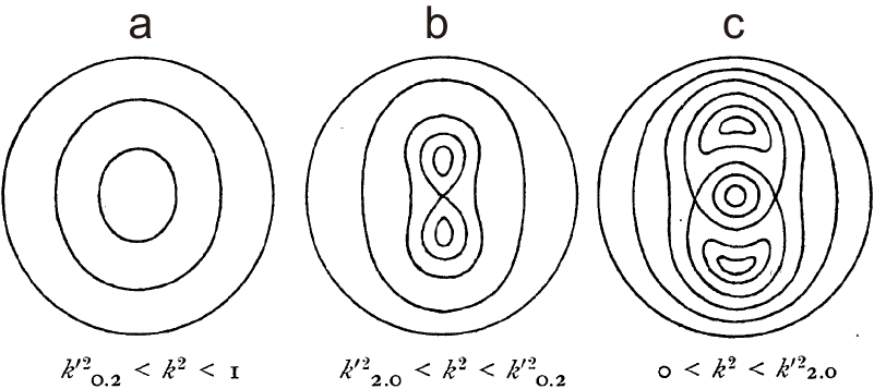
Figure 17: Transcription of von Zeipel’s Figs. Z8, Z9, Z10 on his pp. Z401–Z402 (Credit: John Wiley and Sons. Reproduced with permission). They represent schematic trajectories of equi-$R$ contours of the doubly averaged outer CR3BP on the $(e\cos g,e\sin g)$ plane. a: von Zeipel’s Fig. Z8 for the case when ${k^{\prime}}^{2}_{0.2}<k^{2}<1$. b: His Fig. Z9 for the case when ${k^{\prime}}^{2}_{2.0}<k^{2}<{k^{\prime}}^{2}_{0.2}$. c: His Fig. Z10 for the case when $0<k^{2}<{k^{\prime}}^{2}_{2.0}$.

Type of the local extremums

Similar to the discussion on the inner case (p. 5.6.2), von Zeipel next investigates the characteristics of the points $(x,y)=(\pm e^{\prime}_{2.0},0)$ and $(0,\pm e^{\prime}_{0.2})$ as local extremums of $R$ (pp. Z400–Z401). For this purpose he focuses on inspecting the sign of the three second derivatives $\frac{\partial^{2}R}{\partial g{}^{2}}$, $\frac{\partial^{2}R}{\partial e\partial g}$, $\frac{\partial^{2}R}{\partial e{}^{2}}$ when $\cos 2g=\pm 1$.

As for $\frac{\partial^{2}R}{\partial g{}^{2}}$, from Eq. (Z98-323) we get straightaway its general form as

$$\frac{\partial^{2}R}{\partial g{}^{2}}=-{\alpha^{\prime}}^{5}\frac{135}{64}\frac{e^{2}\sin^{2}I\left(1-\frac{7}{6}\sin^{2}I\right)}{\left(1-e^{2}\right)^{\frac{7}{2}}}\cos 2g.$$ (349)

From Eqs. (Z103-340) and (Z104-341), we know that $k^{2}\sim\frac{1-e^{2}}{5}$ both at $e^{2}={e^{\prime}}^{2}_{2.0}$ and ${e^{\prime}}^{2}_{0.2}$ if $\alpha^{\prime}\ll 1$. This means

$$\sin^{2}I =1-\cos^{2}I$$ (350)

$$=1-\frac{k^{2}}{1-e^{2}}\sim\frac{4}{5},$$

and therefore

$$1-\frac{7}{6}\sin^{2}I\sim\frac{1}{15}>0.$$ (351)

From Eqs. (349) and (351), we can conclude that

• When $\cos 2g=+1$, $\frac{\partial^{2}R}{\partial g{}^{2}}<0$ at $(x,y)=(\pm e^{\prime}_{2.0},0)$.

• When $\cos 2g=-1$, $\frac{\partial^{2}R}{\partial g{}^{2}}>0$ at $(x,y)=(0,\pm e^{\prime}_{0.2})$.

$\frac{\partial^{2}R}{\partial e\partial g}$ has the simplest form. From Eq. (Z98-323) we get

$$\frac{\partial^{2}R}{\partial e\partial g}=0,$$ (352)

when $\cos 2g=\pm 1$. This is because all the terms of $\frac{\partial^{2}R}{\partial e\partial g}$ contain $\sin 2g$ as a factor which is zero when $\cos 2g=\pm 1$.

$\frac{\partial^{2}R}{\partial e{}^{2}}$ is more complicated. In addition, similar to the case of the inner problem (p. 5.6.2), von Zeipel’s original description seems very terse. Let us add a complementary description as to how we should deal with $\frac{\partial^{2}R}{\partial e{}^{2}}$.

We again adopt the identity (276) for $\frac{\partial^{2}R}{\partial e{}^{2}}$ of the outer problem. The resulting $\frac{\partial^{2}R}{\partial e{}^{2}}$ in its general form turns out to be rather complicated, and we have considered it in Appendix B. Then we do the following:

• Substitute $e^{2}={e^{\prime}}^{2}_{2.0}$ of (Z101-331) into $\left.\frac{\partial^{2}R}{\partial e{}^{2}}\right|_{\cos 2g=+1}$

• Substitute $e^{2}={e^{\prime}}^{2}_{0.2}$ of (Z101-331) into $\left.\frac{\partial^{2}R}{\partial e{}^{2}}\right|_{\cos 2g=-1}$

As a result, we get

$$\frac{\partial^{2}R}{\partial e{}^{2}}=-\frac{3\sqrt{5}\left(5k^{2}-1\right)}{2500k^{\frac{7}{2}}}{\alpha^{\prime}}^{3}+O\bigl{(}{\alpha^{\prime}}^{5}\bigr{)},$$ (353)

at both the points $(x,y)=(\pm e^{\prime}_{2.0},0)$ and $(x,y)=(0,\pm e^{\prime}_{0.2})$. If we ignore the terms of $O\bigl{(}{\alpha^{\prime}}^{5}\bigr{)}$ in the right-hand side, it is clear that $\frac{\partial^{2}R}{\partial e{}^{2}}$ in Eq. (353) monotonically decreases with the increase of $k^{2}$. And yet, it remains positive while $k^{2}<\frac{1}{5}$. We should recall that $k^{2}<\frac{1}{5}$ is necessary for ${e^{\prime}}^{2}_{2.0}$ and ${e^{\prime}}^{2}_{0.2}$ to remain positive (see Eqs. (Z103-340) and (Z104-341)). Therefore we can conclude that

$$\frac{\partial^{2}R}{\partial e{}^{2}}>0,$$ (354)

at all the four points $(x,y)=(\pm e^{\prime}_{2.0},0)$ and $(0,\pm e^{\prime}_{0.2})$, if $\alpha^{\prime}\ll 1$. In Appendix B we show the actual expression of the terms at $O\bigl{(}{\alpha^{\prime}}^{5}\bigr{)}$ in the right-hand side of Eq. (353) which von Zeipel omitted. It turned out that the conclusion of Eq. (354) remains true even if we include the $O\bigl{(}{\alpha^{\prime}}^{5}\bigr{)}$ terms.

Collecting all the results presented in Section Z22, von Zeipel states the following proposition about the location of local extremums of $R$ in the outer case when $\alpha^{\prime}$ is small:

“If ${k^{\prime}}^{2}_{0.2}<k^{2}<1$, the function $R$ does not possess maxima or minimaxima in the domain $e<k^{\prime}$, and takes a single minimum at $e=0$.

— If ${k^{\prime}}^{2}_{2.0}<k^{2}<{k^{\prime}}^{2}_{0.2}$, the function $R$ has no maximum in the domain $e<k^{\prime}$ and possesses only one minimaximum in this area, situated at the origin $e=0$, and only two minima at the points $g=\pm\frac{\pi}{2}$, $e=e^{\prime}_{0.2}$.

— Finally, if $0<k^{2}<{k^{\prime}}^{2}_{2.0}$, the function $R$ possesses a single maximum in the domain $e<k^{\prime}$ situated at the origin $e=0$, only two minimum at the points $g=\pm\frac{\pi}{2}$, $e=e^{\prime}_{0.2}$ and only two minimaxima at the points $g=0$ or $\pi$, $e=e^{\prime}_{2.0}$.” (p. Z402)

After these considerations, von Zeipel shows schematic plots of equi-$R$ curves on the $(e\cos g,e\sin g)$ plane as his Figs. Z8, Z9, and Z10 for illustrating the circumstances. We transcribed them here as our Fig. 17. Through von Zeipel’s figures, it is obvious that the topology of the equi-$R$ contours qualitatively changes across $k^{2}={k^{\prime}}^{2}_{2.0}$ and $k^{2}={k^{\prime}}^{2}_{0.2}$. Since the difference between ${k^{\prime}}^{2}_{2.0}$ and ${k^{\prime}}^{2}_{0.2}$ is generally slight (see Eq. (Z101-331)), the parameter space that realizes the second case $\bigl{(}{k^{\prime}}^{2}_{2.0}<k^{2}<{k^{\prime}}^{2}_{0.2}\bigr{)}$ is narrow (Fig. 17b). We will present our own numerical demonstrations in Section 5.7.4 to reproduce his schematic plots.

5.7.3 When $\alpha^{\prime}$ is not so small

In Section Z23, von Zeipel deals with the doubly averaged outer CR3BP when $\alpha^{\prime}$ (or $a^{\prime}$ in his notation) is not negligibly small. In this regard, Section Z23 comprises the counterpart of Z17 that is on the inner problem. von Zeipel takes care of this task again through a numerical method. The particular focus of this section lies in showing that the doubly averaged disturbing function $R$ presented as Eq. (Z99-326) takes a local minimum at the origin $(x,y)=(0,0)$ under some condition, even when $\alpha^{\prime}$ is arbitrary. His method to derive numerical values of $R$ seems to follow what was presented in Section Z17. Probably due to this reason, his presentation of the mathematical procedures used in Section Z23 is brief and concise. Let us show its summary in what follows.

Similar to Eqs. (294), (280), and (281) presented in his Section Z17, von Zeipel first introduces new coefficients ${b^{\prime}}^{i.j}$, ${c^{\prime}}^{i.j}$, ${e^{\prime}}^{i.j}$ through the following definitions:

$$\left[1+{\alpha^{\prime}}^{2}-2\alpha^{\prime}\left(\mu\cos M+\nu\cos N\right)\right]^{-\frac{1}{2}}$$

$$\quad={b^{\prime}}^{0.0}+2{b^{\prime}}^{1.0}\cos M+2{b^{\prime}}^{0.1}\cos N$$

$$\quad\quad+4{b^{\prime}}^{1.1}\cos M\cos N+\cdots,$$ (355)

$$\left[1+{\alpha^{\prime}}^{2}-2\alpha^{\prime}\left(\mu\cos M+\nu\cos N\right)\right]^{-\frac{3}{2}}$$

$$\quad={c^{\prime}}^{0.0}+2{c^{\prime}}^{1.0}\cos M+2{c^{\prime}}^{0.1}\cos N$$

$$\quad\quad+4{c^{\prime}}^{1.1}\cos M\cos N+\cdots,$$ (356)

$$\left[1+{\alpha^{\prime}}^{2}-2\alpha^{\prime}\left(\mu\cos M+\nu\cos N\right)\right]^{-\frac{5}{2}}$$

$$\quad={e^{\prime}}^{0.0}+2{e^{\prime}}^{1.0}\cos M+2{e^{\prime}}^{0.1}\cos N$$

$$\quad\quad+4{e^{\prime}}^{1.1}\cos M\cos N+\cdots.$$ (357)

The coefficients ${b^{\prime}}^{i.j}$, ${c^{\prime}}^{i.j}$, ${e^{\prime}}^{i.j}$ defined for the outer problem in Eqs. (355), (356) and (357), and $b^{i.j}$, $c^{i.j}$, $e^{i.j}$ defined for the inner problem in Eqs. (294), (280) and (281), are connected through the following relationship:

$$\alpha^{\frac{1}{2}}b^{i.j} ={\alpha^{\prime}}^{\frac{1}{2}}{b^{\prime}}^{i.j},$$ (Z105-357)

$$\alpha^{\frac{3}{2}}c^{i.j} ={\alpha^{\prime}}^{\frac{3}{2}}{c^{\prime}}^{i.j},$$

$$\alpha^{\frac{5}{2}}e^{i.j} ={\alpha^{\prime}}^{\frac{5}{2}}{e^{\prime}}^{i.j}.$$

Then, von Zeipel expresses $R^{\prime}_{2.0}$ and $R^{\prime}_{0.2}$ in Eq. (Z99-326) using ${b^{\prime}}^{i.j}$, ${c^{\prime}}^{i.j}$, ${e^{\prime}}^{i.j}$ and $\alpha^{\prime}$ as follows:

$$R^{\prime}_{2.0} =-\alpha^{\prime}{c^{\prime}}^{1.1}+\frac{1}{2}{\alpha^{\prime}}^{2}\left({c^{\prime}}^{1.0}+{c^{\prime}}^{0.1}\right),$$ (Z106-358)

$$R^{\prime}_{0.2} =\alpha^{\prime}{c^{\prime}}^{1.1}-\frac{1}{4}{\alpha^{\prime}}^{2}\left({c^{\prime}}^{1.0}+{c^{\prime}}^{0.1}\right)$$

$$\quad+\frac{3}{4}{\alpha^{\prime}}^{2}k\left({c^{\prime}}^{1.0}-{c^{\prime}}^{0.1}\right)$$

$$\quad\quad-\frac{3}{4}{\alpha^{\prime}}^{3}\left(1-k^{2}\right)\left({e^{\prime}}^{0.0}-{e^{\prime}}^{1.1}\right).$$

Using the formulas (Z105-357), (Z106-358) and others, von Zeipel calculates the actual numerical values of $R^{\prime}_{2.0}$ and $R^{\prime}_{0.2}$. He tabulated them on an unnumbered table (pp. Z403–Z404). The table shows the values of $R^{\prime}_{2.0}$ and $R^{\prime}_{0.2}$, using $I_{0}(=\cos^{-1}k)$ and $\alpha^{\prime}$ as parameters. Similar to the unnumbered table for the inner case (pp. Z389–Z390), the range of $I_{0}$ is from 0 to $90^{\circ}$ with an interval of $10^{\circ}$, and the range of $\alpha^{\prime}$ is from 0.4 and 0.9 with an interval of 0.1. Instead of transcribing the table in this monograph, we make visual plots of their values in our Fig. 18.

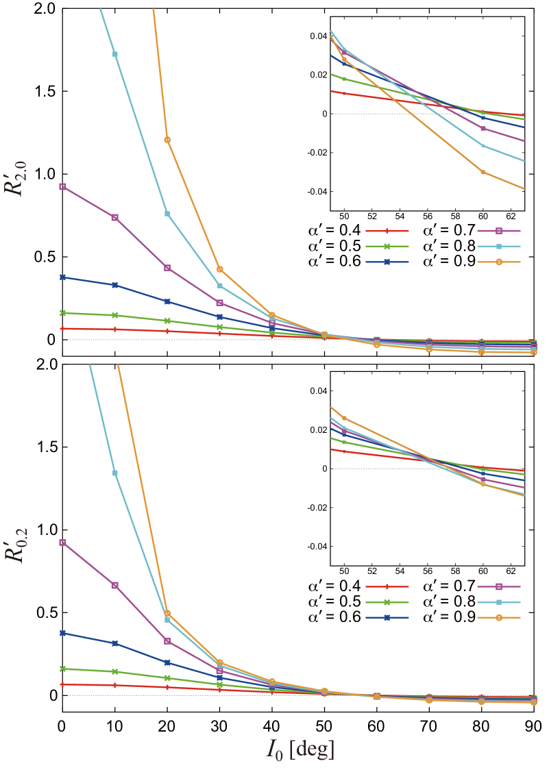
Figure 18: Dependence of the values of $R^{\prime}_{2.0}$ (upper panel) and $R^{\prime}_{0.2}$ (lower panel) on $I_{0}=\cos^{-1}k$ and on $\alpha^{\prime}$. For magnifying the near-zero part of $R^{\prime}_{2.0}$ and $R^{\prime}_{0.2}$, we placed inlets at the top right of both the panels. All the plots are based on the tabulated numerical values on an unnumbered table in von Zeipel (1910, pp. Z403–Z404).

The largest difference between the outer case and the inner case is that both the components ($R^{\prime}_{2.0}$ and $R^{\prime}_{0.2}$) can be zero in the outer case (Fig. 18). Meanwhile in the inner case, one of the components $(R_{2.0})$ always stays positive, and it is likely that $R_{2.0}$ never subceeds zero (Fig. 14). Let us cite von Zeipel’s description of his own result:

“We see from the table that the equation $R^{\prime}_{2.0}=0$ always has a root $I_{0}=I^{\prime}_{2.0}=\arccos k^{\prime}_{2.0}$ if $\alpha^{\prime}\leq 0.9$, and the equation $R^{\prime}_{0.2}=0$ also has a root $I_{0}=I^{\prime}_{0.2}=\arccos k^{\prime}_{0.2}$ if $\alpha^{\prime}\leq 0.9$.” (p. Z403)

This statement is followed by his observation:

“It also appears that

$$\begin{array}[]{ccc}R^{\prime}_{2.0}>0&{\rm if}&{k^{\prime}}^{2}_{2.0}<k^{2}<1\\ R^{\prime}_{2.0}<0&{\rm if}&0<k^{2}<{k^{\prime}}^{2}_{2.0}\\ R^{\prime}_{0.2}>0&{\rm if}&{k^{\prime}}^{2}_{0.2}<k^{2}<1\\ R^{\prime}_{0.2}<0&{\rm if}&0<k^{2}<{k^{\prime}}^{2}_{0.2}\mbox{.''}\\ \end{array}$$

(p. Z403)

By interpolating the numerical values of $R^{\prime}_{2.0}$ and $R^{\prime}_{0.2}$, von Zeipel calculated the numerical values of $I^{\prime}_{2.0}$ and $I^{\prime}_{0.2}$ which satisfy the equations (330) and (331) at each $\alpha^{\prime}$. He tabulated the result in an unnumbered table at the bottom of p. Z403. We transcribed the unnumbered table as our Table 3 (we will also visualize his results later).

Table 3: Transcription of an unnumbered table in von Zeipel (1910, p. Z403). The unit of $I^{\prime}_{2.0}$ and $I^{\prime}_{0.2}$ is the degree. See also Fig. 22 for a visualization of the tabulated values.

$\alpha^{\prime}$	$0.0$	$0.4$	$0.5$	$0.6$	$0.7$	$0.8$	$0.9$
$I^{\prime}_{2.0}$	$63.43$	$61.43$	$60.34$	$59.06$	$57.56$	$55.95$	$54.1$
$I^{\prime}_{0.2}$	$63.43$	$60.89$	$59.67$	$58.38$	$57.25$	$56.6$	$57.2$

From the results tabulated in our Table 3, von Zeipel makes an observation as follows:

“We see that the quantity $I^{\prime}_{2.0}-I^{\prime}_{0.2}$ is positive when $0<\alpha^{\prime}<0.74\cdots$ and negative if $\alpha^{\prime}>0.74\cdots$.” (p. Z404)

Then, through the above observation, he subsequently states the following theorem:

“The functions ${k^{\prime}}^{2}_{2.0}$ and ${k^{\prime}}^{2}_{0.2}$ being thus defined, we can state, as demonstrated, the following theorem:

At the origin $x=y=0$, the function $R$ becomes minimum if ${k^{\prime}}^{2}>{k^{\prime}}^{2}_{2.0}$ and if ${k^{\prime}}^{2}>{k^{\prime}}^{2}_{0.2}$; [$R$] becomes a saddle point if ${k^{\prime}}^{2}$ is between ${k^{\prime}}^{2}_{2.0}$ and ${k^{\prime}}^{2}_{0.2}$; [and $R$] becomes maximum if $k^{2}<{k^{\prime}}^{2}_{2.0}$ and $k^{2}<{k^{\prime}}^{2}_{0.2}$.” (p. Z404)

As a natural consequence of the above theorem, von Zeipel immediately states another theorem as follows:

“The necessary and sufficient condition for the eccentricity of the orbit of an infinitely small mass located outside the disturbing planet to be always small, if it is small at a given moment, is that the inclination of the orbit is not located between the two angles $I^{\prime}_{2.0}$ and $I^{\prime}_{0.2}$. (In this statement we have neglected the disturbing mass and the square of the eccentricity.)” (p. Z404)

As for the last sentence in parentheses “In this statement we have neglected the disturbing mass and the square of the eccentricity,” we interpret this that von Zeipel assumes that the mass of the perturbing body (Jupiter) is much smaller than the mass of the central object (Sun) in his setting. Also, we are aware that the terms higher than the square of the eccentricity $\left(e^{2}\right)$ have been neglected in this section, because von Zeipel just uses the lowest-order components ($R^{\prime}_{2.0}x^{2}$ and $R^{\prime}_{0.2}y^{2}$) in the two-variable Taylor expansion (Z99-326).

von Zeipel concludes Section Z23 by making the following statement. This statement seems to be a summary of what he discovered through the discussion in this section:

“Asteroids exterior at the disturbing planet thus belong to two categories. In the first category, the inclinations are smaller than ${I^{\prime}}^{2}_{2.0}$ and ${I^{\prime}}^{2}_{0.2}$; in the second, they are larger than these quantities.

We have demonstrated at no. Z22 that the function $R$ possesses minimum values at two symmetric points

$$x=0,\quad y=\pm e^{\prime}_{0.2}$$

if $\alpha^{\prime}$ is small and if $k^{2}<{k^{\prime}}^{2}_{0.2}$. It seems very likely that these minima exist for appropriate values of ${k^{\prime}}^{2}$, as long as $\alpha^{\prime}<0.74\cdots$ (value of $\alpha^{\prime}$ which makes $k^{\prime}_{0.2}=k^{\prime}_{2.0}$). If instead $\alpha^{\prime}>0.74\cdots$, it is probable that the two symmetric minima are on the axis of $x$, at least for the appropriate values of ${k^{\prime}}^{2}<{k^{\prime}}^{2}_{2.0}$. But for rigorously demonstrating the existence of these minima and for determining the position, it would be necessary to resort to numerical calculations.” (pp. Z404–Z405)

It is not surprising for us to know that von Zeipel did not actually carry out the “numerical calculations” for demonstrating the existence of the local minima of $R$ along the $x$-axis when $\alpha^{\prime}$ is large. Such a numerical analysis must have been formidable in his time. Since studies on the doubly averaged outer CR3BP are less often encountered than the inner one even in modern days, we have not found relevant literature that confirms von Zeipel’s theorem (or conjecture) stated above. Therefore in the next part of this monograph (Section 5.7.4), we carry out a numerical confirmation of the theorem and conjecture that von Zeipel stated for the outer case when $\alpha^{\prime}$ is not negligibly small.

5.7.4 Numerical confirmation

Here we carry out several numerical experiments in order to confirm how accurate (or inaccurate) von Zeipel’s theory is on the doubly averaged outer CR3BP that has been presented in this monograph. Naturally, the contents in what follows are not included in von Zeipel’s original work.

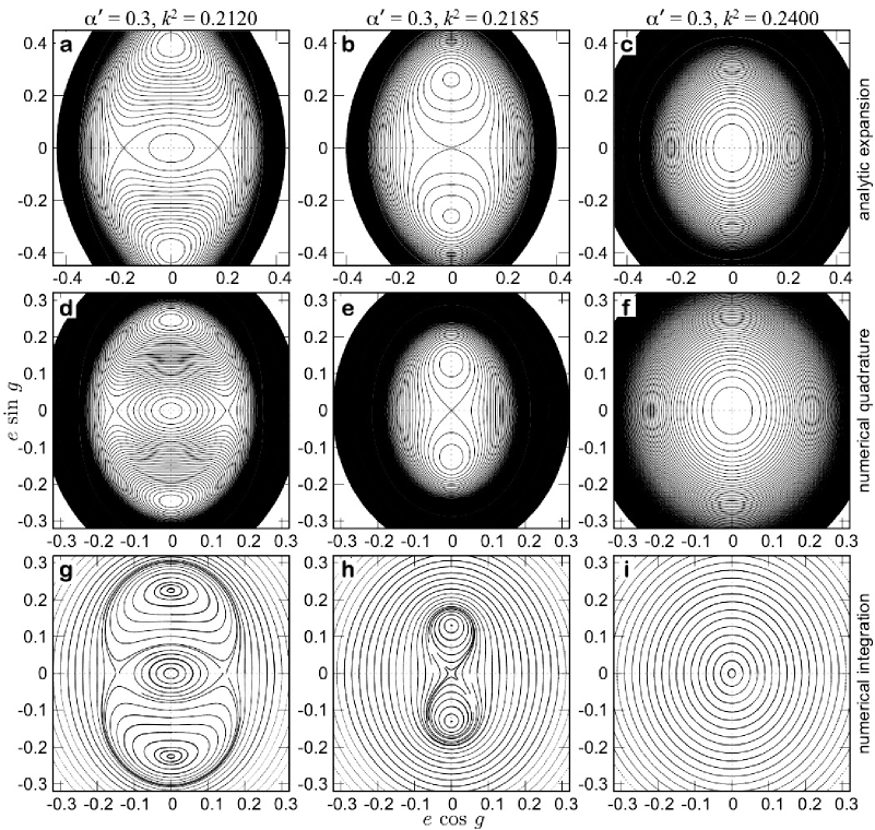
Figure 19: Equi-potential contours of the outer CR3BP plotted on the $(x,y)=(e\cos g,e\sin g)$ plane. The top row (a, b, c): Results obtained from von Zeipel’s analytic expansion of $R$ presented as Eqs. (Z97-322) and (Z98-323). The middle row (d, e, f): Results obtained from the numerical quadrature defined by Eq. (K09-53). The bottom row (g, h, i): Results obtained from the direct numerical integration of the equations of motion. The columns are categorized by the parameter sets $(\alpha^{\prime},k^{2})$ that are used: $(\alpha^{\prime},k^{2})=(0.3,0.2120$) for the panels in the left column (a, d, g), $(0.3,0.2185$) for the panels in the middle column (b, e, h), and $(0.3,0.2400$) for the panels in the right column (c, f, i). Note that the $x$- and $y$-ranges are both from $-0.45$ to $+0.45$ only in the top row (a, b, c), while they are from $-0.32$ to $+0.32$ in the middle and bottom rows (d, e, f, g, h, i).

Equi-potential contours (when $\alpha^{\prime}\ll 1$)

First, let us reproduce the equi-potential contours given in von Zeipel’s schematic Figs. Z8, Z9, and Z10 (transcribed as our Fig. 17). We use the doubly averaged disturbing function $R$ in Eq. (Z97-322) that von Zeipel derived. As we learned, the leading-order term of $R$ ($R^{\prime}_{3}$ in Eq. (Z98-323)) does not depend on the variable $g$. $R$’s dependence on $g$ shows up in $R^{\prime}_{5}$ and the higher-order terms. Therefore, to see the dependence of $R$ on $g$, we need to choose $\alpha^{\prime}$ which is small but not too small. If we adopt too small a value of $\alpha^{\prime}$, the higher-order terms would become extremely tiny, and the dependence of $R$ on $g$ would vanish. For this reason we chose $\alpha^{\prime}=0.3$ as an example here. This yields ${k^{\prime}}^{2}_{2.0}\sim 0.2162$ and ${k^{\prime}}^{2}_{0.2}\sim 0.2216$ from Eq. (Z101-331).

We reproduced the equi-potential contours of $R$ using Eqs. (Z97-322) and (Z98-323), and presented the result as the top three panels (a, b, c) of Fig. 19 labeled as “analytic expansion” at the right edge. The three typical patterns of equi-potential curves that we saw in von Zeipel’s original drawing (Fig. 17) are well reproduced. When $k^{2}<{k^{\prime}}^{2}_{2.0}$ (Fig. 19a), we see a local maximum of $R$ at the origin $(x,y)=(0,0)$ together with a pair of local minima along the $y$-axis, as well as a pair of saddle points along the $x$-axis. When ${k^{\prime}}^{2}_{2.0}<k^{2}<{k^{\prime}}^{2}_{0.2}$ (Fig. 19b), we find the origin being a saddle point of $R$, and a pair of local minima along the $y$-axis shows up. When ${k^{\prime}}^{2}_{0.2}<k^{2}$ (Fig. 19c), the origin becomes a local minimum of $R$ which is its only local extremum. These results are consistent with von Zeipel’s statement given with his Figs. Z8–Z10 (our Fig. 17).

We would like readers to note that each of the panels a, b, c in Fig. 19 has an individual and different contour interval. They represent a fixed energy interval of the doubly averaged disturbing potential in each of the systems. Hence, regions with dense contours imply that the potential gradient is steep there. Then, the results in these panels indicate that the potential gradient around the origin $(0,0)$ is much less steep than in other regions where the contour density is much higher. Note also that we did not draw all the contours in the outermost part of the plots (near the panel edge) mainly because the contour intervals would become too narrow and it would make the plots too busy.

Second, we draw equi-$R$ curves using the same parameter set $\left(\alpha^{\prime},k^{2}\right)$ but through the numerical quadrature defined by Eq. (K09-53). The result is presented as the middle three panels (d, e, f) of Fig. 19 labeled as “numerical quadrature” at the right edge. We clearly see that each of them has similar topological patterns as those in the top three panels (a, b, c). There seems to be a slight difference in the locations of local extremums on the $x$- and $y$-axis: The local extremums in panels d, e, f in Fig. 19 are located closer to the origin compared with the panels a, b, c. Readers should note that we adopted the smaller plot ranges (from $-0.32$ to $+0.32$ for both $x$ and $y$) in the middle three panels d, e, f than those in the top three panels a, b, c (from $-0.45$ to $+0.45$). This is to show the detailed structure of the equi-$R$ curves near the origin in the middle three panels. The slight difference between the result of the numerical quadrature and that of the analytic expansion is probably caused by the fact that the expression of the analytic expansions in Eqs. (Z97-322) and (Z98-323) does not include higher-order terms such as $R^{\prime}_{7},R^{\prime}_{9},\cdots$ . We have confirmed that the locations of the local extremums obtained from the analytic expansion become more similar to those obtained from the numerical quadrature when we use expansions of even higher-orders (Ito, 2016).

We also carried out a set of direct numerical integration of the equations of motion for the outer CR3BP using the same three parameter sets of $\left(\alpha^{\prime},k^{2}\right)$. The numerical integration scheme is the same as what we used when drawing Fig. 8. We placed a perturber on a circular orbit with the semimajor axis $a^{\prime}=5.2042$ au. The integration result is presented as the bottom three panels (g, h, i) of Fig. 19 labeled as “numerical integration” at the right edge. The nominal stepsize of the integration is 20 days, and the total integration time is 1200 million years with a data output interval of 5000 years. Note that here we set the ratio of the perturber’s mass and the central mass as $9.5479194\times 10^{-5}$ which is close to $\frac{1}{10}$ of the mass ratio between Jupiter and the Sun. This is to avoid the inclusion of short periodic oscillations in the plots, and to clearly show the detailed structure of the equi-$R$ contours. The influence of the mass ratio is limited to the timescale of the orbital evolution of the perturbed body, and it does not affect the orbit’s secular topology (see the discussion in Section 2.3 on p. 2.3 of this monograph).

In the panels g, h, i of Fig. 19 that show the result of the direct numerical integration, the contour interval does not represent fixed intervals of disturbing potential. We placed the perturbed bodies initially along the $x$-axis on the $(e\cos g,e\sin g)$ plane. More specifically, we placed the perturbed bodies along the $x$-axis with an interval of initial eccentricity ($e_{0}$) as $\Delta e_{0}=0.02$. The minimum of $e_{0}$ in the panel g is $e_{0,\mathrm{min}}=0.02$, and the minimum of $e_{0}$ in the panels h and i is $e_{0,\mathrm{min}}=0.01$. We also placed several more perturbed bodies along the $y$-axis around the local minima with the same interval $\Delta e_{0}$. As for the initial argument of pericenter $g$, we basically selected $g=0$ and $\frac{\pi}{2}$, as well as $g=\pi$ and $\frac{3\pi}{2}$ when necessary. As we see, the trajectories obtained from the numerical integration (g, h, i), those obtained from the numerical quadrature (d, e, f), and those obtained from the analytic expansion of the doubly averaged disturbing function (a, b, c) agree well with each other. Note that some of the trajectories on the bottom two panels (g and h) are not completely closed. These trajectories are very close to the separatrix where it principally takes an infinite amount of time for the perturbed body to reach the saddle points. It seems that the integration period that we chose for the numerical orbit propagation to draw the panels g and h was not long enough for the trajectories to be closed.

Values of ${k^{\prime}}^{2}_{2.0},{k^{\prime}}^{2}_{0.2},I^{\prime}_{2.0},I^{\prime}_{0.2}$ (when $\alpha^{\prime}$ is not small)

Now, we move on to the case when $\alpha^{\prime}$ is not so small. First, let us calculate the critical inclinations $I^{\prime}_{2.0}=\cos^{-1}k^{\prime}_{2.0}$ and $I^{\prime}_{0.2}=\cos^{-1}k^{\prime}_{0.2}$, as well as their dependence on $\alpha^{\prime}$. They were discussed on p. 5.7.3 of this monograph, and von Zeipel’s calculation results are transcribed in our Table 3. He wrote that the sign of $I^{\prime}_{2.0}-I^{\prime}_{0.2}$ changes from positive to negative at $\alpha^{\prime}\sim 0.74$ (see p. 5.7.3 of this monograph). As for the inner CR3BP, we compared von Zeipel’s $I_{0.2}$ with Kozai’s limiting inclination $i_{0}$ (see our Fig. 15 and the accompanying discussion on p. 15). As for the outer CR3BP, we calculate the critical inclination values that are equivalent to $I^{\prime}_{2.0}$ and $I^{\prime}_{0.2}$ through numerical quadrature as follows.

For calculating $I^{\prime}_{2.0}$ and $I^{\prime}_{0.2}$, we need to obtain the values of $R$ along the $x$- and $y$-axis on the $(e\cos g,e\sin g)$ plane. Considering the symmetry of $R$, we carry out a series of numerical quadrature defined in Eq. (K09-53) only on the positive $x$-axis $(g=0)$ and the positive $y$-axis $(g=\frac{\pi}{2})$ using several parameter sets $\left(\alpha^{\prime},k^{2}\right)$. Then we observe the behavior of $R$, and estimate the sign of $\frac{\partial R}{\partial x}$ and $\frac{\partial R}{\partial y}$ around the origin $(0,0)$. As we saw in Section 5.7.3, there can be four patterns in the appearance of local extremums.

• Pattern 1.
  The origin $(0,0)$ makes a local maximum, and there shows up a pair of local minima on the $y$-axis, as well as a pair of saddle points on the $x$-axis. This pattern is seen in the left column panels (a, d, g) of Fig. 19. In this pattern, $R$ decreases both along the $x$- and $y$-directions from the origin $(0,0)$. Therefore we have

  $$\left.\frac{\partial R}{\partial x}\right|_{x=y=0}<0,\quad\left.\frac{\partial R}{\partial y}\right|_{x=y=0}<0.$$ (360)

• Pattern 2.
  The origin $(0,0)$ makes a saddle point, and there shows up a pair of local minima only on the $y$-axis. This pattern is seen in the middle column panels (b, e, h) of Fig. 19. In this pattern, $R$ decreases along the $y$-axis, and it increases along the $x$-axis from the origin. So we have

  $$\left.\frac{\partial R}{\partial x}\right|_{x=y=0}>0,\quad\left.\frac{\partial R}{\partial y}\right|_{x=y=0}<0.$$ (361)

• Pattern 3.
  The origin $(0,0)$ makes a local minimum, and no other local extremum exists. This pattern is seen in the right column panels (c, f, i) of Fig. 19. In this pattern, $R$ monotonically increases from the origin along any directions. Therefore we have

  $$\left.\frac{\partial R}{\partial x}\right|_{x=y=0}>0,\quad\left.\frac{\partial R}{\partial y}\right|_{x=y=0}>0.$$ (362)

• Pattern 4.
  There shows up a pair of local minima on the $x$-axis, and the origin $(0,0)$ makes a saddle point. This pattern is what von Zeipel predicted in his Section Z23 (see p. 5.7.3), but no figure has been given yet. In this pattern, $R$ would decrease from the origin along the $x$-axis, and it would increase along the $y$-axis. Therefore we would have

  $$\left.\frac{\partial R}{\partial x}\right|_{x=y=0}<0,\quad\left.\frac{\partial R}{\partial y}\right|_{x=y=0}>0.$$ (363)

Note that as long as the approximation is up to $O\left(e^{2}\right)$ as von Zeipel assumed (see p. 286), the $R$ values along the $x$- and the $y$-axis are equivalent to $R^{\prime}_{2.0}$ and $R^{\prime}_{0.2}$ themselves in Eqs. (Z99-326) and (Z100-327), respectively. In other words, we have in this approximation

$$\left.\frac{\partial R}{\partial x}\right|_{x=y=0} =\left.\frac{\partial R^{\prime}_{2.0}}{\partial x}\right|_{x=y=0},$$ (364)

$$\left.\frac{\partial R}{\partial y}\right|_{x=y=0} =\left.\frac{\partial R^{\prime}_{0.2}}{\partial y}\right|_{x=y=0}.$$ (365)

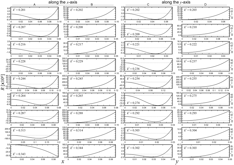
Figure 20: Values of the doubly averaged outer disturbing function $R$ obtained through the numerical quadrature (K09-53) along the positive $x$-axis $(g=0)$ and along the positive $y$-axis $(g=\frac{\pi}{2})$ with several $(\alpha^{\prime},k^{2})$ sets. The rows are, from the top, for $\alpha^{\prime}=0.1,0.2,0.3,\ldots,0.9$. The left two columns (A and B) are for $R$ along the $x$-axis, and the right two columns (C and D) are for $R$ along the $y$-axis. Note that the $R$ values are magnified by $10^{6}$ in all the panels: Their original magnitude is as small as $O(10^{-6})$ to $O(10^{-4})$ in our calculation. See Fig. 21 for comparison.

The purpose of our series of numerical quadrature is to investigate which set of $\left(\alpha^{\prime},k^{2}\right)$ realizes which of the above patterns 1, 2, 3, 4 (or the conditions (360), (361), (362), (363)). One of von Zeipel’s theoretical predictions that we learned in Section 5.7.3 tells us the following:

• The condition (360) is satisfied while $k^{2}$ is smaller than both ${k^{\prime}}^{2}_{2.0}$ and ${k^{\prime}}^{2}_{0.2}$. (Pattern 1)

• When ${k^{\prime}}^{2}_{2.0}<{k^{\prime}}^{2}_{0.2}$, if we fix $\alpha^{\prime}$ and gradually increase the value of $k^{2}$, we would reach a point where the status of the system changes from the condition (360) to the condition (361). The value of $k^{2}$ at this point would be equal to ${k^{\prime}}^{2}_{2.0}$, and the limiting inclination $I^{\prime}_{2.0}$ is calculated as $I^{\prime}_{2.0}=\cos^{-1}k^{\prime}_{2.0}$. (Pattern 2)

• If we further increase $k^{2}$ from this point, we would reach another point where the status of the system changes from the condition (361) to the condition (362). The value of $k^{2}$ at this point would be equal to ${k^{\prime}}^{2}_{0.2}$, and the limiting inclination $I^{\prime}_{0.2}$ is calculated as $I^{\prime}_{0.2}=\cos^{-1}k^{\prime}_{0.2}$. (Pattern 3)

• If ${k^{\prime}}^{2}_{2.0}>{k^{\prime}}^{2}_{0.2}$ is realized when $\alpha^{\prime}$ is large (as von Zeipel predicted), the condition (363) can take place in a certain range of $k^{2}$. (Pattern 4)

Bearing the above circumstances in mind, we calculated the values of $R$ along the $x$- and $y$-axis through the series of numerical quadrature. As for the value of $\alpha^{\prime}$, we varied it from $\alpha^{\prime}=0$ to $0.95$ in steps of $0.05$. As for the value of $k^{2}$, we started from $k^{2}=0.200$ and increased it in steps of $0.001$. We plotted the resulting values of $R$ along the $x$- and $y$-axis with several $\alpha^{\prime}$ and $k^{2}$ in Fig. 20.

In Fig. 20, the panels in the left two columns depict $R$ along the $x$-axis just before (the column A) and just after (the column B) $\left.\frac{\partial R}{\partial x}\right|_{x=y=0}$ changes its sign. The panels in the right two columns depict $R$ along the $y$-axis just before (the column C) and just after (the column D) $\left.\frac{\partial R}{\partial y}\right|_{x=y=0}$ changes its sign. For example, when $\alpha^{\prime}=0.7$ (see the seventh row from the top), $\left.\frac{\partial R}{\partial x}\right|_{x=y=0}$ seems negative while $k^{2}\leq 0.287$ (the panel in the column A) but it seems to turn positive while $k^{2}\geq 0.288$ (the panel in the column B). Thus, we conclude that the ${k^{\prime}}^{2}_{2.0}$ value lies somewhere between 0.287 and 0.288 when $\alpha^{\prime}=0.7$. Similarly, $\left.\frac{\partial R}{\partial y}\right|_{x=y=0}$ seems negative while $k^{2}\leq 0.292$ (the panel in the column C) but it seems to turn positive while $k^{2}\geq 0.293$ (the panel in the column D). Thus, we conclude that the ${k^{\prime}}^{2}_{0.2}$ value lies somewhere between 0.292 and 0.293 when at $\alpha^{\prime}=0.7$.

Looking at the panels in the columns A and C of Fig. 20, we can visually locate the local minima of $R$ with our eyes. However, we do not see any local extremums in the bottom panel of the column A when $(\alpha^{\prime},k^{2})=(0.9,0.343)$. $\left.\frac{\partial R}{\partial x}\right|_{x=y=0}$ seems to remain negative throughout this panel. From the analogy of other panels in this column, we may want to imagine the existence of a local minimum somewhere along the $x$-axis beyond the range of this plot. However, we cannot actually identify the location of a local minimum in this case. This is because, in the large $\alpha^{\prime}$ range such as $\alpha^{\prime}=0.9$, the line of orbit intersection takes place relatively close to the origin, $(0,0)$. To better illustrate the circumstance, we extended the $x$-range of this panel and redrew it as Fig. 21. In this figure, we see that the line of orbit intersection happens just before $x=0.1$, and $R$ shows a steep and rapid change beyond this point. Readers should pay attention to the huge magnitude difference of $R$ between inside and outside this border. See Section 5.8 of this monograph (p. 5.8) for more detail about the local extremums that occur beyond the line of orbit intersection.

Figure 21: An extended plot of the bottom panel in the left-most column (A) of Fig. 20. This shows the changing values of $R$ along the $x$-axis when $(\alpha^{\prime},k^{2})=(0.9,0.343$). The location of orbit intersection of the perturbing body and the perturbed body at $x\sim 0.09$ is indicated by an arrow. Note that, unlike in Fig. 20, the vertical scale is not magnified in this panel. This means that the magnitude of $R$ is $O(10^{-5})$ when $x\lesssim 0.09$, while it is $O(1)$ when $x\gtrsim 0.09$.

Using the numerical quadrature result that is partly presented in Fig. 20, we calculated ${k^{\prime}}^{2}_{2.0}$ and ${k^{\prime}}^{2}_{0.2}$, as well as $I^{\prime}_{2.0}(=\cos^{-1}k^{\prime}_{2.0})$ and $I^{\prime}_{0.2}(=\cos^{-1}k^{\prime}_{0.2})$, all as functions of $\alpha^{\prime}$. Our calculation result is summarized in Fig. 22 together with the values that von Zeipel presented for comparison. Fig. 22a shows the dependence of ${k^{\prime}}^{2}_{2.0}$ and ${k^{\prime}}^{2}_{0.2}$ on $\alpha^{\prime}$. We plotted von Zeipel’s ${k^{\prime}}^{2}_{2.0}$ and ${k^{\prime}}^{2}_{0.2}$ in the range of $0.4\leq\alpha^{\prime}\leq 0.9$. We obtained them by converting his $I^{\prime}_{2.0}$ and $I^{\prime}_{0.2}$ tabulated in Table 3 into ${k^{\prime}}^{2}_{2.0}$ and ${k^{\prime}}^{2}_{0.2}$. Fig. 22b shows the dependence of $I^{\prime}_{2.0}$ and $I^{\prime}_{0.2}$ on $\alpha^{\prime}$. von Zeipel’s $I^{\prime}_{2.0}$ and $I^{\prime}_{0.2}$ are extracted from Table 3 and plotted in this panel. These panels clearly indicate that the agreement between von Zeipel’s result and our numerical result is excellent, with just a slight difference when $\alpha^{\prime}=0.90$. This figure exemplifies the correctness of von Zeipel’s theory and his calculations on the doubly averaged outer CR3BP, even when $\alpha^{\prime}$ is not small. To our knowledge, this type of quantitative comparison has never been done with the doubly averaged outer CR3BP over this extensive range of $\alpha^{\prime}$.

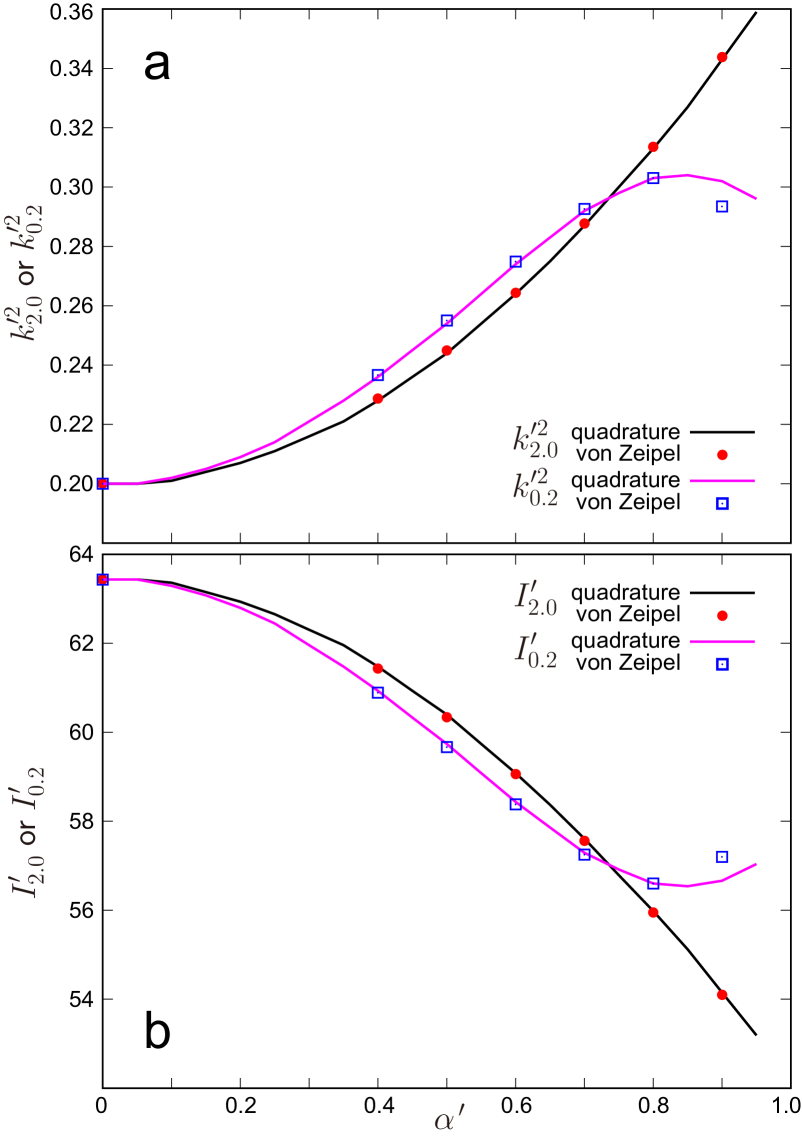
Figure 22: a: Actual values of ${k^{\prime}}^{2}_{2.0}$ (the black solid line) and ${k^{\prime}}^{2}_{0.2}$ (the magenta solid line) and their dependence on $\alpha^{\prime}$ estimated from our numerical quadrature. We also converted von Zeipel’s calculation result on $I^{\prime}_{2.0}$ and $I^{\prime}_{0.2}$ (see Table 3) into ${k^{\prime}}^{2}_{2.0}=\cos^{2}I^{\prime}_{2.0}$ (the filled red circle) and ${k^{\prime}}^{2}_{0.2}=\cos^{2}I^{\prime}_{0.2}$ (the open blue square with a central dot), and plotted them in this panel. b: The corresponding values of $I^{\prime}_{2.0}$ (the black solid line) and $I^{\prime}_{0.2}$ (the magenta solid line) converted from ${k^{\prime}}^{2}_{2.0}$ and ${k^{\prime}}^{2}_{0.2}$ plotted in the panel a. von Zeipel’s numerical estimate summarized in Table 3 is also plotted: $I^{\prime}_{2.0}$ (the filled red circle) and $I^{\prime}_{0.2}$ (the open blue square with a central dot).

Equi-potential contours (when $\alpha^{\prime}$ is not small)

From the results presented in Figs. 20, 21, and 22, we have confirmed that von Zeipel’s theory seems valid and accurate in the doubly averaged outer CR3BP, even when $\alpha^{\prime}$ is not small. Let us further move on and make another confirmation in this case. In what follows, our discussion goes along with a new figure (Fig. 23). This figure is a counterpart of Fig. 19 that we had made for the small $\alpha^{\prime}$ systems. The new figure contains ten panels, showing various trajectories of perturbed bodies in the outer CR3BP on the $(x,y)=(e\cos g,e\sin g)$ plane. We employed two methods to draw the panels: Numerical quadrature of two kinds, and direct numerical integration of the equations of motion.

We first set $\alpha^{\prime}=0.6$, and chose relatively small $k^{2}$ values ($k^{2}=0.2600$ and $k^{2}=0.2650$). The $2\times 2$ panels in the left two columns (a, b, e, f) of Fig. 23 show the equi-potential contours in this parameter set. The panels a and b are based on the result obtained from numerical quadrature, and the panels e and f are based on the result obtained from direct numerical integration of the equations of motion. The methods of numerical quadrature and numerical integration are the same as what we used in Fig. 19. We placed a perturber on a circular orbit with the semimajor axis $a^{\prime}=5.2042$ au. In the numerical integration result shown in the panels e and f, the nominal stepsize is 20 days, and the total integration time is 200 million years with a data output interval of 1000 years. The ratio of the perturber’s mass and the central mass is $4.7739597\times 10^{-5}$ which is close to $\frac{1}{20}$ of the mass ratio of Jupiter and the Sun.

The left $2\times 2$ panels (a, b, e, f) of Fig. 23 reproduce well the topological characteristics of the equi-$R$ curves that von Zeipel predicted. From the preceding calculation result presented in Fig. 20, when $\alpha^{\prime}=0.6$ we found ${k^{\prime}}^{2}_{2.0}$ lies somewhere in $\mathopen{]}0.264,0.265\mathclose{[}$, and ${k^{\prime}}^{2}_{0.2}$ lies somewhere in $\mathopen{]}0.274,0.275\mathclose{[}$. Therefore, the plots with $k^{2}=0.260$ (panels a and e) correspond to the topological pattern of $R$ when $k^{2}<{k^{\prime}}^{2}_{2.0}$ (Pattern 1 on p. 5.7.4). In this case the origin $(0,0)$ makes a local maximum, and we see a pair of local minima along the $y$-axis together with a pair of saddle points along the $x$-axis. The topological pattern looks the same as that observed in the $\alpha^{\prime}\ll 1$ case (Figs. 19a, 19d, 19g), although the locations of the local extremums along the $x$- and $y$-axis seem slightly different. On the other hand, the plots with $k^{2}=0.265$ (panels b and f) correspond to the topological pattern of $R$ when ${k^{\prime}}^{2}_{2.0}<k^{2}<{k^{\prime}}^{2}_{0.2}$ (Pattern 2 on p. 5.7.4). In this case, we see a saddle point at the origin $(0,0)$ as well as a pair of local minima along the $y$-axis. Again, the topological pattern seems the same as that observed in the $\alpha^{\prime}\ll 1$ case (Figs. 19b, 19e, 19h).

So far, the predictions that von Zeipel made about the dynamical behavior of the perturbed body in the doubly averaged outer CR3BP seem correct. However if we go on and further increase $\alpha^{\prime}$, the situation changes drastically: We find a limitation, not only of von Zeipel’s predictions, but of the double averaging approximation itself—the influence of mean motion resonance emerges.

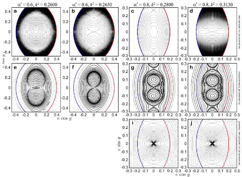
Figure 23: Equi-potential contours of the doubly averaged outer CR3BP on the $(x,y)=(e\cos g,e\sin g)$ plane when $\alpha^{\prime}$ is not small. The four panels in the top row (a, b, c, d) are the results obtained from the numerical quadrature defined by Eq. (K09-53). The four panels in the middle row (e, f, g, h) are the results obtained from the direct numerical integration of the equations of motion. The two panels in the bottom row (i, j) are the results obtained from the numerical quadrature that assumes the 5:7 mean motion resonance between the perturbed and perturbing bodies with a fixed critical argument of $5\lambda^{\prime}-7\lambda+2g=\pi$. The columns are categorized by the parameter set $(\alpha^{\prime},k^{2})$. We chose $(\alpha^{\prime},k^{2})=(0.6,0.2600$) for the leftmost column (the panels a, e), $(\alpha^{\prime},k^{2})=(0.6,0.2650$) for the second left column (the panels b, f), $(\alpha^{\prime},k^{2})=(0.8,0.2800$) for the second right column (the panels c, g, i), and $(\alpha^{\prime},k^{2})=(0.8,0.3130$) for the rightmost column (the panels d, h, j). Note that the $x$- and $y$-ranges are from $-0.48$ to $+0.48$ only in the $2\times 2$ panels in the left two columns (a, b, e, f), while they are from $-0.30$ to $+0.30$ in the $2\times 3$ panels in the right two columns (c, d, g, h, i, j). The partial red circles in each of the panels correspond to the negative sign in the first term of the left-hand side of Eq. (Z45-227), representing the location where the orbits of the perturbed and perturbing bodies intersect each other at the ascending node of the perturbed body. The partial blue circles correspond to the positive sign in the first term of the left-hand side of Eq. (Z45-227), representing the location where the orbits of the perturbed and perturbing bodies intersect each other at the descending node of the perturbed body.

As an example of our further investigation, we chose two more parameter sets of $(\alpha^{\prime},k^{2})=(0.8,0.2800)$ and $(\alpha^{\prime},k^{2})=(0.8,0.3130)$, and again carried out numerical quadrature. The calculation results are presented in the upper two panels in the right two columns of Fig. 23 (the panels c and d). From the preceding calculation result presented in Fig. 20, when $\alpha^{\prime}=0.8$ we found ${k^{\prime}}^{2}_{2.0}$ lies somewhere in $\mathopen{]}0.313,0.314\mathclose{[}$, and ${k^{\prime}}^{2}_{0.2}$ lies somewhere in $\mathopen{]}0.303,0.304\mathclose{[}$. Note that we have ${k^{\prime}}^{2}_{2.0}>{k^{\prime}}^{2}_{0.2}$ at this large value of $\alpha^{\prime}$ (see Fig. 22) which is a clear difference from the systems with small $\alpha^{\prime}$ that satisfy the opposite condition, Eq. (333). This collectively means that the value $k^{2}=0.280$ employed in the panel c is in the range of $k^{2}<{k^{\prime}}^{2}_{0.2}$, while the value $k^{2}=0.313$ employed in the panel d is (although marginally) in the range of ${k^{\prime}}^{2}_{0.2}<k^{2}<{k^{\prime}}^{2}_{2.0}$.

From the analogy of the result in the small $\alpha^{\prime}$ systems where ${k^{\prime}}^{2}_{2.0}<{k^{\prime}}^{2}_{0.2}$ is satisfied, we may want to anticipate that the topological pattern of the equi-$R$ curves in the systems with ${k^{\prime}}^{2}_{2.0}>{k^{\prime}}^{2}_{0.2}$ would be obtained by a $90^{\circ}$ rotation of the case of ${k^{\prime}}^{2}_{2.0}<{k^{\prime}}^{2}_{0.2}$. This anticipation is mostly correct, and the circumstance is realized in our numerical quadrature: Fig. 23c is close to a $90^{\circ}$ topological rotation of Fig. 23a, and Fig. 23d is close to a $90^{\circ}$ topological rotation of Fig. 23b. The truncation of equi-$R$ curves by the red and blue lines in the panels c and d (the lines representing orbit intersection) produces an apparent difference between them. For example, in the panel c we do not see any local minima along the $x$-axis that are supposed to correspond to the local minima observed in the panel a along its $y$-axis. Therefore, at this point we may want to believe that the following conjecture that von Zeipel stated at the end of his Section Z23 (p. 5.7.3 of this monograph) is true:

“If instead $\alpha^{\prime}>0.74\cdots$, it is probable that the two symmetric minima are on the axis of $x$, at least for the appropriate values of ${k^{\prime}}^{2}<{k^{\prime}}^{2}_{2.0}$.” (p. Z405)

However, the motion of the perturbed body in the actual (i.e. not averaged) CR3BP sometimes exhibits very different behavior from the averaged system. The panels g and h of Fig. 23 are typical examples of this sort. These panels are drawn through the results obtained from our direct numerical integration of the equations of motion. The parameters $(\alpha^{\prime},k^{2})$ used in the panels g and h are identical to those used in the panels c and d, respectively. Here is the detail of the numerical integration used to draw the panels g and h: the nominal stepsize is 4 days, and the total integration time is 30 million years with a data output interval of 500 years. The ratio of the perturber’s mass and the central mass is $9.5479194\times 10^{-6}$ which is close to $\frac{1}{100}$ of the mass ratio of Jupiter and the Sun. The reason for the small mass ratio is to avoid the occurrence of orbital instability of the perturbed body due to close encounters with the perturber near the orbit intersection lines. This is necessary because now $\alpha^{\prime}$ is as large as 0.8. We also chose a small value for the stepsize of numerical integration (4 days) for the same reason.

As is very clear in both the panels g and h, stationary points (local minima) show up along the $y$-axis. We do not see them in the panels c or d that are obtained from the result of numerical quadrature of the doubly averaged system. The overall trajectory shapes are very different between the panels c and g, and also between the panels d and h. In short, the doubly averaged approximation does not seem to work out in the system sampled here.

As far as we have investigated, the trajectory shape seen in Figs. 23g and 23h are related to the existence of the 5:7 mean motion resonance between the perturbing and perturbed bodies. The perturbed body’s secular motion in R3BP with mean motion resonance has been intensively studied since the mid-twentieth century (see an extensive review by Moons, 1996). Their relation to the Lidov–Kozai oscillation, as well as several practical methods to draw equi-$R$ contours for resonant systems, has been further developed (e.g. Kozai, 1985; Yoshikawa, 1989, 1990, 1991; Morbidelli, 2002; Gomes et al., 2005; Gallardo, 2006; Gomes, 2011). For visualizing the influence of the mean motion resonance in this case, we implemented a simple method devised by Kozai (1985) which is based on a more general theory on the secular motion of perturbed body in resonant dynamical systems (Giacaglia, 1968, 1969). The method of Kozai (1985) enables us to reduce the degrees of freedom of a resonant system to unity and draw its equi-$R$ trajectory. This method assumes that the critical argument $\sigma$ of mean motion resonance stays at a stable equilibrium, and always takes a single fixed value without an amplitude. In general, the critical argument $\sigma$ in CR3BP is defined as

$$\sigma=j_{1}\lambda^{\prime}+j_{2}\lambda+j_{3}g,$$ (366)

where $\lambda^{\prime}$ is the mean longitude of the perturbing body, and $\lambda$ is that of the perturbed body. We also have a relationship $j_{1}+j_{2}+j_{3}=0$, one of the so-called d’Alembert rules (e.g. Hamilton, 1994; Murray and Dermott, 1999). It is needless to say that $\sigma$ is not a constant in general resonant systems: Usually $\sigma$ exhibits libration with a certain amplitude and period. Kozai’s (1985) method does not consider the libration amplitude of $\sigma$ (i.e. it assumes the libration amplitude of $\sigma$ to be zero) for simplicity. This makes the calculation of doubly averaged disturbing function easier.

By inspecting the time variation of the perturbed body’s orbital elements in the systems presented in Figs. 23g and 23h, we confirmed that an argument $5\lambda^{\prime}-7\lambda+2g$ stays around $\pi$, although it oscillates with a certain amplitude. Therefore we presume that

$$\sigma=5\lambda^{\prime}-7\lambda+2g=\pi,$$ (367)

holds true in this case, and we carried out the numerical quadrature (K09-53) under the constraint of Eq. (367), following Kozai’s (1985) method. We show the resulting equi-potential trajectories in Figs. 23i and 23j. Although the approximation is crude, topological patterns of equi-potential curves seen in Figs. 23i and 23j seem similar to those in Figs. 23g and 23h: The origin $(0,0)$ is a saddle point, and another pair of saddle points shows up at $y\sim\pm 0.25$. Hence we believe this model explains the situation. A more sophisticated method for secular dynamics when mean motion resonance is at work, including the influence of $\sigma$’s time variation, will better reproduce the behavior of perturbed bodies exhibited in Fig. 23g and 23h. For recent, more advanced studies on the perturbed body’s secular motion in R3BP with mean motion resonances, consult Gallardo et al. (2012), Brasil et al. (2014), or Saillenfest et al. (2016, 2017a, 2017b).

Incidentally, note that the influence of mean motion resonance exists not only in the outer problem but also in the inner problem, although we do not give any examples. Kozai (1985) showed several examples along this line. However, we suspect the influence of mean motion resonance is more prominent in the outer problem than in the inner problem. This is because of the subtlety of the secular perturbation that causes the Lidov–Kozai oscillation in the outer problem compared with that in the inner problem. We had mentioned this point on p. 5.7.1 of this monograph.

As we have seen in this subsection, the conjectures that von Zeipel made for the doubly averaged outer CR3BP are largely justified through our numerical confirmation, except when major mean motion resonance is at work. The influence of mean motion resonance such as seen in Figs. 23i and 23j is relatively more apparent near the origin $(0,0)$ where the gradient of $R$ is small. On the other hand the influence seems weaker in regions further away from the origin, and the trajectories of the perturbed bodies largely follow what the doubly averaged disturbing function forecasts, particularly near and beyond the lines of orbit intersection (i.e. the red and blue curves in Figs. 23).

5.8 Cases of orbit intersection

We would say that, up to the previous subsection (Section 5.7) we have already written most of the things that we intended to write in this monograph. From here until the end of Section 5, we mention some of the additional features in von Zeipel’s work that are worth noting. Compared with what we have already reviewed, the later part (Sections Z24–Z29) of von Zeipel’s paper seems under development and largely remaining speculative, relying on rough approximations and assumptions. von Zeipel’s descriptions get lame and very terse, such as using a new function without giving its definition. Therefore, in what follows we do not present much detail of von Zeipel’s mathematical expositions; we just introduce his major conclusions.

von Zeipel’s Section Z24 (pp. Z405–Z413) is devoted to a series of mathematical demonstration in order to show that the doubly averaged disturbing function $R$ for CR3BP can have local minima in the third case that he mentioned in his Section Z16 (p. Z378, also p. 5.6 of this monograph)—when the two orbits intersect and they “behave like rings of a chain.” This includes a comprehensive study of $R$ in the domain $B$ or $B^{\prime}$ in Fig. 11, assuming that $k^{\prime}$ $\bigl{(}=\sqrt{1-k^{2}}\bigr{)}$ is small and also $\alpha^{\prime}-1$ (or its absolute value) is small.

von Zeipel’s major goals in Section Z24 seem to be as follows: First, expressing $R$ in the domain $B$ or $B^{\prime}$ of Fig. 11 using some holomorphic functions, and second, seeking all the solutions of the equations $\frac{\partial R}{\partial e}=\frac{\partial R}{\partial g}=0$ located in the domain $B$ or $B^{\prime}$. This section begins with an expression of $R$ in Eq. (Z93-301) using a single integral in the complex domain. von Zeipel gives the expression

$$R=\frac{\alpha^{\prime}}{2\pi\sqrt{-1}}\int_{|z=1|}\frac{r}{\sqrt{1+r^{2}}}F(\tau)\frac{dz}{z},$$ (Z110-367)

where $\sqrt{-1}$ denotes the imaginary unit, and $z$ is a complex variable defined as

$$\!\!\!\!\!\!\!z=\exp\sqrt{-1}u,$$ (Z109-368)

with eccentric anomaly $u$. The variable $\tau$ and the function $F(\tau)$ seen in Eq. (Z110-367) have already been defined and used in Eqs. (Z48-236) and (Z54-243). von Zeipel assumes a condition on $\alpha^{\prime}$ (or $a^{\prime}$ in his notation) as

$$\alpha^{\prime}=1+sk^{\prime}.$$ (Z107-369)

with a new parameter $s$ in the range of

$$-1<s<+1.$$ (371)

He also places a condition on eccentricity $e$ as

$$e=\varepsilon k^{\prime},$$ (Z108-371)

with a new parameter $\varepsilon$ in the range of

$$0\leq\varepsilon\leq 1.$$ (373)

Using the foregoing, von Zeipel shows that $R$ in Eq. (Z110-367) has the form

$$R=R_{1}\log{k^{\prime}}^{2}+R_{2}+R_{3}+R_{4}+R_{5},$$ (374)

or

$$R=R_{1}\log{k^{\prime}}^{2}+R^{\prime},$$ (Z130-374)

where $R_{2}$, $R_{3}$, $R_{4}$, $R_{5}$ and $R^{\prime}$ are holomorphic functions of orbital elements that are expressed by complex integrals. Their actual forms are shown as Eq. (Z126) on p. Z409 (which we do not reproduce here). After going through complicated calculations for obtaining actual but approximate function forms of $R_{1}$, $R_{2}$, $R_{3}$, $R_{4}$, $R_{5}$, von Zeipel eventually reaches the conclusion that $R$ in Eq. (Z130-374) has a minimum at $g=0$ when $k^{\prime}$ is small (i.e. when $\alpha^{\prime}\sim 1$ due to Eq. (Z107-369)). We cite what he says about it:

“The research of this issue were aimed at finding all the solutions of equations

$$\frac{\partial R}{\partial e}=\frac{\partial R}{\partial g}=0$$ (Z132-375)

that exist in the domain $B$, assuming that $k^{\prime}$ is small.

[$\cdots$]

Returning now to equations (Z132). For small values of $k^{\prime}$ they possess a single solution at the interior of domain $0\leq e\leq k^{\prime}$, $-\frac{\pi}{2}\leq g\leq+\frac{\pi}{2}$. This solution, which can be written

$$e=e_{1}=k^{\prime}\left(\frac{1}{\sqrt{2}}+{\cal B}\left(k^{\prime},k^{\prime}\log k^{\prime}\right)\right);\quad g=0$$ (Z134-376)

where ${\cal B}(0,0)=0$, corresponds to a minimum value of the function $R$, since $A(0)<0$, as we saw on page Z371.

Consider the equation

$$s=\frac{e_{1}}{k^{\prime}}.$$

For small values of $k^{\prime}$ it has a single root

$$s=s_{1}=\frac{1}{\sqrt{2}}+{\cal B}_{1}\left(k^{\prime},k^{\prime}\log k^{\prime}\right)$$

where ${\cal B}(0,0)=0$.” (pp. Z411–Z412)

Note that von Zeipel did not give any definitions of the functions ${\cal B}$ and ${\cal B}_{1}$ in the above except their boundary conditions (${\cal B}(0,0)=0$ and ${\cal B}_{1}(0,0)=0$). Note also that the quantity $A(0)$ in above once showed up in Section 5.5. See Eqs. (Z54-243), (Z55-244), (Z56-245) in p. 5.5.

von Zeipel continues and states a theorem as follows:

”We can now state the following theorem as shown:

For sufficiently small values of $k^{\prime}$, the function $R$ possesses neither maxima nor minimaxima in the domain $B$. If $|\alpha^{\prime}-1|>s_{1}k^{\prime}$, $R$ has no minima in this domain. If instead $|\alpha^{\prime}-1|<s_{1}k^{\prime}$, the function $R$ possesses in the domain $B$ only one minimum situated at the point (Z134).” (p. Z412)

Right after stating the above theorem, von Zeipel admits that he did not succeed in showing the existence of these minima when $\alpha^{\prime}-1$ or $k^{\prime}$ gets large:

“If the parameters $\alpha^{\prime}$ and $k^{\prime}$ vary, the points

$$e=e_{1},\quad g=0\>\>\mathrm{or}\>\>\pi,$$ (Z135-377)

where the function $R$ is minima in the domain $B$ or $B^{\prime}$, move. But it did not succeed in pursuing them analytically if $\alpha^{\prime}-1$ and $k^{\prime}$ cease to be small. My goal was only to direct the attention on the existence of these minima [that are] quite remarkable. Obviously it does not offer serious difficulty [in] finding their positions by calculating numerical values given for the parameters $\alpha^{\prime}$ and $k^{\prime}$.” (p. Z413)

As we have learned, the existence of local minima in $R$ means the existence of the Lindstedt series in their vicinity. In solar system dynamics, the corresponding periodic orbits would belong to a certain class of small bodies in a stable motion. von Zeipel specifically depicts the characteristics of the orbits in this state as follows:

“We can apply the result of this issue by calculating, according to no. Z7, Z8 and Z9, the series of Lindstedt, which exist when the elements are in the vicinity of the points (Z135). The corresponding orbits belong to a certain class of comets in stable motion. In these orbits, the semimajor axis, eccentricity and inclination are more or less almost constant; the perihelion distance to the node is still close to 0 or $\pi$; the line of nodes has a retrograde motion; Finally, the orbits of the comet and of the disturbing planet are situated relative to the other like the rings of a chain.” (p. Z413)

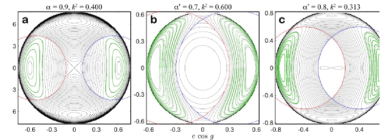
Figure 24: Equi-potential contours and trajectories of fictitious perturbed bodies that realize the circumstance of “rings of a chain.” a: An inner case with $(\alpha,k^{2})=(0.9,0.400)$. b: An outer case with $(\alpha^{\prime},k^{2})=(0.7,0.600)$. c: An outer case with $(\alpha^{\prime},k^{2})=(0.8,0.313)$. The solid black lines (equi-potential contours) are drawn based on the numerical quadrature defined as Eq. (K09-53). The green dots are the actual trajectories of the perturbed bodies obtained through direct numerical integration of the equations of motion, starting from several initial locations beyond the lines of orbit intersection. The conditions of the numerical integration of the equations of motion are as follows: For the panels a and b, the nominal stepsize is 2 days, and the total integration time is 10 million years with a data output interval of 500 years. The ratio of the perturber’s mass and the central mass is $3.0404326\times 10^{-6}$ which is close to the mass ratio of the Earth$+$Moon and the Sun. For the panel c, the nominal stepsize is 4 days, and the total integration time is 30 million years with a data output interval of 500 years. The ratio of the perturber’s mass and the central mass is $9.5479194\times 10^{-6}$ which is close to $\frac{1}{100}$ of the mass ratio of Jupiter and the Sun. The meanings of the red and the blue partial circles (the lines of orbit intersection), as well as that of the black dashed circles at the outer boundary (although it is hard to see in the panels), are the same as in Fig. 8.

Let us present a numerical demonstration of some typical orbits that von Zeipel depicts as “rings of a chain.” Using the numerical quadrature defined by Eq. (K09-53), we produced equi-$R$ contours of three CR3BP systems with different parameter sets: $(\alpha,k^{2})=(0.9,0.400)$, $(\alpha^{\prime},k^{2})=(0.7,0.600)$, and $(\alpha^{\prime},k^{2})=(0.8,0.313)$. We show the results in Fig. 24. Here we intentionally chose large $\alpha$ or $\alpha^{\prime}$ in order to realize the circumstance that von Zeipel considered. In addition to the numerical quadrature, we carried out direct numerical integration of the equations of motion of typical objects that stay in the area corresponding to the domain $B$ or $B^{\prime}$ in Fig. 11, and plotted the result. In all the three panels of Fig. 24, the existence of periodic orbits along the direction of $g=0$ and $g=\pi$ in the domains $B$ and $B^{\prime}$ is obvious. These orbits literally possess the characteristics that von Zeipel mentions on p. Z413: The eccentricity $e$ and inclination $I$ are more or less constant, and the argument of pericenter $g$ stays around 0 or $\pi$ in the domains $B$ and $B^{\prime}$. The longitude of ascending node $h$ has a retrograde motion (although we do not show their time series here). Most importantly, these orbits in $B$ or $B^{\prime}$ realize the geometric state that von Zeipel described as “the orbits of the comet and of the disturbing planet are situated relative to the other like the rings of a chain,” beyond the lines of orbit intersection (the red and blue partial circles drawn in Fig. 24).

Note that in the panels a and c in Fig. 24, we find trajectories around a pair of stationary points along the axis of $g=\pm\frac{\pi}{2}$. However, these trajectories and the stationary points are located in the areas of $A$ or $A^{\prime}$ in Fig. 11, not $B$ or $B^{\prime}$. There, the orbits of the perturbed and perturbing bodies do not compose “rings of a chain.” Therefore, they are out of von Zeipel’s consideration.

In the current solar system we find some objects whose orbits are approximately located in the domain $B$ or $B^{\prime}$ in Fig. 11. One of the examples is the comet 122P/de Vico (1846 D1) mentioned in Bailey et al. (1992, Table 2 on their p. 319). This comet has $\alpha^{\prime}\sim 0.295$, and its $k^{2}$ value is very small $\left(k^{2}\sim 0.000437\right)$ due to its large eccentricity $(e\sim 0.963)$. Since its inclination is also large $(i\sim 85^{\circ}.38)$, and since its argument of perihelion is relatively close to zero $(g\sim 0.0746\pi)$, this comet’s orbit is expected to have a state of “a ring of a chain” with respect to its main perturber, Jupiter. We once tried to draw its equi-$R$ contours on the usual $(e\cos g,e\sin g)$ plane in the framework of CR3BP having Jupiter as the perturber. However, it turned out that the polar coordinates $(e\cos g,e\sin g)$ is not quite suitable for drawing trajectories of this comet because its eccentricity is too large. The trajectory that this comet makes is located too close to the outer boundary of the $(e\cos g,e\sin g)$ plane, and the equi-potential contours become very busy. Therefore, instead, we used the rectangular coordinates $(g,\eta)$ where $\eta=\sqrt{1-e^{2}}$, which is similar to Kozai’s $(2g,\eta^{2})$ plane. Using these coordinates, in Fig. 25 we plotted equi-$R$ contours for this comet obtained through the numerical quadrature defined in Eq. (K09-53). Here, we assume that Jupiter with the present mass on a circular orbit with the present semimajor axis is the only perturber.

We also carried out direct numerical integration of the equations of motion of this comet in the framework of CR3BP, and plotted its trajectory superposed on the equi-$R$ contours in Fig. 25. This figure evidently tells us that, for a while this comet stays around the stationary point along the $g=0$ axis, which corresponds to the domain $B$ in Fig. 11. These are the very characteristics that von Zeipel described. However as we see in Fig. 25, the cometary trajectory soon (within about 2.3 million years) moves away toward another stationary point centered at $g=\frac{\pi}{2}$, which corresponds to the area $A$ in Fig. 11. There, the cometary orbit no longer composes a chain ring with Jupiter’s orbit.

Readers must be aware that the motion of the comet 122P/de Vico described in Fig. 25 is a demonstration within the framework of CR3BP. The actual motion of the comet in the actual solar system with many perturbers is much more complicated than what is shown in Fig. 25, as Bailey et al. (1992) showed by their numerical integration.

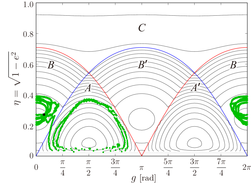
Figure 25: The equi-potential contours and numerical trajectories of the comet 122P/de Vico under the CR3BP framework plotted on the $(g,\eta)$ plane. The comet has the parameters of $(\alpha^{\prime},k^{2})\sim(0.295,0.000437)$. The green dots are the trajectories of this comet obtained through direct numerical integration of the equations of motion where we assume Jupiter on a circular orbit with the current semimajor axis and the current mass to be the perturbing body. As for the numerical integration, the nominal stepsize is 4 days, and the total integration time is 5 million years with a data output interval of 500 years. The initial starting point of the numerical integration is shown as a filled black square at $(g,\eta)=(0.0746\pi,0.271)$. The red and the blue curves are topologically equivalent to the red and the blue partial circles presented on the $(e\cos g,e\sin g)$ plane, such as in Fig. 24. The black dashed line near the bottom of the plot implies the upper boundary of the perturbed body’s eccentricity, equivalent to the black dashed circles presented on the $(e\cos g,e\sin g)$ plane, such as in Fig. 24. The red and the blue curves divide the plane into five domains which correspond to the domains $A$, $A^{\prime}$, $B$, $B^{\prime}$, and $C$ designated in Fig. 11.

As far as we are aware, currently the modern standard of the secular dynamical theory that can deal with orbit intersection of this kind is the work of Gronchi and Milani (1998, 1999). Some numerical demonstrations had existed before their work, but just for several special cases (e.g. Quinn et al., 1990; Bailey et al., 1992). Gronchi and Milani (1998) showed that it is possible to define a generalized averaged equation of motion even for a planet-crossing asteroid with singularities. They actually obtained generalized solutions that are unique and piecewise smooth with the help of an approximation proposed by Wetherill (1967) and the method of Kantorovich of extraction of singularities (e.g. Demidovich and Maron, 1966). Following this achievement, Gronchi and Milani (1999) proved that there is a stable region of orbits of the perturbed body for any values of $a$ and $k^{2}$ of an asteroid (or comet) and for any number of perturbing bodies with planar and circular orbits. While von Zeipel tried to obtain an expression of the disturbing function in each of the separated domains $A$, $B$, $C$, $\cdots$ in Fig. 11, Gronchi and Milani’s approach is to obtain an expression of the disturbing function that is common to all the regions. Although it is out of the scope of this monograph, it would be interesting to quantitatively compare their theory with von Zeipel’s to examine their difference and similarity in detail.

5.8.1 Motion of 1P/Halley

In the process of portraying their theoretical framework, Gronchi and Milani (1999, their Fig. 6 on p. 934) took one of the most famous comets—1P/Halley—as an example, and discussed its motion under the perturbation from major planets. According to one of their equi-potential diagrams (the bottom right panel in their Fig. 6), the motion of a 1P/Halley-like object has a stable equilibrium point around $g=\frac{\pi}{2}$ with a large eccentricity, although its equi-potential surface is irregularly shaped due to the lines of orbit intersection with major planets. Here, we want readers to recall that von Zeipel also carried out a quantitative demonstration on the secular motion of 1P/Halley earlier in his Section Z21 (see p. 5.6.3 of this monograph). Let us cite von Zeipel’s words about it:

“It might be interesting to apply the results of the previous issue to a case in the nature,” (p. Z395).

Note that “the results of the previous issue” indicates his theoretical development on the doubly averaged inner CR3BP (where $\alpha<1$, as we have seen in his Sections Z16–Z20).

von Zeipel begins his Section Z21 with a calculation of 1P/Halley’s eccentricity at one of its stationary points, $e_{0.2}$, using its orbital elements known at that time. He used the CR3BP framework including Jupiter as the perturbing planet on a circular orbit. He estimates 1P/Halley’s semimajor axis as $a=17.9676$ au according to Galle (1894), saying:

“The semi-major axis of the orbit of this comet is

17.9676.

This is the average distance [obtained from] all the apparitions of the comet from 1378 until 1835. (See J. G. Galle, List of elements of the previously calculated comets.) Choosing the semimajor axis of the orbit of Jupiter as unit length, we thus obtain

$$\alpha=17.9676:5.202800=3.45345.$$

” (p. Z395)

For calculating $k$ and $k^{\prime}$ of 1P/Halley, von Zeipel used its osculating orbital elements known at that time published in Galle (1894, pp. 50–51) and Rosenberger (1835a, b). They are tabulated on an unnumbered table on p. Z395 as

$$g =110^{\circ}37^{\prime}59^{\prime\prime},$$ (379)

$$h =55^{\circ}9^{\prime}47^{\prime\prime},$$

$$I =162^{\circ}14^{\prime}43^{\prime\prime},$$

$$e =0.96738879,$$

with a notice of “equinox through 1835 November 15.94542 t. m. of Paris.” von Zeipel converts these orbital elements into those on the solar system invariable plane, saying:

“By comparing the elements at the invariable plane of the solar system and by taking the value of the acute angle for the inclination, we obtained

$$I=18^{\circ}47^{\prime}44^{\prime\prime},\quad g=114^{\circ}27^{\prime}26^{\prime\prime}.$$

We see that $g$ is not very distant from $90^{\circ}$.

[From] the values indicated for $e$ and $I$, we give, for $k$ and $k^{\prime}$, the numbers as follows

$$k=\sqrt{1-e^{2}}\cos I =0.239789,$$

$$k^{\prime}=\sqrt{1-k^{2}} =0.970825,$$

” (p. Z396)

von Zeipel then moves on to the calculation of 1P/Halley’s $e_{0.2}$. For this purpose he did not use his own approximation formula presented as Eq. (Z94-313). Instead, he resorted to a numerical quadrature of $R$ along the axis of $g=\frac{\pi}{2}$. We literally cite von Zeipel’s words:

“Since $k$ is not very small, we have not employed the development (Z94) to calculate $e_{0.2}$. We have preferred to determine this quantity by calculating, by means of mechanical quadrature, a certain number of values of the function $R$ on the axis, where $g=\frac{\pi}{2}$. The value of $e$, which renders $R=$ minimum, is the sought value of $e_{0.2}$.

In these calculations, we used the formulas (Z48), (Z51) and (Z53). The field of integration was divided by $10^{\circ}$ to $10^{\circ}$. To calculate the complete elliptical of the first kind, the tables of Legendre were employed.” (p. Z396)

The resulting values of $e$ and $R$ are tabulated on an unnumbered table on p. Z396. From the tabulated values, von Zeipel draws the following conclusion:

“These numbers are found by means of interpolation calculations that

$$e_{0.2}=0.9537.$$

It is therefore a value very close to the actual eccentricity of the orbit of Halley’s comet.” (p. Z396)

Figure 26: A visualization of von Zeipel’s unnumbered table on p. Z396 that shows the dependence of comet 1P/Halley’s $R$ on its eccentricity $e$ along the axis of $g=\frac{\pi}{2}$. We simply connected the filled black circles (von Zeipel’s tabulated values) by straight line segments.

Instead of transcribing von Zeipel’s table, we have made a visual plot of the numbers tabulated in this table on an $(e,R)$ diagram (Fig. 26). We see a local minimum of $R$ in this figure, and the eccentricity value at that place seems to match what von Zeipel estimated as $e_{0.2}$ above (0.9537). Although he did not explicitly state this, we guess that von Zeipel wanted to claim that 1P/Halley’s argument of perihelion is currently located in the libration area centered at $(e,g)=(e_{0.2},\frac{\pi}{2})$. As a more straightforward demonstration, we carried out a set of numerical quadrature and direct numerical integration of the equations of motion of this comet, and drew the result on the $(g,\eta)$ plane. We placed Jupiter on a circular orbit with the current semimajor axis and the current mass as the perturbing body. The result is shown in Fig. 27. Under the CR3BP framework, we see that 1P/Halley’s $g$ librates at $g=\frac{\pi}{2}$ as von Zeipel predicted. In addition, the eccentricity value at the libration center that our calculation indicates (the small magenta triangle in Fig. 27) seems almost the same as what he calculated ($e=0.9537$, or $\eta\sim 0.301$). Here again, we believe that the accuracy of von Zeipel’s theory is confirmed.

Readers should be aware that, unlike 122P/de Vico, 1P/Halley is not in the state of “rings of a chain” with the perturber (Jupiter) in this dynamical setting. As the pericenter of this comet is inside the perturber’s orbit, and as the apocenter of this comet is outside the perturber’s orbit, it apparently seems that the orbit of this comet is located across the line of orbit intersection. However as seen in Fig. 27, the motion of this comet is confined in the domain $A$ defined in Fig. 11 with its argument of perihelion $g$ librating around $\frac{\pi}{2}$. Therefore its orbit does not make a “chain” with the perturber’s orbit. For a perturbed body’s orbit to compose a ring of a chain with perturber’s orbit, the perturbed body’s motion must be confined in the domain $B$ or $B^{\prime}$ with its argument of perihelion $g$ librating around $0$ or $\pi$.

Note also that our numerical result shown in Fig. 27 is just a numerical demonstration for confirming the validity and accuracy of von Zeipel’s theoretical estimate on 1P/Halley’s motion. In the actual solar system, close encounters with major planets frequently change this comet’s orbital elements, and its trajectory cannot remain regular. Even in the CR3BP approximation that we used to draw Fig. 27 we see an irregular oscillation in its trajectory, and this comet could not stay in the libration area centered at $g=\frac{\pi}{2}$ for more than one million years. Hence, it is easy to imagine that the actual motion of 1P/Halley in the actual solar system is much more complicated and irregular. This has been demonstrated by many previous studies (e.g. Chirikov and Vecheslavov, 1989; Lohinger et al., 1995; Bailey and Emel’yanenko, 1996; Muñoz-Gutiérrez et al., 2015; Boekholt et al., 2016). It is worth noting that Kozai (1979, his Fig. 4 in p. 234) analyzed 1P/Halley’s orbital motion through an equi-potential diagram, assuming four giant planets (Jupiter, Saturn, Neptune, and Uranus) as perturbers on circular orbits.

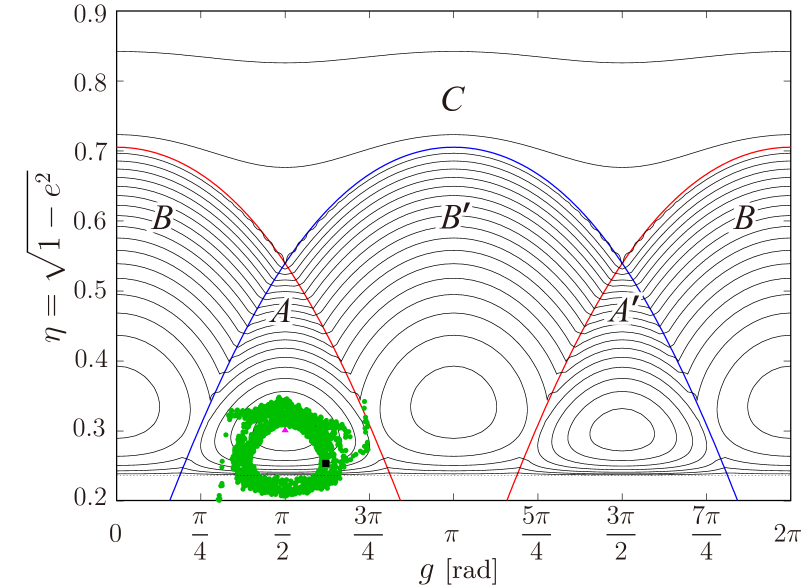
Figure 27: The equi-potential contours and numerical trajectories of the comet 1P/Halley under the CR3BP framework plotted on the $(g,\eta)$ plane. The comet has the parameters of $(\alpha^{\prime},k^{2})\sim(0.292,0.0558)$. The green dots are the trajectories of this comet obtained through direct numerical integration of the equations of motion where we assume Jupiter on a circular orbit with the current semimajor axis and the current mass to be the perturbing body. As for the numerical integration, the nominal stepsize is 1 day, and the total integration time is 1 million years with a data output interval of 500 years. The initial starting point of the numerical integration is shown as a filled black square at $(g,\eta)=(0.621\pi,0.254)$. We also plotted 1P/Halley’s $e_{0.2}$ value that von Zeipel calculated as the magenta filled triangle at $(g,\eta)=(\frac{\pi}{2},0.301)$ based on his estimate, $e_{0.2}=0.9537$. The meanings of the red and the blue curves, that of the black dashed line near the bottom, and the designation of the domains $A$, $A^{\prime}$, $B$, $B^{\prime}$, and $C$, are all common to those of Fig. 25. Note that the range of the vertical axis $(\eta)$ is narrower here than in Fig. 25. This is because 1P/Halley’s eccentricity is smaller than de 122P/Vico.

5.9 Some other extensions

The last section in von Zeipel’s Chapter IV (Section Z25), as well as his last chapter (Chapter V, Sections Z26–Z28), are both short. They are devoted to describing some other extensions of his theory.

5.9.1 Secular motion near the $e=k^{\prime}$ circle

Section Z25 is about a treatment of the doubly averaged motion of a perturbed body near the outer boundary of the $(e\cos g,e\sin g)$ plane; in other words, near the circle $e=k^{\prime}$. von Zeipel had mentioned this issue once in Section Z15 in his Chapter III in a general form (see p. 12 of this monograph). His discussion in Section Z25 eventually goes toward a statement at the end of this section (pp. Z414–415. We cite it later on p. 5.9.1) that, there exists a stable motion of perturbed body with $e\sim k^{\prime}$ on nearly a planar orbit. Below, let us quickly follow von Zeipel’s argument.

As we have seen, perturbed body’s inclination $I$ becomes small when its eccentricity $e$ approaches its largest value $(k^{\prime})$ in the doubly averaged CR3BP. This is due to the conservation of the quantity $k^{2}=\left(1-e^{2}\right)\cos^{2}I$. In order to deal with the motion of perturbed bodies with large $e$ and small $I$, von Zeipel brings up a different set of variables, $(\xi^{\prime},\eta^{\prime})$. Actually, he had already defined them in Section Z3 (his Chapter I, pp. Z349–Z350. See also p. Z06-202 of this monograph). See Eqs. (196) and (197) in this monograph for the definitions of $\xi^{\prime},\eta^{\prime}$ as well as those of $x^{\prime}_{1},x^{\prime}_{2},x^{\prime}_{3},y^{\prime}_{1},y^{\prime}_{2},y^{\prime}_{3}$. He first mentions the fact that the motion of the perturbed body near the outer boundary $e=k^{\prime}$ on the $(e\cos g,e\sin g)$ plane is translated into the motion around the origin $(0,0)$ on the $(\xi^{\prime},\eta^{\prime})$ plane. At the same time, von Zeipel reminds readers of the fact that the outer boundary $e=k^{\prime}$ on the $(e\cos g,e\sin g)$ plane behaves like a local maximum of the doubly averaged disturbing function $R$, particularly when $\alpha$ is small (see p. 265 of this monograph) or when $\alpha^{\prime}$ is small (see p. 5.7.2 of this monograph). He came to the conclusion that on the $(\xi^{\prime},\eta^{\prime})$ plane, the origin $(0,0)$ becomes a local maximum. Let us cite his original description about this:

“By studying the function $R$ for small values of $\alpha$ in no. Z16 and for small values of $\alpha^{\prime}$ at no. Z22, we have already remarked that, in both cases, the function $R$ increases if, $g$ remaining constant, the eccentricity $e$ increase toward the value $k^{\prime}$. The formula (Z42) shows that the inclination $I$ decreases toward zero when the eccentricity $e$ increases toward $k^{\prime}$. For values of $e$ close to $k^{\prime}$, it is therefore advantageous to introduce the variables of no. Z3. Among the variables $\xi^{\prime}$, $\eta^{\prime}$ of this no. Z3 and Keplerian variables, we obviously have the following relations

$${\xi^{\prime}}^{2}+{\eta^{\prime}}^{2} =2\sqrt{a}\sqrt{1-e^{2}}-2\sqrt{a}\sqrt{1-e^{2}}\cos I$$

$$=2\sqrt{a}\left(\sqrt{1-e^{2}}-k\right)$$

$$\eta^{\prime}:\xi^{\prime}=\tan g.$$

Therefore if, $g$ remaining constant, the eccentricity $e$ increases towards $k^{\prime}$, the corresponding point $\xi^{\prime}$, $\eta^{\prime}$ approaches the origin on a straight line.

It is therefore necessary to conclude that the function $R$, regarded as a function of variables $\xi^{\prime}$ and $\eta^{\prime}$ of no. Z3, has a maximum value at point $\xi^{\prime}=\eta^{\prime}=0$, if $\alpha$ is small enough or if $\alpha^{\prime}$ is small enough.” (p. Z413)

Note that $\eta^{\prime}:\xi^{\prime}$ means $\frac{\eta^{\prime}}{\xi^{\prime}}$ in the above.

von Zeipel then reminds readers of the condition for $R$ to be holomorphic (regular) over the entire region of $e\leq k^{\prime}$. This condition was already presented around Figs. Z1–Z5 on his p. Z369 (see Fig. 11 of this monograph, Eq. (227), and the discussions presented on pp. 5.5–5.5), but von Zeipel repeats it again here. Let us cite his words:

“We already know that $R$ is holomorphic in the neighborhood of $\xi^{\prime}=\eta^{\prime}=0$ as soon as

$$0<\alpha<\frac{1}{1+k^{\prime}}$$ (Z136-379)

or else

$$0<\alpha^{\prime}<1-k^{\prime},$$

(see Chapter III).” (p. Z413)

The first inequality of Eq. (Z136-379) corresponds to the circumstance that is depicted in Fig. 11a for the inner problem. The second inequality corresponds to the circumstance depicted in Fig. 11e for the outer problem.

Now, von Zeipel assumes that $R$ can be Taylor-expanded using ${\xi^{\prime}}^{2}$ and ${\eta^{\prime}}^{2}$ around the origin $(\xi^{\prime},\eta^{\prime})=(0,0)$, similar to the case when he expanded $R$ using $x^{2}=e^{2}\cos^{2}g$ and $y^{2}=e^{2}\sin^{2}g$ (see Eq. (Z77-253) or Eq. (Z99-326)). Let us cite his words again:

“Then, given the properties of symmetry of the disturbing function exhibited at no. Z4, it is necessary that $R$ is of the form

$$R=R^{\prime\prime}_{0.0}+R^{\prime\prime}_{2.0}{\xi^{\prime}}^{2}+R^{\prime\prime}_{0.2}{\eta^{\prime}}^{2}+\cdots.$$

From what has been said earlier, the inequalities

$$R^{\prime\prime}_{2.0}<0,\quad R^{\prime\prime}_{0.2}<0$$ (Z137-380)

exist as soon as, $k^{\prime}$ having been arbitrarily fixed but $<1$, we choose $\alpha$ or $\alpha^{\prime}$ small enough.” (p. Z413)

So far, von Zeipel’s statement has been about the case when $\alpha$ or $\alpha^{\prime}$ ($a$ or $a^{\prime}$ in his notation) is small. Then, would the two inequalities in Eq. (Z137-380) both hold true even when $\alpha$ (or $\alpha^{\prime}$) is not small? He questions this issue right after the previously quoted part:

“One may wonder if these inequalities [in Eq. (Z137-380)] always take place at the same time as one or other of the inequalities [in Eq.] (Z136-379).” (p. Z414)

To answer to this question, von Zeipel first considers the second inequality of Eq. (Z137-380), $R^{\prime\prime}_{0.2}<0$. Although we do not reproduce his specific calculations, in the end he concludes that $R^{\prime\prime}_{0.2}<0$ is always satisfied if either of the inequalities in Eq. (Z136-379) is satisfied, i.e. in the cases of Fig. 11a or Fig. 11e. Note that von Zeipel develops this consideration (on p. Z414) without showing the actual function form of $R({\xi^{\prime}}^{2},{\eta^{\prime}}^{2})$.

As for the first inequality of Eq. (Z137-380), $R^{\prime\prime}_{2.0}<0$, von Zeipel admits the difficulty of its proof when $\alpha$ or $\alpha^{\prime}$ is not small. Instead, he considers this inequality from its dynamical aspect. Here is how he describes his thought:

“It seems to be more difficult to rigorously discuss the sign of the coefficient $R^{\prime\prime}_{2.0}$ when $\alpha$ or $\alpha^{\prime}$ is no longer a relatively small quantity. But, see what would happen if the coefficient $R^{\prime\prime}_{2.0}$ could be positive, given one or other of the inequalities (Z136). Then the function $R$ has a minimaxima value at the point $\xi^{\prime}=\eta^{\prime}=0$. As a result, an orbit infinitely less inclined to the orbit of the disturbing planet and [yet] can never meet the orbit of this planet, could, by the effect of secular perturbations, obtain a finite inclination. It seems very unlikely. I therefore thought that it would probably be useless to examine the sign of the coefficient $R^{\prime\prime}_{2.0}$ by means of numerical calculations [that would be] inevitably quite long.” (p. Z414)

From the above considerations, at the end of Section Z25 von Zeipel makes a prediction on the existence of a class of cometary orbits. His words are as follows:

“It must be concluded from these studies and those of no. Z12 that there exist orbits of comet[s] in stable motion, whose inclinations are small, and for which the distance from the perihelion to the node possesses a positive mean motion (of the value $+\sigma$ from no. Z7). In these orbits the eccentricity is approximately constant $(=k^{\prime})$ as well as the semi-major axis. Finally, the nodes rotate in the opposite direction to the motion of the comet. Among these orbits, two classes are distinguished. In one [of them], the two nodes are located at the inside of the orbit of the disturbing planet, [and] in the other, the nodes are located, on the contrary, outside the orbit [of the disturbing planet].” (pp. Z414–Z415)

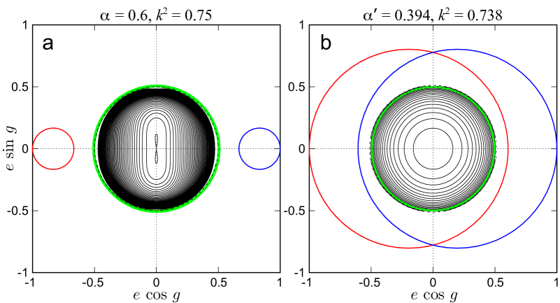
Figure 28: The equi-potential contours and numerical trajectories of perturbed bodies in two CR3BP systems whose eccentricities are close to their maximum, $k^{\prime}$. a: A fictitious body in an inner CR3BP system whose $\alpha=0.6$ and $k^{2}=0.75$. This means $k^{\prime}=\sqrt{1-k^{2}}=0.5$. The ratio of the perturber’s mass and the central mass is $9.5479194\times 10^{-5}$ which is close to $\frac{1}{10}$ of the mass ratio of Jupiter and the Sun. This system models a main belt asteroid orbiting inside Jupiter’s orbit. In this system, the perturbed body’s initial inclination is zero because $e=k^{\prime}$ is satisfied at the beginning. Thus its inclination remains zero (i.e. the planar orbit) throughout the calculation period because both the perturbed body’s orbit and the perturbing body’s orbit stay in the same plane. b: A fictitious body in an outer CR3BP system whose $\alpha^{\prime}=0.394$ and $k^{2}=0.733$. This means $k^{\prime}=\sqrt{1-k^{2}}\sim 0.516$. The ratio of the perturber’s mass and the central mass is the same as in the panel a. This system models a TNO orbiting outside Neptune’s orbit. In fact, the perturbed body in the system b is a proxy of an actual TNO, 2000 PH₃₀ whose orbital elements are $a=77.07718637$ au, $e=0.50203455$, and $I=8^{\circ}.048740$ according to astorb.dat provided by Lowell Observatory as of September 28, 2018 (see Supplementary Information 3 for its specific website). The value $\alpha^{\prime}=0.394$ adopted here is close to the semimajor axis ratio between Neptune and this object. In both the panels, the green dots near the outer boundary $(e=k^{\prime})$ indicate the trajectories of perturbed bodies obtained through direct numerical integration of the equations of motion. Parameters for the numerical integration are common to both a and b: the nominal stepsize is 4 days, the total integration time is 8 million years with a data output interval of 500 years. The meanings of the red and the blue circles, as well as the black dashed circles near the outer boundaries, are common to those in Fig. 25 and in Fig. 27. As usual, equi-potential contours of the perturbed body obtained through the numerical quadrature defined by Eq. (K09-53) are drawn in the black solid lines in both panels.

For confirming von Zeipel’s statement and prediction described above, particularly when $\alpha$ or $\alpha^{\prime}$ is not small, we carried out direct numerical integration of the equations of motion of two hypothetical perturbed bodies that are in the above category. One of them composes an inner CR3BP $(\alpha=0.6)$, and the other composes an outer CR3BP $(\alpha^{\prime}=0.394)$. The numerical results are presented in Fig. 28 together with the equi-potential contours for these objects obtained through the numerical quadrature defined by Eq. (K09-53). Note that in Fig. 28, we chose the conventional coordinates $(x,y)=(e\cos g,e\sin g)$ in this monograph, not $(\xi^{\prime},\eta^{\prime})$. This is for emphasizing how close the actual trajectories of the perturbed bodies (colored in green) are from their maximum eccentricity boundaries, $e=k^{\prime}$. If we use the coordinates $(\xi^{\prime},\eta^{\prime})$, all the numerical trajectories would concentrate on the vicinity of the origin $(0,0)$ of the plane, and would be very hard to distinguish.

By looking at Fig. 28, we can say that our numerical calculation reproduces well the orbital characteristics of the perturbed bodies that von Zeipel described. In both the panels a (the inner case) and b (the outer case), the perturbed body’s motion is stable for a long time with a large, nearly constant eccentricity $(e\sim k^{\prime})$ and a small, nearly constant inclination. The argument of pericenter $g$ circulates. Therefore we can conclude that von Zeipel’s prediction above (the possible existence of a stable motion of a perturbed body with a large, nearly constant eccentricity on nearly a planar orbit with the circulating argument of pericenter) is correct, even when $\alpha$ or $\alpha^{\prime}$ is as large as that shown in Fig. 28.

In the actual solar system, there is a category of small objects that possesses the characteristics that von Zeipel mentioned above. For example, as pointed out in the caption of Fig. 28, the perturbed body used in the system b is a proxy of an actual TNO (transneptunian object), 2000 PH₃₀. In the system b, we placed a Neptune-like planet on a circular orbit as the perturbing body so that they make an outer CR3BP. Therefore the value $\alpha^{\prime}=0.394$ adopted here is close to the semimajor axis ratio between Neptune and 2000 PH₃₀. This object has the parameter $k^{2}\sim 0.733$, therefore $k^{\prime}=\sqrt{1-k^{2}}\sim 0.516$. Hence the ratio between $e$ and $k^{\prime}$ of the perturbed body is quite large: $\frac{e}{k^{\prime}}>0.972$. This indicates that this object’s eccentricity is very close to the theoretical maximum in the CR3BP framework.

TNOs that possess both a large semimajor axis and a large eccentricity are collectively called the scattered TNOs (e.g. Gladman et al., 2008; Gomes et al., 2008; Lykawka and Mukai, 2007a, b; Lykawka and Mukai, 2008; Lan and Malhotra, 2019). Since many of the scattered TNOs have a much larger inclination than 2000 PH₃₀, this object may perhaps be an exception among this group. However, it is still interesting to know that there is at least one transneptunian object that fulfills von Zeipel’s prediction, and possibly many more. If we dare define this as von Zeipel’s “unintentional prediction” of a class of TNOs, we could say that it was achieved more than 30 years before Kenneth Edgeworth’s prediction of a small body population beyond Neptune’s orbit (Edgeworth, 1943, 1949). The number of objects in this category will surely increase along with the progress of ongoing and future observational surveys (e.g. LSST Science Collaboration, 2009; Yoshida et al., 2011; Bannister et al., 2016), which will further illuminate the foresight of von Zeipel on this subject. See p. 6.5 for a further discussion on this subject.

5.9.2 Two or more perturbers

von Zeipel’s final chapter is very short, entitled “Chapitre V. Généralisations. Applications aux orbites instables,” and includes four sections (Z26–Z29) over just four pages. This chapter is about a generalization of von Zeipel’s theory in order to incorporate $N$ perturbing planets $(N\geq 2)$, assuming that their eccentricities and inclinations are so small that we can ignore them. Although it may be practically a useful extension for actual problems in solar system dynamics, we think von Zeipel’s descriptions in this chapter are too short to accomplish his original intention. It is also hard for us to confirm the validity or accuracy of his discussion just from the description he put in this chapter. Therefore, what follows is our own interpretation of what he intended to claim.

Let us begin by telling readers an incidental but interesting fact. According to the ADS records as of September 15, 2019, the only citation of von Zeipel (1910) in the modern literature was made by Bailey and Emel’yanenko (1996). And, the reason why they cited von Zeipel’s work is due to the subject in his Chapter V. The description in Bailey and Emel’yanenko (1996) reads:

“It is well known that if $N_{P}$ planets are assumed to be on coplanar circular orbits, the problem of the motion of a small body under the influence of the secular part of the disturbing function is integrable (Zeipel 1910; Moiseev 1945; Kozai 1962; Vashkov’yak 1981a,b), and may be reduced to a description of the integrable curve in the $(e,\omega)$ plane.” (Bailey and Emel’yanenko, 1996, the left column on p. 1095, the beginning of Section 5)

From what we have seen, we learned that the addition to CR3BP of a perturbing planet orbiting on a planar and circular orbit $(e^{\prime}=I^{\prime}=0)$ would not increase the degrees of freedom after averaging, and the system would remain integrable. This principle would not be different even when $N$ perturbing planets are included. The only issue would be how to specifically calculate the secular perturbation from the multiple perturbers. At the beginning of his Section Z26, von Zeipel states the issue as follows:

“In what preceded, we have assumed that there was one disturbing planet, and that the eccentricity of its orbit was zero. But it is possible to generalize [this study] by assuming that the number of disturbing planets is any $N$ and that their masses as well as the eccentricities and inclinations of their orbits are small.” (p. Z415)

After some preparation such as extending the variables and secular equations of motion for the $N$-perturber system, von Zeipel claims that the doubly averaged disturbing function $R$ that contains perturbations from multiple perturbing planets is composed by a sum of multiple disturbing functions. Let us cite his original description:

“$\ldots$ By neglecting these first modules, which is equivalent to neglecting the eccentricities and the inclinations, the function $R$ has the form

$$R=R^{(0)}=\sum_{i=1}^{N}\frac{\beta_{i}}{a_{i}}R_{i}.$$ (Z140-381)

The $\beta_{i}$ are the masses of the planets, the mass of Jupiter being chosen as the unit; the $a_{i}$ are the zero-order secular parts of the semimajor axes of the orbits of the planets; finally $R_{i}$ are obtained by the formula (Z44) by putting only

$$\frac{a}{a_{i}}\mbox{ instead of }a.$$

” (p. Z416)

As a result of his consideration and approximation, it turns out that we can again use Eq. (Z12-219) as the equations of motion of the multiple perturber system. The only difference from the single perturber system is that we would have to replace $R$ in Eq. (Z12-219) for $R^{(0)}$ in Eq. (Z140-381). Consequently, it would be possible to construct the Lindstedt series if $R^{(0)}$ possesses the local extremum.

In Section Z27 von Zeipel studies the characteristics of $R^{(0)}$ in Eq. (Z140-381), and tries to locate its local extremums if any. He first mentions the fact that, when there are $N$ perturbers, the phase space $(x,y)=(e\cos g,e\sin g)$ is divided into pieces by $N$ pairs of circles. The $N$ pairs of circles are expressed by the following equations:

$$\left(x\pm\frac{a_{i}}{2a}\right)^{2}+y^{2}=\left(1-\frac{a_{i}}{2a}\right)^{2}\quad i=1,2,\cdots N.$$ (Z141-382)

This is topologically different from the single perturber system where the phase space is divided just by a pair of circles expressed as Eq. (Z45-227).

Although von Zeipel did not show any figures that demonstrate the phase space division by $N$ perturbers represented by Eq. (Z141-382), Gronchi and Milani’s (1999) Fig. 1 on their p. 929 is an exact example of how the multiple circles (Z141-382) divide the phase space. von Zeipel insists that each of the divided domains has a corresponding disturbing function. Literary citing his words:

“By means of these circles, the domain (Z46) will be divided into a certain number of parts $(D_{j})$. In any of these domains $(D_{j})$ [there] corresponds to a function $R_{j}$, holomorphic in this domain and on its boundaries (except the circle $e=k^{\prime}$), and giving the value of $R^{(0)}$ in this domain.” (p. Z416)

von Zeipel continues his discussion in the subsequent section (Z28). He particularly focuses on the search for, and evaluation of, local extremums of $R^{(0)}$ in each of the divided domains. He begins the study in this section with a description of the behavior of $R^{(0)}$ at the coordinate origin, $(\xi,\eta)=(0,0)$. Citing his words:

“Now consider the maximum and minimum values of the function $R^{(0)}$.

At the origin $\xi=\eta=0$, the function $R^{(0)}$ can be minima, maxima or minimaxima according to the values of parameters $a$ and $k$. It is obvious that $R^{(0)}$ is always minimum at the origin if $k^{2}$ is close enough to unity.” (p. Z417)

In the analogy of what von Zeipel has demonstrated over the past chapters, we find the above statement correct. Note that the variables $(\xi,\eta)$ were defined earlier in his Chapter I (p. Z349; see Eqs. (189) and (190)). If we use the ordinary Delaunay elements, they are expressed as follows:

$$\xi =\>\>\>\sqrt{2(L-G)}\cos g,$$ (384)

$$\eta =-\sqrt{2(L-G)}\sin g.$$ (385)

From the definitions in Eqs. (384) and (385), we anticipate that $R^{(0)}$’s behavior on the $(\xi,\eta)$ plane is topologically the same as that on the $(x,y)=(e\cos g,e\sin g)$ plane.

In the second and the third paragraphs of Section Z28, von Zeipel gives a description of a system where all the disturbing planets are located outside the perturbed body. This kind of system can be regarded as an extension of the inner CR3BP. We cite his description:

“Consider first the orbits where $a$ is smaller than the semimajor axis of the orbit of Jupiter. Given the dominant mass of this planet, it is clear, looking at the tables giving $R_{2.0}$, $R_{0.2}$, $R^{\prime}_{2.0}$ and $R^{\prime}_{0.2}$, that the function $R^{(0)}$ is minima at the origin $\xi=\eta=0$ if

$$k^{2}_{0.2}<k^{2}<1$$

and minimaxima if

$$0<k^{2}<k^{2}_{0.2}.$$

The proposition on the page Z390 and the remark on [the] revolution of planetary system of the page Z392 are still valid for the parts of the solar system at the interior of the orbit of Jupiter. Only, by the effect of other planets, the limit $I_{0.2}$ (of the page Z389) will be a little high.” (p. Z417)

Later in this monograph (p. 6.5) we will briefly state what we think he meant by “the remark on [the] revolution of planetary system of the page Z392”.

In von Zeipel’s above statement, the last sentence on the change of the limiting inclination $I_{0.2}$ “Only, by the effect of other planets, the limit $I_{0.2}$ (of the page Z389) will be a little high” draws our particular attention. Let us interpret it as follows. Consider a typical inner CR3BP system, Sun–asteroid–Jupiter. Then, the addition of yet another disturbing planet orbiting exterior to Jupiter’s orbit (such as Saturn) would change the shape of the total disturbing potential that the perturbed asteroid feels. It means that the condition for the equilibrium points to occur could be less easily achieved. Let us choose an asteroid with $\alpha=0.65$ as an example of perturbed body. According to our Fig. 15 (p. 15), its limiting inclination $I_{0.2}$ is roughly $27^{\circ}.6$ (equivalent to $k^{2}_{0.2}\sim 0.785$). Now, consider yet another disturbing planet orbiting exterior to Jupiter’s orbit. The $\alpha$ value of the perturbed asteroid with respect to this new, exterior perturber (referred to as $\alpha^{\rm e}$) would then become smaller than 0.65 (i.e. $\alpha^{\rm e}<\alpha$). This means that the limiting inclination with respect to the new exterior perturber (referred to as $I^{\rm e}_{0.2}$) would be larger than $I_{0.2}$. If we place the two perturbers (Jupiter and the exterior planet) at the same time in this system, the total perturbation from the two perturbers would be a combination of the two CR3BPs that have a limiting inclination of $I_{0.2}(\alpha)$ and $I^{\rm e}_{0.2}(\alpha^{\rm e})$, respectively. And, since $I^{\rm e}_{0.2}>I_{0.2}$, the resulting limiting inclination of the perturbed asteroid in the two perturber system would be larger than $I_{0.2}$. This is our interpretation of von Zeipel’s above sentence.

In the following paragraph of Section Z28, von Zeipel gives a description of a system where all the disturbing planets are located inside the orbit of the perturbed body. This kind of system can be regarded as an extension of the outer CR3BP. At the same time, he also considers a system where the orbit of the perturbed body is located just outside the orbit of one of the disturbing planets (so that the influence of other disturbing planets gets relatively smaller). His remarks about this are as follows:

“Consider then the values of $a$, which are larger than the semimajor axis of the orbit of Jupiter. If $a$ is between certain limits, especially if $a$ is larger than the semimajor axis of the orbit of the last planet (Neptune) or slightly larger than the semimajor axis of the orbit of Uranus, Saturn or Jupiter, then $R^{(0)}$ can be maximum for small values of $k^{2}$. Conversely, if $a$ is a bit smaller than the semimajor axis of the orbit of Saturn, $R^{(0)}$ is minimaximum for small values of $k^{2}$.” (p. Z417)

We already learned that, the doubly averaged disturbing function for the outer CR3BP takes a local maximum at the origin $(x,y)=(0,0)$ when $k^{2}$ is small enough (see Fig. 17 or Fig. 19 of this monograph). von Zeipel’s first conclusion in the above paragraph (“$\cdots$ if $a$ is larger than the semimajor axis of the orbit of the last planet (Neptune) $\cdots$ then $R^{(0)}$ can be maximum for small values of $k^{2}$”) seems consistent with this fact. On the other hand, the last sentence of the above paragraph (“Conversely, if $a$ is a bit smaller than the semimajor axis of the orbit of Saturn, $R^{(0)}$ is minimaximum for small values of $k^{2}$”) seems similar to the discussion that we had at the inner CR3BP where $R$ takes a saddle point at the origin $(0,0)$ when $k^{2}$ is small enough.

As a consequence of the above considerations, von Zeipel reaches a specific conjecture, and writes:

“We can conclude from this that, in the solar system, there may be orbits which are always not very eccentric and have inclinations close to $90^{\circ}$. These orbits may exist somewhat outside the orbit[s] of Jupiter, Saturn or Uranus. But above all, they might be outside the last planet of the system.” (p. Z417)

As we saw in Section 5.7 of this monograph about the doubly averaged outer CR3BP, this kind of orbit—not very eccentric, with a large inclination (if not nearly $90^{\circ}$), and located somewhat outside the outermost perturbing body—can stably exist if $k^{2}$ is small enough. An orbit of this kind would be confined near the origin $(0,0)$ of the $(e\cos g,e\sin g)$ plane. For example, the CR3BP systems employed in Figs. 23a and 23e with $(\alpha^{\prime},k^{2})=(0.6,0.2600)$ predict the existence of stable orbits of perturbed bodies whose inclination is nearly $60^{\circ}$ around the origin where $e=0$.

If we turn our attention to the actual solar system, we recognize a certain number of objects in this category—small $e$, large $I$, located somewhat outside the orbit of perturbing planets, and whose $k^{2}$ is small. We chose several small objects of this kind and listed them in Table 4. As seen in this table, we may want to classify the candidate objects in two categories. The first category comprises objects with very small $k^{2}$ and large inclination, but with moderate eccentricity. The ten objects in the upper part of Table 4 denoted as “small $k^{2}$” correspond to these. See the caption of Table 4 for details of our empirical determination criteria. The second category contains objects with a very small eccentricity, but with a mildly high inclination, therefore their $k^{2}$ is not so small. The six objects in the lower part of Table 4 denoted as “small $e$ and large $I$” correspond to these. Existence of these two orbital characteristics may imply something about how these objects were formed and how their orbits have been dynamically evolved. But here, let us just emphasize that a substantial number of small bodies in the actual solar system satisfy the orbital conditions that von Zeipel has depicted, at least partially. We believe this corroborates the correctness of his theory. These objects are either Centaurs or TNOs by definition, and their discoveries were made many decades later than von Zeipel’s era—Centaurs were not discovered until 1977 when (2060) Chiron was found, and TNOs were not discovered until 1992 when 1992 QB₁ was found, except for Pluto which was discovered in 1930. As the number of objects in these categories increases along with the progress of observational surveys, the validity of von Zeipel’s theory will be more rigorously verified and substantiated.

Table 4: Osculating orbital elements $a$, $e$, $I$ and the parameter $k^{2}$ of several small objects in the actual solar system that can match von Zeipel’s description in his Section Z28: Not very eccentric, with an inclination close to $90^{\circ}$, and located somewhat outside the orbit of perturbing planet. The data is taken from the file astorb.dat provided by Lowell Observatory as of September 28, 2018. We chose and put the objects into two categories. The objects in the first category are those with very small $k^{2}$ with a large inclination and moderate eccentricity. They are denoted as “small $k^{2}$” on the left-end of the table. Our empirical determination criteria for this category is $k^{2}<0.2$. The objects in the second category have a very small eccentricity but with a mildly high inclination; therefore their $k^{2}$ is not quite small (denoted as “small $e$ and large $I$”). Our determination criteria for this category is $e\lesssim 0.08$ and $I$ (or $\pi-I$) ranges from $40^{\circ}$ to $50^{\circ}$. The orbit type (Centaur or TNO) is based on the categorization by the JPL Small-Body Database Browser: Centaurs are defined as objects with orbits between Jupiter and Neptune $(5.5\>\mathrm{au}<a<30.1\>\mathrm{au})$, and TNOs are defined as objects with orbits outside Neptune $(a>30.1\>\mathrm{au})$. The ratio of the semimajor axes between each small object and its major perturbing planet (in the framework of the outer CR3BP) is denoted as $\alpha^{\prime}$. This is either $\alpha^{\prime}_{\mathrm{J}}=\frac{a_{\mathrm{J}}}{a}$, $\alpha^{\prime}_{\mathrm{S}}=\frac{a_{\mathrm{S}}}{a}$, $\alpha^{\prime}_{\mathrm{U}}=\frac{a_{\mathrm{U}}}{a}$, or $\alpha^{\prime}_{\mathrm{N}}=\frac{a_{\mathrm{N}}}{a}$, where $a_{\mathrm{J}}$, $a_{\mathrm{S}}$, $a_{\mathrm{U}}$, $a_{\mathrm{N}}$ are the semimajor axes of Jupiter, Saturn, Uranus and Neptune, respectively. Note that, for each small object, we just put the value of $\alpha^{\prime}$ for the closest perturbing planet. For example, we only showed the value of $\alpha^{\prime}=\alpha^{\prime}_{\mathrm{S}}=0.82219$ for 2008 YB₃, not $\alpha^{\prime}_{\mathrm{J}}$, $\alpha^{\prime}_{\mathrm{U}}$, or $\alpha^{\prime}_{\mathrm{N}}$. This is because Saturn’s orbit is closer to this object than any of the other three planetary orbits. Near the right-end of the table, “arc (d)” denotes the number of days spanned by the observational data arc for the object, and $n_{\mathrm{obs}}$ indicates the number of observations used to determine the orbital elements. We included these two columns to gauge the accuracy (or inaccuracy) of the orbit determination for each object. Here is a note on the symbol $(\ast 1)$ for the orbit type of 2015 KG₁₅₇: This object’s orbital elements have been determined from just twelve sets of observations $(n_{\mathrm{obs}}=12)$ spanning just two days $(\mathrm{arc}=2)$. Consequently, they contain a non-negligible amount of uncertainties. In fact, on the JPL Small-Body Database Browser its semimajor axis is denoted as $a=5.928588171390333\pm 2.3908$ au (as of November 14, 2018) which is slightly different from the value listed on astorb.dat, and its orbital type is categorized as Centaur. Similar uncertainties lie in the orbital elements of 2006 HU₁₂₂ and 2016 FM₅₉ whose observational arcs are short. Note also that some of the TNOs in the table may be in the category of resonant TNOs if their orbits are accurately determined. For example, 2014 XZ₄₀’s orbital location is similar to that of Plutinos (those in the 2:3 mean motion resonance with Neptune), and that of 2006 HU₁₂₂ is rather close to the 4:7 mean motion resonance with Neptune. We would need a long-term direct numerical integration for accurately characterizing their dynamical categorization. For a better understanding of what kind of orbits these objects actually have, in Supplementary Information 5 we put figures for the orbital diagrams of all the objects listed in this table.

	object	type	$a$ (au)	$e$	$I$ (deg)	$k^{2}$	$\alpha^{\prime}$	arc (d)	$n_{\mathrm{obs}}$
small $k^{2}$	outside Jupiter
	2015 KG157	$(\ast 1)$	5.39893316	0.42080926	72.904103	0.07112	0.96363 $(\alpha^{\prime}_{\mathrm{J}})$	2	12
	2007 VW266		5.44387890	0.39031355	108.310551	0.08366	0.95568 $(\alpha^{\prime}_{\mathrm{J}})$	38	59
	2010 CR140	Centaur	5.62365608	0.40883143	74.667719	0.05823	0.92513 $(\alpha^{\prime}_{\mathrm{J}})$	1418	43
	2012 YO6	Centaur	6.31511335	0.47807149	106.886748	0.06509	0.82383 $(\alpha^{\prime}_{\mathrm{J}})$	142	47
	2014 JJ57	Centaur	6.99082311	0.29313977	95.922691	0.00973	0.74420 $(\alpha^{\prime}_{\mathrm{J}})$	2815	30
	outside Saturn
	2008 YB3	Centaur	11.62121366	0.44058710	105.059221	0.05440	0.82219 $(\alpha^{\prime}_{\mathrm{S}})$	3236	502
	outside Uranus
	2011 MM4	Centaur	21.14652789	0.47287733	100.490295	0.02574	0.90882 $(\alpha^{\prime}_{\mathrm{U}})$	2552	144
	2007 BP102	Centaur	23.96197862	0.25905974	64.680786	0.17062	0.80204 $(\alpha^{\prime}_{\mathrm{U}})$	3396	51
	outside Neptune
	2011 KT19	TNO	35.58572066	0.33046594	110.102428	0.10523	0.84614 $(\alpha^{\prime}_{\mathrm{N}})$	1779	132
	2008 KV42	TNO	41.58639205	0.49226472	103.398712	0.04068	0.72404 $(\alpha^{\prime}_{\mathrm{N}})$	3610	55
small $e$ and large $I$	outside Jupiter
	2016 LN8	Centaur	5.76477817	0.04542763	43.360457	0.52751	0.90248 $(\alpha^{\prime}_{\mathrm{J}})$	6290	94
	outside Neptune
	2014 XZ40	TNO	39.65156553	0.05013667	44.564654	0.50632	0.75937 $(\alpha^{\prime}_{\mathrm{N}})$	77	10
	2013 SA87	TNO	41.67277625	0.07141871	40.868092	0.56895	0.72254 $(\alpha^{\prime}_{\mathrm{N}})$	1400	53
	2004 DF77	TNO	43.55225696	0.02231651	43.670818	0.52293	0.69136 $(\alpha^{\prime}_{\mathrm{N}})$	17	4
	2006 HU122	TNO	44.84803376	0.08128279	46.907861	0.46364	0.67139 $(\alpha^{\prime}_{\mathrm{N}})$	1	3
	2016 FM59	TNO	45.12950220	0.05981495	131.522580	0.43788	0.66720 $(\alpha^{\prime}_{\mathrm{N}})$	3	9

The next section (Z29) that closes von Zeipel’s work (1910) is composed of a very brief consideration on the secular motion of a comet, 2P/Encke. This section seems to be an exposition of his theory on the doubly averaged restricted systems with more than one perturbing body stated in this chapter. However the description in this section is too concise, and it does not seem to contain much quantitative material that we should deal with in this monograph. Therefore we do not go into the contents of this section.

6 Summary and Discussion

Since we are in the final part of this monograph, we bring up several issues to conclude our study. In Sections 6.1, 6.2, and 6.3, we try to organize and compare the achievements presented in the works of Kozai, Lidov, and von Zeipel. After that, in Section 6.4 we introduce von Zeipel’s earlier publications that can be regarded as a preparatory step toward his 1910 paper. Finally in Sections 6.5 and 6.6, we express our opinion as to how the secular dynamical effect discussed in this monograph should be referred to, in comparison with several historical examples.

Table 5: A comparison of the achievements shown in Kozai’s, Lidov’s, and von Zeipel’s work. Some symbols have superscript numbers that have the following meanings: 1: There are some descriptions, but they are very terse and do not seem complete. 2: Mentioned in Lidov (1963b, c) just for a limited case when $i=\frac{\pi}{2}$. 3: Described in Lidov (1963b, c) for a limited case. 4: Orbital variation of the satellites of Uranus is discussed in Lidov (1963b, c). 5: Described in Lidov (1963b, c) briefly. 6: Drawn by hand, but topologically correct. 7: $I_{0}$ and $I_{0.2}$ of several asteroids such as (2) Pallas or (531) Zerlina are calculated and discussed. 8: Motions of 1P/Halley and 2P/Encke are quantitatively discussed. 9: Detailed mathematical exposition is presented, but without tables or figures. 10: Mathematical exposition is presented without tables or figures.

	Kozai	Lidov	von Zeipel
General features and treatment of CR3BP
Hamiltonian formalism	$\bigcirc$	—	$\bigcirc$
Gauss’s form of equations	—	$\bigcirc$	—
single averaging	—	$\bigcirc$	—
double averaging	$\bigcirc$	$\bigcirc$	$\bigcirc$
conservation of $\left(1-e^{2}\right)\cos^{2}i$	$\bigcirc$	$\bigcirc$	$\bigcirc$
conservation of total energy	$\bigcirc$	$\bigcirc$	$\bigcirc$
numerical quadrature	$\bigcirc$	—	$\bigcirc$
direct numerical integration	—	$\bigcirc$	—
Doubly averaged inner CR3BP
libration of $g$ around $\pm\frac{\pi}{2}$	$\bigcirc$	$\bigcirc$	$\bigcirc$
conservation of $c_{2}$-like variable	—	$\bigcirc$	—
solutions in special cases	$\bigtriangleup^{1}$	$\bigcirc$	—
time-dependent analytic solution	$\bigcirc$	$\bigtriangleup^{2}$	—
equi-potential contours	$\bigcirc$	$\bigtriangleup^{3}$	$\bigcirc^{6}$
treatment when $\alpha$ is not small	$\bigcirc$	—	$\bigcirc$
mention of actual objects	$\bigcirc$	$\bigtriangleup^{4}$	$\bigcirc^{7}$
oblateness of central mass	—	$\bigtriangleup^{5}$	—
Doubly averaged outer CR3BP
libration of $g$ around $\pm\frac{\pi}{2}$	—	—	$\bigcirc$
libration of $g$ around $0$ or $\pi$	—	—	$\bigcirc$
equi-potential contours	—	—	$\bigcirc^{6}$
treatment when $\alpha^{\prime}$ is not small	—	—	$\bigcirc$
mention of actual objects	—	—	$\bigcirc^{8}$
Other features and treatment
Treatment of orbit intersection	—	—	$\bigcirc^{9}$
Multiple perturbing bodies	—	—	$\bigtriangleup^{10}$

For comparing the works of the three authors, we have made a list of similarities and differences between the works of Kozai, Lidov, and von Zeipel in Table 5. In this table, the open circles $(\bigcirc)$ denote “achieved and clearly presented” by the work. The long hyphens (—) denote “not achieved or mentioned.” The open triangles $(\bigtriangleup)$ denote “partially achieved or just mentioned, or mentioned in relevant publications.” We admit that our evaluation for these three categories ($\bigcirc$, —, $\bigtriangleup$) are subjective, and sometimes ambiguous. For example, we graded “numerical integration of orbits” in Lidov’s work as $\bigcirc$, but it can be arguable whether or not the numerical integration presented in Lidov’s work is worth a discussion in the context of modern celestial mechanics.

6.1 Achievements of Kozai’s work

Kozai’s work has been recognized as a classic in this line of study. As we learned, he began with a general Hamiltonian formalism of the inner CR3BP, and derived the secular disturbing function through the double averaging procedure. Through the analysis of the doubly averaged disturbing function, Kozai showed the possibility of libration of the perturbed body’s argument of pericenter $g$ around $\pm\frac{\pi}{2}$ under a certain condition. He clarified the condition to be $\Theta=\left(1-e^{2}\right)\cos^{2}i<\frac{3}{5}$ at the quadrupole level approximation. As we have seen, Kozai’s $\Theta$ is equivalent to Lidov’s $c_{1}$ and von Zeipel’s $k^{2}$. Kozai did not mention any parameters equivalent to Lidov’s $c_{2}$ whose sign explicitly tells us whether or not the perturbed body’s argument of pericenter librates at the quadrupole level approximation.

One important accomplishment in Kozai’s work is that he employed diagrams with equi-potential contours of the doubly averaged disturbing function as a fundamental subject of discussion. Kozai’s aim of exploiting the equi-potential diagrams was to show the global structure of possible trajectories that the perturbed body draws, and to visually confirm the existence of equilibrium points. Using the equi-potential diagrams, Kozai found that the argument of perihelion $g$ of (1373) Cincinnati librates around $g=\frac{\pi}{2}$. It seems that Kozai reached this conclusion just from the topological pattern of the equi-potential contours and the initial location of this asteroid (Fig. K7 on p. K597), not following the time variation of its orbital elements. Nowadays we see this kind of equi-potential diagram ubiquitously in the literature, not only in CR3BP studies, but in other dynamical studies where a system’s degrees of freedom can be somehow reduced to unity. In this regard, Kozai was a pioneer.

For calculating the equi-potential contours, Kozai carried out the numerical quadrature defined by Eq. (K09-53). Kozai called the quadrature “numerical harmonic analysis” (p. K593, the left column, four lines below Eq. (K17). Also in the caption of his Fig. K1). It is not hard to imagine that carrying out numerical quadrature in the early 1960s was a formidable task when the use of high-speed digital computers was extremely limited. However, Kozai completed the numerical work using digital computers available in the United States while he was a long-term visiting scholar at Smithsonian Astrophysical Observatory, Cambridge, Massachusetts (Kozai 2017, personal communication). Although we have not confirmed if Kozai’s work is the very first one that quantitatively exploits equi-potential diagrams in celestial mechanics, we are convinced that Kozai was one of the first to recognize the importance and usefulness of the equi-potential contours in this line of study.

Incidentally, note that Shevchenko (2017, his Section 3.2.4 on p. 39) calls the equi-potential diagrams “the Lidov–Kozai diagram.” We do not agree with his opinion mainly because there is no such equi-potential contour plot in Lidov’s original paper (1961). There is an equi-potential diagram in his later papers (Lidov, 1963b, c) but it was just used for a special case. Moreover, as we have seen in this monograph, von Zeipel had already drawn this kind of equi-potential diagrams much earlier (see Figs. 11 and 13 in this monograph) even though they look somewhat schematic.

We should also recall that Kozai derived explicit expressions of high-order analytic expansions of the doubly averaged disturbing function for the inner CR3BP up to $O\left(\alpha^{8}\right)$, which is reproduced as Eq. (K23-70). This is not achieved in Lidov’s work or in von Zeipel’s work. Using Kozai’s analytic expansion, we can draw equi-potential curves of perturbed bodies accurately without going through numerical quadrature, even when $\alpha$ is not small.

Yet another unique achievement seen only in Kozai’s work is that he derived a time-dependent analytic solution for orbital elements as function of time by employing Weierstrass’s elliptic functions $\wp$ (see p. 3.5 of this monograph). The equi-potential trajectories calculated from the doubly averaged disturbing function show us the dynamical structure of perturbed bodies at a glance, but they do not give us information about their time variation, such as $e(t)$ or $g(t)$. Having the time-dependent analytic solution that Kozai constructed, we can calculate approximate time variation of perturbed body’s orbital elements, even though the approximation is limited to the quadrupole level.

6.1.1 Later developments

Kozai’s work has been checked, confirmed, and developed by numerous authors including Kozai himself since its publication in 1962. We can pick the following developments as for Kozai’s four remarks on future prospects that we mentioned in Section 3.8.

As for the issue (i) on the effect of perturber’s non-zero eccentricity $e^{\prime}$, its influence has turned out to be quite significant. It is now well known as the eccentric Lidov–Kozai (or Kozai–Lidov) oscillation (e.g. Naoz, 2016; Sidorenko, 2018). It can substantially change the long-term orbital motion of the perturbed body, sometimes invoking sudden orbital flips as we demonstrated in Fig. 4 (p. 4).

As for the issue (ii) on the incorporation of the indirect perturbation from other planets, Kozai himself succeeded in incorporating the effect of other planets by assuming that they have circular orbits (Kozai, 1979). This was possible because the inclusion of perturbers on planar and circular orbits would not increase the total degrees of freedom of the system after the averaging procedure. The same subject was studied by Vashkovjak (1976) and Vashkov’yak (1981c). Kozai’s method was followed, and used by many later studies (e.g. Nakai and Kinoshita, 1985; Ito and Tanikawa, 1999, 2001; Ito and Miyama, 2001).

As for the issue (iii) on the inclusion of planetary oblateness on the motion of satellites, Lidov (1963b, c) studied it shortly later than Kozai. Kozai extended his theory by himself by including the oblateness of central body such as $J_{2}$, $J_{3}$, and $J_{4}$ (Kozai, 1969b). Much later, Kinoshita and Nakai (1991) worked on the point that Kozai raised: Possible decrease and disappearance of the threshold value of perturbed body’s $\left(1-e^{2}\right)\cos^{2}i$ due to planetary oblateness. Kinoshita and Nakai quantitatively formulated the influence of Uranian $J_{2}$ on the secular motion of its fictitious satellites. They found that when the Uranian satellites are located inside the region where the perturbation caused by planetary oblateness is dominant, their argument of pericenter does not librate, and stationary points do not occur.

As for the issue (iv) on the motion of satellites for which the orbital period of the Sun may not be regarded as short, we presume that the subject is in the realm of the singly averaged three-body system such as Moiseev or Lidov dealt with. Although the single averaging procedure is not very popular now, mostly because they can be replaced for direct numerical integration in many cases, there is still a certain flow of studies along this line in modern celestial mechanics (e.g. Domingos et al., 2013; Elshaboury and Mostafa, 2013; Nie et al., 2019). There are even studies of singly averaged hyperbolic (Sorokovich, 1982) and parabolic (Mamedov, 1989) restricted three-body problems.

Efforts to obtain the time-dependent analytic solutions of perturbed body’s orbital elements in the doubly averaged CR3BP using elliptic functions, as Kozai demonstrated, has been continued and extended. However Weierstrass’s elliptic functions $\wp$ that Kozai employed are not used anymore in this respect. A major extension of this line of work was achieved by a pair of Japanese celestial mechanists, Hiroshi Kinoshita and Hiroshi Nakai, both of who worked close to Kozai. Kinoshita and Nakai (1991) succeeded in deriving an analytic solution for this problem using Jacobi’s elliptic function that can be used when the perturbed body’s $g$ circulates. Kinoshita and Nakai (1999) later gave another type of analytic solution expressed by Jacobi’s elliptic function that can be used when the perturbed body’s $g$ librates around $\frac{\pi}{2}$. Finally Kinoshita and Nakai (2007) reached a general analytic solution that can be used either when the perturbed body’s $g$ librates or when it circulates. We should note that Vashkov’yak (1999) had also reached a general solution of this kind independently, through a slightly different way, for the motion of distant satellites of Uranus.

So far, these analytic solutions are derived from the doubly averaged disturbing function of the inner CR3BP at the quadrupole level approximation, and their practical usefulness does not seem to be as significant as direct numerical integration. However, the way of deriving the time-dependent analytic solutions in these works seems to be inherited from dynamical studies of comets with very large perihelion distances under the galactic tide. More specifically speaking, the dynamical evolution of small bodies that compose the Oort Cloud (Oort, 1950, 1951) under the galactic tide has been often discussed and calculated using analytically obtained approximate solutions (e.g. Heisler and Tremaine, 1986; Fouchard et al., 2005; Higuchi et al., 2007). These works can be regarded as an extension of Kozai’s work. Note also that, in a small body system that is under the perturbation from the galactic tide, the quantity $\sqrt{1-e^{2}}\cos I_{\mathrm{g}}$ becomes constant after averaging over small body’s mean anomaly if we only take the vertical component of the galactic tide (where $I_{\mathrm{g}}$ denotes orbital inclination of the small body with respect to the galactic plane). This is due to the rotational invariance of the averaged galactic tidal potential around the normal of the galactic plane (e.g. Saillenfest et al., 2019). This point is similar to the doubly averaged CR3BP that we have considered in this monograph. Breiter and Ratajczak (2005, their p. 1222) presents a concise review of the historic development of this line of studies.

At the end of this subsection, we would like readers to pay attention to a critical study that highlights incorrect applications of Jacobi’s elimination of the nodes in several past works (Naoz et al., 2013a). Naoz et al. pointed to a description in Kozai (1962, p. K592) as an example of the false arguments. Citing their paragraphs:

“Since the total angular momentum is conserved, the ascending nodes relative to the invariable plane follow a simple relation, $h_{1}(t)=h_{2}(t)-\pi$. If one inserts this relation into the Hamiltonian, which only depends on $h_{1}-h_{2}$, the resulting ‘simplified’ Hamiltonian is independent of $h_{1}$ and $h_{2}$. One might be tempted to conclude that the conjugate momenta $H_{1}$ and $H_{2}$ are constants of the motion. However, that conclusion is false. This incorrect argument has been made by a number of authors. $\cdots$

[In a footnote] For example, Kozai (1962, p. 592) incorrectly argues that ‘as the Hamiltonian $F$ depends on $h$ and $h^{\prime}$ as a combination $h-h^{\prime}$, the variables $h$ and $h^{\prime}$ can be eliminated from $F$ by the relation (5). Therefore, $H$ and $H$ are constant’.” (Naoz et al., 2013a, their Appendix C on p. 2171)

Consult Naoz et al.’s Appendix C for the details of their reasoning. Fortunately, the final conclusion described in Kozai (1962) is correct because Kozai used the test particle approximation (i.e. restricted three-body problem) in the most part of his discussion.

6.2 Achievements of Lidov’s work

Compared with Kozai’s work whose objective was to establish a secular dynamical theory of asteroids, Lidov’s work had the motivation to construct a secular dynamical theory of Earth-orbiting artificial satellites. In his works published between 1961 and 1963, Lidov did not start from the Hamiltonian formalism. His works started from the classical Gauss’s form of equations where the time derivatives of orbital elements are expressed by three components of perturbing forces. Note that Lidov used the Hamiltonian formalism in his later works (e.g. Lidov and Ziglin, 1974, 1976).

Similar to the line of studies previously presented by Moiseev, Lidov first went through the single averaging procedure of disturbing forces. He then moved on to the double averaging procedure, and finally reached the doubly averaged disturbing function. Lidov just dealt with the inner CR3BP, and his approximation was at the quadrupole level. Although it does not have any influence on his conclusion, Lidov’s formulation included the effect of the perturber’s eccentricity $e_{k}$ as a constant factor multiplied with perturbing forces (see Eq. (L55-148) on p. L55-148 of this monograph).

Unlike Kozai, Lidov did not present time-dependent analytic solutions of orbital elements in specific forms, except for a very special case when the perturbed body’s orbit is vertically inclined, $i=\frac{\pi}{2}$ (see Section 4.10 of this monograph). Instead, he showed a general guideline as to how we can obtain time-dependent solutions for orbital elements by quadrature (see Eqs. (L60-155) and (L61-157), and the discussion there). An interesting point is that Lidov described a practical computation method of a satellite’s orbital evolution based on his theory. He even tried to confirm the accuracy of his analytic theory by carrying out direct numerical integration of equations of motion. Although this part of Lidov’s work (his Sections 8, 9, 10) in his 1961 paper may be already obsolete from a modern viewpoint, it typically exemplifies the practical importance of his work in the field of artificial Earth satellites at that time.

An achievement seen only in Lidov’s work, and not in Kozai’s or in von Zeipel’s work, is that Lidov introduced a parameter $c_{2}$ in Eq. (L59-153), not only $c_{1}=\left(1-e^{2}\right)\cos^{2}i$ in Eq. (L58-151). Using the combination of $c_{2}$ and $c_{1}$, Lidov showed that it is possible to predict whether or not the argument of pericenter of a particular perturbed body librates around $\pm\frac{\pi}{2}$ at the quadrupole level approximation. Kozai’s parameter $\Theta$ is equivalent to Lidov’s $c_{1}$, and Kozai also showed a condition for an asteroid’s argument of pericenter to librate, $\Theta\leq\frac{3}{5}$ (Eq. (78) of this monograph). However as we saw, having $c_{1}$ (or $\Theta$) that is smaller than $\frac{3}{5}$ is not a sufficient condition for the libration of the perturbed body’s argument of pericenter to occur. Whether or not the argument of pericenter librates depends on how large the (averaged) total potential energy is; in other words, which equi-potential contour the perturbed body moves along. For this purpose Lidov devised a parameter $c_{2}$, a combination of the total potential energy and the vertical component of the perturbed body’s angular momentum, although he did not leave any specific derivations as to how he devised the expression of $c_{2}$ shown in Eq. (L59-153). As a result, Lidov succeeded in explicitly showing that the condition $c_{2}<0$ is necessary for the perturbed body’s argument of pericenter to librate around $\pm\frac{\pi}{2}$ (see p. 4.8 of this monograph). Actually this is not only the necessary condition but also the sufficient condition, recalling the fact that $c_{1}<\frac{3}{5}$ is automatically fulfilled when $c_{2}<0$. We showed a visualization of the theoretically possible range of $(c_{1},c_{2})$ on the Lidov diagram (Fig. 10). Although the function form of $c_{2}$ in Eq. (L59-153) is valid only at the quadrupole level approximation, it is principally possible to find a dependence of $c_{2}$ (or other equivalent parameters) on $\alpha$ at a higher-order approximation, such as $O\left(\alpha^{4}\right)$ or $O\left(\alpha^{6}\right)$. It is also the case for $c_{1}$, as Kozai has already done on his $\Theta$ (see Eq. (K25-81) on p. K25-81 of this monograph).

Let us also mention that in Lidov’s work, solutions that take place on the borders of the Lidov diagram (Fig. 10) are elaborately illustrated and quantitatively explained (see Section 4.8). Lidov’s detailed and precise characterization of the solutions in the special and extreme cases, together with his visualization realized in the Lidov diagram, provides us with a comprehensive understanding of the dynamical structure of CR3BP at the quadrupole level approximation. We believe this part significantly enhances the value of Lidov’s work in comparison with other similar studies.

6.2.1 Later developments in Russia

The Soviet Union (currently Russian) academic community has developed a rich flow of three-body problem studies. Lidov’s work on this subject in the 1960s has been later extended to a great deal in this community. Let us cite a few examples from the early days: Orlov (1965a, b) extended Lidov’s framework, and obtained approximate solutions of doubly averaged CR3BP using the disturbing function with higher-order terms through a canonical perturbation method. Orlov (1972) extended his own study and calculated the short-term periodic perturbation from the Sun on the motion of planetary satellites. Gordeeva (1968) obtained an analytic solution of a variable $\varepsilon=1-e^{2}$ in the doubly averaged CR3BP at the quadrupole level approximation using a complete elliptic integral and the Jacobi elliptic function. Let us cite an example from recent days: Prokhorenko (2001) gave a geometric interpretation, as well as a topological illustration, of the class of orbits that appear on the Lidov diagram utilizing cylindrical and spherical coordinates. Prokhorenko has pursued this line of study in detail and published many papers (e.g. Prokhorenko, 2002a, b, 2010, 2014).

At this point, we feel obliged to mention the series of works achieved by Mikhail A. Vashkov’yak who has been intensively working on this problem for a long time. Subjects of Vashkov’yak’s publications that stem from and extend Lidov’s work range over a large variety. Let us cite several examples: Extension of Orlov’s work using so-called the numerical–analytic method (Vashkov’yak, 2005a; Vashkov’yak and Teslenko, 2009; Vashkov’yak, 2010), analysis and classification of families of orbits on the $(e,\omega)$ and $(\alpha,c_{1})$ planes including the cases of $\alpha>1$ (Vashkov’yak, 1981a, b), obtaining special solutions in the singly averaged CR3BP (Vashkov’yak, 2005b; Vashkov’yak and Teslenko, 2005, 2008), addition of more than one perturber on planar and circular orbits (Vashkovjak, 1976; Vashkov’yak, 1981c), construction of analytic solutions of doubly averaged system using elliptic integrals and elliptic functions (Vashkov’yak, 1999), a study of the orbital evolution of certain types of artificial Earth satellites for searching suitable orbits of space VLBI (Vashkov’yak and Lidov, 1990), and more. In addition, the preprint (Vashkov’yak, 2008) that we cited earlier (p. 4) provides a unique and extensive review of the past and modern studies of the averaged CR3BP. Readers of this monograph are strongly encouraged to read Vashkov’yak (2008) for gaining a comprehensive understanding of the historical development of the subject.

It seems that Lidov’s work attracted the world’s attention from the early days, and it has been developed not only by the Soviet (Russia) community but also by the western academic community. Several examples: Kovalevsky (1964, 1966) achieved a similar accomplishment to Orlov as early as Orlov (1965a, b). Lorell (1965) categorized regions in the Lidov diagram and tabulated the type of motions of satellites in a great detail. Felsentreger (1968), while categorizing the lunar satellite orbits, devised a version of the Lidov diagram when the perturbing body exerts a gravitational effect due to its equatorial bulge $(J_{2})$. Although it is not an early work, Antognini exactly reproduced the Lidov diagram using the variables $\Theta$ (equivalent to $c_{1}$) and $C_{\rm KL}$ (equivalent to $\frac{5}{2}c_{2}$) with additional information on the period values of the $g$-oscillation (Antognini, 2015, his Fig. 1 on p. 3614).

Let us also mention that Lidov himself kept working on the subject and left many publications. For example, he dealt with the doubly averaged CR3BP when $\alpha$ is large (Lidov and Ziglin, 1974). Also, his work on the doubly averaged general (non-restricted) 3BP is now famous for the term “happy coincidence” (see p. 2.3 of this monograph). Let us cite the corresponding paragraph:

“Let us note, that the integrability of the non-restricted problem under consideration is, in a way, a happy coincidence. If one would like take into account the following terms in the expansion by the parameter $|r_{01}|/|r_{2}|$, then $\overline{\cal H}$ will be dependent on $g_{2}$, and the problem will no more be integrable. A similar situation takes place already in the restricted three body problem.” (Lidov and Ziglin, 1976, the second line from the bottom on p. 475).

In Lidov and Ziglin’s three-body system with point masses $(m_{0},m_{1},m_{2})$, $r_{01}$ denotes the radial vector of the mass $m_{1}$ relative to the mass $m_{0}$, $r_{2}$ denotes the radial vector of the mass $m_{2}$ relative to the barycenter of $m_{0}$ and $m_{1}$, $\overline{\cal H}$ is doubly averaged disturbing Hamiltonian (their Eq. (13) on p. 474), and $g_{2}$ is argument of pericenter of the mass $m_{2}$.

Talking about the term “happy coincidence,” readers of this monograph might be interested in a paradoxical remark that Lithwick and Naoz (2011) made about it:

“The fact that the exterior body’s argument of periapse does not appear to quadrupole order has been called ‘a happy coincidence’ because it makes the system integrable (Lidov & Ziglin 1976; Laskar & Boué 2010). However, it is perhaps more of an unhappy coincidence in view of the fact that it has misled some researchers into neglecting the role of the planet’s eccentricity.” (Lithwick and Naoz, 2011, their footnote 2 on p. 2)

6.2.2 $c_{2}$-like parameter in later work

We presume that the discovery and use of the parameter $c_{2}$ is Lidov’s unique achievement which is not seen in the works by Kozai, Moiseev, or von Zeipel. The combination of $c_{1}$ and $c_{2}$ is still employed in modern solar system dynamics. We see examples in studies of the identification of object groups possibly with a common dynamical origin, such as among the near-Earth asteroids or meteoroids (e.g. Ryabova, 2006; Ohtsuka et al., 2006, 2007; Babadzhanov et al., 2015, 2017).

In association with this subject, we would like to note that some later authors independently “discovered” $c_{2}$-like parameters as a flag of libration of perturbed body’s argument of pericenter. For example, Kinoshita and Nakai (2007, their pp. 68–69) showed that the separatrix between the libration and circulation regions on the equi-potential diagram is expressed by the quantity

$$C_{\rm se}=2(3h-1),$$ (386)

where $h$ is equivalent to Lidov’s $c_{1}$. Kinoshita and Nakai claimed that the libration of perturbed body’s argument of pericenter $(\omega)$ happens when both the conditions

$$h<0.6,\quad C<C_{\rm se},$$ (387)

are satisfied (their condition (b) on p. 69). $C$ in Eq. (387) is equivalent to $W^{\ast}_{O\left(\alpha^{2}\right)}$ in Eq. (72), the factor $\frac{1}{16}\frac{{\cal G}}{a^{\prime}}\left(\frac{a}{a^{\prime}}\right)^{2}$ being stripped off. It is easy to show that their condition $C<C_{\rm se}$ in Eq. (387) is equivalent to Lidov’s condition, $c_{2}<0$. The specific form of $C$ in Kinoshita and Nakai (2007, their Eq. (6) on p. 68) is as follows:

$$C=\left(2+3e^{2}\right)\left(3\cos^{2}i-1\right)+15e^{2}\sin^{2}i\cos 2\omega,$$ (388)

while Lidov’s $c_{2}$ can be rewritten from Eq. (L59-153) as

$$30c_{2}=12e^{2}-15e^{2}\sin^{2}i+15e^{2}\sin^{2}i\cos 2\omega.$$ (389)

Subtracting Eq. (389) from Eq. (388), and using the definition of $c_{1}$ in Eq. (L58-151), we get

$$C-30c_{2} =4-6\left(\cos^{2}i\left(e^{2}-1\right)+1\right)$$ (390)

$$=2\left(3c_{1}-1\right).$$

Since $2\left(3c_{1}-1\right)$ in Eq. (390) is equivalent to $C_{\rm se}$ defined in Eq. (386), we can rewrite Eq. (390) as

$$C-C_{\rm se}=30c_{2}.$$ (391)

From Eq. (391) we see that the condition $C\lessgtr C_{\rm se}$ is equivalent to $c_{2}\lessgtr 0$. Incidentally, note that in von Zeipel (1910, p. Z390) we found a quantity equivalent to Kinoshita and Nakai’s $C$ in Eq. (388). von Zeipel used the symbol $h$ to indicate this quantity. Care must be taken with the confusing fact that von Zeipel’s $h$ is different from Kinoshita and Nakai’s $h$: von Zeipel’s $h$ is equal to Kinoshita and Nakai’s $C$, and Kinoshita and Nakai’s $h$ is the same as von Zeipel’s $k^{2}$ (and Lidov’s $c_{1}$).

Let us mention another example of the rediscovery of $c_{2}$. It seems that Nagasawa et al. (2008, their Fig. 16 on p. 506) independently devised an equivalent plot to the Lidov diagram. They employed a pair of variables $C$ (equivalent to $C$ in Eq. (388)) and $h$ (equivalent to Lidov’s $c_{1}$) as parameters, and drew the possible motion area of the perturbed body on the $(\sqrt{h},C)$ plane in the doubly averaged CR3BP. They explicitly showed the form of $C$ as a function of $h$ on the boundaries of the diagram: $C=10-6h$ on the upper boundary of the diagram, $C=6h-2$ on the boundary between circulation and libration (which is equivalent to Eq. (386)), and $C=-20-24h+12\sqrt{15h}$ on the lower boundary. See the caption of their Fig. 16 for more detail. Nagasawa et al. also obtained an explicit form of the attainable maximum eccentricity as a function of $C$ and $h$ (see their Eq. (13) on p. 506. A similar relationship is presented in Antognini (2015, his Eqs. (29) and (31) on p. 3613)).

6.2.3 Citations of Lidov’s work

As we have seen, Lidov’s achievements on doubly averaged CR3BP at the quadrupole level approximation is practically equivalent to Kozai’s work. Nevertheless, it seems that Lidov’s work had not been cited as frequently as Kozai’s. We guess this is mainly because of the disparity of popularity of the journals that published their papers. The first publication (as far as we found on ADS) that cites both Lidov (1962) and Kozai (1962) at the same time is Lowrey (1971). This is a paper on the orbital evolution of a meteorite named Lost City, where Kozai’s work is cited as “Kozai [1962] found that the argument of perihelion of the minor planet (1373) Cincinnati librates about $90^{\circ}$ $\ldots$,” while Lidov’s work is introduced as “Lidov [1962] has obtained two simple formulas that are surprisingly successful in predicting the over-all variations,” together with the definition of $c_{1}$ and $c_{2}$ (Lowrey, 1971, p. 4086). Nevertheless for the next 33 years since Lowrey (1971), it seems that not only the practical equivalence of these two works but Lidov’s work itself has been largely forgotten, inconspicuous, and perhaps even ostracized, judging from the frequency of citations seen on ADS. However, after the publication of a paper about the secular dynamics of irregular satellites of the giant planets (Ćuk and Burns, 2004) which cites Lidov (1962) and Kozai (1962) at the same time for the first time in the twenty-first century, Lidov’s work began rapidly gaining attention. Nowadays, more and more people have come to know the equivalence of Lidov’s work and Kozai’s work. Consequently, the citation frequency of Lidov’s work has been soaring. Inspired by a figure in Shevchenko (2017, his Fig. 1 of Preface on p. vi) and by a figure in Takahashi (2015c, his Fig. 2 on p. 366), we have produced a pair of plots concerning the time series of the citation frequency of Lidov’s and Kozai’s publications between 1961 and 2018 using the citation database stored in ADS and in WoS (Fig. 29). Note that the vertical axis of the plots in the figure has a logarithmic scale. Therefore, from these plots, we clearly see that the citation frequencies of Kozai’s work, and also Lidov’s work, have exponentially increased in the recent era.

In Fig. 29, we also find that Lidov’s work was cited a non-negligible number of times in the twentieth century. We can particularly see this fact on the citation database stored on WoS (the lower panel of Fig. 29). Consider the fact that citation databases such as ADS or WoS are not always complete for old literature published in the 1960s or earlier. Also, recall that the total number of publications at that time was much smaller than the present. Then, we should say that Lidov’s work has been rather well recognized in the academic community since then. As seen in his obituary that we mentioned on p. 4, Michail L’vovich Lidov’s social status was (and still is) very high in the former Soviet Union and in the Russian Federation. Therefore, we may find many more publications that cites his work if we were to survey literature published in the Soviet-related domestic academic community, and in particular, those written in Russian.

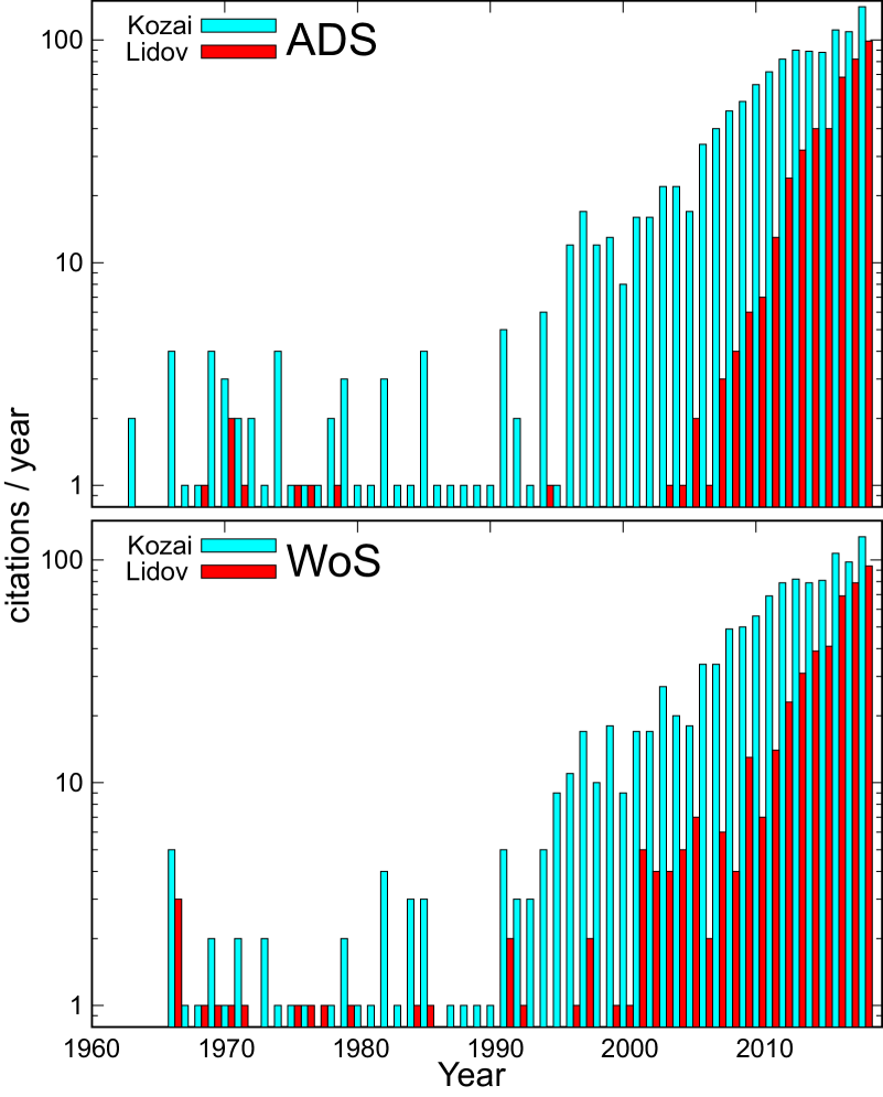
Figure 29: Time series of citation frequencies of Kozai’s publications (cyan bars) and Lidov’s publications (red bars) between 1961 and 2018 based on ADS (upper panel) and WoS (lower panel) as of May 1, 2019. As for the citation data for “Kozai,” we bunched the citation frequencies of two publications: The main paper (Kozai, 1962) and a meeting abstract by the same author with the same title published in the same issue of the same journal (abstracts of papers presented at the 111th Meeting of the American Astronomical Society at Yale University, New Haven, Connecticut, August 26–29, 1962, on p. 579 of The Astronomical Journal, 67, 1962). Similarly, as for the citation data for “Lidov,” we bunched the citation frequencies of closely relevant publications: The original publication (Lidov, 1961), its English translations (Lidov, 1962, 1963a), and the papers with the same subject (Lidov, 1963b, c).

According to the rapid increase of attention to Lidov’s work, more and more people began using the prefix “Lidov–Kozai,” not just “Kozai,” for designating this subject. As far as we have done searches on ADS and WoS, Michtchenko et al. (2006, in their abstract) seems to be the first publication that used the prefix “Lidov–Kozai” (as “the Lidov–Kozai resonance”). On the other hand, the prefix “Kozai–Lidov” showed up first in S̆idlichovský (2005, in their abstract, as “Kozai–Lidov resonance”). Recently, we even find publications that use the prefix “Lidov–Kozai” but cite only Lidov (1961), not Kozai (1962), such as Ulivieri et al. (2013).

6.2.4 Interrelation to Kozai’s work

Here, we would like to mention some interrelation between Lidov’s work and Kozai’s work. These two works have been so far presumed to have been independently carried out. However, this may not be entirely true.

Lidov’s work (including its English translations) on this subject, as well as Kozai’s work, were mainly published between 1961 and 1964. Let us itemize some major relevant events that happened during this period along a timeline:

• Sometime in 1961, Lidov (1961) was published in Iskusstvennyye Sputniki Zemli. Note that the publication of this paper could be earlier or later than the international conference in Moscow that we mention below. We could not identify the exact publication date.

• On November 20–25, 1961, there was a conference on general and applied problems of theoretical astronomy in Moscow. Grebenikov (1962) made a detailed report of this conference. Lidov participated in it and gave a presentation on the subject that we have discussed in this monograph. Kozai was also invited to this conference as a part of the US delegation (at that time Kozai was working at the Smithsonian Astrophysics Observatory, Massachusetts, USA), and gave a talk about the motion of close artificial satellites. Kozai and Lidov met each other at this conference, and had a short conversation (Kozai 2017, personal communication). It was their first and their last direct encounter.

• On May 28–30, 1962, an IUTAM (International Union of Theoretical and Applied Mechanics) symposium on the dynamics of satellites was held in Paris. This time Lidov did not attend the conference, but his presentation was delivered by a delegate (Shevchenko, 2017, his footnote 4 on p. 7). Meanwhile, Kozai participated in the symposium and gave a presentation on the gravitational potential of the Earth derived from satellite motions. Note also that L. I. Sedov who worked on the spacecraft Luna-3’s peculiar motion (see p. 2 of this monograph) was present at this symposium. In Obi et al. (1979) we find a group photo of the symposium participants including both Kozai and Sedov.

• On August 26–29, 1962, Kozai’s work on this subject was (presumably) first unveiled as a paper presented at the 111th Meeting of the American Astronomical Society. See the caption of Fig. 29 for more details.

• On August 29, 1962, Kozai (1962) was received by The Astronomical Journal.

• In October 1962, the first English translation of Lidov (1961) was published in Planetary and Space Science (Lidov, 1962).

• In November 1962, Kozai (1962) was published in The Astronomical Journal.

• In August 1963, the second English translation of Lidov (1961) was published in AIAA Journal Russian Supplement (Lidov, 1963a).

• Sometime in 1963, two proceedings volumes were published. One of them (Subbotin et al., 1963) was the proceedings volume of the 1961 Moscow conference that contains Lidov (1963b) and Kozai (1963b), both of which were written in Russian. The other one (Roy, 1963) was the proceedings volume of the 1962 Paris symposium that contains Lidov (1963c) and Kozai (1963a), both of which were written in English.

• Sometime in 1964, the Moscow 1961 conference proceedings were translated into English and published (Lidov, 1964; Kozai, 1964).

It seems that, at some later point Lidov recognized Kozai’s work when he extended his study on this subject. For example, Lidov and Ziglin (1974) cites Kozai (1962). Also, Lidov uses the Hamiltonian formalism in his later publication such as Lidov and Ziglin (1974, 1976), similar to Kozai. Meanwhile Kozai had recognized Lidov’s work earlier, and cited Lidov’s presentation given at the 1962 Paris symposium in Kozai (1962, p. K591) as “A lunar problem with high inclination was similarly studied by Lidov (1962),” with the corresponding reference of “Lidov, M. L. 1962, Paper presented at the International Symposium on Dynamics of Satellites, Paris” (p. K598). In addition, the AIAA version of the English translation of Lidov’s work seems to be officially “reviewed” by Kozai. A footnote in Lidov (1963a) says:

“Translated from Iskusstvennye Sputniki Zemli (Artificial Earth Satellites) (Academy of Science Press, Moscow, 1961), No. 8, pp. 5–45. Translated by Jean Findlay, Green Bank, West Va. Reviewed by Yoshide Kozai, Smithsonian Astrophysical Observatory, Cambridge, Mass.” (p. 1985)

Therefore, it is possible that the five extra paragraphs found at the leading part of Lidov (1963a) that we mentioned in Section 4.2 (p. 4.2 of this monograph), which the original version (Lidov, 1961) and the other translation (Lidov, 1962) do not contain, may have been added by the reviewer, Kozai. Note that Kozai’s first name is wrongly typed in the above: “Yoshide” should be “Yoshihide”.

Bearing these circumstances in mind, we collectively judge that Lidov’s work and Kozai’s work thus interacted with each other, unlike the common view that they were independently carried out without any interaction. Some people may have been already aware of the personal interrelation between Lidov and Kozai before we did. For example, Tremaine and Yavetz (2014) presents a description of the history of the Lidov–Kozai oscillation study:

“The nonlinear trajectories of the linear instabilities we have described are known as Kozai, Kozai–Lidov, or Lidov–Kozai oscillations. Although Laplace had all of the tools needed to investigate this phenomenon, it was only discovered in the early 1960s by Lidov in the Soviet Union and brought to the West by Kozai.” (at the beginning of their Section IV, in the left column of p. 776)

We are not sure if Tremaine and Yavetz knew that Lidov and Kozai met each other at the conference in Moscow in 1961. But the above description literally claims that Lidov recognized the dynamical phenomenon first, and then Kozai spread it over the western community after that. However recall that, in this monograph, we are not going to judge which should be called the first and which should be the second between Lidov and Kozai. We do not think this kind of discussion has a significant meaning anymore, as we now know that von Zeipel had recognized this dynamical mechanism much earlier than Lidov or Kozai did. We are not yet familiar with what Laplace did along this line of work as Tremaine and Yavetz pointed out, but we will continue to investigate this historical theme.

6.2.5 Choice of terms

At the end of this subsection let us deviate from Lidov’s work, and think more generally about the terms that people use for describing the secular dynamical phenomena that we deal with. In this monograph, we have basically used the term “the Lidov–Kozai oscillation,” because we want to emphasize the oscillating nature of the phenomenon. However, as readers are well aware, different people make different choice of words on this same phenomenon other than oscillation. So it may be interesting to consider how people have collectively called this secular dynamics in the past literature.

To this end, we carried out a simple search on the abstracts of all bibliographic sources registered on ADS (i.e. refereed and non-refereed publications in astronomy and physics) using a series of keywords, “Kozai —” and “Lidov —”. Here, “—” is either of the following words: mechanism, resonance, cycle, oscillation, effect, dynamics, perturbation, or libration. Note that this is not an AND (logical conjunction) search: We just used fixed, consecutive phrases such as “Kozai mechanism”, not “Kozai” AND “mechanism”. Thus we are supposed to count the number of the ADS abstracts that contain the phrase “$\ast$Kozai mechanism$\ast$” where $\ast$ denotes the wildcard match. Naturally, the search result would include “Lidov–Kozai mechanism”. Similarly, a phrase search “Lidov mechanism” on ADS is equivalent to the search of “$\ast$Lidov mechanism$\ast$” which would also find “Kozai–Lidov mechanism”. We applied the same procedure to other words (resonance, cycle, oscillation, $\cdots$). We are aware that this kind of simple search overlooks relevant expressions such as “Lidov–Kozai secular dynamics” or “Kozai–Lidov resonant effect”. However, although it is a crude statistical method, through this search we can find a general tendency as to which term the authors of past literature have preferred for describing this secular dynamics.

Table 6: Result of our abstract search through ADS as of May 1, 2019. Let us explain how the table should be read by taking the line for the word mechanism as an example. On this line, the first number (157) means that we found 157 abstracts containing the expression “$\ast$Kozai mechanism$\ast$”. This includes the abstracts that contain expressions such as “Lidov–Kozai mechanism”. The second number (66) means that we found 66 abstracts containing the expression “$\ast$Lidov mechanism$\ast$”. This includes the abstracts that contain expressions such as “Kozai–Lidov mechanism”. The total number of the abstracts that contain the expression “$\ast$Kozai mechanism$\ast$” or “$\ast$Lidov mechanism$\ast$” is thus $157+66=223$, as indicated in the right-hand column. Note that our search targets were all bibliographic sources in astronomy and physics registered on ADS. These include non-refereed publications such as conference abstracts, proceedings, and the arXiv e-prints. Note also that we carried out the same search using several other words as well (circulation, state, phenomenon, behavior, motion), and ended up with a null result.

word in “—”	Kozai —	Lidov —	total
mechanism	157	66	223
resonance	157	10	167
cycle	103	18	121
oscillation	76	43	119
effect	39	13	52
perturbation	7	6	13
dynamics	9	3	12
libration	7	0	7

We summarized our search result in Table 6. Note that the resulting statistics would be different if we do the same kind of search through the full text of the literature. But as the full text search of all the literature is practically impossible, we just have to presume that the abstracts overall represent the common preference in the academic world.

Among the words tabulated in the leftmost column of Table 6, particularly the most popular ones (mechanism, resonance, cycle, oscillation, and effect), we prefer to use oscillation in this monograph. Mechanism, which is seen most frequently for expressing the subject, generally emphasizes (in our opinion) an internalized dynamical structure rather than the apparent, manifested characteristics it realizes. We think that the accomplishment of Lidov and Kozai should be acknowledged in the first place by their quantitative and accurate recognition of the apparent, overt phenomenon itself (oscillation), followed by the detailed inspection of what causes it (mechanism). Resonance is also common according to the statistics shown in Table 6, but we think this term is not entirely appropriate for denoting this subject. It is because a resonance in general is supposed to work between a frequency that one object (or phenomenon) possesses and another frequency that another object (or phenomenon) possesses. For example, mean motion resonance between Jupiter and an asteroid, spin-orbit resonance between planetary rotation and its revolution, secular resonance between a forced orbital frequency and an intrinsic (proper) orbital frequency, and so forth. But in the considered problem (CR3BP) that practically has only two objects, the perturber’s motion does not have any frequencies after averaging: All of its orbital elements become constant or vanish. If we purposely search any resonance-related argument in the system, it would be the relation $g=\pm\frac{\pi}{2}$ seen in the libration of perturbed body’s argument of pericenter. However, this involves just one variable of just an object. Therefore we would like to avoid using the word resonance here. Effect sounds okay, but we think this word’s meaning can be too broad for the purpose. Cycle sounds as fine as oscillation, and we could bring this word up as our best preference instead. The only concern of ours is that we are not quite sure if we can safely use the term cycle for a non-cyclic phenomenon such as what emerges when the eccentricity of the perturbing body is in effect (see Fig. 4 of this monograph). In the end, the word oscillation sounds relatively better for us and more appropriate than others. This word describes an externally manifested characteristic of the phenomenon. Also, we can probably use oscillation for non-cyclic phenomena, such as seen in Fig. 4, more safely than cycle.

However, there is obviously a large uncertainty and degrees of freedom in the choice of terms here. Although we will continue preferring the term oscillation in this monograph, readers can choose other appropriate words at their discretion as long as the selected word does not introduce unnecessary mix-up or misunderstanding.

6.3 Achievements of von Zeipel’s work

Published more than fifty years before the works of Lidov and Kozai, we can regard von Zeipel’s work as a pioneering manifestation of the application of the Lindstedt series to the theoretical framework of the doubly averaged CR3BP. Standing on the fundamentals of celestial mechanics that had been established by his time, von Zeipel clearly manifested, in the form of the Lindstedt series, the existence of stationary points and periodic trajectories that show up in perturbed body’s motion in the doubly averaged CR3BP.

After making a general and detailed mathematical preparation for how he deals with the Lindstedt series, von Zeipel moves on to considering the actual doubly averaged disturbing function for CR3BP. One of the interesting aspects of his work is that he focuses on the topology of the disturbing potential’s surface. He first searches local extremums of the doubly averaged disturbing function $R$ by calculating the first derivatives of $R$ such as $\frac{\partial R}{\partial\left(e^{2}\right)}$. Then he calculates the second derivatives such as $\frac{\partial^{2}R}{\partial\left(e^{2}\right){}^{2}}$ to confirm whether the discovered local extremum is a local minimum, a local maximum, or a saddle point. As a result, von Zeipel found that the doubly averaged disturbing function for the inner CR3BP $(\alpha<1)$ possesses a pair of local minima along the axis of $g=\pm\frac{\pi}{2}$ when $k^{2}=\left(1-e^{2}\right)\cos^{2}I<\frac{3}{5}$ in the limit of $\alpha\ll 1$ (Section 5.6 of this monograph). Evidently, this result is equivalent to those found by Lidov and Kozai years later. Although handwritten, von Zeipel drew a pair of equi-potential diagrams for two possible modes: One is for the case when perturbed body’s argument of pericenter $g$ circulates from 0 to $2\pi$, and the other is for the case when $g$ librates around $g=\pm\frac{\pi}{2}$ (Fig. 13 of this monograph). In the limit of $\alpha\ll 1$, he gave an explicit function form of perturbed body’s eccentricity at the equilibrium points ($e_{0.2}$ in Eq. (Z81-269)). In von Zeipel’s work, there is no mention on parameters relevant to Lidov’s $c_{2}$.

von Zeipel extended his theory to a more general inner CR3BP where $\alpha$ is not very small. Based on a set of formulas presented in Tisserand’s work, von Zeipel obtained numerical values of $R$ as a function of $\alpha$ and $I_{0}\equiv\cos^{-1}k$ (Fig. 14 of this monograph). This enabled him to estimate numerical values of the smallest inclination $I_{0.2}$ and its dependence on $\alpha$ for the local minima of $R$ to show up along the axis of $g=\pm\frac{\pi}{2}$. His result turned out almost identical to what Kozai later obtained (Fig. 15 of this monograph).

What makes von Zeipel’s work unique and different from Kozai’s or Lidov’s is the fact that he dealt with not only the inner CR3BP but also the outer CR3BP where $\alpha>1$ (Section 5.7 of this monograph). Similar to the way he studied the inner problem, von Zeipel paid attention to the topology of the disturbing potential’s surface, and searched local extremums of the doubly averaged disturbing function $R$ for the outer CR3BP by calculating its first and second derivatives. As a result, he found that in the limit of very small $\alpha^{\prime}$ $\left(=\alpha^{-1}\right)$, $R$ possesses various local extremums when $k^{2}<\frac{1}{5}$: The origin $(e\cos g,e\sin g)=(0,0)$ can be a local maximum, a local minimum, or a saddle point. Also, a pair of local minima along the axis of $g=\pm\frac{\pi}{2}$ can show up. In addition, a pair of saddle points along the axis of $g=0$ or $g=\pi$ can take place. von Zeipel also left a triplet of handwritten equi-potential diagrams for three possible modes (Fig. 17 of this monograph). In the limit of $\alpha^{\prime}\ll 1$, von Zeipel gave explicit function forms of perturbed body’s eccentricity at the equilibrium points ($e^{\prime}_{2.0}$ in Eq. (Z103-340) and $e^{\prime}_{0.2}$ in Eq. (Z104-341)) in the same way as he did for the inner problem.

Similar to his treatment of the inner problem, von Zeipel then extended his theory to a more general outer CR3BP where $\alpha^{\prime}$ is not very small. As a result, he obtained numerical values of $R$ as a function of $\alpha^{\prime}$ and $I_{0}$ (Fig. 18 of this monograph). This enabled him to estimate the numerical values of the smallest inclinations ($I^{\prime}_{2.0}$ and $I^{\prime}_{0.2}$) and their dependence on $\alpha^{\prime}$ for the local extremums of $R$ to show up. His results agree well with our numerical confirmation (Fig. 22 of this monograph), although influence of mean motion resonance was not taken into account in his work.

As we mentioned on p. 5.7 of this monograph, studies of the outer CR3BP lagged behind those of the inner problem until the 1990s, when people came to seriously realize the existence of TNOs and extrasolar planets. After the discoveries of these objects, we find many more serious studies on the outer CR3BP. But in von Zeipel’s era, the only “outer” objects that satisfied the condition $\alpha>1$ were just some comets, while many more “inner” objects (main belt asteroids) were recognized. In this regard, we are impressed by the fact that von Zeipel dealt with the outer problem in an equivalent manner and depth to the inner problem.

von Zeipel applied his theory to the actual asteroids in the solar system. Among the 665 asteroids that were recognized at that time, he chose six of them as candidates that may have a large secular oscillation of eccentricity because they have large inclinations (p. 5.6.3 of this monograph). Although none of the six asteroids turns out to be a $g$-librator (Fig. 16), we found, from a modern viewpoint, that two of the six asteroids that von Zeipel picked ((2) Pallas and (531) Zerlina) belong to the Pallas family. The other four asteroids also have similar orbital elements. Therefore in hindsight, we may want to say that von Zeipel unintentionally approached the theoretical recognition of asteroid families earlier than Kiyotsugu Hirayama (Hirayama, 1918, 1922) who is regarded the first to advocate the concept of asteroid families based on the theory of proper orbital elements. However, we are sure that von Zeipel’s interest was just confined to finding unusual asteroids having a large secular oscillation of eccentricity and inclination, and that finding or recognizing family-like groups of small bodies was not his priority.

von Zeipel also discussed the motion of two actual comets in the solar system: 1P/Halley (Section Z21. See our Section 5.8.1 of this monograph), and 2P/Encke (Section Z29). The discussion on the motion of 1P/Halley is particularly quantitative and detailed. von Zeipel made an accurate calculation of the location of the equilibrium points of the doubly averaged disturbing function for 1P/Halley (Figs. 26 and 27 of this monograph), although his treatment was limited to the framework of a doubly averaged CR3BP where Jupiter on a circular orbit serves as the only perturber.

von Zeipel further extended his theory for investigating more subjects, and came to further quantitative conclusions. One of them is the calculation of the doubly averaged disturbing function of CR3BP when the orbits of the perturbed and perturbing bodies act like rings in a chain. As we mentioned in Section 5.8 of this monograph, it seems that this subject had not been seriously investigated until Gronchi and Milani (1998, 1999) worked on it. Another extension is a treatment of the motion of the perturbed body using a different set of canonical variables when its eccentricity is close to the maximum, $k^{\prime}$ (Section 5.9.1 of this monograph). Here, von Zeipel stated that a perturbed body’s orbit with a large eccentricity and small inclination outside the perturber’s orbit can stably exist. Again in a modern viewpoint, we might want to regard this statement as his unintentional prediction of the existence of the scattered TNOs (with a small inclination). Yet another example of his theoretical extensions are the outline of the method to deal with systems with multiple perturbing bodies (Section 5.9.2 of this monograph). To date, this approximation has been refined and made more sophisticated, and is extensively used in modern solar system dynamics as we mentioned in Section 5.9.2.

6.4 Earlier studies by von Zeipel

Earlier in this monograph (p. 5.4), we wrote that von Zeipel’s work in 1910, particularly the subject in its Chapter II, can be regarded as a prototype study that was later developed into a more sophisticated canonical perturbation theory. From a broader historical perspective, we understand that von Zeipel (1910) occupies an important midpoint in the major flow of celestial mechanics that showed remarkable development from the late nineteenth century to the early twentieth century. The flow was established by the giants of that era (examples of major publications: Tisserand, 1889, 1891a, 1894, 1896; Picard, 1891, 1893, 1896; Poincaré, 1892, 1893, 1899, 1905, 1907, 1909, 1910; Birkhoff, 1913, 1915, 1922, 1926). And, von Zeipel himself undoubtedly belongs to the giants due to his own outstanding achievements.

Although we wrote about von Zeipel’s essential contribution to the historical flow of celestial mechanics, we are sure that very few people have been aware of his work published in 1910. And, we are surer that even fewer people know that there are two more studies by von Zeipel published earlier than 1910: von Zeipel (1898, 1901). We regard these publications as being forerunners of later, more complete products (e.g. von Zeipel, 1905, 1910, 1915, 1916a, 1916b, 1917a, 1917b). In the present subsection, we make a brief summary of von Zeipel’s achievement in the two early papers. He may have published more work along these lines prior to 1898, but so far we have not found any others than these two.

6.4.1 von Zeipel (1898)

von Zeipel dealt with the full three-body problem in both his 1898 and 1901 papers, and regarded the restricted problem as an extreme case. The first paper (von Zeipel, 1898) is entitled “Sur la forme géńerale des éléments elliptiques dans le problème des trois corps,” written in French and published in Bihang till Kongl Svenska Vetenskaps–Akademiens Handlingar. This paper begins with a series of equations that defines the system that he considers, without any descriptions on the purpose or background of his intentions. Literally citing the first part of the paper, we see that von Zeipel deals with the general three-body system described in the Jacobi coordinates:

“It is assumed that the masses $m_{1}$ and $m_{2}$ are small with respect to the mass $m_{0}$ and that $m_{1}$ and $m_{2}$ are of the same order of magnitude. The motion of $m_{1}$ is referred to a system of coordinates whose origin is situated in $m_{0}$ and whose axes retain the same directions. The coordinates of $m_{1}$ in this system are $x_{1}$, $y_{1}$, $z_{1}$. The center of gravity of the masses $m_{0}$ and $m_{1}$ is the origin of another system of coordinates, the axes of which are parallel to the axes of the first. The coordinates of $m_{2}$ in the latter system are $x_{2}$, $y_{2}$, $z_{2}$. If the masses $m_{1}$, $m_{2}$, $m_{3}$ attract according to Newton’s law, the equations of motion are [$\ldots$],” (p. 3)

After this, a description of the standard canonical equations of motion using the three-body Hamiltonian follows.

von Zeipel’s intention in his 1898 paper is to show that, as long as the orbits in a three-body system are roughly circular (i.e. both the bodies have small eccentricity), it is possible to construct approximate solutions for their orbital variation in the form of trigonometric series without generating terms that secularly increase. Although von Zeipel does not use the word Lindstedt at all in this paper, it is obvious that this series is nothing but the Lindstedt series. Also, from his assumption that the eccentricities of the bodies are small, we presume that he tried to construct the Lindstedt series around the origin $(0,0)$ on the $(e\cos g,e\sin g)$ plane.

In this paper von Zeipel utilizes the result given in Tisserand (1889) for obtaining the function form of the averaged Hamiltonian (referred to as $[F_{1}]$) when the eccentricities of both the bodies are small (Eq. (5) on his p. 12). Going through similar mathematical procedures that we have seen in Section 5.4 of this monograph, von Zeipel searches conditions for the series to exist—conditions that the orbital elements are expressed in trigonometric series that do not contain secularly increasing terms.

von Zeipel eventually found that the series he seeks exists if the pair of solutions of a quadratic equation become unequal and negative. The quadratic (actually, a quartic) equation that he mentions appears on his p. 23 as follows:

$$\alpha^{(1)4}+\left\{a_{11}^{(1)}c_{11}^{(1)}+2a_{12}^{(1)}c_{21}^{(1)}+a_{22}^{(1)}c_{22}^{(1)}\right\}\alpha^{(1)2}$$

$$\quad\quad\quad+\left|\begin{array}[]{cc}a_{11}^{(1)}&a_{12}^{(1)}\\ a_{21}^{(1)}&a_{22}^{(1)}\\ \end{array}\right|\left|\begin{array}[]{cc}c_{11}^{(1)}&c_{12}^{(1)}\\ c_{21}^{(1)}&c_{22}^{(1)}\\ \end{array}\right|=0. \alpha$$ ()

An equivalent equation shows up again on his p. 47 as:

$$x^{4} +\left\{a_{11}c_{11}+2a_{12}c_{12}+a_{22}c_{22}\right\}x^{2}$$

$$\quad\quad+\left|\begin{array}[]{cc}a_{11}&a_{12}\\ a_{21}&a_{22}\\ \end{array}\right|\left|\begin{array}[]{cc}c_{11}&c_{12}\\ c_{21}&c_{22}\\ \end{array}\right|=0, \alpha$$ ()

with the coefficients defined as:

$$a_{ik}=\frac{\partial^{2}[F_{1}]}{\partial\xi_{i}\partial\xi_{k}},\>\>c_{ik}=\frac{\partial^{2}[F_{1}]}{\partial\eta_{i}\partial\eta_{k}},\>\>(i,k=1,2)$$ (400)

together with other variables defined as:

$$\xi_{k} =\>\>\>\sqrt{2\left(\Lambda_{k}-H_{k}\right)}\cos g_{k},$$ (401)

$$\eta_{k} =-\sqrt{2\left(\Lambda_{k}-H_{k}\right)}\sin g_{k},$$ (402)

$$\Lambda_{k} =\beta_{k}L_{k},\>\>H_{k}=\beta_{k}G_{k},$$ (403)

where $L_{k},G_{k},g_{k}$ $(k=1,2)$ are Delaunay elements with

$$\beta_{1} =\frac{\mu_{0}}{\mu_{1}}, \;\;\;\;\beta_{2} =\frac{\mu_{1}}{\mu_{2}}\frac{m_{2}}{m_{1}},$$ (404)

$$\mu_{1} =m_{0}+m_{1}, \;\;\;\;\mu_{2} =m_{0}+m_{1}+m_{2},$$ (405)

and $\mu_{0}=m_{0}$. von Zeipel only showed approximate forms of the coefficients $a_{11},c_{11},a_{22},\cdots$ on his p. 50. Exhibiting specific function forms of these coefficients is a major subject of his next paper (von Zeipel, 1901). Here he just yields his final result—a pair of solutions of Eq. $(\alpha)$ as:

$$x_{1}^{2} =-A^{2}\left\{\left(5\cos^{2}J_{0}-1+2\frac{m}{m^{\prime}}\sqrt{\alpha}\cos J_{0}\right)^{2}\right.$$

$$\quad\quad\quad\quad\quad\quad\quad\quad\quad\quad\left.-25\sin^{4}J_{0}\biggr{\}}\right.+\cdots,$$ (406)

$$x_{2}^{2} =-A^{2}\left\{\left(5\cos^{2}J_{0}-1\right)\frac{m}{m^{\prime}}\sqrt{\alpha}+2\cos J_{0}\right\}^{2}+\cdots,$$ (407)

where $J_{0}$ is the initial mutual inclination of the orbits of the two bodies, $A$ is a positive coefficient that is a function of $\alpha^{2}$ where $\alpha$ is the ratio of semimajor axis, $\frac{a}{a^{\prime}}$ or $\frac{a_{1}}{a_{2}}$. We presume that $m$ and $m^{\prime}$ are the masses of the inner and outer bodies, respectively, although von Zeipel did not leave any specific definitions of them in this paper.

Using $x_{1}$ in Eq. (406) and $x_{2}$ in Eq. (407), the condition for the Lindstedt series to exist that von Zeipel mentioned (“the pair of solutions of a quadratic equation become unequal and negative”) is expressed as:

$$x_{1}^{2}<0,\quad x_{2}^{2}<0,\quad x_{1}^{2}\neq x_{2}^{2}.$$ (408)

Then, he makes a conclusion when $\alpha$ is very small as:

“We can conclude that

$$x_{1}^{2}<0 {\cos^{2}J_{0}>\frac{6}{10}}$$    if

$$x_{2}^{2}<0 J_{0}$$    for all the values of

$$x_{1}^{2}\neq x_{2}^{2} {\cos^{2}J_{0}\neq\frac{2}{3}}$$    when

We have

$$\cos^{2}J_{0}=\frac{6}{10}$$

for

$$|J_{0}|=39^{\circ}14^{\prime}\cdots$$

When

$$|J_{0}|>39^{\circ}14^{\prime}\cdots$$

and [when] $\alpha$ is a small quantity, the series of the previous section are in default.” (p. 50)

von Zeipel thus claims that the initial mutual inclination $J_{0}$ cannot exceed $\cos^{-1}\sqrt{\frac{6}{10}}\sim 39^{\circ}14^{\prime}$ for the Lindstedt series to exist. Note that for von Zeipel at that time, the non-existence of the Lindstedt series literally meant the dynamical instability of the entire three-body system.

At the end of his 1898 paper, von Zeipel leaves a paragraph that closes the paper as follows:

“The same thing has been shown before in other ways. Tisserand has generalized the method of Delaunay for the Moon by making a series of transformations, each of which eliminates a part of the disturbing function. In these methods of demonstration, Mr. Poincaré has always used the partial differential equation of Hamilton–Jacobi.” (p. 51)

We are not completely sure what von Zeipel meant by “the same thing” (“la même chose”) here, but we presume that he describes the historic use of canonical transformation in perturbation theories ever since Delaunay. This is particularly true when we mention the elimination of fast-oscillating variables from the disturbing function by averaging.

The critical value of the initial mutual inclination that von Zeipel found in this paper, $J_{0}=\cos^{-1}\sqrt{\frac{6}{10}}$, is evidently equivalent to what Kozai and Lidov found in the doubly averaged inner CR3BP. We have not confirmed whether or not von Zeipel’s third condition, $\cos^{2}J_{0}=\frac{2}{3}$ (that would realize $x_{1}^{2}=x_{2}^{2}$), really causes a problem in this study. But we can at least say that von Zeipel was already aware of the critical value of $\cos^{-1}\sqrt{\frac{6}{10}}\sim 39^{\circ}14^{\prime}$ at the end of the nineteenth century—more than sixty years before the works of Lidov and Kozai came out.

Although von Zeipel dealt with the non-restricted three-body problem with point masses $m_{0}$, $m_{1}$, $m_{2}$ in his 1898 paper, it seems that he did not give deep consideration on the mass ratio such as $\frac{m_{1}}{m_{2}}$. His solutions $x_{1}^{2}$ in Eq. (406) and $x_{2}^{2}$ in Eq. (407) contain terms with the mass ratio $\frac{m}{m^{\prime}}$ as a coefficient. But these terms are ignored when he calculates $J_{0}$ by taking the limit of $\alpha=\frac{a}{a^{\prime}}\to 0$.

6.4.2 von Zeipel (1901)

The next paper (von Zeipel, 1901) is entitled “Recherches sur l’existence des séries de M. Lindstedt,” written in French, and again published in Bihang till Kongl Svenska Vetenskaps–Akademiens Handlingar. It seems that now von Zeipel pays particular attention to the influence of the ratio of the semimajor axes of the two bodies $\left(\alpha=\frac{a}{a^{\prime}}\right)$ on the critical inclination values, when $\alpha$ is not so small. The example used in this study is the Sun–Jupiter–Saturn system where $\alpha\sim 0.5431$.

For better facilitating an understanding of what von Zeipel did in his 1901 publication, let us take a look at a short introductory article, Callandreau (1902), which briefly summarizes what is done in von Zeipel (1901). Let us cite the article in its entirety, since it is very short. Note that Callandreau (1902) was originally written in French, and the following English translation is ours:

“Mr. v. Zeipel thus states the conclusions of his work: If the inclination of the orbit of an asteroid exceeds a certain limit (about $30^{\circ}$, slightly variable with the ratio of the axes), the series of Mr. Lindstedt does not exist. We cannot avoid the secular terms, and the orbit is likely unstable $\ldots$ . Perhaps this is the cause of this surprising fact that, among about 500 small planets, there is only one, Pallas, whose inclination exceeds $30^{\circ}$. It was first necessary to make the study of the series possible, no matter how great the mutual inclination of the orbits [is]; Mr. v. Zeipel took advantage of the work of Jacobi and Tisserand.”

As is seen in its title, von Zeipel frequently uses the term “Lindstedt series” in his 1901 paper. This paper begins with the conclusion of his previous work (1898) as follows. Note that the partial use of the italic characters in the following is by the original author (von Zeipel):

“By means of Mr. Lindstedt’s series, one can, as we know, give the coordinates of the three bodies a form, where time never leaves the signs [of] sin and cos.

In an earlier Mémoire (On the general form of elliptical elements in the problem of three bodies. Bihang Till K. Svenska Vetenskapsakademiens handlingar. Band 24. Afd I. N:o 8) I gave a new exhibition of the series in question by a little generalizing the known theory of Mr. Poincaré for the periodic and asymptotic solutions in the problems of the dynamics.

By eliminating the nodes, as did Jacobi, it was possible to study the series, no matter how great the mutual inclination of the orbits is. So I found (loc. cit.) as necessary and sufficient conditions for the existence of the series of Lindstedt:

1:0 that the orbits are roughly circular.

2:0 that the roots of the equation of the fourth degree

$$\sigma^{4} -\left(a_{1,1}c_{1,1}+2a_{1,2}c_{1,2}+a_{2,2}c_{2,2}\right)\sigma^{2}$$ (Zb1-408)

$$\quad\quad+\left|\begin{array}[]{cc}a_{1,1}&a_{1,2}\\ a_{2,1}&a_{2,2}\\ \end{array}\right|\left|\begin{array}[]{cc}c_{1,1}&c_{1,2}\\ c_{2,1}&c_{2,2}\\ \end{array}\right|=0$$

where

$$a_{ik} =\left.\frac{\partial^{2}\left[\frac{fm_{2}}{\Delta}\right]}{\partial\xi_{i}\partial\xi_{k}}\right|_{\xi_{r}=\eta_{r}=0},$$ (Zb2-409)

$$c_{ik} =\left.\frac{\partial^{2}\left[\frac{fm_{2}}{\Delta}\right]}{\partial\eta_{i}\partial\eta_{k}}\right|_{\xi_{r}=\eta_{r}=0},$$

$$(i,k=1,2)$$

are real and unequal.” (p. 3)

Note that in the above, we renamed the equation numbers in the original publication from (1) to (Zb1-408), and from (2) to (Zb2-409), for avoiding potential confusions. Note also that the small subscript $r$ placed together with the partial derivatives in the right-hand side of Eq. (Zb2-409) as $\xi_{r}=\eta_{r}=0$ means, although von Zeipel (1901) did not explicitly explain, that we must substitute $\xi_{r}=\eta_{r}=0$ (where $r=1$ and $2$) after completing the partial differentiation (see p. 22 and p. 47 of von Zeipel, 1898).

Readers might find that Eq. (Zb1-408) is close to Eq. $(\alpha)$ in von Zeipel (1898). But there are differences:

• The variable $x$ in Eq. $(\alpha)$ has been replaced for the variable $\sigma$ in Eq. (Zb1-408).

• The subscripts of the coefficients in Eq. (Zb1-408) have a comma such as $a_{1,1}$ instead of $a_{11}$ in Eq. $(\alpha)$.

• The sign of the second term in the left-hand side is positive in Eq. $(\alpha)$, while it is negative in Eq. (Zb1-408).

Among the above-mentioned differences, the third one is the most significant. It changes the condition for the existence of the Lindstedt series that expresses the periodic solutions which von Zeipel seeks. More specifically saying,

• von Zeipel (1898, p. 23) depicts the condition as, right after Eq. $(\alpha)$, “The two values of $\alpha^{(1)2}$ are unequal and $<0$”. This means that all solutions $\alpha^{(1)}$ (or $x$ on p. 47) would need to be imaginary.

• von Zeipel (1901, p. 3) depicts the same condition as “the roots of the equation of the fourth degree (Eq. (Zb1-408)) are real and unequal.” Here, the roots designate $\sigma$ in Eq. (Zb1-408).

Although we can show that there is no practical contradiction between the above two, we have no idea why von Zeipel made this change between the two publications.

He then moves on to stating the objective of the entire paper. von Zeipel wrote as follows:

“In the case where the ratio $\alpha$ of the two major axes is very small, the discussion of the equation (Zb1-408) was very simple. We found in this case (loc. cit. p. 50), as the upper limit of the inclination, the value $39^{\circ}.14\ldots$

In this Mémoire I want to give the analytic form of the coefficients $a_{i,k}$ and $c_{i,k}$ in detail. I also want to apply the formulas in a special case by choosing, for $\alpha$, the ratio of the major axes of the orbits of Jupiter and Saturn. The calculation shows that the second condition is no longer fulfilled when the inclination $J_{0}$ exceeds a certain limit, depending on the two ratios $\frac{m_{1}}{m_{2}}$ and $\frac{a_{1}}{a_{2}}$.

We will see, that the limit in question is quite low.” (p. 4)

When he expands the direct part of the disturbing function $\left(\frac{1}{\Delta}\right)$ in this publication, von Zeipel again assumes that the eccentricity of both the two bodies are small. We find his assumption in the following description in his §1:

“To find the form of the coefficients $a_{i,j}$ and $c_{i,k}$ as functions of $m_{1},m_{2}$ and $J_{0}$, we want to develop the function $\frac{1}{\Delta}$ in the increasing powers of eccentricities $e_{1}$ and $e_{2}$. In this development it suffices to write only of the terms of the second degree, as in formulas (Zb2-409) one must place $\xi_{r}=\eta_{r}=0$, i.e. $e_{1}=e_{2}=0$ after differentiation.” (p. 5)

As von Zeipel states above, in his 1901 paper he first aims at expressing the coefficients $a_{i,k}$ and $c_{i,k}$ in Eq. (Zb1-408) using orbital elements. After that, he calculates their numerical values by substituting the actual orbital elements of objects such as Jupiter or Saturn. von Zeipel’s eventual purpose in this paper is to know the dependence of the critical value of the initial mutual inclination $J_{0}$ on the semimajor axis ratio, $\alpha$. In von Zeipel’s theory, as developed at this point, construction of the Lindstedt series would be impossible when $J_{0}$ exceeds the critical value.

The remaining part of his 1901 paper is full of detailed mathematical expositions where von Zeipel expands the disturbing function in a way that is already familiar to us. In the procedure, he employs the same technique that was later used in his 1910 paper—use of the Laplace-like coefficients $b^{i,j}$, $c^{i,j}$, $e^{i,j}$. We already browsed through how he achieved it in Section 5.6.3 of this monograph.

Table 7: A reproduction of an unnumbered table in von Zeipel (1901, p. 22). Note that this table is presented as an equation numbered (32) in von Zeipel’s original paper, not as a table. Note also that von Zeipel’s definition yields the relations $a_{1,2}=a_{2,1}$ and $c_{1,2}=c_{2,1}$. This is based on the symmetry of second derivatives (see Eq. (Zb2-409)).

	$J_{0}=0$	$J_{0}=30^{\circ}$	$J_{0}=45^{\circ}$
$a_{1,1}$	$+32^{\prime\prime}.96$	$+21^{\prime\prime}.70$	$+15^{\prime\prime}.64$
$c_{1,1}$	$+32^{\prime\prime}.96$	$+11^{\prime\prime}.27$	$+1^{\prime\prime}.78$
$a_{2,2}$	$+43^{\prime\prime}.80$	$+19^{\prime\prime}.83$	$+8^{\prime\prime}.39$
$c_{2,2}$	$+43^{\prime\prime}.80$	$+17^{\prime\prime}.16$	$+6^{\prime\prime}.94$
$a_{1,2}$	$-7^{\prime\prime}.58$	$-3^{\prime\prime}.32$	$-1^{\prime\prime}.29$
$c_{1,2}$	$-7^{\prime\prime}.58$	$+1^{\prime\prime}.91$	$+3^{\prime\prime}.64$

After going through a large amount of algebra, von Zeipel reached a set of numerical values of the coefficients on his p. 22. We reproduced these as our Table 7. Using the coefficients, von Zeipel finally attains the solution $\sigma$ of the quadratic equation (Zb1-408) for three values of initial mutual inclination ($J_{0}=0,30^{\circ},45^{\circ}$) under the actual mean motions $(n_{1},n_{2})$ and masses $(m_{1},m_{2})$ of Jupiter and Saturn. Let us rewrite his results that are summarized as an equation (on his p. 22) in a slightly different format:

$$J_{0}=0: \;\;\sigma =\pm 47^{\prime\prime}.68, \;\;\pm 29^{\prime\prime}.07$$ (Zb33-414)

$$J_{0}=30^{\circ}: \;\;\sigma =\pm 18^{\prime\prime}.26, \;\;\pm 15^{\prime\prime}.43$$

$$J_{0}=45^{\circ}: \;\;\sigma =\pm 1^{\prime\prime}.19\sqrt{-1}, \;\;\pm 8^{\prime\prime}.84$$

where $\sqrt{-1}$ denotes the imaginary unit.

From Eq. (Zb33-414) we know that the existence of the Lindstedt series is assured when $J_{0}=0$ and $30^{\circ}$ because all four $\sigma$ are real and unequal. However, this is not the case when $J_{0}=45^{\circ}$ because two of the four $\sigma$ are imaginary $(\sigma=\pm 1^{\prime\prime}.19\sqrt{-1})$. von Zeipel depicts this outcome as follows. Note that the partial use of italic characters in the following is by the original author (von Zeipel):

“By thus increasing the mutual inclination of the orbits of Jupiter and Saturn, the series of Mr. Lindstedt still exist, while $J_{0}$ reaches the value $30^{\circ}$. But $J_{0}$ exceeding a limit slightly less than $45^{\circ}$, the series in question cease to exist. Then it is no longer possible to avoid the secular terms, and the orbits are probably unstable.” (p. 23)

von Zeipel then moves on to a special case when one of the planetary masses is zero—the restricted three-body problem. Citing his description about it:

“If the outer planet is Jupiter, the inner planet has the mean diurnal motion $n_{1}=742^{\prime\prime},2$ (because of the value used for $\alpha$ and the diurnal motion $n_{1}=299^{\prime\prime},1$ of Jupiter). If, moreover, the mass $m_{1}$ of this planet is $=0$, so that it is an asteroid, the roots of equation (Zb1-408) are

$$\sigma\begin{cases}\pm m_{2}n_{1}\sqrt{a_{1,1}^{(2)}c_{1,1}^{(2)}}\\ \pm m_{2}n_{1}\sqrt{a_{2,2}^{(2)}c_{2,2}^{(2)}}\\ \quad\quad=\pm m_{2}n_{1}\frac{\alpha^{2}}{2}\left(c^{1,0}-c^{0,1}\right)\end{cases}$$

The two first roots become imaginary when $J_{0}$ exceeds the limit $31^{\circ}.1\ \ldots$, because, then, $c^{(2)}_{1.1}$ going through zero becomes negative.” (p. 23)

Here, $m_{2}$ is the mass of the perturbing body, and $n_{1}$ is the mean motion of the perturbed body. $a_{1,1}^{(2)}$, $a_{2,2}^{(2)}$, $c_{1,1}^{(2)}$, $c_{2,2}^{(2)}$ are equivalent to $a_{1,1}$, $a_{2,2}$, $c_{1,1}$, $c_{2,2}$ respectively, when $m_{1}=0$ by von Zeipel’s definitions (Eq. (13) on his p. 14, although we do not reproduce them here). $c^{1,0}$ and $c^{0,1}$ are respectively equivalent to the numerical coefficients $c^{1.0}$ and $c^{0.1}$ that we studied before (Section 5.6.3 of this monograph).

von Zeipel’s above conclusion on the critical value of $J_{0}$ in the restricted case $(J_{0}\sim 31^{\circ}.1)$ must be consistent with what he obtained in his 1910 paper. The ratio of mean motions between the inner and the outer bodies in the above example is $\frac{742.2}{299.1}$, which yields the ratio of the semimajor axes $\alpha=\frac{a}{a^{\prime}}=0.545587$. Remember that we have made a plot of the quantity equivalent to $J_{0}$ (which we have designated as $I_{0.2}$ or $i_{0}$ in this monograph) as Fig. 15. There, we saw that $I_{0.2}$ takes a value just above $30^{\circ}$ when $\alpha\sim 0.55$. This is fairly well consistent with von Zeipel’s statement, $J_{0}\sim 31^{\circ}.1$. Recalling that the method that he employed for this purpose was common between his 1901 and 1910 papers, the agreement is no surprise. The surprise is the fact that the dependence of the limiting inclination value ($J_{0}$ or $I_{0.2}$) on the ratio of the semimajor axes $\alpha$ was already discussed, and its precise numerical estimate was accomplished in 1901, the first year of the twentieth century.

The largest difference between the conclusions of von Zeipel’s 1901 paper and 1910 paper is that, by the 1910 work he had made substantial progress in his theory, and showed that a perturbed body’s periodic orbit can stably exist around a disturbing potential’s local minima or maxima even when the initial mutual inclination is larger than the critical value. In his 1910 paper, he proved that we can construct the Lindstedt series providing the doubly averaged disturbing function possesses local minima or maxima. This is what we demonstrated in Section 5 of this monograph. Let us remark that, after his 1901 paper, von Zeipel completed his PhD thesis entitled “Recherches sur les solutions périodiques de la troisièm sorte dans le problème des trois corps,” at Uppsala University (von Zeipel, 1904). Then he moved to the Paris Observatory and stayed there for about two years (from June 1904 through September 1906) to study celestial mechanics more deeply under the supervision of Henri Poincaré and Paul Painlevé before his 1910 paper came out (McGehee, 1986; Barrow-Green, 1996).

At the end of his 1901 paper, von Zeipel made the following concluding statement. Note again that the partial use of the italic characters is due to him:

“We have previously found (see my Mémoire On the general form etc. p. 50) that for a planet very close to the Sun, the corresponding limit was $39^{\circ}2\ldots$ .

We can therefore state the following theorem:

If the inclination of the orbit of an asteroid exceeds a certain limit (about $30^{\circ}$, slightly variable with $\alpha$), the series of Mr. Lindstedt (the absolute orbit of Gyldén) does not exist. Secular terms cannot be avoided, and the orbit is likely unstable.

Although the series of Mr. Lindstedt are only semi-convergent, it is possible to see in this theorem, the cause of this surprising fact, that among about 500 small planets there is only one (Pallas) whose inclination exceeds $30^{\circ}$.” (p. 23)

The above conjecture on the inclination distribution of small planets (“petite planètes” in the original expression. Most of them were the main belt asteroids at his time) is probably associated with a description in his 1910 paper (Section Z19 in Chapter IV. See p. 5.6.3 of this monograph). Nowadays, more and more asteroids are being recognized with inclination larger than $30^{\circ}$, although they do not constitute the majority of the population (e.g. Ivezić et al., 2001; Warner et al., 2009; Novaković et al., 2011). Also, it is now widely believed that the orbital distribution of asteroids is sculptured not only by the secular three-body dynamics but also by complicated processes including the radial migration of major planets (e.g. Morbidelli et al., 2010; Walsh et al., 2011; Lykawka and Ito, 2013, 2017, 2019; Roig and Nesvorný, 2015). Therefore from a modern viewpoint, von Zeipel’s above statement may not be totally accurate.

However, we should also note that von Zeipel’s statement is true about some part of the actual solar system structure. One of the typical examples is the irregular satellites of the jovian giant planets (e.g. Jewitt, 2005; Sheppard, 2006; Bottke et al., 2010). In particular, Nesvorný et al. (2003) carried out numerical simulations and an analytic estimate for explaining the orbital inclination distribution of the irregular satellites of the jovian giant planets that are rather concentrated near ecliptic. As a result, Nesvorný et al. found that the satellite orbits that are highly inclined with respect to ecliptic can become unstable due to “Kozai resonance.” As we learned, this radially stretches the orbits of the satellites until they get out of planetary Hill spheres, collide with other massive satellites, or hit the mother planet. We consider this as a typical manifestation of von Zeipel’s conjecture.

Another example is the near-Earth asteroids with a small perihelion distance. These objects are sometimes called near-Sun asteroids (e.g. Emel’yanenko, 2017) or near-Sun comets (e.g. Jones et al., 2018). Using the latest, self-consistent stationary dynamical model of the near-Earth asteroid distribution, Granvik et al. (2016, 2018) showed that the actually observed near-Earth asteroids with a small perihelion distance (such as $q=a(1-e)<0.2$ au) are much fewer than that predicted by conventional dynamical models. This result can be interpreted as a consequence of catastrophic disruption of the asteroids by the thermal effect when they approach the Sun very closely. Also, many of these asteroids are known to be in the “Lidov–Kozai state” that enhances their eccentricity and inclination (e.g. Ohtsuka et al., 2006, 2007, 2008, 2009; Urakawa et al., 2014), which is possibly causing their thermal metamorphism and disintegration in the end (e.g. German, 2010; Delbo et al., 2014; Ito et al., 2018). It is also worth a mention that the distribution of the argument of perihelion of the Apollo near-Earth asteroids (Earth-crossing objects with a semimajor axis $a>1.0$ au and perihelion distance $q<1.017$ au) shows a non-uniform distribution, which can be attributed to the “Kozai effect” arising from Jovian perturbation (JeongAhn and Malhotra, 2014). An orbital alignment pattern that was recently recognized among the main belt comet population (Kim et al., 2018) may have relevance to this. Therefore, we would say that von Zeipel’s conjecture that the secular three-body dynamical mechanism he found has reduced the number of “small planets” with a large inclination is partially true.

6.5 Consideration on historical examples

Going through von Zeipel’s series of works, we became strongly impressed by how accurate his theories and calculations are on the motion of perturbed bodies in the doubly averaged CR3BP whether it is the inner problem or the outer one. We should recall the fact that electronic computers did not exist at all in his era. Therefore his “numerical” calculations must have been done manually. Nevertheless his numerical results show a beautiful agreement with much later studies that exploited high-speed digital computers, as we have confirmed (see Figs. 15, 22, 26, and 27).

In addition, we should recall that during von Zeipel’s era, observational evidence on the small solar system bodies was still very limited. In Berliner Astronomisches Jahrbuch für 1911 that von Zeipel cited, only about 650 main belt asteroids, a handful of Jupiter Trojans, and just one near-Earth asteroid ((433) Eros) were listed. The number of comets that were recognized at that time was about 400 (this number comes from our own estimate using the list of comets and dates of their first observations registered in the JPL Small-Body Database Search Engine). The asteroid (1373) Cincinnati that Kozai brought up as an example of the $g$-librators was not discovered until 1935. There was no artificial satellite like Luna-3 whose dynamical behavior became a motivation of Lidov’s work. Discoveries of Centaurs did not come until the 1970s. It is needless to mention TNOs or extrasolar planets that were not discovered until the 1990s.

Recognizing the limitations of scientific knowledge and tools at his time, we are impressed by how strongly motivated von Zeipel was on advancing celestial mechanics toward the foundation of theories that can deal with the orbital motion of the small solar system bodies in a comprehensive way. We surmise that his eventual motivation was oriented toward an understanding of the origin and evolution of the entire solar system. In vindication, let us pick some of his occasional statements on the dynamical evolution of the solar system bodies in his publications. One example is von Zeipel’s (1901, p. 23) statement on the fact that most asteroids (recognized at his time) have a smaller inclination than $30^{\circ}$ together with a conjecture on this. We mentioned it in Section 6.4.2 of this monograph. As another example, let us take up a paragraph placed at the end of Section Z19 of von Zeipel (1910) that describes possible dynamical processes that he thought took place in the early solar system. This paragraph appears after he presented the calculation results of $I_{0}$ and $I_{0.2}$ for several actual asteroids (p. 5.6.3 of this monograph). Citing the entire paragraph:

“We shall here make an important remark from the point of view of the evolution of the planetary system. Let us suppose that there is resistance in space against the motion. It is well known that it will have the effect of making the eccentricities (and the major axes) smaller and smaller, finally reducing them to zero. But then, by virtue of what preceded, the combined effect of the resistance and of secular perturbations of an outer planet will also inevitably diminish the inclinations, and lower them more or less below the limit $I_{0.2}$. Then, if the resistance is greater against the retrograde motion, the particles that turn [around the Sun] in the reverse direction will be drawn earlier towards the Sun than the others. There will thus come a time when the originally chaotic nebula will have, at the interior of a disturbing and dominant mass (Jupiter), the present aspect of our solar system.” (p. Z392)

We can presume that, through the above paragraph, von Zeipel intended to give an explanation on the current status of the solar system where most of the bodies are on prograde and only slightly or moderately inclined orbits. At present, it is known that the solar system formation was a combination of many physical processes that interacted with each other. The couple of secular orbital change and nebula gas dynamics that von Zeipel mentioned in the above must have been at work too, at least partially, on forming some part of the current solar system status. Moreover, it is becoming better known that the secular orbital oscillation that von Zeipel discussed efficiently works on shaping some sort of extrasolar planetary systems in combination with tidal interactions with central star and scatterings between planets (e.g. Wu, 2003; Fabrycky and Tremaine, 2007; Narita et al., 2009; Hébrard et al., 2011). Thus, one may want to say that von Zeipel’s statements on the solar system evolution based on his own theory hold true to a certain extent even today.

At this point, we would like to express the following opinion. Considering the fact that von Zeipel far preceded Lidov and Kozai, we believe it is perfectly reasonable to call the theoretical framework and its outcome that we have discussed, “the von Zeipel–Lidov–Kozai oscillation,” instead of using the term Lidov–Kozai or Kozai–Lidov. To reinforce our opinion, let us pick up some historical examples for reference: Rodrigues’ formula, Laplace–Runge–Lenz vector, Yarkovsky effect, and Kuiper belt.

Rodrigues’ formula

Rodrigues’ formula is a famous formula that generates the Legendre polynomial $P_{n}(x)$. It is one of the typical examples whose name changed as its earlier pioneer got recognized later. The formula is expressed as follows (e.g. Stegun, 1965, p. 334):

$$P_{n}(x)=\frac{1}{2^{n}n!}\frac{d^{n}}{dx{}^{n}}\left(x^{2}-1\right)^{n}.$$ (416)

According to Askey (2005, pp. 105–106), this formula first appeared in Rodrigues (1816) as Olinde Rodrigues’ doctoral dissertation. However, Ivory (1824) and Jacobi (1827) made equivalent discoveries of this formula later. And, somehow the formula was called the Ivory–Jacobi formula for decades. Much later, Eduard Heine paid attention to Rodrigues’ work as the pioneer, and began calling the formula Rodrigues’ formula (Heine, 1878). See also Simon (2015, p. 135) for a summary of the history of this formula.

Laplace–Runge–Lenz vector

A vectorial quantity called the Laplace–Runge–Lenz vector is a constant vector appearing in the motion of a body under the potential of $\frac{1}{r}$, where $r$ is the distance from the force center (e.g. Goldstein, 1980; Vilasi, 2001). The vector is often denoted as $\bm{A}$ or $\bm{e}$, and it shows up in the Keplerian problem too. Using the standard notation in celestial mechanics (e.g. Boccaletti and Pucacco, 1996, p. 132), it is expressed as follows:

$$\bm{e}=\frac{\bm{v}\times\bm{h}}{\mu}-\frac{\bm{r}}{r},$$ (417)

where $\bm{v}$ is the velocity vector of the body on a Keplerian orbit, $\bm{r}$ is its position vector, $\bm{h}$ is its angular momentum per unit mass, and $\mu$ is a factor including the mass and the gravitational constant. Although nowadays it seems that the majority of the literature calls this quantity the Laplace–Runge–Lenz vector, this is another example of quantities whose name has changed as the study of history goes further back. Readers can consult Goldstein (1975, 1976) and Alemi (2009) for a detailed and complicated historical background as to who derived this vector first, and how it has been called. After some length of period in the mid-twentieth century during which this quantity was referred to as the Runge–Lenz vector (e.g. Redmond, 1964; Dahl, 1968; Collas, 1970; Heintz, 1974), Goldstein (1975) found that Pierre-Simon de Laplace correctly identified this vector in a much earlier era than Runge and Lenz. Goldstein (1976) discovered an even earlier history where this vector was also identified by William Rowan Hamilton, as well as by Jakob Hermannn and Johann I. Bernoulli. Goldstein’s (1976) recommendation was to call this vector the Hermann–Bernoulli–Laplace vector. Subramanian (1991) went even further and called it the Hermann–Bernoulli–Laplace–Hamilton–Runge–Lentz vector. Note that this quantity is also known as the eccentricity vector in solar system dynamics (e.g. Murray and Dermott, 1999). This name came from the original publication of Hamilton in 1845, according to Goldstein (1976).

Yarkovsky effect

The Yarkovsky effect is a momentum transfer mechanism that works on rotating bodies. It is caused by the anisotropic absorption and emission of thermal energy. It works effectively on small bodies in the solar system, causing their radial orbit migration over a long timescale (e.g. Bottke et al., 2001; Bottke et al., 2002b; Bottke et al., 2006; Vokrouhlický et al., 2015). The story of the discovery and re-discovery of this effect is now rather popular, but let us briefly summarize it. Ivan Osipovich Yarkovsky, a Polish civil engineer working in Russia, published a private “pamphlet” about his idea on this effect at the end of the 19th century. However, the effect was practically forgotten until Ernst Julius Öpik (who read the pamphlet around 1909) recalled it just from his memory. Öpik (1951, Section 9. The Yarkovsky Effect on p. 194) made a quantitative estimate on how the effect works in a course of studies of the collision probability of small particles with planets, and named it the Yarkovsky effect. Nearly at the same time, Vladimir Vyacheslavovich Radzievskii gave a study on the same effect in his publication (Radzievskii, 1952). In the 1990s, detailed and quantitative studies followed along with the actual detection of this effect in asteroidal motion (e.g. Farinella et al., 1998; Farinella and Vokrouhlický, 1999; Vokrouhlický, 1998a, b; Chesley et al., 2003). In a word, we can practically say that most of the quantification of this effect was accomplished by the people in a much later era than Yarkovsky. However, the effect has been just called as the Yarkovsky effect; not the Öpik effect or the Radzievskii effect, or the Öpik–Radzievskii effect, nor anything else. Note also that there is another aspect of the Yarkovsky effect that influences the spin rate of small bodies through their irregular shape, which is now referred to as the YORP effect (e.g. Rubincam, 2000; Vokrouhlický et al., 2003). “YORP” is an abbreviation of four people (Yarkovsky, O’Keefe, Radzievskii, Paddack), and again, Yarkovsky’s name comes first. See Beekman (2005, 2006) for an elaborate review of the life of Ivan Osipovich Yarkovsky, as well as how Yarkovsky came up with the idea of this effect.

As for Rodrigues’ formula and the Laplace–Runge–Lentz vector, the earlier pioneer(s) had been forgotten or were not recognized for a long time despite their achievement. The formula and the vector were once named and called after the “re”-discoverers, until someone drew attention to the achievements of the original discoverers and an appropriate renaming was made. As for the Yarkovsky effect, the original achievement was just about a rough, conceptual idea. Yarkovsky’s original aim was to reinforce his hypothesis about the existence of ether, which is, in hindsight, plainly wrong in the context of modern science. Therefore, we should say that Öpik was so humble that he mentioned Yarkovsky’s original work and even named the effect after Yarkovsky. In this regard, we may say that the Poynting–Robertson effect, working on small dust grains through radiation pressure from the Sun (Poynting, 1904; Robertson, 1937), has had a similar history. Although Poynting (1904) presented a quantitative description of this drag effect, the original description of Poynting was rather incomplete (e.g. Klačka et al., 2014). Öpik even wrote as follows:

“8. The Poynting–Robertson effect. $[\cdots]$ A secular decrease of the major axis and of the eccentricity of the orbit of the particle results. The effect is connected with Poynting’s name (1903), although his reasoning was based on a misconcept of absolute motion, and his predicted effect amounted to only one-third of the correct value. Improvement in the theory was introduced by Larmor. The problem has been more recently revived by H. N. Russell and thoroughly investigated by Robertson (21). For the sake of brevity we will refer to it below as the Robertson effect. ” (Öpik, 1951, the first paragraph on his p. 191–192)

Poynting’s theory was later substantially rewritten and sophisticated not only by Robertson (1937) but also by many other authors (e.g. Burns et al., 1979; Klačka et al., 2014; Burns et al., 2014) until it acquired the modern, correct formulation. And yet, the drag effect keeps the name of the historical pioneer (Poynting) first.

Kuiper belt

The previous examples that we browsed through (Rodrigues’ formula, the Laplace–Runge–Lenz vector, and the Yarkovsky effect) all have their pioneer’s name first. We think they are excellent examples that illustrate how these kinds of discoveries should be named. On the other hand, we might want to add another, arguable example: the Kuiper belt. The name came from a famous Dutch–American astronomer, Gerard Peter Kuiper. The point is that, Kuiper himself did not particularly claim the existence of the small body population in the Neptune–Pluto region ($30\mbox{ au}<r<50\mbox{ au}$) of the present solar system (Kuiper, 1951a, b). And yet, the small body population has been often called the “Kuiper belt” (see Green, 1999, 2004a, 2004b, for critical reviews). Today it is generally recognized that many pioneers, other than Kuiper, had anticipated the existence of the small body population in this region (e.g. Edgeworth, 1943, 1949; Cameron, 1962; Whipple, 1964a, b). One of the earliest predictions was already made right after the discovery of Pluto, which was stated as follows:

“Is it not likely that in Pluto there has come to light the first of a series of ultra-Neptunian bodies, the remaining members of which still await discovery but which are destined eventually to be detected?” (Leonard, 1930, his p. 124)

Note that the partial use of the italic characters is due to the original author (Leonard). Note also that Leonard considered Pluto and these bodies to be as massive as the four terrestrial planets, as was the case in that era.

As the perception that there are more pioneers than Kuiper spread, the small body population is more commonly and collectively referred to as transneptunian objects (TNOs) without including Kuiper’s name. See Davies et al. (2008) for a detailed historic background on this issue. Also, recall that von Zeipel had predicted in the CR3BP framework the possible existence of the stable orbits of small bodies outside the perturbing planet near the boundary of $e=k^{\prime}$ with a small inclination (see Section 5.9.1 of this monograph, p. 5.9.1, in particular the citation from von Zeipel’s pp. Z414–Z415). He also made a prediction for the possible orbits of small bodies with a small eccentricity and a large inclination, located somewhat outside the outermost perturbing planet when two or more perturbing planets are at work (see Section 5.9.2 of this monograph, p. 5.9.2, in particular the citation from von Zeipel’s p. Z417). If we regard Neptune as the outermost perturbing planet, these small bodies would be nothing but transneptunian objects.

6.6 von Zeipel–Lidov–Kozai oscillation

We hope that now readers understand the reason why we advocate using the term “von Zeipel–Lidov–Kozai” for what we have discussed. The earliest pioneer’s name, von Zeipel, should be included and put first. Also, the correctness and completeness of von Zeipel’s series of works have the same merit as the later works by Lidov and Kozai, and even better in some aspects. This is what we have rendered throughout this monograph. It is certainly possible that someone in the future discovers even earlier literature than von Zeipel’s work along this line of study. But until then, let us use the prefix “von Zeipel–Lidov–Kozai” for commemorating this pioneer and his revelations on this subject. We believe it is proper, fair, and more justifiable than using the currently common terms such as Lidov–Kozai or Kozai–Lidov.

Currently, a front line of the hierarchical three-body problem (including R3BP) is the motion of a perturbed body when the perturbing body has a non-zero eccentricity, $e^{\prime}>0$ (e.g. Naoz, 2016). In general, the inclusion of perturber’s non-zero eccentricity in the (restricted) three-body problem increases the system’s degrees of freedom. This is because it makes the disturbing potential non-axisymmetric, and the vertical component of perturbed body’s angular momentum $\bigl{(}\propto\sqrt{1-e^{2}}\cos i\bigr{)}$ would not remain constant anymore even in the doubly averaged system unless we truncate the disturbing function at the quadrupole level so that “the happy coincidence” takes place. It turned out that the perturbed body’s dynamical behavior can be significantly different in this case as we already demonstrated in Section 2.4 of this monograph. This phenomenon is now called the eccentric Lidov–Kozai oscillation, and it can give us answers to many questions in solar system dynamics that the classic framework (assuming $e^{\prime}=0$) could not, such as the origin of objects on retrograde orbits (e.g. Ford et al., 2000; Katz et al., 2011; Naoz et al., 2011; Naoz et al., 2013a; de la Fuente Marcos et al., 2014). Inclusion of the general relativity into the framework of the eccentric Lidov–Kozai oscillation is also going on (e.g. Naoz et al., 2013b; Will, 2017; Sekhar et al., 2017). The eccentric Lidov–Kozai oscillation in the outer problem is also formulated, and applied to solar system dynamics (e.g. Naoz et al., 2017; Zanardi et al., 2017; Vinson and Chiang, 2018; de Elía et al., 2019). Here again, we insist that this line of orbital phenomenon should be called, consistent with our discussion, the eccentric von Zeipel–Lidov–Kozai oscillation. Note that the use of the term cycle is not valid any longer here, because the motion of the perturbed body is not exactly cyclic with a rigid period when $e^{\prime}>0$.

Let us say one thing in passing at the end of this monograph. Readers might want to remember the fact that a short but important publication by von Zeipel on the singularities in $N$-body dynamics (von Zeipel, 1908) had been practically forgotten for a long time, until Richard McGehee made a clarification of von Zeipel’s fundamental contribution to singularity theory (McGehee, 1986; Diacu and Holmes, 1996). We hope that this monograph becomes a trigger for the community to reinstate von Zeipel’s yet another epoch-making accomplishment on an issue that ubiquitously shows up in celestial mechanics and dynamical astronomy.

Acknowledgements.

The creation of this monograph began in December 2012 when the authors came across a publication (Bailey and Emel’yanenko, 1996) which explicitly mentions von Zeipel’s contribution on this subject. We are deeply indebted to Junko Oguri, an excellent librarian at National Astronomical Observatory of Japan (NAOJ), for searching, finding, and interpreting old literature that are necessary for our work. Without her great expertise and capability, we could never have accomplished the publication of this monograph. We are also grateful to the NAOJ library itself that made many historical publications necessary for this monograph easily available to the authors. We would like to thank Tadashi Mukai, an editor of this monograph series (MEEP), not only for providing us with a unique opportunity to publish our work but also for giving us detailed and constructive comments on our manuscript. We have also benefited from stimulating enlightenment through discussions with many other people. Let us name just a handful of them: Ruslan Salyamov supplied us a lot of information for interpreting literature published in the Russian language. Simon Guez and Marc Fouchard suggested to us some hints for interpreting antique French phrases that sometimes show up in the publications of von Zeipel. Arika Higuchi informed us of the nature of the von Zeipel–Lidov–Kozai oscillation caused by the galactic tidal potential. Her aid to interpret literature written in German was also crucial for us to understand the historic background of von Zeipel’s work, particularly concerning Lindstedt’s publications. Toshio Fukushima helped us decode historic ephemeris tables written in non-English languages. Kiyotaka Tanikawa gave us instructions on several issues that need particular care when we deal with the restricted three-body problem compared with the full (non-restricted) three-body problem. Hiroshi Kinoshita told us how the term resonance is not appropriate for expressing the secular orbital phenomenon that this monograph deals with. He also notified us of the inclusion of typographic errors in some equations of Kozai (1962, see p. 3.5 of this monograph). Patryk Sofia Lykawka provided us with information on the orbital characteristics of the scattered TNOs in the solar system and their potential relationship to a class of orbits that von Zeipel mentioned. Akihiko Fujii discussed with us how we should deal with the expansion of the satellite-type disturbing function in high-orders. Yuko Kimura, Ibuki Kawamoto, Junko Baba, Makoto Yoshikawa, Sachiko Honma, Hiroko Kikkawa, and Michiru Goto provided us with the resources and environment that were necessary for preparing this monograph. Fumi Yoshida lectured us about several observational aspects of the small solar system bodies that are in the von Zeipel–Lidov–Kozai oscillation. She also gave us a personal contact point for reaching Yoshihide Kozai. And, Yoshihide Kozai personally provided us with historic information about his own experience in this line of study, as well as about his encounter with M. L. Lidov at the Moscow symposium in November, 1961. We sincerely pray his soul may rest in peace. T.I. personally thanks Renu Malhotra, Ayako Abe-Ouchi, Yukiko Higuchi, Yu Arakawa, and Hideo Ito for their spiritual support while he worked on this monograph. T.I. also appreciates the perpetual encouragement from Takiko Ito over her lifetime. Constructive editing by Yolande McLean improved the presentation of the manuscript, and a very thorough review by an anonymous proofreader has remarkably refined its English expressions. In addition, intensive shaping of our LaTeX manuscript by Michio Tagawa significantly improved the appearance of the monograph. Numerical quadrature operations, orbit propagation by numerical integration, and algebraic manipulations using Maple™ carried out for this monograph were largely performed at Center for Computational Astrophysics (CfCA), NAOJ. This study has made use of NASA’s Astrophysics Data System (ADS) Bibliographic Services and Web of Science™ (an online citation indexing service maintained by Clarivate Analytics). This study is also supported by the JSPS Kakenhi Grant (JP25400458 [2013–2017], JP16K05546 [2016–2019], JP18K03730 [2018–2021]) and the JSPS bilateral open partnership joint research project [2014–2015]. Finally, we wish to greatly thank David J. Asher for providing us with detailed, critical, and fundamental reviews. These suggested directions that immensely better the presentation and quality of the monograph.

Competing interests: The authors declare no competing interests.

Data availability: The authors declare that the data supporting this study’s findings are available within the article and its Supplementary Information.

Notes on References: As we already explained in p. 1, some of the embedded hyperlinks to the URLs presented in the following section are truncated and will not properly function, even though the URLs themselves are correct. This is due to one of the technical limitations in this monograph’s LaTeX typesetting process by the publisher. See Supplementary Information 2 for a complete bibliography with fully functional hyperlinks.

Appendix A von Zeipel’s $P,Q$ and Their Signs

In p. Z394 (Section 5.6.3 of this monograph, p. 5.6.3), von Zeipel gives a statement on the functions $P$ and $Q$, “We therefore have $P>0$, $Q>0$.” It is easy to understand the reason why $Q>0$. By its definition in Eq. (307), the function $\Phi$ is always positive. Then we see the integrand on the right-hand side of Eq. (311), $\Phi^{\frac{5}{2}}\left(1-\cos u\right)^{3}$, is always positive. Hence we know $Q$ is always positive.

As for $P$, we see that the second term of $P$ on the right-hand side of Eq. (310) is always positive because the integrand of this term, $\Phi^{\frac{5}{2}}\sin^{2}u\left(1-\cos u\right)$, is positive. As for the first term, it is enough to consider only the range $u=[0,\pi]$ due to the symmetry of the integrand, $\Phi^{\frac{3}{2}}\cos u$. In addition, we can easily see the following:

• $\cos u$ changes its sign at $u=\frac{\pi}{2}$, but its behavior is point-symmetric around $(u,\cos u)=(\frac{\pi}{2},0)$.

• $\Phi^{\frac{3}{2}}$ monotonically decreases as $u$ from $\Phi=1$ (at $u=0$). This is because $\frac{\partial\Phi^{\frac{3}{2}}}{\partial u}$ is always negative unless $\alpha=0$. More specifically writing:

  $$\frac{\partial\Phi^{\frac{3}{2}}}{\partial u}=-3\Phi^{\frac{5}{2}}\alpha^{2}\sin u\left(1-\cos u\right).$$ (418)

• Nevertheless, $\Phi^{\frac{3}{2}}$ remains positive in $u=[0,\pi]$.

The above facts indicate that the first half of the integral in question $\left(\int_{0}^{\frac{\pi}{2}}\Phi^{\frac{3}{2}}\cos udu\right)$ is positive, and the second half of the integral in question $\left(\int_{\frac{\pi}{2}}^{\pi}\Phi^{\frac{3}{2}}\cos udu\right)$ is negative. And, the former’s absolute value is larger than the latter’s. Therefore their sum

$$\int_{0}^{\pi}\Phi^{\frac{3}{2}}\cos udu=\int_{0}^{\frac{\pi}{2}}\Phi^{\frac{3}{2}}\cos udu+\int_{\frac{\pi}{2}}^{\pi}\Phi^{\frac{3}{2}}\cos udu,$$ (419)

becomes positive, irrespective of $\alpha$’s value. This proves that the first term of $P$ in Eq. (310) is always positive. For illustrating the circumstance, we made a plot of $\Phi^{\frac{3}{2}}$, $\cos u$, and $\Phi^{\frac{3}{2}}\cos u$ in Fig. 30 using $\alpha=0.6$ as an example.

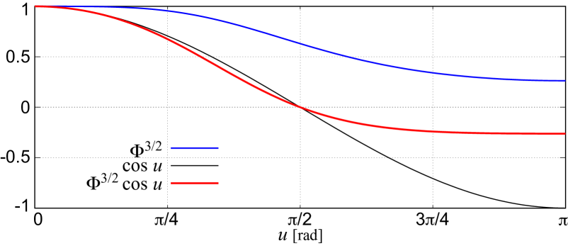
Figure 30: An example plot of $\Phi^{\frac{3}{2}}$, $\cos u$, and $\Phi^{\frac{3}{2}}\cos u$ that shows their dependence on $u$. $\alpha=0.6$ in this plot.

Appendix B von Zeipel’s $\frac{\partial^{2}R}{\partial e^{2}}$ in the Outer Problem

Here we show the actual expressions of the second derivative of the doubly averaged disturbing function $R$ for the outer CR3BP by eccentricity $e$ up to $O\bigl{(}{\alpha^{\prime}}^{5}\bigr{)}$ when $\cos 2g=\pm 1$. This is omitted in our Eq. (353) on p. 353. Our calculation is based on the expressions of $R^{\prime}_{3}$ and $R^{\prime}_{5}$ in Eq. (Z98-323). When $\cos 2g=+1$, the derivative is

$$\frac{\partial^{2}R}{\partial e{}^{2}}=\left.\frac{\partial^{2}}{\partial e{}^{2}}\left(R^{\prime}_{3}{\alpha^{\prime}}^{3}+R^{\prime}_{5}{\alpha^{\prime}}^{5}\right)\right|_{\cos 2g=+1}$$ (420)

$$=\frac{1}{1024\left(1-e^{2}\right)^{\frac{15}{2}}}\left.\Bigl{\{}\left[-1536e^{10}\right.\right.$$

$$+\left(-11520k^{2}+5760\right)e^{8}+\left(32640k^{2}-7680\right)e^{6}$$

$$\quad+\left(-28800k^{2}+3840\right)e^{4}$$

$$\quad\quad\left.+5760k^{2}e^{2}+1920k^{2}-384\right]{\alpha^{\prime}}^{3}$$

$$+\left[-270e^{8}+\left(5040k^{2}+3285\right)e^{6}\right.$$

$$\quad+\left(28350k^{4}+47250k^{2}-5400\right)e^{4}$$

$$\quad\quad+\left(99225k^{4}-47250k^{2}+2025\right)e^{2}$$

$$\quad\quad\quad\left.\left.+7560k^{4}-5040k^{2}+360\right]{\alpha^{\prime}}^{5}\right\}.$$

When $\cos 2g=-1$, it is

$$\frac{\partial^{2}R}{\partial e{}^{2}}=\left.\frac{\partial^{2}}{\partial e{}^{2}}\left(R^{\prime}_{3}{\alpha^{\prime}}^{3}+R^{\prime}_{5}{\alpha^{\prime}}^{5}\right)\right|_{\cos 2g=-1}$$ (421)

$$=\frac{1}{1024\left(1-e^{2}\right)^{\frac{15}{2}}}\left.\Bigl{\{}\left[-1536e^{10}\right.\right.$$

$$+\left(-11520k^{2}+5760\right)e^{8}+\left(32640k^{2}-7680\right)e^{6}$$

$$\quad+\left(-28800k^{2}+3840\right)e^{4}$$

$$\quad\quad\left.+5760k^{2}e^{2}+1920k^{2}-384\right]{\alpha^{\prime}}^{3}$$

$$+\left[5130e^{8}+(85680k^{2}-1935)e^{6}\right.$$

$$\quad+(141750k^{4}+25650k^{2}-10800)e^{4}$$

$$\quad\quad+(163485k^{4}-103410k^{2}+6885)e^{2}$$

$$\quad\quad\quad\left.\left.+10080k^{4}-7920k^{2}+720\right]{\alpha^{\prime}}^{5}\right\}.$$

As we see, the terms at $O\bigl{(}{\alpha^{\prime}}^{3}\bigr{)}$ are common between Eq. (420) and Eq. (421). Now substituting $e=e^{\prime}_{2.0}$ of Eq. (Z103-340) into Eq. (420), $\frac{\partial^{2}R}{\partial e{}^{2}}$ becomes as follows at $\left(\pm e^{\prime}_{2.0},0\right)$ up to $O\bigl{(}{\alpha^{\prime}}^{5}\bigr{)}$:

$$\left.\frac{\partial^{2}R}{\partial e{}^{2}}\right|_{(\pm e^{\prime}_{2.0},0)} \!\!\!=-\frac{3\sqrt{5}\left(5k^{2}-1\right)}{2500k^{\frac{7}{2}}}{\alpha^{\prime}}^{3}$$ (422)

$$\!\!\!\,\,+\frac{9\sqrt{5}\left(425k^{4}-210k^{2}+49\right)}{5000000k^{\frac{11}{2}}}{\alpha^{\prime}}^{5}.$$

Similarly, substituting $e=e^{\prime}_{0.2}$ of Eq. (Z104-341) into Eq. (421), $\frac{\partial^{2}R}{\partial e{}^{2}}$ becomes as follows at $\left(0,\pm e^{\prime}_{0.2}\right)$:

$$\left.\frac{\partial^{2}R}{\partial e{}^{2}}\right|_{(0,\pm e^{\prime}_{0.2})} \!\!\!=-\frac{3\sqrt{5}\left(5k^{2}-1\right)}{2500k^{\frac{7}{2}}}{\alpha^{\prime}}^{3}$$ (423)

$$\!\!\!\,\,+\frac{9\sqrt{5}\left(1375k^{4}-520k^{2}+81\right)}{5000000k^{\frac{11}{2}}}{\alpha^{\prime}}^{5}.$$

The first terms on the right-hand side of Eqs. (422) and (423) remain positive while $k^{2}<\frac{1}{5}$. It is also easy to confirm that the second terms of both the equations are positive in the entire region of $0\leq k^{2}\leq 1$ (see Fig. 31 for a simple illustration). Therefore, the conclusion we stated (hence von Zeipel stated) as Eq. (354), i.e. $\frac{\partial^{2}R}{\partial e{}^{2}}>0$, stands true even when the terms of $O\bigl{(}{\alpha^{\prime}}^{5}\bigr{)}$ are taken into account.

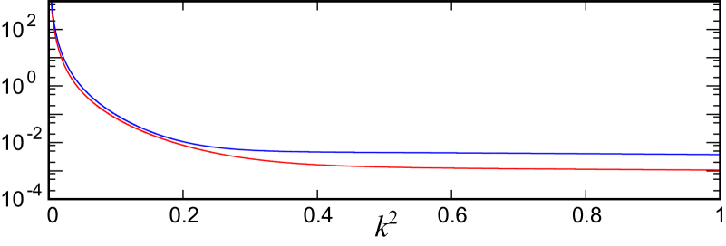
Figure 31: Red: the second term in Eq. (422). Blue: the second term in Eq. (423). $\alpha^{\prime}=1$ is assumed for both the terms. See Supplementary Information 6 for more expository figures.

Appendix for arXiv

In the spring of 2022, the publisher of this monograph (Terrapub) went bankrupt and the official website disappeared (http://www.terrapub.co.jp/). Since there is no printed version of this monograph series, there is currently no way to access any of the papers published in this monograph. Naturally, the DOI for our paper is also not linked anywhere (10.5047/meep.2019.00701.0001). We have no idea if this publisher’s website will be restored or when the DOI information will be corrected.

As a temporary solution to this problem, we have placed the PDF files of the main text and its supplementary material of this paper at the following sites so that interested readers can access our paper.

• ResearchGate

  • main text and supplementary information

• The author’s homepage

  • a whole archive of the publisher’s webpage

    • PDF main text

    • PDF supplementar information

• Figshare

  • pointers to the above material

References

- Abt (1999) Abt, H. A. (editor) (1999), The Astrophysical Journal: American Astronomical Society Centennial Issue—Selected Fundamental Papers Published this Century in the Astronomical Journal and the Astrophysical Journal, University of Chicago Press, Chicago, [ http://press.uchicago.edu/ucp/books/book/distributed/A/bo3644926.html ], also published as The Astrophysical Journal vol. 525C, Number 1C, Part 3, 934–935.
- Alemi (2009) Alemi, A. (2009), Laplace–Runge–Lenz Vector, Report to CDS205 (ComputingMathematical Sciences), Division of Engineering & Applied Science, Caltech, [ http://www.cds.caltech.edu/~marsden/wiki/uploads/projects/geomech/Alemicds205final.pdf ].
- Amore and Aranda (2005) Amore, P., and A. Aranda (2005), Improved Lindstedt–Poincaré method for the solution of nonlinear problems, Journal of Sound and Vibration, 283, 1115–1136, [ https://doi.org/10.1016/j.jsv.2004.06.009 ].
- Antognini (2015) Antognini, J. M. O. (2015), Timescales of Kozai–Lidov oscillations at quadrupole and octupole order in the test particle limit, Monthly Notices of the Royal Astronomical Society, 452, 3610–3619, [ https://doi.org/10.1093/mnras/stv1552 ].
- Antognini (2016) Antognini, J. M. O. (2016), Adventures in the Kozai–Lidov Mechanism, Ph.D. thesis, Graduate Program in Astronomy, The Ohio State University, [ http://rave.ohiolink.edu/etdc/view?acc_num=osu1450697815 ], pp. 169.
- Askey (2005) Askey, R. (2005), The 1839 paper on permutations: Its relation to the Rodrigues formula and further developments, in Mathematics and Social Utopias in France: Olinde Rodrigues and His Times, edited by Altmann, S., and E. L. Ortiz, number 28 in History of Mathematics, 105–118, American Mathematical Society, Providence, Rhode Island, [ http://www.ams.org/publications/authors/books/postpub/hmath-28 ].
- Babadzhanov and Obrubov (1992) Babadzhanov, P. B., and Yu. V. Obrubov (1992), Evolution of short period meteoroid streams, Celestial Mechanics and Dynamical Astronomy, 54, 111–127, [ https://doi.org/10.1007/BF00049547 ].
- Babadzhanov et al. (2015) Babadzhanov, P. B., G. I. Kokhirova, and Iu. V. Obrubov (2015), The potentially hazardous asteroid 2007CA19 as the parent of the -Virginids meteoroid stream, Astronomy and Astrophysics, 579, A119, [ https://doi.org/10.1051/0004-6361/201424923 ].
- Babadzhanov et al. (2017) Babadzhanov, P. B., G. I. Kokhirova, I. P. Williams, and Iu. V. Obrubov (2017), Investigation into the relationship between comet 96P/Machholz 1 and asteroid 2003 EH1, Astronomy and Astrophysics, 598, A94, [ https://doi.org/10.1051/0004-6361/201629006 ].
- Bailey (1983) Bailey, M. E. (1983), Is there a dense primordial cloud of comets just beyond Pluto?, in Proceedings of Asteroids, Comets, Meteors,, 383–386, Uppsala Universitet, Uppsala, Sweden, June 20–22, [ http://ads.nao.ac.jp/abs/1983acm..proc..383B ].
- Bailey and Emel’yanenko (1996) Bailey, M. E., and V. V. Emel’yanenko (1996), Dynamical evolution of Halley-type comets, Monthly Notices of the Royal Astronomical Society, 278, 1087–1110, [ https://doi.org/10.1093/mnras/278.4.1087 ].
- Bailey et al. (1992) Bailey, M. E., J. E. Chambers, and G. Hahn (1992), Origin of sungrazers: a frequent cometary end-state, Astronomy and Astrophysics, 257, 315–322, [ http://ads.nao.ac.jp/abs/1992A%26A...257..315B ].
- Bannister et al. (2016) Bannister, M. T., J. J. Kavelaars, J.-M. Petit, B. J. Gladman, S. D. J. Gwyn, Y.-T. Chen, K. Volk, M. Alexandersen, S. D. Benecchi, A. Delsanti, W. C. Fraser, M. Granvik, W. M. Grundy, A. Guilbert-Lepoutre, D. Hestroffer, W.-H. Ip, R. Marian Jakubik, L. Jones, N. Kaib, C. F, K. P. Lacerda, S. Lawler, M. J. Lehner, H. W. Lin, T. Lister, P. S. Lykawka, S. Monty, M. Marsset, R. Murray-Clay, K. S. Noll, A. Parker, R. E. Pike, P. Rousselot, D. Rusk, M. E. Schwamb, C. Shankman, B. Sicardy, P. Vernazza, and S.-Y. Wang (2016), The outer solar system origins survey. I. Design and first-quarter discoveries, The Astronomical Journal, 152, 70, [ https://doi.org/10.3847/0004-6256/152/3/70 ].
- Barrow-Green (1996) Barrow-Green, J. (1996), Poincaré and the Three Body Problem, number 11 in History of Mathematics, American Mathematical Society, Providence, RI, USA, [ https://bookstore.ams.org/hmath-11 ].
- Battin (1987) Battin, R. H. (1987), An Introduction to the Mathematics and Methods of Astrodynamics, American Institute of Aeronautics and Astronautics, Inc., New York, [ https://doi.org/10.2514/4.861543 ].
- Batygin (2018) Batygin, K. (2018), Yoshihide Kozai (1928–2018), Guest Blogs, Planetary Society, [ http://www.planetary.org/blogs/guest-blogs/2018/0227-yoshihide-kozai-1928-2018.html ].
- Batygin and Laughlin (2008) Batygin, K., and G. Laughlin (2008), On the dynamical stability of the solar system, The Astrophysical Journal, 683, 1207–1216, [ https://doi.org/10.1086/589232 ].
- Batygin et al. (2015) Batygin, K., A. Morbidelli, and M. J. Holman (2015), Chaotic disintegration of the inner solar system, The Astrophysical Journal, 799, 120, [ https://doi.org/10.1088/0004-637X/799/2/120 ].
- Beekman (2005) Beekman, G. (2005), The nearly forgotten scientist Ivan Osipovich Yarkovsky, Journal of the British Astronomical Association, 115, 207–212, [ http://ads.nao.ac.jp/abs/2005JBAA..115..207B ].
- Beekman (2006) Beekman, G. (2006), I. O. Yarkovsky and the discovery of ‘his’ effect, Journal of Historical Astronomy, 37, 71–86, [ https://doi.org/10.1177/002182860603700106 ].
- Beletsky (1972) Beletsky, V. V. (1972), Essays on the Motion of Celestial Bodies, Nauka, Moscow, [ http://www.twirpx.com/file/459250/ ], originally in Russian, translated in English as Beletsky (2001).
- Beletsky (2001) Beletsky, V. V. (2001), Essays on the Motion of Celestial Bodies, Springer Basel AG, Dordrecht, [ http://link.springer.com/book/10.1007%2F978-3-0348-8360-3 ], an English translation of Beletsky (1972) by Andrei Iacob.
- Berliner Astronomisches Jahrbuch für 1911 (Published in 1909) Berliner Astronomisches Jahrbuch für 1911 (Published in 1909), 136. Jahrgang, Königliches Astronomisches Recheninstitut unter Leitung von J. Bauschinger (Berlin: Ferd. Dümmlers Verlagsbuchhandlung (Kommissionsverlag)), [ https://jbc.bj.uj.edu.pl/dlibra/publication/382324/edition/363926 ].
- Beust and Dutrey (2006) Beust, H., and A. Dutrey (2006), Dynamics of the young multiple system GG Tauri. II. Relation between the stellar system and the circumbinary disk, Astronomy and Astrophysics, 446, 137–154, [ https://doi.org/10.1051/0004-6361:20053163 ].
- Birkhoff (1913) Birkhoff, G. D. (1913), Proof of Poincaré’s geometric theorem, Transactions of the American Mathematical Society, 14, 14–22, [ https://doi.org/10.2307/1988766 ], a Japanese translation is available from http://th.nao.ac.jp/~tanikawa/list01/list012.html.
- Birkhoff (1915) Birkhoff, G. D. (1915), The restricted problem of three bodies, Rendiconti del Circolo Matematico di Palermo (1884–1940), 39, 265–334, [ https://doi.org/10.1007/BF03015982 ].
- Birkhoff (1922) Birkhoff, G. D. (1922), Surface transformations and their dynamical applications, Acta Mathematica, 43, 1–119, [ https://doi.org/10.1007/BF02401754 ].
- Birkhoff (1926) Birkhoff, G. D. (1926), An extension of Poincaré’s last geometric theorem, Acta Mathematica, 47, 297–311, [ https://doi.org/10.1007/BF02559515 ], a Japanese translation is available from http://th.nao.ac.jp/~tanikawa/list01/list013.html.
- Boccaletti and Pucacco (1996) Boccaletti, D., and G. Pucacco (1996), Theory of Orbits. 1. Integrable systems and non-perturbative methods, Springer–Verlag, Berlin, [ http://www.springer.com/us/book/9783540589631 ].
- Boccaletti and Pucacco (1998) Boccaletti, D., and G. Pucacco (1998), Theory of Orbits. 2. Perturbative and geometrical methods, Springer–Verlag, Berlin, [ http://www.springer.com/la/book/9783540603559 ].
- Boekholt et al. (2016) Boekholt, T. C. N., F. I. Pelupessy, D. C. Heggie, and S. F. Portegies Zwart (2016), The origin of chaos in the orbit of comet 1P/Halley, Monthly Notices of the Royal Astronomical Society, 461, 3576–3584, [ https://doi.org/10.1093/mnras/stw1504 ].
- Bohlin (1888) Bohlin, K. (1888), Über eine neue Annäherungsmethode in der Störungstheorie, Bihang till Kongl. Svenska Vetenskaps–Akademiens Handlingar, 14, 1–26.
- Bottke et al. (2001) Bottke, W. F., D. Vokrouhlický, M. Brož, D. Nesvorný, and A. Morbidelli (2001), Dynamical spreading of asteroid families by the Yarkovsky effect, Science, 294, 1693–1696, [ https://doi.org/10.1126/science.1066760 ].
- Bottke et al. (2002a) Bottke, W. F., A. Morbidelli, R. Jedicke, J. M. Petit, H. F. Levison, P. Michel, and T. S. Metcalfe (2002a), Debiased orbital and absolute magnitude distribution of the near-Earth objects, Icarus, 156, 399–433, [ https://doi.org/10.1006/icar.2001.6788 ].
- Bottke et al. (2002b) Bottke, W. F., D. Vokrouhlický, D. P. Rubincam, and M. Brož (2002b), The effect of Yarkovsky thermal forces on the dynamical evolution of asteroids and meteoroids, in Asteroids III, edited by Bottke, W. F., A. Cellino, P. Paolicchi, and R. P. Binzel, 395–408, The University of Arizona Press, Tucson, Arizona, [ http://ads.nao.ac.jp/abs/2002aste.book..395B ].
- Bottke et al. (2006) Bottke, W. F., D. Nesvorný, D. P. Rubincam, and D. Vokrouhlický (2006), The Yarkovsky and YORP effects: Implications for asteroid dynamics, Annual Reviews of Earth and Planetary Science, 34, 157–191, [ https://doi.org/10.1146/annurev.earth.34.031405.125154 ].
- Bottke et al. (2010) Bottke, W. F., D. Nesvorný, D. Vokrouhlický, and A. Morbidelli (2010), The irregular satellites: The most collisionally evolved populations in the solar system, The Astronomical Journal, 139, 994–1014, [ https://doi.org/10.1088/0004-6256/139/3/994 ].
- Brasil et al. (2014) Brasil, P. I. O., R. S. Gomes, and J. S. Soares (2014), Dynamical formation of detached trans-Neptunian objects close to the 2:5 and 1:3 mean motion resonances with Neptune, Astronomy and Astrophysics, 564, A44, [ https://doi.org/10.1051/0004-6361/201322041 ].
- Breiter and Ratajczak (2005) Breiter, S., and R. Ratajczak (2005), Vectorial elements for the Galactic disc tide effects in cometary motion, Monthly Notices of the Royal Astronomical Society, 364, 1222–1228, [ https://doi.org/10.1111/j.1365-2966.2005.09658.x ].
- Broucke (1981) Broucke, R. A. (1981), Expansion of the third-body disturbing function, Journal of Guidance, Control, and Dynamics, 4, 346–348, [ https://doi.org/10.2514/3.19740 ].
- Brouwer (1947) Brouwer, D. (1947), Secular variations of the elements of Encke’s comet, The Astronomical Journal, 52, 190–198, [ https://doi.org/10.1086/105991 ].
- Brouwer and Clemence (1961) Brouwer, D., and G. M. Clemence (1961), Methods of Celestial Mechanics, Academic Press, New York, [ http://www.sciencedirect.com/science/book/9781483200750 ].
- Brown and Shook (1933) Brown, E. W., and C. A. Shook (1933), Planetary Theory, Cambridge University Press, Cambridge, UK, [ https://archive.org/details/planetarytheory032086mbp ], republished by Dover in 1964, New York.
- Bruns (1887) Bruns, H. (1887), Über die Integrale des Vielkörper-Problems, Acta Mathematica, 11, 25–96, [ https://projecteuclid.org/euclid.acta/1485881150 ].
- Burns et al. (1979) Burns, J. A., P. L. Lamy, and S. Soter (1979), Radiation forces on small particles in the solar system, Icarus, 40, 1–48, [ https://doi.org/10.1016/0019-1035(79)90050-2 ].
- Burns et al. (2014) Burns, J. A., P. L. Lamy, and S. Soter (2014), Radiation forces on small particles in the Solar System: A re-consideration, Icarus, 232, 263–265, [ https://doi.org/10.1016/j.icarus.2013.12.028 ].
- Bush (1992) Bush, A. W. (1992), Perturbation Methods for Engineers and Scientists, Library of Engineering Mathematics, CRC Press, Boca Raton, Ann Arbor, London, Tokyo, [ https://books.google.co.jp/books/about/Perturbation_Methods_for_Engineers_and_S.html?id=txDro37uTvwC&redir_esc=y ].
- Caidin (1963) Caidin, M. (1963), Red Star in Space, The Crowell–Collier Press, New York, [ https://www.amazon.com/dp/B0006D9DBI ].
- Callandreau (1902) Callandreau, O. (1902), Revue des publications astronomiques, Bulletin Astronomique, 19, 286, [ https://gallica.bnf.fr/ark:/12148/bpt6k65369785 ], a brief introduction of von Zeipel (1901).
- Cameron (1962) Cameron, A. G. W. (1962), The formation of the sun and planets, Icarus, 1, 13–69, [ https://doi.org/10.1016/0019-1035(62)90005-2 ].
- Carvalho et al. (2013) Carvalho, J. P. S., R. V. de Moraes, A. F. B. A. Prado, and O. C. Winter (2013), Analysis of the secular problem for triple star systems, Journal of Physics: Conference Series, 465, 012010, [ https://doi.org/10.1088/1742-6596/465/1/012010 ].
- Charlier (1902) Charlier, C. L. (1902), Die Mechanik des Himmels (erster band), Verlag von Veit & Comp., Leipzig, [ https://archive.org/details/diemechanikdesh00unkngoog ].
- Charlier (1907) Charlier, C. L. (1907), Die Mechanik des Himmels (zweiter band), Verlag von Veit & Comp., Leipzig, [ https://archive.org/details/diemechanikdeshi02charuoft ].
- Chenciner (2015) Chenciner, A. (2015), Poincaré and the Three-Body Problem, in Henri Poincaré, 1912–2012, 51–149, Birkhäuer Basel, [ https://doi.org/10.1007/978-3-0348-0834-7_2 ].
- Chesley et al. (2003) Chesley, S. R., S. J. Ostro, D. Vokrouhlický, D. Čapek, J. D. Girgini, M. C. Nolan, J. L. Margot, A. A. Hine, L. A. M. Benner, and A. B. Chamberlin (2003), Direct detection of the Yarkovsky effect by radar ranging to asteroid 6489 Golevka, Science, 302, 1739–1742, [ https://doi.org/10.1126/science.1091452 ].
- Chirikov and Vecheslavov (1989) Chirikov, R. V., and V. V. Vecheslavov (1989), Chaotic dynamics of comet Halley, Astronomy and Astrophysics, 221, 146–154, [ http://ads.nao.ac.jp/abs/1989A%26A...221..146C ].
- Cody (1965a) Cody, W. J. (1965a), Chebyshev approximations for the complete elliptic integrals and , Math. Comp., 19, 105–112, [ https://doi.org/10.1090/S0025-5718-1965-0171370-4 ].
- Cody (1965b) Cody, W. J. (1965b), Chebyshev polynomial expansions of complete elliptic integrals and , Math. Comp., 19, 249–259, [ https://doi.org/10.1090/S0025-5718-1965-0178563-0 ].
- Collas (1970) Collas, P. (1970), Algebraic solution of the Kepler problem using the Runge–Lenz vector, American Journal of Physics, 38, 253–255, [ https://doi.org/10.1119/1.1976296 ].
- Ćuk and Burns (2004) Ćuk, M., and J. A. Burns (2004), On the secular behavior of irregular satellites, The Astronomical Journal, 128, 2518–2541, [ https://doi.org/10.1086/424937 ].
- Dahl (1968) Dahl, J. (1968), Physical interpretation of the Runge–Lenz vector, Physics Letters A, 27, 62–63, [ https://doi.org/10.1016/0375-9601(68)91339-X ].
- Danby (1992) Danby, J. M. A. (1992), Fundamentals of Celestial Mechanics, Willmann–Bell Inc., Richmond, Virginia, [ http://www.willbell.com/math/mc7.htm ], 2nd edition.
- Davies et al. (2008) Davies, J. K., J. McFarland, M. E. Bailey, B. G. Marsden, and W. H. Ip (2008), The early development of ideas concerning the transneptunian region, in The Solar System Beyond Neptune, edited by Barucci, M. A., H. Boehnhardt, D. P. Cruikshank, and A. Morbidelli, 11–23, The University of Arizona Press, Tucson, Arizona, [ https://www.lpi.usra.edu/books/ssbn2008/download.html ].
- Davies et al. (2014) Davies, M. B., F. C. Adams, P. Armitage, J. Chambers, E. Ford, A. Morbidelli, S. N. Raymond, and D. Veras (2014), The long-term dynamical evolution of planetary systems, Protostars and Planets VI, 787–808, [ https://doi.org/10.2458/azu_uapress_9780816531240-ch034 ].
- de Elía et al. (2019) de Elía, G. C., M. Zanardi, A. Dugaro, and S. Naoz (2019), Inverse Lidov–Kozai resonance for an outer test particle due to an eccentric perturber, Astronomy and Astrophysics, 627, A17, [ https://doi.org/10.1051/0004-6361/201935220 ].
- de la Fuente Marcos and de la Fuente Marcos (2018) de la Fuente Marcos, C., and R. de la Fuente Marcos (2018), Kozai–Lidov resonant behavior among Atira-class asteroids, Research Notes of the American Astronomical Society, 2, 46, [ https://doi.org/10.3847/2515-5172/aac9ce ].
- Delaunay (1860) Delaunay, C. E. (1860), Théorie du mouvement de la Lune, tome premier, number 28 in Mémoires de l’académie des sciences de l’institut impérial de France, Mallet–Bachelier, Paris, [ https://books.google.co.jp/books?id=KS09AQAAIAAJ ].
- Delaunay (1867) Delaunay, C. E. (1867), Théorie du mouvement de la Lune, deuxiéme volume, number 29 in Mémoires de l’académie des sciences de l’institut impérial de France, Gauthier–Villars, Paris, [ https://books.google.co.jp/books?id=NMdHAQAAMAAJ ].
- Delbo et al. (2014) Delbo, M., G. Libourel, J. Wilkerson, N. Murdoch, P. Michel, K. T. Ramesh, C. Ganino, C. Verati, and S. Marchi (2014), Thermal fatigue as the origin of regolith on small asteroids, Nature, 508, 233–236, [ https://doi.org/10.1038/nature13153 ].
- Demidovich and Maron (1966) Demidovich, B. P., and I. A. Maron (1966), Basics of Computational Mathematics, Nauka, Moscow, [ https://www.twirpx.com/file/1491138/ ], originally in Russian, translated in English as Demidovich and Maron (1981).
- Demidovich and Maron (1981) Demidovich, B. P., and I. A. Maron (1981), Computational Mathematics, Mir Publishers, Moscow, [ https://trove.nla.gov.au/work/10233601 ], an English translation of Demidovich and Maron (1966) by George Yankovsky.
- Deprit (1969) Deprit, A. (1969), Canonical transformations depending on a small parameter, Celestial Mechanics, 1, 12–30, [ https://doi.org/10.1007/BF01230629 ].
- DeVorkin (1997) DeVorkin, D. (1997), Interview of Yoshihide Kozai, Niels Bohr Library & Archives, American Institute of Physics, College Park, MD USA, recorded on 1997 September 2, [ http://www.aip.org/history-programs/niels-bohr-library/oral-histories/24816 ].
- Diacu and Holmes (1996) Diacu, F., and P. Holmes (1996), Celestial Encounters: The Origins of Chaos and Stability, Princeton University Press, Princeton, New Jersey, [ https://press.princeton.edu/titles/5913.html ].
- Domingos et al. (2013) Domingos, R. C., A. F. B. A. Prado, and R. V. de Moraes (2013), A study of single- and double-averaged second-order models to evaluate third-body perturbation considering elliptic orbits for the perturbing body, Mathematical Problems in Engineering, 2013, 111, [ https://doi.org/10.1155/2013/260830 ].
- Duplantier and Rivasseau (2015) Duplantier, B., and V. Rivasseau (editors) (2015), Henri Poincaré, 1912–2012, volume 67 of Progress in Mathematical Physics, Birkhäuer Basel, [ https://doi.org/10.1007/978-3-0348-0834-7 ].
- Edgeworth (1943) Edgeworth, K. E. (1943), The evolution of our solar system, Journal of the British Astronomical Association, 53, 181–188, [ http://ads.nao.ac.jp/abs/1943JBAA...53..181E ].
- Edgeworth (1949) Edgeworth, K. E. (1949), The origin and evolution of the solar system, Monthly Notices of the Royal Astronomical Society, 109, 600–609, [ http://ads.nao.ac.jp/abs/1949MNRAS.109..600E ].
- Egorov (2001) Egorov, V. A. (2001), Recollections about M. L. Lidov, Cosmic Research, 39, 421–423, [ https://doi.org/10.1023/A:1012380726949 ], originally in Russian.
- Ellis and Murray (2000) Ellis, K., and C. D. Murray (2000), The disturbing function in solar system dynamics, Icarus, 147, 129–144, [ https://doi.org/10.1006/icar.2000.6399 ].
- Elshaboury and Mostafa (2013) Elshaboury, S. M., and A. Mostafa (2013), The singly averaged elliptical restricted three-body problem, Astrophysics and Space Science, 348, 385–391, [ https://doi.org/10.1007/s10509-013-1586-z ].
- Emel’yanenko (2017) Emel’yanenko, V. V. (2017), Near-Sun asteroids, Solar System Research, 51, 59–63, [ https://doi.org/10.1134/S0038094616060010 ], originally in Russian.
- Fabrycky and Tremaine (2007) Fabrycky, D., and S. Tremaine (2007), Shrinking binary and planetary orbits by Kozai cycles with tidal friction, The Astrophysical Journal, 669, 1298–1315, [ https://doi.org/10.1086/521702 ].
- Farago and Laskar (2010) Farago, F., and J. Laskar (2010), High-inclination orbits in the secular quadrupolar three-body problem, Monthly Notices of the Royal Astronomical Society, 401, 1189–1198, [ https://doi.org/10.1111/j.1365-2966.2009.15711.x ].
- Farinella and Vokrouhlický (1999) Farinella, P., and D. Vokrouhlický (1999), Semimajor axis mobility of asteroidal fragments, Science, 283, 1507–1510, [ https://doi.org/10.1126/science.283.5407.1507 ].
- Farinella et al. (1998) Farinella, P., D. Vokrouhlický, and W. K. Hartmann (1998), Meteorite delivery via Yarkovsky orbital drift, Icarus, 132, 378–387, [ https://doi.org/10.1006/icar.1997.5872 ], erratum is available in https://doi.org/10.1006/icar.1998.6004.
- Farinella et al. (2001) Farinella, P., L. Foschini, Ch. Froeschlé, R. Gonczi, T. J. Jopek, G. Longo, and P. Michel (2001), Probable asteroidal origin of the Tunguska cosmic body, Astronomy and Astrophysics, 377, 1081–1097, [ https://doi.org/10.1051/0004-6361:20011054 ].
- Fatou (1931) Fatou, P. (1931), Sur le mouvement d’un point matérial ans un champ de gravitation fixe, Acta Astronomica, 2, 101–164.
- Felsentreger (1968) Felsentreger, T. L. (1968), Classification of lunar satellite orbits, Planetary and Space Science, 16, 285–295, [ https://doi.org/10.1016/0032-0633(68)90003-2 ].
- Ford et al. (2000) Ford, E. B., B. Kozinsky, and F. A. Rasio (2000), Secular evolution of hierarchical triple star systems, The Astrophysical Journal, 535, 385–401, [ https://doi.org/10.1086/308815 ], erratum is available in https://doi.org/10.1086/382349.
- Fouchard et al. (2005) Fouchard, M., Ch. Froeschlé, J. J. Matese, and G. B. Valsecchi (2005), Comparison between different models of galactic tidal effects on cometary orbits, Celestial Mechanics and Dynamical Astronomy, 93, 229–262, [ https://doi.org/10.1007/s10569-005-1149-x ], erratum is available in https://doi.org/10.1007/s10569-006-9055-4.
- Froeschlé et al. (1991) Froeschlé, Ch., A. Morbidelli, and H. Scholl (1991), Complex dynamical behaviour of the asteroid 2335 James associated with the secular resonances and : numerical studies and theoretical interpretation, Astronomy and Astrophysics, 249, 553–562, [ http://ads.nao.ac.jp/abs/1991A%26A...249..553F ].
- de la Fuente Marcos et al. (2014) de la Fuente Marcos, C., R. de la Fuente Marcos, and S. J. Aarseth (2014), Flipping minor bodies: What comet 96P/Machholz 1 can tell us about the orbital evolution of extreme trans-Neptunian objects and the production of near-Earth objects on retrograde orbits, Monthly Notices of the Royal Astronomical Society, 446, 1867–1873, [ https://doi.org/10.1093/mnras/stu2230 ].
- Galassi et al. (2009) Galassi, M., J. Davies, J. Theiler, B. Gough, G. Jungman, P. Alken, M. Booth, and F. Rossi (2009), GNU Scientific Library Reference Manual, 3rd edition, [ http://www.gnu.org/software/gsl/ ].
- Gallardo (2006) Gallardo, T. (2006), The occurrence of high-order resonances and Kozai mechanism in the scattered disk, Icarus, 181, 205–207, [ https://doi.org/10.1016/j.icarus.2005.11.011 ].
- Gallardo et al. (2012) Gallardo, T., G. Hugo, and P. Pais (2012), Survey of Kozai dynamics beyond Neptune, Icarus, 220, 392–403, [ https://doi.org/10.1016/j.icarus.2012.05.025 ].
- Galle (1894) Galle, J. G. (1894), Verzeichniss der Elemente der bisher berechneten Cometenbahnen nebst Anmerkungen und Literatur-Nachweisen neu bearbeitet, ergänzt und fortgesetzt bis zum Jahre 1894, Verlag von Wilhelm Engelmann, Leipzig, [ https://archive.org/details/verzeichnissder01gallgoog ].
- Gårding (1998) Gårding, L. (1998), Mathematics and Mathematicians: Mathematics in Sweden before 1950, number 13 in History of Mathematics, American Mathematical Society and London Mathematical Society, Providence, Rhode Island, [ http://bookstore.ams.org/hmath-13/ ], originally published in Swedish by Lund University Press, Lund, Sweden, 1994, translated from Swedish into English by Lars Gårding.
- Gentile and Mastropietro (1999) Gentile, G., and V. Mastropietro (1999), Methods for the analysis of the Lindstedt series for KAM tori and renormalizability in classical mechanics: A review with some applications, Reviews in Mathematical Physics, 8, 393–444, [ https://doi.org/10.1142/S0129055X96000135 ].
- German (2010) German, R. M. (2010), Coarsening in sintering: Grain shape distribution, grain size distribution, and grain growth kinetics in solid-pore systems, Critical Reviews in Solid State and Materials Sciences, 35, 263–305, [ https://doi.org/10.1080/10408436.2010.525197 ].
- Giacaglia (1968) Giacaglia, G. E. O. (1968), Secular motion of resonant asteroids, SAO Special Report 278, Smithsonian Institution, Astrophysical Observatory, Cambridge, Massachusetts, USA, [ http://ads.nao.ac.jp/abs/1968SAOSR.278.....G ].
- Giacaglia (1969) Giacaglia, G. E. O. (1969), Resonance in the restricted problem of three bodies, The Astronomical Journal, 74, 1254–1261, [ https://doi.org/10.1086/110930 ].
- Gladman et al. (2008) Gladman, B., B. G. Marsden, and C. VanLaerhoven (2008), Nomenclature in the outer solar system, in The Solar System Beyond Neptune, edited by Barucci, M. A., H. Boehnhardt, D. P. Cruikshank, and A. Morbidelli, 43–57, The University of Arizona Press, Tucson, Arizona, [ http://ads.nao.ac.jp/abs/2008ssbn.book...43G ].
- Goldstein (1975) Goldstein, H. (1975), Prehistory of the “Runge–Lenz” vector, American Journal of Physics, 43, 737–738, [ https://doi.org/10.1119/1.9745 ].
- Goldstein (1976) Goldstein, H. (1976), More on the prehistory of the Laplace or Runge–Lenz vector, American Journal of Physics, 44, 1123–1124, [ https://doi.org/10.1119/1.10202 ].
- Goldstein (1980) Goldstein, H. (1980), Classical Mechanics, Addison Wesley, Boston, Massachusetts, USA, [ https://www.pearson.com/us/higher-education/product/9780201029185.html ], 2nd edition.
- Goldstein et al. (2002) Goldstein, H., C. Poole, and J. Safko (2002), Classical Mechanics, Addison Wesley, Boston, Massachusetts, USA, [ https://www.pearson.com/us/higher-education/program/PGM170105.html ], 3rd edition.
- Gomes (2011) Gomes, R. S. (2011), The origin of TNO 2004 XR190 as a primordial scattered object, Icarus, 215, 661–668, [ https://doi.org/10.1016/j.icarus.2011.08.002 ].
- Gomes et al. (2005) Gomes, R. S., T. Gallardo, J. A. Fernández, and A. Brunini (2005), On the origin of the high-perihelion scattered disk: The role of the Kozai mechanism and mean motion resonances, Celestial Mechanics and Dynamical Astronomy, 91, 109–129, [ https://doi.org/10.1007/s10569-004-4623-y ].
- Gomes et al. (2008) Gomes, R. S., J. A. Fernádez, T. Gallardo, and A. Brunini (2008), The scattered disk: Origins, dynamics, and end states, in The Solar System Beyond Neptune, edited by Barucci, M. A., H. Boehnhardt, D. P. Cruikshank, and A. Morbidelli, 259–273, The University of Arizona Press, Tucson, Arizona, [ http://ads.nao.ac.jp/abs/2008ssbn.book..259G ].
- Gordeeva (1968) Gordeeva, Yu. F. (1968), Time-dependence of orbital elements in long-period oscillations in the three-body boundary-value problem, Cosmic Research, 6, 450–453, [ http://ads.nao.ac.jp/abs/1968CosRe...6..450G ], originally in Russian.
- Granvik et al. (2016) Granvik, M., A. Morbidelli, R. Jedicke, B. Bolin, W. F. Bottke, E. Beshore, D. Vokrouhlický, M. Delbò, and P. Michel (2016), Super-catastrophic disruption of asteroids at small perihelion distances, Nature, 530, 303–306, [ https://doi.org/10.1038/nature16934 ].
- Granvik et al. (2018) Granvik, M., A. Morbidelli, R. Jedicke, B. Bolin, W. F. Bottke, E. Beshore, D. Vokrouhlický, D. Nesvorný, and P. Michel (2018), Debiased orbit and absolute-magnitude distributions for near-Earth objects, Icarus, 312, 181–207, [ https://doi.org/10.1016/j.icarus.2018.04.018 ].
- Grebenikov (1962) Grebenikov, E. A. (1962), Conference on general and applied problems of theoretical astronomy, Soviet Astronomy, 6, 440–442, [ http://ads.nao.ac.jp/abs/1962SvA.....6..440G ], originally in Russian.
- Grebenikov (1970) Grebenikov, E. A. (1970), A method for developing an analytic trigonometric theory for the motion of resonance asteroids, Soviet Astronomy, 14, 344–350, [ http://ads.nao.ac.jp/abs/1970SvA....14..344G ], originally in Russian.
- Green (1999) Green, D. W. E. (1999), Book Review: Solar system astronomy in America: Communities, patronage, and interdisciplinary research, 1920–1960, International Comet Quarterly, 21, 44–46, [ http://www.icq.eps.harvard.edu/ICQ109pp44t46.pdf ].
- Green (2004a) Green, D. W. E. (2004a), What is improper about the term “Kuiper belt”? (or, Why name a thing after a man who didn’t believe its existence?), International Comet Quarterly, [ http://www.icq.eps.harvard.edu/kb.html ], no volume or page information is given.
- Green (2004b) Green, D. W. E. (2004b), Fred Lawrence Whipple (1906–2004), International Comet Quarterly, 26, 115–118, [ http://www.icq.eps.harvard.edu/FLW_obitICQ.pdf ].
- Greenstreet et al. (2012) Greenstreet, S., H. Ngo, and B. Gladman (2012), The orbital distribution of near-Earth objects inside Earth’s orbit, Icarus, 217, 355–366, [ https://doi.org/10.1016/j.icarus.2011.11.010 ].
- Grimshaw (1991) Grimshaw, R. (1991), Nonlinear Ordinary Differential Equations, Applied Mathematics and Engineering Science Texts, CRC Press, Boca Raton, London, New York, Washington D. C., [ https://books.google.co.jp/books/about/Nonlinear_Ordinary_Differential_Equation.html?id=yEWlegOzWxMC&redir_esc=y ].
- Gronchi and Milani (1998) Gronchi, G. F., and A. Milani (1998), Averaging on Earth-crossing orbits, Celestial Mechanics and Dynamical Astronomy, 71, 109–136, [ https://doi.org/10.1023/A:1008315321603 ], a Japanese translation is available from http://th.nao.ac.jp/~tanikawa/list08/list086.html. Note that the year of publication of this paper is labeled as “1999” in its p. 109 of both the printed and PDF versions. The volume (vol. 71) from which this paper was published has a publication year labeled “1998/1999” in print. However, the publisher’s online bibliographic information for this paper and the volume currently shows “1998” as the year of publication, which is inconsistent with the printed or PDF version.
- Gronchi and Milani (1999) Gronchi, G. F., and A. Milani (1999), The stable Kozai state for asteroids and comets. With arbitrary semimajor axis and inclination, Astronomy and Astrophysics, 341, 928–935, [ http://ads.nao.ac.jp/abs/1999A%26A...341..928G ].
- Gylden (1891) Gylden, H. (1891), Nouvelles recherches sur les séries employés dans les théories des planetès, Acta Mathematica, 15, 65–189, [ https://archive.org/stream/actamathematica15upps#page/64/mode/2up ], including Préliminaires and Chapitre I. See also http://henripoincarepapers.univ-lorraine.fr/chp/text/gylden-1892-05-02.html.
- Gylden (1893) Gylden, H. (1893), Nouvelles recherches sur les séries employés dans les théories des planetès, Acta Mathematica, 17, 1–168, [ https://archive.org/stream/actamathematica17upps#page/n13/mode/2up ], including Chapitre II and Chapitre III. See also http://henripoincarepapers.univ-lorraine.fr/chp/text/gylden-1892-05-02.html.
- Hamilton (1994) Hamilton, D. P. (1994), A comparison of Lorentz, planetary gravitational, and satellite gravitational resonances, Icarus, 109, 221–240, [ https://doi.org/10.1006/icar.1994.1089 ].
- Hamilton and Krivov (1997) Hamilton, D. P., and A. V. Krivov (1997), Dynamics of distant moons of asteroids, Icarus, 128, 241–249, [ https://doi.org/10.1006/icar.1997.5738 ].
- Harrington (1968) Harrington, R. S. (1968), Dynamical evolution of triple stars, The Astronomical Journal, 73, 190–194, [ https://doi.org/10.1086/110614 ].
- Harvey (2007) Harvey, B. (2007), Soviet and Russian Lunar Exploration, Springer, jointly published with Praxis Publishing, Chichester, UK, [ https://doi.org/10.1007/978-0-387-73976-2 ].
- Hastings, Jr. (1955) Hastings, Jr., C. (1955), Approximations for digital computers, Princeton University Press, Princeton, New Jersey, [ https://press.princeton.edu/titles/1133.html ], assisted by Jeanne T. Hayward and James P. Wong, Jr.
- Hébrard et al. (2011) Hébrard, G., D. Ehrenreich, F. Bouchy, X. Delfosse, C. Moutou, I. Arnold, L. Boisse, X. Bonfils, R. F. Díaz, A. Eggenberger, T. Forveille, A. M. Lagrange, C. Lovis, F. Pepe, C. Perrier, D. Queloz, A. Santerne, N. Santos, D. Ségransan, S. Udry, and A. Vidal-Madjar (2011), The retrograde orbit of the HAT-P-6b exoplanet, Astronomy and Astrophysics, 527, L11, [ https://doi.org/10.1051/0004-6361/201016331 ].
- Heine (1878) Heine, E. (1878), Handbuch der Kugelfunctionen, Theorie und Anwendungen, Erster Band. Theorie der Kugelfunctionen und der verwandten Functionen, Druck und Verlag von G. Reimer, Berlin, [ https://books.google.co.jp/books?id=7HWSa_5rIB4C ].
- Heintz (1974) Heintz, W. H. (1974), Determination of the Runge–Lenz vector, American Journal of Physics, 42, 1078–1082, [ https://doi.org/10.1119/1.1987941 ].
- Heisler and Tremaine (1986) Heisler, J., and S. Tremaine (1986), The influence of the galactic tidal field on the Oort comet cloud, Icarus, 65, 13–26, [ https://doi.org/10.1016/0019-1035(86)90060-6 ].
- Higuchi et al. (2007) Higuchi, A., E. Kokubo, H. Kinoshita, and T. Mukai (2007), Orbital evolution of planetesimals due to the Galactic tide: Formation of the comet cloud, The Astronomical Journal, 134, 1693–1706, [ https://doi.org/10.1086/521815 ].
- Hirayama (1918) Hirayama, K. (1918), Groups of asteroids probably of common origin, The Astronomical Journal, 31, 185–188, [ https://doi.org/10.1086/104299 ].
- Hirayama (1922) Hirayama, K. (1922), Families of asteroids, Japanese Journal of Astronomy and Geophysics, 1, 55–93, [ http://ads.nao.ac.jp/abs/1922JaJAG...1...55H ].
- Hori (1966) Hori, G. (1966), Theory of general perturbations with unspecified canonical variables, Publications of the Astronomical Society of Japan, 18, 287–296, [ http://ads.nao.ac.jp/abs/1966PASJ...18..287H ], a Japanese translation is available from http://th.nao.ac.jp/~tanikawa/airborne/tito-01.html.
- Hori (1967) Hori, G. (1967), Non-linear coupling of two harmonic oscillations, Publications of the Astronomical Society of Japan, 19, 229–241, [ http://ads.nao.ac.jp/abs/1967PASJ...19..229H ].
- Ito (2016) Ito, T. (2016), High-order analytic expansion of disturbing function for doubly averaged circular restricted three-body problem, Advances in Astronomy, 2016, Article ID 8945090, [ https://doi.org/10.1155/2016/8945090 ].
- Ito and Malhotra (2010) Ito, T., and R. Malhotra (2010), Asymmetric impacts of near-Earth asteroids on the Moon, Astronomy and Astrophysics, 519, A63, [ https://doi.org/10.1051/0004-6361/200912901 ].
- Ito and Miyama (2001) Ito, T., and S. M. Miyama (2001), An estimation of upper limit masses of Andromedae planets, The Astrophysical Journal, 552, 372–379, [ https://doi.org/10.1086/320470 ].
- Ito and Tanikawa (1999) Ito, T., and K. Tanikawa (1999), Stability and instability of the terrestrial protoplanet system and their possible roles in the final stage of planet formation, Icarus, 139, 336–349, [ https://doi.org/10.1006/icar.1999.6112 ].
- Ito and Tanikawa (2001) Ito, T., and K. Tanikawa (2001), Stability of terrestrial protoplanet systems and alignment of orbital elements, Publications of the Astronomical Society of Japan, 53, 143–151, [ https://doi.org/10.1093/pasj/53.1.143 ].
- Ito and Tanikawa (2002) Ito, T., and K. Tanikawa (2002), Long-term integrations and stability of planetary orbits in our solar system, Monthly Notices of the Royal Astronomical Society, 336, 483–500, [ https://doi.org/10.1046/j.1365-8711.2002.05765.x ].
- Ito and Tanikawa (2007) Ito, T., and K. Tanikawa (2007), Trends in 20th century celestial mechanics, Publications of the National Astronomical Observatory of Japan, 9, 55–112, [ http://ads.nao.ac.jp/abs/2007PNAOJ...9...55I ].
- Ito et al. (2018) Ito, T., M. Ishiguro, T. Arai, M. Imai, T. Sekiguchi, Y. P. Bach, Y. G. Kwon, M. Kobayashi, R. Ishimaru, H. Naito, M. Watanabe, and K. Kuramoto (2018), Extremely strong polarization of an active asteroid (3200) Phaethon, Nature Communications, 9, 2486, [ https://doi.org/10.1038/s41467-018-04727-2 ].
- Ivezić et al. (2001) Ivezić, Ž., S. Tabachnik, R. Rafikov, R. H. Lupton, T. Quinn, M. Hammergren, L. Eyer, J. Chu, J. C. Armstrong, X. Fan, K. Finlator, T. R. Geballe, J. E. Gunn, G. S. Hennessy, G. R. Knapp, S. K. Leggett, J. A. Munn, J. R. Pier, C. M. Rockosi, D. P. Schneider, M. A. Strauss, B. Yanny, J. Brinkmann, I. Csabai, R. B. Hindsley, S. Kent, D. Q. Lamb, B. Margon, T. A. McKay, J. A. Smith, P. Waddel, D. G. York, and SDSS Collaboration (2001), Solar system objects observed in the Sloan Digital Sky Survey commissioning data, The Astronomical Journal, 122, 2749–2784, [ https://doi.org/10.1086/323452 ].
- Ivory (1824) Ivory, J. (1824), On the figure requisite to maintain the equilibrium of a homogeneous fluid mass that revolves upon an axis, Philosophical Transactions of the Royal Society of London, 114, 85–150, [ https://doi.org/10.1098/rstl.1824.0008 ].
- Jacobi (1827) Jacobi, C. G. J. (1827), Ueber eine besondere Gattung algebraischer Functionen, die aus der Entwicklung der Function entstehen., Journal für die reine und angewandte Mathematik (Crelle’s Journal), 1827, 223–226, [ https://doi.org/10.1515/crll.1827.2.223 ].
- Jacobi (1843a) Jacobi, C. G. J. (1843a), Sur l’élimination des noeuds dans le problème des trois corps, Astronomische Nachrichten, 20, 81–98, [ https://doi.org/10.1002/asna.18430200602 ], a full-text open access PDF file is available from ADS, https://ui.adsabs.harvard.edu/abs/1842AN.....20...81J.
- Jacobi (1843b) Jacobi, C. G. J. (1843b), Sur l’élimination des noeuds dans le problème des trois corps, Journal für die reine und angewandte Mathematik, 1843, 115–131, [ https://doi.org/10.1515/crll.1843.26.115 ].
- Jefferys and Moser (1966) Jefferys, W. H., and J. Moser (1966), Quasi-periodic solutions for the three-body problem, The Astronomical Journal, 71, 568–578, [ https://doi.org/10.1086/109964 ].
- JeongAhn and Malhotra (2014) JeongAhn, Y., and R. Malhotra (2014), On the non-uniform distribution of the angular elements of near-Earth objects, Icarus, 229, 236–246, [ https://doi.org/10.1016/j.icarus.2013.10.030 ].
- Jewitt (1999) Jewitt, D. (1999), Kuiper belt objects, Annual Reviews of Earth and Planetary Science, 27, 287–312, [ https://doi.org/10.1146/annurev.earth.27.1.287 ].
- Jewitt (2005) Jewitt, D. (2005), Irregular satellites of the planets, Interim Report (from 1 May 2004 to 30 April 2005) 20050162064, NASA Goddard Space Flight Center, Greenbelt, MD, United States, [ https://ntrs.nasa.gov/search.jsp?R=20050162064 ].
- Jewitt and Luu (1993) Jewitt, D. C., and J. X. Luu (1993), Discovery of the candidate Kuiper belt object 1992 QB1, Nature, 362, 730–732, [ https://doi.org/10.1038/362730a0 ].
- Johnson (1979) Johnson, N. L. (1979), Handbook of Soviet lunar and planetary exploration, volume 47 of Science and technology series, Univelt, San Diego, California, [ http://ads.nao.ac.jp/abs/1979STIA...8024653J ], an American Astronautical Society publication.
- Jones et al. (2018) Jones, G. H., M. M. Knight, K. Battams, D. C. Boice, J. Brown, S. Giordano, J. Raymond, C. Snodgrass, J. K. Steckloff, P. Weissman, A. Fitzsimmons, C. Lisse, C. Opitom, K. S. Birkett, M. Bzowski, A. Decock, I. Mann, Y. Ramanjooloo, and P. McCauley (2018), The science of sungrazers, sunskirters, and other near-Sun comets, Space Science Reviews, 214, 20, [ https://doi.org/10.1007/s11214-017-0446-5 ].
- Jopek and Bronikowska (2017) Jopek, T. J., and M. Bronikowska (2017), Probability of coincidental similarity among the orbits of small bodies I. Pairing, Planetary and Space Science, 143, 43–52, [ https://doi.org/10.1016/j.pss.2016.12.004 ].
- Jorba et al. (1999) Jorba, À., L. de la Llave, and M. Zou (1999), Lindstedt series for lower dimensional tori, in Hamiltonian Systems with Three or More Degrees of Freedom, volume 533 of NATO ASI Series, edited by Simó, C., 151–167, Springer–Verlag, Dordrecht, [ https://doi.org/10.1007/978-94-011-4673-9_14 ].
- Katz et al. (2011) Katz, B., S. Dong, and R. Malhotra (2011), Long-term cycling of Kozai–Lidov cycles: Extreme eccentricities and inclinations excited by a distant eccentric perturber, Physical Review Letters, 107, 181101, [ https://doi.org/10.1103/PhysRevLett.107.181101 ].
- Khrustalev and Vernov (2001) Khrustalev, O., and S. Vernov (2001), Construction of doubly periodic solutions via the Poincare–Lindstedt method in the case of massless theory, Computer Algebra for Dynamical Systems and Mechanics, 57, 239–252, [ https://doi.org/10.1016/S0378-4754(01)00342-1 ].
- Kim et al. (2018) Kim, Y., Y. JeongAhn, and H. H. Hsieh (2018), Orbital alignment of main-belt comets, The Astronomical Journal, 155, 142, [ https://doi.org/10.3847/1538-3881/aaad01 ].
- Kinoshita and Nakai (1991) Kinoshita, H., and H. Nakai (1991), Secular perturbations of fictitious satellites of Uranus, Celestial Mechanics and Dynamical Astronomy, 52, 293–303, [ https://doi.org/10.1007/BF00048489 ].
- Kinoshita and Nakai (1999) Kinoshita, H., and H. Nakai (1999), Analytical solution of the Kozai resonance and its application, Celestial Mechanics and Dynamical Astronomy, 75, 125–147, [ https://doi.org/10.1023/A:1008321310187 ].
- Kinoshita and Nakai (2007) Kinoshita, H., and H. Nakai (2007), General solution of the Kozai mechanism, Celestial Mechanics and Dynamical Astronomy, 98, 67–74, [ https://doi.org/10.1007/s10569-007-9069-6 ].
- Kirkwood (1877) Kirkwood, D. (1877), The asteroid between Mars and Jupiter, in Annual report of the Smithsonian Institution for 1876, 358–371, Government Printing Office, Washington, [ https://library.si.edu/digital-library/book/annualreportofbo1876smit ].
- Kirkwood (1890) Kirkwood, D. (1890), On the similarity of certain orbits in the zone of asteroids, Publications of the Astronomical Society of Pacific, 2, 48–49, [ https://doi.org/10.1086/120087 ].
- Kirkwood (1891) Kirkwood, D. (1891), On the similarity of certain orbits in the zone of asteroids (second paper), Publications of the Astronomical Society of Pacific, 3, 95–97, [ https://doi.org/10.1086/120261 ].
- Klačka et al. (2014) Klačka, J., J. Petržala, P. Pástor, and L. Kómar (2014), The Poynting–Robertson effect: A critical perspective, Icarus, 232, 249–262, [ https://doi.org/10.1016/j.icarus.2012.06.044 ].
- Knežević (2016) Knežević, Z. (2016), Asteroid family identification: History and state of the art, in Asteroids: New Observations, New Models, volume 318 of IAU Symposium, edited by Chesley, S. R., A. Morbidelli, R. Jedicke, and D. Farnocchia, 16–27, Cambridge University Press, Cambridge, [ https://doi.org/10.1017/S1743921315008728 ].
- Kovalevsky (1964) Kovalevsky, J. (1964), Sur le mouvement du satellite d’une planète à excentricité et à inclinaison quelconques, C. R. Acad. Sc. Paris, 258, 4435–4438, [ http://gallica.bnf.fr/ark:/12148/bpt6k4012p/f42.image ].
- Kovalevsky (1966) Kovalevsky, J. (1966), Sur la théorie du mouvement d’un satellite à fortes inclinaison et excentricité, in The Theory of Orbits in the Solar System and in Stellar Systems, edited by Kontopoulos, G. I., 326–344, Academic Press, London, [ http://ads.nao.ac.jp/abs/1966IAUS...25..326K ], proceedings of the 25th Symposium of the International Astronomical Union held in Thessaloniki, Greece, August 17–22, 1964.
- Kozai (1958) Kozai, Y. (1958), On the motion of a certain close satellite, Publications of the Astronomical Society of Japan, 10, 40–47, [ http://ads.nao.ac.jp/abs/1958PASJ...10...40K ].
- Kozai (1959a) Kozai, Y. (1959a), The motion of a close earth satellite, The Astronomical Journal, 64, 367–377, [ https://doi.org/10.1086/107957 ].
- Kozai (1959b) Kozai, Y. (1959b), The Earth’s gravitational potential derived from the motion of satellite 1958 Beta Two, SAO Special Report 22, Smithsonian Institution, Astrophysical Observatory, Cambridge, Massachusetts, USA, [ http://ads.nao.ac.jp/abs/1959SAOSR..22....1K ], pp. 1–6.
- Kozai (1959c) Kozai, Y. (1959c), On the effects of the Sun and the Moon upon the motion of a close earth satellite, SAO Special Report 22, Smithsonian Institution, Astrophysical Observatory, Cambridge, Massachusetts, USA, [ http://ads.nao.ac.jp/abs/1959SAOSR..22....2K ], pp. 7–10.
- Kozai (1960) Kozai, Y. (1960), Effect of precession and nutation on the orbital elements of a close earth satellite, The Astronomical Journal, 65, 621–623, [ https://doi.org/10.1086/108307 ].
- Kozai (1961) Kozai, Y. (1961), The gravitational field of the earth derived from motions of three satellites, The Astronomical Journal, 66, 8–10, [ https://doi.org/10.1086/108349 ].
- Kozai (1962) Kozai, Y. (1962), Secular perturbations of asteroids with high inclination and eccentricity, The Astronomical Journal, 67, 591–598, [ https://doi.org/10.1086/108790 ]. Note that there is a meeting abstract by the same author with the same title published in the same issue of the same journal: The Astronomical Journal, 67, 579, 1962, https://doi.org/10.1086/108876. See also Section 6.2.4 and the caption of Fig. 29.
- Kozai (1963a) Kozai, Y. (1963a), The potential of the earth derived from satellite motions, in Dynamics of Satellites, edited by Roy, M., 65–73, Springer–Verlag, Berlin, Göttingen, Heidelberg, [ https://doi.org/10.1007/978-3-642-48130-7 ], see Roy (1963) for more detailed bibliographic record.
- Kozai (1963b) Kozai, Y. (1963b), Motion of close artificial satellites, in Problems of motion of artificial celestial bodies, edited by Subbotin, M. F., E. A. Grebenikov, B. G. Demin, G. N. Duboxin, D. E. Ohotsimskiy, and M. S. Yarov-Yarovo, 107–118, Publishing House, Academy of Sciences of USSR, Moscow, [ http://cornell.worldcat.org/oclc/7395430 ], originally in Russian. See Subbotin et al. (1963) for more detailed bibliographic record. An English translation is available as Kozai (1964).
- Kozai (1963c) Kozai, Y. (1963c), Motion of a lunar orbit, Publications of the Astronomical Society of Japan, 15, 301–312, [ http://ads.nao.ac.jp/abs/1963PASJ...15..301K ].
- Kozai (1964) Kozai, Y. (1964), Motion of close artificial satellites, in Problems of motion of artificial celestial bodies: reports at the Conference on General and Applied Problems of Theoretical Astronomy, 113–126, Foreign Technology Division, Air Force Systems Command, Wright–Patterson Air Force Base, Ohio, [ http://cornell.worldcat.org/oclc/7395430 ], FTD–MT–64–226, an English translation of Kozai (1963b).
- Kozai (1969a) Kozai, Y. (1969a), Stationary and periodic solutions for restricted problem of three bodies in three-dimensional space, Publications of the Astronomical Society of Japan, 21, 267–287, [ http://ads.nao.ac.jp/abs/1969PASJ...21..267K ].
- Kozai (1969b) Kozai, Y. (1969b), Long-range variations of orbits with arbitrary inclination and eccentricity, Vistas in Astronomy, 11, 103–117, [ https://doi.org/10.1016/0083-6656(69)90006-3 ].
- Kozai (1979) Kozai, Y. (1979), Secular perturbations of asteroids and comets, in Dynamics of the Solar System, edited by Duncombe, R. L., 231–237, D. Reidel Publishing Company, Dordrecht, Boston, [ http://ads.nao.ac.jp/abs/1979IAUS...81.....D ], proceedings of the 81st Symposium of the International Astronomical Union held in Tokyo, Japan, May 23–26, 1978.
- Kozai (1980) Kozai, Y. (1980), Asteroids with large secular orbital variations, Icarus, 41, 89–95, [ https://doi.org/10.1016/0019-1035(80)90161-X ].
- Kozai (1985) Kozai, Y. (1985), Secular perturbations of resonant asteroids, Celestial Mechanics, 36, 47–69, [ https://doi.org/10.1007/BF01241042 ].
- Kozai (2004) Kozai, Y. (2004), Extension of secular perturbation theory for asteroids, Proceedings of the Japan Academy, 80, 157–165, [ http://doi.org/10.2183/pjab.80.157 ].
- Kozai (2016) Kozai, Y. (2016), Research career of an astronomer who has studied celestial mechanics, Research in Astronomy and Astrophysics, 16, 133, [ https://doi.org/10.1088/1674-4527/16/9/133 ].
- Krymolowski and Mazeh (1999) Krymolowski, Y., and T. Mazeh (1999), Studies of multiple stellar systems II. Second-order averaged Hamiltonian to follow long-term orbital modulations of hierarchical triple systems, Monthly Notices of the Royal Astronomical Society, 304, 720–732, [ https://doi.org/10.1046/j.1365-8711.1999.02349.x ].
- Kuiper (1951a) Kuiper, G. P. (1951a), On the origin of the solar system, in Astrophysics—A Topical Symposium, commemorating the fiftieth anniversary of the Yerkes Observatory and a half century of progress in astrophysics, edited by Hynek, J. A., 357–424, McGraw Hill, New York, [ http://ads.nao.ac.jp/abs/1951astr.conf..357K ].
- Kuiper (1951b) Kuiper, G. P. (1951b), On the origin of the solar system, Proceedings of the National Academy of Sciences, 37, 1–14, [ https://doi.org/10.1073/pnas.37.1.1 ].
- Lan and Malhotra (2019) Lan, L., and R. Malhotra (2019), Neptune’s resonances in the scattered disk, Celestial Mechanics and Dynamical Astronomy, 131, 39, [ https://doi.org/10.1007/s10569-019-9917-1 ].
- Laskar and Boué (2010) Laskar, J., and G. Boué (2010), Explicit expansion of the three-body disturbing function for arbitrary eccentricities and inclinations, Astronomy and Astrophysics, 522, A60, [ https://doi.org/10.1051/0004-6361/201014496 ].
- Laskar and Gastineau (2009) Laskar, J., and M. Gastineau (2009), Existence of collisional trajectories of Mercury, Mars and Venus with the Earth, Nature, 459, 817–819, [ https://doi.org/10.1038/nature08096 ].
- Leonard (1930) Leonard, F. C. (1930), The new planet Pluto, Leaflet of the Astronomical Society of the Pacific, 1, 121–124, [ http://ads.nao.ac.jp/abs/1930ASPL....1..121L ].
- Levison and Duncan (1994) Levison, H. F., and M. J. Duncan (1994), The long-term dynamical behavior of short-period comets, Icarus, 108, 18–36, [ https://doi.org/10.1006/icar.1994.1039 ].
- Lichtenberg and Lieberman (1992) Lichtenberg, A. J., and M. A. Lieberman (1992), Regular and Chaotic Dynamics, volume 38 of Applied Mathematical Sciences, Springer–Verlag, New York, [ http://www.springer.com/us/book/9780387977454 ], 2nd edition.
- Lidov (1961) Lidov, M. L. (1961), Evolution of the orbits of artificial satellites of planets as affected by gravitational perturbation from external bodies, Artificial Earth Satellite, 8, 5–45, originally in Russian.
- Lidov (1962) Lidov, M. L. (1962), The evolution of orbits of artificial satellites of planets under the action of gravitational perturbations of external bodies, Planetary and Space Science, 9, 719–759, [ https://doi.org/10.1016/0032-0633(62)90129-0 ], an English translation of Lidov (1961).
- Lidov (1963a) Lidov, M. L. (1963a), Evolution of the orbits of artificial satellites of planets as affected by gravitational perturbation from external bodies, AIAA Journal Russian Supplement, 1, 1985–2002, [ https://doi.org/10.2514/3.54963 ], an English translation of Lidov (1961).
- Lidov (1963b) Lidov, M. L. (1963b), On approximate analysis of evolution of orbits of artificial satellites, in Problems of motion of artificial celestial bodies, edited by Subbotin, M. F., E. A. Grebenikov, B. G. Demin, G. N. Duboxin, D. E. Ohotsimskiy, and M. S. Yarov-Yarovo, 119–141, Publishing House, Academy of Sciences of USSR, Moscow, [ http://ads.nao.ac.jp/abs/1963pmac.book..119L ], originally in Russian. See Subbotin et al. (1963) for more detailed bibliographic record. An English translation is available as Lidov (1964).
- Lidov (1963c) Lidov, M. L. (1963c), On the approximated analysis of the orbit evolution of artificial satellites, in Dynamics of Satellites, edited by Roy, M., 168–179, Springer–Verlag, Berlin, Göttingen, Heidelberg, [ https://doi.org/10.1007/978-3-642-48130-7 ], see Roy (1963) for more detailed bibliographic record.
- Lidov (1964) Lidov, M. L. (1964), Approximate analysis of evolution of orbits of artificial satellites, in Problems of motion of artificial celestial bodies: reports at the Conference on General and Applied Problems of Theoretical Astronomy, 127–141, Foreign Technology Division, Air Force Systems Command, Wright–Patterson Air Force Base, Ohio, [ http://ads.nao.ac.jp/abs/1963pmac.book..119L ], FTD–MT–64–226, an English translation of Lidov (1963b).
- Lidov and Ziglin (1974) Lidov, M. L., and S. L. Ziglin (1974), The analysis of restricted circular twice-averaged three body problem in the case of close orbits, Celestial Mechanics, 9, 151–173, [ https://doi.org/10.1007/BF01260510 ].
- Lidov and Ziglin (1976) Lidov, M. L., and S. L. Ziglin (1976), Non-restricted double-averaged three body problem in Hill’s case, Celestial Mechanics, 13, 471–489, [ https://doi.org/10.1007/BF01229100 ].
- Lidov’s colleagues and disciples (1994) Lidov’s colleagues and disciples (1994), Lidov Michail L’vovich (1926–1993), Astronomy Letters, 20, 337–338, [ http://ads.nao.ac.jp/abs/1994AstL...20..337. ], originally in Russian.
- Lindstedt (1882a) Lindstedt, A. (1882a), Üeber die Integration einer für die Störungstheorie wichtigen Differentialgleichung, Astronomische Nachrichten, 103, 211–220, [ https://doi.org/10.1002/asna.18821031404 ], a full-text open access PDF file is available from ADS, https://ui.adsabs.harvard.edu/abs/1882AN....103..211L.
- Lindstedt (1882b) Lindstedt, A. (1882b), Bemerkungen zur Integration einer gewissen Differentialgleichung, Astronomische Nachrichten, 103, 257–268, [ https://doi.org/10.1002/asna.18821031702 ], a full-text open access PDF file is available from ADS, https://ui.adsabs.harvard.edu/abs/1882AN....103..257L.
- Lindstedt (1883) Lindstedt, A. (1883), Über die Integration einer gewissen Differentialgleichung, Astronomische Nachrichten, 104, 145–150, [ https://doi.org/10.1002/asna.18831041002 ], a full-text open access PDF file is available from ADS, https://ui.adsabs.harvard.edu/abs/1883AN....104..145L.
- Lindstedt (1884) Lindstedt, A. (1884), Sur la détermination des distances mutuelles dans le probléme des trois corps, Annales scientifique de l’École Normale Supérieure, I, 85–102, [ http://www.numdam.org/numdam-bin/item?id=ASENS_1884_3_1__85_0 ].
- Lithwick and Naoz (2011) Lithwick, Y., and S. Naoz (2011), The eccentric Kozai mechanism for a test particle, The Astrophysical Journal, 742, 94, [ https://doi.org/10.1088/0004-637X/742/2/94 ].
- Lohinger et al. (1995) Lohinger, E., R. Dvorak, and C. Froeschlé (1995), Encounter frequency of Halley-like comets with the planets, Earth, Moon, and Planets, 71, 225–233, [ https://doi.org/10.1007/BF00612963 ].
- Lorell (1965) Lorell, J. (1965), Long term behavior of artificial satellite orbits due to third-body perturbations, Journal of the Astronautical Science, 12, 142–149, [ https://ntrs.nasa.gov/search.jsp?R=19660050927 ].
- Lowrey (1971) Lowrey, B. E. (1971), Orbital evolution of Lost City meteorite, Journal of Geophysical Research, 76, 4084–4089, [ https://doi.org/10.1029/JB076i017p04084 ].
- LSST Science Collaboration (2009) LSST Science Collaboration (2009), LSST Science Book, version 2.0, arXiv e-prints, [ https://arxiv.org/abs/0912.0201 ].
- Luo et al. (2016) Luo, L., B. Katz, and S. Dong (2016), Double-averaging can fail to characterize the long-term evolution of Lidov–Kozai cycles and derivation of an analytical correction, Monthly Notices of the Royal Astronomical Society, 458, 3060–3074, [ https://doi.org/10.1093/mnras/stw475 ].
- Lykawka (2012) Lykawka, P. S. (2012), Trans-Neptunian objects as natural probes to the unknown solar system, Monographs on Environment, Earth and Planets, 1, 121–186, [ https://doi.org/10.5047/meep.2012.00103.0121 ].
- Lykawka and Ito (2013) Lykawka, P. S., and T. Ito (2013), Terrestrial planet formation during the migration and resonance crossings of the giant planets, The Astrophysical Journal, 773, 65, [ https://doi.org/10.1088/0004-637X/773/1/65 ].
- Lykawka and Ito (2017) Lykawka, P. S., and T. Ito (2017), Terrestrial planet formation: Constraining the formation of Mercury, The Astrophysical Journal, 838, 106, [ https://doi.org/10.3847/1538-4357/aa6544 ].
- Lykawka and Ito (2019) Lykawka, P. S., and T. Ito (2019), Constraining the formation of the four terrestrial planets in the solar system, The Astrophysical Journal, 883, 130, [ https://doi.org/10.3847/1538-4357/ab3b0a ].
- Lykawka and Mukai (2007a) Lykawka, P. S., and T. Mukai (2007a), Dynamical classification of trans-neptunian objects: Probing their origin, evolution, and interrelation, Icarus, 189, 213–232, [ https://doi.org/10.1016/j.icarus.2007.01.001 ].
- Lykawka and Mukai (2007b) Lykawka, P. S., and T. Mukai (2007b), Resonance sticking in the scattered disk, Icarus, 192, 238–247, [ https://doi.org/10.1016/j.icarus.2007.06.007 ].
- Lykawka and Mukai (2008) Lykawka, P. S., and T. Mukai (2008), An outer planet beyond Pluto and the origin of the trans-neptunian belt architecture, The Astronomical Journal, 135, 1161–1200, [ https://doi.org/10.1088/0004-6256/135/4/1161 ].
- Mamedov (1989) Mamedov, A. G. (1989), The averaged parabolic restricted three-body problem, Soviet Astronomy, 33, 190–193, [ http://ads.nao.ac.jp/abs/1989SvA....33..190M ], originally in Russian.
- Mardling (2013) Mardling, R. A. (2013), New developments for modern celestial mechanics I. General coplanar three-body systems. Application to exoplanets, Monthly Notices of the Royal Astronomical Society, 435, 2187–2226, [ https://doi.org/10.1093/mnras/stt1438 ].
- Marinca and Herisanu (2011) Marinca, V., and N. Herisanu (2011), Nonlinear Dynamical Systems in Engineering. Some Approximate Approaches, Springer–Verlag, Berlin, Heidelberg, [ https://doi.org/10.1007/978-3-642-22735-6 ].
- Marsden (1970) Marsden, B. G. (1970), On the relationship between comets and minor planets, The Astronomical Journal, 75, 206–217, [ https://doi.org/10.1086/110964 ].
- Marsden (1999) Marsden, B. G. (1999), The Kozai resonance in the motions of asteroids and other bodies, in The Astrophysical Journal: American Astronomical Society Centennial Issue—Selected Fundamental Papers Published this Century in the Astronomical Journal and the Astrophysical Journal, edited by Abt, H. A., 934–935, University of Chicago Press, Chicago, [ http://ads.nao.ac.jp/abs/1999ApJ...525C.934M ], also published as The Astrophysical Journal vol. 525C, Number 1C, Part 3, 934–935.
- Mascart (1899) Mascart, M. J. (1899), Constentes de Tisserand pour les petites planètes, Bulletin Astronomique, 16, 369–381, [ https://gallica.bnf.fr/ark:/12148/bpt6k6536783s ].
- Mascart (1902) Mascart, M. J. (1902), L’anneau des petites planètes. Édude des coïncidences, in Annales de l’Observatoire de Paris, edited by Lœwy, M. M., Mémoires. Tome XXIII, F.1–F.88, Gauthier–Villars, Paris, [ https://gallica.bnf.fr/ark:/12148/bpt6k6334252d ].
- McGehee (1986) McGehee, R. (1986), Von Zeipel’s theorem on singularities in celestial mechanics, Expositiones Mathematicae, 4, 335–345, a Japanese translation is available from http://th.nao.ac.jp/~tanikawa/list04/list047.html.
- Meffroy (1966) Meffroy, J. (1966), On von Zeipel’s method in general planetary theory, SAO Special Report 229, Smithsonian Institution, Astrophysical Observatory, Cambridge, Massachusetts, USA, [ http://ads.nao.ac.jp/abs/1966SAOSR.229.....M ].
- Merman (1982) Merman, G. A. (1982), Sur les petits diviseurs I. La convergence des séries de Zeipel modifiées et les solutions quasi-périodiques résonantes, Celestial Mechanics, 27, 225–265, [ https://doi.org/10.1007/BF01228503 ].
- Merritt (1999) Merritt, D. (1999), Elliptical galaxy dynamics, Publications of the Astronomical Society of Pacific, 111, 129–168, [ https://doi.org/10.1086/316307 ].
- Merritt (2013) Merritt, D. (2013), Dynamics and Evolution of Galactic Nuclei, Princeton University Press, Princeton, New Jersey, [ https://press.princeton.edu/titles/10040.html ].
- Michel (1997) Michel, P. (1997), Effects of linear secular resonances in the region of semimajor axes smaller than 2 AU, Icarus, 129, 348–366, [ https://doi.org/10.1006/icar.1997.5780 ].
- Michel and Froeschlé (1997) Michel, P., and C. Froeschlé (1997), The location of linear secular resonances for semimajor axes smaller than 2 AU, Icarus, 128, 230–240, [ https://doi.org/10.1006/icar.1997.5727 ].
- Michel and Thomas (1996) Michel, P., and F. Thomas (1996), The Kozai resonance for near-Earth asteroids with semimajor axis smaller than 2 AU, Astronomy and Astrophysics, 307, 310–318, [ http://ads.nao.ac.jp/abs/1996A%26A...307..310M ].
- Michel et al. (1998) Michel, P., C. Froeschlé, and P. Farinella (1998), Secular dynamics of asteroids in the inner solar system, Celestial Mechanics and Dynamical Astronomy, 69, 133–147, [ https://doi.org/10.1023/A:1008330400369 ].
- Michtchenko et al. (2006) Michtchenko, T. A., S. Ferraz-Mello, and C. Beaugé (2006), Modeling the 3-D secular planetary three-body problem, Icarus, 181, 555–571, [ https://doi.org/10.1016/j.icarus.2005.11.015 ].
- Milani et al. (1989) Milani, A., M. Carpino, G. Hahn, and A. M. Nobili (1989), Dynamics of planet-crossing asteroids: Classes of orbital behavior, Icarus, 78, 212–269, [ https://doi.org/10.1016/0019-1035(89)90174-7 ].
- Moiseev (1945a) Moiseev, N. D. (1945a), On some basic simplified schemes of celestial mechanics, obtained by means of averaging of restricted circular problem of three bodies 1. On averaged variants of restricted circular three bodies of the plane problem, Publication of the State Institute of Astronomy named after P. K. Sternberg, Moscow State University named after Lomonosov M. V., 15, 75–99, [ http://ads.nao.ac.jp/abs/1945TrSht..15...75M ], scientific Memoirs, Release 96, originally in Russian.
- Moiseev (1945b) Moiseev, N. D. (1945b), On some basic simplified schemes of celestial mechanics, obtained by means of averaging of restricted circular problem of three bodies 2. On averaged variants of restricted circular three bodies of the spatial bodies, Publication of the State Institute of Astronomy named after P. K. Sternberg, Moscow State University named after Lomonosov M. V., 15, 100–117, [ http://ads.nao.ac.jp/abs/1945TrSht..15..100M ], scientific Memoirs, Release 96, originally in Russian.
- Moons (1996) Moons, M. (1996), Review of the dynamics in the Kirkwood gaps, Celestial Mechanics and Dynamical Astronomy, 65, 175–204, [ https://doi.org/10.1007/BF00048446 ].
- Morbidelli (2002) Morbidelli, A. (2002), Modern Celestial Mechanics: Dynamics in the Solar System, Advances in Astronomy and Astrophysics, CRC Press, Boca Raton, London, New York, Washington D. C., [ https://www-n.oca.eu/morby/celmech.pdf ], the latest PDF version is available from the author’s webpage.
- Morbidelli et al. (2010) Morbidelli, A., R. Brasser, R. Gomes, H. F. Levison, and K. Tsiganis (2010), Evidence from the asteroid belt for a violent past evolution of Jupiter’s orbit, The Astronomical Journal, 140, 1391–1401, [ https://doi.org/10.1088/0004-6256/140/5/1391 ].
- Muñoz-Gutiérrez et al. (2015) Muñoz-Gutiérrez, M. A., M. Reyes-Ruiz, and B. Pichardo (2015), Chaotic dynamics of comet 1P/Halley: Lyapunov exponent and survival time expectancy, Monthly Notices of the Royal Astronomical Society, 447, 3775–3784, [ https://doi.org/10.1093/mnras/stu2639 ].
- Murray and Dermott (1999) Murray, C. D., and S. F. Dermott (1999), Solar System Dynamics, Cambridge University Press, Cambridge, [ https://doi.org/10.1017/CBO9781139174817 ].
- Musen (1968) Musen, P. (1968), On the Poincaré–von Zeipel and Brown–Shook methods of the elimination of the short period terms from a Hamiltonian, Technical Report NASA–TN–D–4399, 19680008063, NASA Goddard Space Flight Center; Greenbelt, MD, United States, [ http://ntrs.nasa.gov/archive/nasa/casi.ntrs.nasa.gov/19680008063.pdf ].
- Musen et al. (1960) Musen, P., R. Bryant, and A. Bailie (1960), Perturbations in perigee height of Vanguard I, Science, 131, 935–936, [ https://doi.org/10.1126/science.131.3404.935 ].
- Musielak and Quarles (2014) Musielak, Z. E., and B. Quarles (2014), The three-body problem, Reports on Progress in Physics, 77, 065901, [ https://doi.org/10.1088/0034-4885/77/6/065901 ].
- Nagasawa et al. (2008) Nagasawa, M., S. Ida, and T. Bessho (2008), Formation of hot planets by a combination of planet scattering, tidal circularization, and the Kozai mechanism, The Astrophysical Journal, 678, 498–508, [ https://doi.org/10.1086/529369 ].
- Nakai and Kinoshita (1985) Nakai, H., and H. Kinoshita (1985), Secular perturbations of asteroids in secular resonance, Celestial Mechanics, 36, 391–407, [ https://doi.org/10.1007/BF01227492 ].
- Naoz (2016) Naoz, S. (2016), The eccentric Kozai–Lidov effect and its applications, Annual Reviews of Astronomy and Astrophysics, 54, 441–489, [ https://doi.org/10.1146/annurev-astro-081915-023315 ].
- Naoz et al. (2011) Naoz, S., W. M. Farr, Y. Lithwick, F. A. Rasio, and J. Teyssandier (2011), Hot jupiters from secular planet–planet interactions, Nature, 473, 187–189, [ https://doi.org/10.1038/nature10076 ].
- Naoz et al. (2013a) Naoz, S., W. M. Farr, Y. Lithwick, F. A. Rasio, and J. Teyssandier (2013a), Secular dynamics in hierarchical three-body systems, Monthly Notices of the Royal Astronomical Society, 431, 2155–2171, [ https://doi.org/10.1093/mnras/stt302 ].
- Naoz et al. (2013b) Naoz, S., B. Kocsis, A. Loeb, and N. Yunes (2013b), Resonant post-Newtonian eccentricity excitation in hierarchical three-body systems, The Astrophysical Journal, 773, 187, [ https://doi.org/10.1088/0004-637X/773/2/187 ].
- Naoz et al. (2017) Naoz, S., G. Li, M. Zanardi, G. C. de Elía, and R. P. Di Sisto (2017), The eccentric Kozai–Lidov mechanism for outer test particle, The Astronomical Journal, 154, 18, [ https://doi.org/10.3847/1538-3881/aa6fb0 ].
- Narita et al. (2009) Narita, N., B. Sato, T. Hirano, and M. Tamura (2009), First evidence of a retrograde orbit of a transiting exoplanet HAT-P-7b, Publications of the Astronomical Society of Japan, 61, L35–L40, [ https://doi.org/10.1093/pasj/61.5.L35 ].
- Nayfeh (1973) Nayfeh, A. H. (1973), Perturbation Methods, John Wiley & Sons, New York, [ https://books.google.co.jp/books?id=eh6RmWZ51NIC ].
- Nesvorný (2015) Nesvorný, D. (2015), Nesvorný HCM Asteroid Families V3.0, Planetary Data System EAR–A–VARGBDET–5–NESVORNYFAM–V3.0, NASA, [ http://sbn.psi.edu/pds/resource/nesvornyfam.html ].
- Nesvorný et al. (2003) Nesvorný, D., J. L. A. Alvarellos, L. Dones, and H. F. Levison (2003), Orbital and collisional evolution of the irregular satellites, The Astronomical Journal, 126, 398–429, [ https://doi.org/10.1086/375461 ].
- Nie et al. (2019) Nie, T., P. Gurfil, and S. Zhang (2019), Semi-analytical model for third-body perturbations including the inclination and eccentricity of the perturbing body, Celestial Mechanics and Dynamical Astronomy, 131, 29, [ https://doi.org/10.1007/s10569-019-9905-5 ].
- Novaković et al. (2011) Novaković, B., A. Cellino, and Z. Knežević (2011), Families among high-inclination asteroids, Icarus, 216, 69–81, [ https://doi.org/10.1016/j.icarus.2011.08.016 ].
- Obi et al. (1979) Obi, S., Y. Kozai, A. Fujii, and S. Murayama (1979), From my photo album: Dr. Yoshihide Kozai, Star Watching Note, 5, 64–67, [ https://iss.ndl.go.jp/books/R100000002-I000000033843-00 ], originally in Japanese.
- Ohtsuka et al. (2006) Ohtsuka, K., T. Sekiguchi, D. Kinoshita, J.-I. Watanabe, T. Ito, H. Arakida, and T. Kasuga (2006), Apollo asteroid 2005 UD: split nucleus of (3200) Phaethon?, Astronomy and Astrophysics, 450, L25–L28, [ https://doi.org/10.1051/0004-6361:200600022 ].
- Ohtsuka et al. (2007) Ohtsuka, K., H. Arakida, T. Ito, T. Kasuga, J.-I. Watanabe, D. Kinoshita, T. Sekiguchi, D. J. Asher, and S. Nakano (2007), Apollo asteroids 1566 Icarus and 2007 MK6: Icarus family members?, The Astrophysical Journal, 668, L71–L74, [ https://doi.org/10.1086/522589 ].
- Ohtsuka et al. (2008) Ohtsuka, K., H. Arakida, T. Ito, M. Yoshikawa, and D. J. Asher (2008), Apollo asteroids (1999) YC: Another large member of the PGC?, Meteoritics and Planetary Science Supplement, 43, 5055, [ http://ads.nao.ac.jp/abs/2008M%26PSA..43.5055O ].
- Ohtsuka et al. (2009) Ohtsuka, K., A. Nakato, T. Nakamura, D. Kinoshita, T. Ito, M. Yoshikawa, and S. Hasegawa (2009), Solar radiation heating effects on 3200 Phaethon, Publications of the Astronomical Society of Japan, 61, 1375–1387, [ https://doi.org/10.1093/pasj/61.6.1375 ].
- Oort (1950) Oort, J. H. (1950), The structure of a cloud of comets surrounding the solar system and a hypothesis concerning its structure, Bulletin of the Astronomical Institutes of the Netherlands, 11, 91–110, [ http://ads.nao.ac.jp/abs/1950BAN....11...91O ].
- Oort (1951) Oort, J. H. (1951), Origin and development of comets, The Observatory, 71, 129–144, [ http://ads.nao.ac.jp/abs/1951Obs....71..129O ].
- Öpik (1951) Öpik, E. J. (1951), Collision probabilities with the planets and the distribution of interplanetary matter, Proceedings of the Royal Irish Academy, 54A, 165–199, [ https://www.jstor.org/stable/20488532 ].
- Orlov (1965a) Orlov, A. A. (1965a), The approximative analytical representation of space motions in the Hill’s problem, Bulletin of the Institute of Theoretical Astronomy, 10, 360–378, originally in Russian.
- Orlov (1965b) Orlov, A. A. (1965b), Lunisolar perturbations in the motion of artificial earth satellites, in XV-th International Astronautical Congress Proceedings 1, edited by Łunc, M., E. A. Brun, G. N. Duboshin, and W. F. Hilton, 141–157, Gautier–Villars, Państwowe Wydawnictwo Naukowe–Polish Scientific Publishers, Paris, Warszawa, proceedings of the congress held in Warszawa, 1964, originally in Russian,
- Orlov (1972) Orlov, A. A. (1972), On the short periodic solar perturbations in the motion of planetary satellites, Publication of the State Institute of Astronomy named after P. K. Sternberg, Moscow State University named after Lomonosov M. V., 43, 30–37, originally in Russian.
- Picard (1891) Picard, E. (1891), Traité d’analyse, tome 1. Int’egrales simples et multiples. L’équation de Laplace et ses applications. Développements en séries. Applications géomériques du calcul infinitésimal, Gauthier–Villars, Paris, [ https://archive.org/details/traitdanalyse01pica ].
- Picard (1893) Picard, E. (1893), Traité d’analyse, tome 2. Fonctions harmoniques et fonctions analytiques. Introduction àla théorie des équations différentielles, Intégrales abéliennes et surfaces de Riemann, Gauthier–Villars, Paris, [ https://archive.org/details/traitdanalyse02pica ].
- Picard (1896) Picard, E. (1896), Traité d’analyse, tome 3. Des singularités des intégrales des équations différentielles. Étude du cas où la variable reste réelle; des courbes définies par des équations différentielles. Équations linéaires; analogies entre les équations alg’ebriques et les équations linéaires, Gauthier–Villars, Paris, [ https://archive.org/details/traitdanalyse03pica ].
- Plummer (1960) Plummer, H. C. (1960), An Introductory Treatise on Dynamical Astronomy, Dover Publications, New York, [ http://ads.nao.ac.jp/abs/1960aitd.book.....P ].
- Poincaré (1886) Poincaré, H. (1886), Sur une méthode des M. Lindstedt, Bull. Astron., 3, 57–61, [ http://ads.nao.ac.jp/abs/1886BuAsI...3...57P ].
- Poincaré (1890) Poincaré, H. (1890), Sur le problème des trois corps et les équation de la dynamique, Acta Mathematica, 13, 1–271, [ https://projecteuclid.org/euclid.acta/1485881725 ].
- Poincaré (1892) Poincaré, H. (1892), Les Méthode nouvelles de la Méchanique céleste. tome I. Solutions périodiques. Non-existence des intégrales uniformes. Solutions asymptotique, Gauthier–Villars, Paris, [ https://archive.org/details/lesmthodesnouv001poin ], an English translation is edited and introduced by Daniel L. Goroff as New Methods in Celestial Mechanics 1. Periodic and asymptotic solutions, American Institute of Physics, 1993, Woodbury, NY, https://trove.nla.gov.au/version/19476414.
- Poincaré (1893) Poincaré, H. (1893), Les Méthode nouvelles de la Méchanique céleste. tome II. Méthodes de Newcomb, Glyden, Lindstedt et Bohlin, Gauthier–Villars, Paris, [ https://archive.org/details/lesmthodesnouv003poin ], an English translation is edited and introduced by Daniel L. Goroff as New Methods in Celestial Mechanics 2. Approximations by series, American Institute of Physics, 1993, Woodbury, NY, https://trove.nla.gov.au/version/19476414.
- Poincaré (1899) Poincaré, H. (1899), Les Méthode nouvelles de la Méchanique céleste. tome III. Invariants integraux. Solutions périodiques du deuxième genre. Solutions doublement asymptotiques, Gauthier–Villars, Paris, [ https://archive.org/details/lesmthodesnouv003poin ], an English translation is edited and introduced by Daniel L. Goroff as New Methods in Celestial Mechanics 3. Integral invariants and asymptotic properties of certain solutions, American Institute of Physics, 1993, Woodbury, NY, https://trove.nla.gov.au/version/19476414.
- Poincaré (1905) Poincaré, H. (1905), Léçons de Méchanique Céleste, professées à la Sorbonne, tome I, Gauthier–Villars, Paris, [ https://archive.org/details/leonsdemcani01poinuoft ].
- Poincaré (1907) Poincaré, H. (1907), Léçons de Méchanique Céleste, professées à la Sorbonne, tome II, Ire partie, Gauthier–Villars, Paris, [ https://archive.org/details/leonsdemcani02poinuoft ].
- Poincaré (1909) Poincaré, H. (1909), Léçons de Méchanique Céleste, professées à la Sorbonne, tome II, IIe partie, Gauthier–Villars, Paris, [ https://archive.org/details/leonsdemcani02poinuoft ].
- Poincaré (1910) Poincaré, H. (1910), Léçons de Méchanique Céleste, professées à la Sorbonne, tome III, Gauthier–Villars, Paris, [ https://archive.org/details/leonsdemcani03poinuoft ].
- Poynting (1904) Poynting, J. H. (1904), Radiation in the solar system: Its effect on temperature and its pressure on small bodies, Philosophical Transactions of the Royal Society of London, 202, 525–552, [ https://doi.org/10.1098/rsta.1904.0012 ].
- Prokhorenko (2001) Prokhorenko, V. I. (2001), A geometric study of solutions to restricted circular double-averaged three-body problem, Cosmic Research, 39, 583–593, [ https://doi.org/10.1023/A:1013057428421 ], originally in Russian.
- Prokhorenko (2002a) Prokhorenko, V. I. (2002a), Investigation of periods of evolution for elliptical orbits in the double-averaged Hill problem, Cosmic Research, 40, 48–54, [ https://doi.org/10.1023/A:1014247918217 ], originally in Russian.
- Prokhorenko (2002b) Prokhorenko, V. I. (2002b), Investigation of the time of ballistic existence for elliptic orbits evolving under the influence of gravitational perturbations of external bodies, Cosmic Research, 40, 264–273, [ https://doi.org/10.1023/A:1015929121296 ], originally in Russian.
- Prokhorenko (2010) Prokhorenko, V. I. (2010), Planetocentric gravitational sphere of the dominating influence of perturbations from planet oblateness over perturbations from external bodies, Cosmic Research, 48, 174–187, [ https://doi.org/10.1134/S0010952510020073 ], originally in Russian.
- Prokhorenko (2014) Prokhorenko, V. I. (2014), On the features of long-term evolution of a high-apogee orbit of the SPECTR-R spacecraft, Cosmic Research, 52, 125–144, [ https://doi.org/10.1134/S0010952513060051 ], originally in Russian.
- Quarles et al. (2012) Quarles, B., Z. Musielak, and M. Cuntz (2012), Study of resonances for the restricted 3-body problem, Astronomische Nachrichten, 333, 551–560, [ https://doi.org/10.1002/asna.201111704 ].
- Quinn et al. (1990) Quinn, T., S. Tremaine, and M. Duncan (1990), Planetary perturbations and the origin of short-period comets, The Astrophysical Journal, 355, 667–679, [ https://doi.org/10.1086/168800 ].
- Radzievskii (1952) Radzievskii, V. V. (1952), On the influence of the anisotropy of re-radiation of solar radiation on the orbital motion of asteroids and meteorites, Astronomicheskii Zhurnal, 29, 162–170, U.S. Department of Commerce translation 62–10653, originally in Russian.
- Redmond (1964) Redmond, P. J. (1964), Generalization of the Runge–Lenz vector in the presence of an electric field, Physical Review, 133, B1352–B1353, [ https://doi.org/10.1103/PhysRev.133.B1352 ].
- Ribeiro et al. (2016) Ribeiro, A. O., F. Roig, M. N. De Prá, J. M. Carvano, and S. R. DeSouza (2016), Dynamical study of the Atira group of asteroids, Monthly Notices of the Royal Astronomical Society, 458, 4471–4476, [ https://doi.org/10.1093/mnras/stw642 ].
- Robertson (1937) Robertson, H. P. (1937), Dynamical effects of radiation in the solar system, Monthly Notices of the Royal Astronomical Society, 97, 423–437, [ https://doi.org/10.1093/mnras/97.6.423 ].
- Rodrigues (1816) Rodrigues, O. (1816), Mémoire sur l’attraction des sphéroïdes, Decteur ès-sciences, Correspondence sur l’École Impériale Polytechnique, 3, 361–385, [ https://books.google.co.jp/books?id=dp4AAAAAYAAJ&hl=en&pg=PA361&redir_esc=y#v=onepage&q&f=false ].
- Roig and Nesvorný (2015) Roig, F., and D. Nesvorný (2015), The evolution of asteroids in the jumping-Jupiter migration model, The Astronomical Journal, 150, 186, [ https://doi.org/10.1088/0004-6256/150/6/186 ].
- Rosenberger (1835a) Rosenberger, A. (1835a), Zwei Schreiben des Herrn Professors Rosenberger an den Herausgeber, Astronomische Nachrichten, 13, 71, [ https://doi.org/10.1002/asna.18360130505 ], a full-text open access PDF file is available from ADS, https://ui.adsabs.harvard.edu/abs/1835AN.....13...71R.
- Rosenberger (1835b) Rosenberger, A. (1835b), Ephemeride des Halleyschen Cometen von Herrn Prof. Rosenberger, Director der Sternwarte in Halle berechnet, Astronomische Nachrichten, 13, 95–96, [ https://doi.org/10.1002/asna.18360130604 ], a full-text open access PDF file is available from ADS, https://ui.adsabs.harvard.edu/abs/1835AN.....13...95R.
- Roy (1963) Roy, M. (editor) (1963), Dynamics of Satellites, Springer–Verlag, Berlin, Göttingen, Heidelberg, [ https://doi.org/10.1007/978-3-642-48130-7 ], proceeding of an International Union of Theoretical and Applied Mechanics (IUTAM) symposium held in Paris, May 28–30, 1962.
- Rubincam (2000) Rubincam, D. P. (2000), Radiative spin-up and spin-down of small asteroids, Icarus, 148, 2–11, [ https://doi.org/10.1006/icar.2000.6485 ].
- Ryabova (2006) Ryabova, G. O. (2006), Meteoroid streams: mathematical modelling and observations, in Asteroids, Comets, Meteors, volume 229 of Proceedings of the 229th Symposium of the International Astronomical Union, edited by Lazzaro, D., S. Ferraz-Mello, and J. A. Fernández, 229–247, Cambridge University Press, Cambridge, [ https://doi.org/10.1017/S1743921305006770 ], held in August 7–12, 2005, Búzios, Rio de Janeiro, Brazil.
- Saha and Tremaine (1994) Saha, P., and S. Tremaine (1994), Long-term planetary integrations with individual time steps, The Astronomical Journal, 108, 1962–1969, [ https://doi.org/10.1086/117210 ].
- Saillenfest et al. (2016) Saillenfest, M., M. Fouchard, G. Tommei, and G. B. Valsecchi (2016), Long-term dynamics beyond Neptune: Secular models to study the regular motions, Celestial Mechanics and Dynamical Astronomy, 126, 369–403, [ https://doi.org/10.1007/s10569-016-9700-5 ].
- Saillenfest et al. (2017a) Saillenfest, M., M. Fouchard, G. Tommei, and G. B. Valsecchi (2017a), Study and application of the resonant secular dynamics beyond Neptune, Celestial Mechanics and Dynamical Astronomy, 127, 477–504, [ https://doi.org/10.1007/s10569-016-9735-7 ].
- Saillenfest et al. (2017b) Saillenfest, M., M. Fouchard, G. Tommei, and G. B. Valsecchi (2017b), Non-resonant secular dynamics of trans-Neptunian objects perturbed by a distant super-Earth, Celestial Mechanics and Dynamical Astronomy, 129, 329–358, [ https://doi.org/10.1007/s10569-017-9775-7 ].
- Saillenfest et al. (2019) Saillenfest, M., M. Fouchard, T. Ito, and A. Higuchi (2019), Chaos in the inert Oort cloud, Astronomy and Astrophysics, 629, A95, [ https://doi.org/10.1051/0004-6361/201936298 ].
- Sanders et al. (2007) Sanders, J. A., F. Verhulst, and J. Murdock (2007), Averaging Methods in Nonlinear Dynamical Systems, volume 59 of Applied Mathematical Sciences, Springer–Verlag, New York, [ https://doi.org/10.1007/978-0-387-48918-6 ], 2nd edition.
- Sedov (1960) Sedov, L. I. (1960), Orbits of cosmic rockets to the side of the Moon, Artificial Earth Satellite, 5, 3–15, originally in Russian. An English translation is available as Sedov (1961).
- Sedov (1961) Sedov, L. I. (1961), Orbits of space rockets in the direction of the Moon, Planetary and Space Science, 8, 107–116, [ https://doi.org/10.1016/0032-0633(61)90163-5 ], an English translation of Sedov (1960).
- Sekhar et al. (2017) Sekhar, A., D. J. Asher, S. C. Werner, J. Vaubaillon, and G. Li (2017), Change in general relativistic precession rates due to Lidov–Kozai oscillations in solar system, Monthly Notices of the Royal Astronomical Society, 468, 1405–1414, [ https://doi.org/10.1093/mnras/stx548 ].
- Sheppard (2006) Sheppard, S. S. (2006), Outer irregular satellites of the planets and their relationship with asteroids, comets and Kuiper Belt objects, in Asteroids, Comets, Meteors, volume 229 of Proceedings of the 229th Symposium of the International Astronomical Union, edited by Lazzaro, D., S. Ferraz-Mello, and J. A. Fernández, 319–334, Cambridge University Press, Cambridge, [ https://doi.org/10.1017/S1743921305006824 ], held in August 7–12, 2005, Búzios, Rio de Janeiro, Brazil.
- Shevchenko (2017) Shevchenko, I. (2017), The Lidov–Kozai Effect: Applications in Exoplanet Research and Dynamical Astronomy, number 441 in Astrophysics and Space Science Library, Springer International Publishing, Dordrecht, [ https://doi.org/10.1007/978-3-319-43522-0 ].
- Shoemaker et al. (1979) Shoemaker, E. M., J. G. Williams, E. F. Helin, and R. F. Wolfe (1979), Earth-crossing asteroids—Orbital classes, collision rates with Earth, and origin, in Asteroids, edited by Gehrels, T., 253–282, The University of Arizona Press, Tucson, Arizona, [ http://ads.nao.ac.jp/abs/1979aste.book..253S ].
- S̆idlichovský (2005) S̆idlichovský, M. (2005), A non-planar circular model for the 4/7 resonance, Celestial Mechanics and Dynamical Astronomy, 93, 167–185, [ https://doi.org/10.1007/s10569-005-7872-5 ].
- Sidorenko (2018) Sidorenko, V. V. (2018), The eccentric Kozai–Lidov effect as a resonance phenomenon, Celestial Mechanics and Dynamical Astronomy, 130, 4, [ https://doi.org/10.1007/s10569-017-9799-z ].
- Simon (2015) Simon, B. (2015), Advanced Complex Analysis, number 28 in Comprehensive Course in Analysis, American Mathematical Society, Providence, Rhode Island, USA, [ https://books.google.co.jp/books?id=GEUACwAAQBAJ ].
- Singh (1977) Singh, V. (1977), Application of Fatou and Delaunay–Hill mean schemes in the formation of periodic solutions in the restricted problem of three bodies, Proceedings of the Indian National Science Academy, Part A, 43, 314–321, [ http://ads.nao.ac.jp/abs/1977PINSA..43..314S ].
- Smart (1953) Smart, W. M. (1953), Celestial Mechanics, Longmans, London, UK, [ https://www.amazon.com/dp/1258637723 ].
- Solc (2014) Solc, M. (2014), von Zeipel, Edvard Hugo, in Biographical Encyclopedia of Astronomers, edited by Hockey, T., V. Trimble, T. R. Williams, K. Bracher, R. A. Jarrell, J. D. Marchéll, and D. W. E. G. JoAnn Palmeri, 2270–2271, Springer, New York, NY, USA, [ https://doi.org/10.1007/978-1-4419-9917-7_1524 ], 2014 Edition.
- Sonett et al. (1960) Sonett, C. P., E. J. Smith, D. L. Judge, and P. J. Coleman, Jr. (1960), Current systems in the vestigial geomagnetic field: Explorer VI, Physical Review Letters, 4, 161–163, [ https://doi.org/10.1103/PhysRevLett.4.161 ].
- Sorokovich (1982) Sorokovich, A. B. (1982), The averaged hyperbolic restricted three-body problem, Soviet Astronomy, 26, 721–726, [ http://ads.nao.ac.jp/abs/1982SvA....26..721S ], originally in Russian.
- Southard (1965) Southard, T. H. (1965), Weierstrass elliptic and related functions, in Handbook of Mathematical Functions: with Formulas, Graphs, and Mathematical Tables, edited by Abramowitz, M., and I. A. Stegun, Dover Books on Mathematics, 627–684, Dover Publications, New York, [ https://www.amazon.com/exec/obidos/ASIN/0486612724/ref=nosim/ericstreasuretro ].
- Stegun (1965) Stegun, I. A. (1965), Legendre functions, in Handbook of Mathematical Functions: with Formulas, Graphs, and Mathematical Tables, edited by Abramowitz, M., and I. A. Stegun, Dover Books on Mathematics, 331–354, Dover Publications, New York, [ https://www.amazon.com/exec/obidos/ASIN/0486612724/ref=nosim/ericstreasuretro ].
- Strom et al. (2005) Strom, R. G., R. Malhotra, T. Ito, F. Yoshida, and D. A. Kring (2005), The origin of impacting objects in the inner solar system, Science, 309, 1847–1850, [ https://doi.org/10.1126/science.1113544 ].
- Subbotin et al. (1963) Subbotin, M. F., E. A. Grebenikov, B. G. Demin, G. N. Duboxin, D. E. Ohotsimskiy, and M. S. Yarov-Yarovo (editors) (1963), Problems of motion of artificial celestial bodies, Publishing House, Academy of Sciences of USSR, Moscow, [ http://ads.nao.ac.jp/abs/1963pmac.book..119L ], proceedings of Conference on General and Applied Problems of Theoretical Astronomy, the full English translation is published from Air Force Systems Command, Foreign Technology Division, Wright–Patterson Air Force Base, Ohio, 1964, originally in Russian.
- Šubr and Karas (2005) Šubr, L., and V. Karas (2005), On highly eccentric stellar trajectories interacting with a self-gravitating disc in Sgr A⋆, Astronomy and Astrophysics, 433, 405–413, [ https://doi.org/10.1051/0004-6361:20042089 ].
- Subramanian (1991) Subramanian, P. (1991), Hermann–Bernoulli–Laplace–Hamilton–Runge–Lenz vector, Physics Education, 7, 323–327, [ https://eric.ed.gov/?id=EJ426341 ].
- Szebehely (1967) Szebehely, V. (1967), Theory of Orbits, Academic Press, New York, [ http://www.sciencedirect.com/science/book/9780123957320 ].
- Takahashi (2015a) Takahashi, K. (2015a), A long interview with Prof. Yoshihide Kozai 1, Astronomical Herald, 108, 234–244, [ http://www.asj.or.jp/geppou/archive_open/2015_108_04/108_234.pdf ], originally in Japanese with abstract in English.
- Takahashi (2015b) Takahashi, K. (2015b), A long interview with Prof. Yoshihide Kozai 2, Astronomical Herald, 108, 296–306, [ http://www.asj.or.jp/geppou/archive_open/2015_108_05/108_296.pdf ], originally in Japanese with abstract in English.
- Takahashi (2015c) Takahashi, K. (2015c), A long interview with Prof. Yoshihide Kozai 3, Astronomical Herald, 108, 356–370, [ http://www.asj.or.jp/geppou/archive_open/2015_108_06/108_356.pdf ], originally in Japanese with abstract in English.
- Takahashi (2015d) Takahashi, K. (2015d), A long interview with Prof. Yoshihide Kozai 4, Astronomical Herald, 108, 438–448, [ http://www.asj.or.jp/geppou/archive_open/2015_108_07/108_438.pdf ], originally in Japanese with abstract in English.
- Takahashi (2015e) Takahashi, K. (2015e), A long interview with Prof. Yoshihide Kozai 5, Astronomical Herald, 108, 529–538, [ http://www.asj.or.jp/geppou/archive_open/2015_108_08/108_529.pdf ], originally in Japanese with abstract in English.
- Thomas and Morbidelli (1996) Thomas, F., and A. Morbidelli (1996), The Kozai resonance in the outer solar system and the dynamics of long-period comets, Celestial Mechanics and Dynamical Astronomy, 64, 209–229, [ https://doi.org/10.1007/BF00728348 ].
- Tisserand (1889) Tisserand, F. (1889), Traité de Mécanique Céleste, tome I. Perturbations des planète d’apré la méthode de la variation des constantes arbitraires, Gautier–Villars, Paris, [ https://archive.org/details/gri_33125000752077 ].
- Tisserand (1891a) Tisserand, F. (1891a), Traité de Mécanique Céleste, tome II. Théorie de la figure des corps célestes et de leur mouvement de rotation, Gautier–Villars, Paris, [ https://archive.org/details/gri_33125008379089 ].
- Tisserand (1891b) Tisserand, F. (1891b), La question des petites planètes, in Annuaire pour l’an 1891 publié par le Bureau de Longitudes, B.1–B.20, Gauthier–Villars et Fils, Paris, [ https://gallica.bnf.fr/ark:/12148/bpt6k65828141 ].
- Tisserand (1894) Tisserand, F. (1894), Traité de Mécanique Céleste, tome III. Exposé de l’ensemble des théorie relatives au mouvement de la lune, Gautier–Villars, Paris, [ https://archive.org/details/gri_33125008379147 ].
- Tisserand (1896) Tisserand, F. (1896), Traité de Mécanique Céleste, tome IV. Théories des satellites de Jupiter et de Satune. Perturbations des petites planetès, Gautier–Villars, Paris, [ https://archive.org/details/gri_33125000752069 ].
- Tremaine and Yavetz (2014) Tremaine, S., and T. D. Yavetz (2014), Why do Earth satellites stay up?, American Journal of Physics, 82, 769–777, [ https://doi.org/10.1119/1.4874853 ].
- Ulivieri et al. (2013) Ulivieri, C., C. Circi, E. Ortore, F. Bunkheila, and F. Todino (2013), Frozen orbital plane solutions for satellites in nearly circular orbit, Journal of Guidance, Control, and Dynamics, 36, 935–945, [ https://doi.org/10.2514/1.59734 ].
- Urakawa et al. (2014) Urakawa, S., K. Ohtsuka, S. Abe, T. Ito, and T. Nakamura (2014), Fast rotation of a subkilometer-sized near-Earth object 2011 XA3, The Astronomical Journal, 147, 121, [ https://doi.org/10.1088/0004-6256/147/5/121 ].
- Valtonen and Karttunen (2006) Valtonen, M., and H. Karttunen (2006), The Three-Body Problem, Cambridge University Press, Cambridge, UK, [ https://doi.org/10.1017/CBO9780511616006 ].
- Valtonen et al. (2016) Valtonen, M., J. Anosova, K. Kholshevnikov, A. Mylläri, V. Orlov, and K. Tanikawa (2016), The Three-body Problem from Pythagoras to Hawking, Springer International Publishing, Cham, Switzerland, [ https://doi.org/10.1007/978-3-319-22726-9 ].
- Vashkovjak (1976) Vashkovjak, M. A. (1976), On the stability of circular ‘asteroid’ orbits in an -planetary system, Celestial Mechanics, 13, 313–324, [ https://doi.org/10.1007/BF01228649 ], the author is equivalent to M. A. Vashkov’yak, but he employs the expression of “Vashkovjak” in this paper.
- Vashkov’yak (1981a) Vashkov’yak, M. A. (1981a), Evolution of the orbits in the restricted circular twice-averaged three-body problem I. Qualitative investigation, Cosmic Research, 19, 1–10, [ http://ads.nao.ac.jp/abs/1981CosRe..19....1V ], originally in Russian.
- Vashkov’yak (1981b) Vashkov’yak, M. A. (1981b), Evolution of the orbits in the restricted circular twice-averaged three-body problem II. Quantitative characteristics, Cosmic Research, 19, 99–109, [ http://ads.nao.ac.jp/abs/1981CosRe..19...99V ], originally in Russian.
- Vashkov’yak (1981c) Vashkov’yak, M. A. (1981c), Evolution of the orbits of asteroids not belonging to the main belt, Cosmic Research, 19, 357–365, [ http://ads.nao.ac.jp/abs/1981KosIs..19..528V ], originally in Russian.
- Vashkov’yak (1999) Vashkov’yak, M. A. (1999), Evolution of the orbits of distant satellites of Uranus, Astronomy Letters, 25, 476–481, [ http://ads.nao.ac.jp/abs/1999AstL...25..476V ], originally in Russian.
- Vashkov’yak (2005a) Vashkov’yak, M. A. (2005a), A numerical–analytical method for studying the orbital evolution of distance planetary satellites, Astronomy Letters, 31, 64–72, [ https://doi.org/10.1134/1.1854797 ], originally in Russian.
- Vashkov’yak (2005b) Vashkov’yak, M. A. (2005b), Particular solutions of the singly averaged Hill problem, Astronomy Letters, 31, 487–493, [ https://doi.org/10.1134/1.1958113 ], originally in Russian.
- Vashkov’yak (2008) Vashkov’yak, M. A. (2008), Orbital evolution of the outer satellites of giant planets. Methods of analysis and results, [ http://library.keldysh.ru/preprint.asp?id=2008-20&lg=e ], Keldysh Institute preprints, 2008–20.
- Vashkov’yak (2010) Vashkov’yak, M. A. (2010), Constructive analytical solution of the evolution Hill problem, Solar System Research, 44, 527–540, [ https://doi.org/10.1134/S0038094610060067 ], originally in Russian.
- Vashkov’yak and Lidov (1990) Vashkov’yak, M. A., and M. L. Lidov (1990), Evolution of certain types of satellite orbits, Cosmic Research, 28, 689–692, [ http://ads.nao.ac.jp/abs/1991CosRe..28..689V ], originally in Russian.
- Vashkov’yak and Teslenko (2005) Vashkov’yak, M. A., and N. M. Teslenko (2005), On the stability of particular solutions of the singly averaged Hill problem, Astronomy Letters, 31, 844–852, [ https://doi.org/10.1134/1.2138772 ], originally in Russian.
- Vashkov’yak and Teslenko (2008) Vashkov’yak, M. A., and N. M. Teslenko (2008), On the periodically evolving orbits in the singly averaged Hill problem, Astronomy Letters, 34, 280–288, [ https://doi.org/10.1134/S1063773708040087 ], originally in Russian.
- Vashkov’yak and Teslenko (2009) Vashkov’yak, M. A., and N. M. Teslenko (2009), Refined model for the evolution of distance satellite orbits, Astronomy Letters, 35, 850–865, [ https://doi.org/10.1134/S1063773709120056 ], originally in Russian. Erratum is available in https://doi.org/10.1134/S1063773710040092.
- Vilasi (2001) Vilasi, G. (2001), Hamiltonian Dynamics, World Scientific, Singapore, [ https://doi.org/10.1142/9789812386311_0004 ].
- Vinson and Chiang (2018) Vinson, B. R., and E. Chiang (2018), Secular dynamics of an exterior test particle: The inverse Kozai and other eccentricity–inclination resonances, Monthly Notices of the Royal Astronomical Society, 474, 4855–4869, [ https://doi.org/10.1093/mnras/stx3091 ].
- Vokrouhlický (1998a) Vokrouhlický, D. (1998a), Diurnal Yarkovsky effect as a source of mobility of meter-sized asteroidal fragments. I. Linear theory, Astronomy and Astrophysics, 335, 1093–1100, [ http://ads.nao.ac.jp/abs/1998A%26A...335.1093V ].
- Vokrouhlický (1998b) Vokrouhlický, D. (1998b), Diurnal Yarkovsky effect as a source of mobility of meter-sized asteroidal fragments. II. Non-sphericity effects, Astronomy and Astrophysics, 338, 353–363, [ http://ads.nao.ac.jp/abs/1998A%26A...338..353V ].
- Vokrouhlický et al. (2003) Vokrouhlický, D., D. Nesvorný, and W. F. Bottke (2003), The vector alignments of asteroid spins by thermal torques, Nature, 425, 147–151, [ https://doi.org/10.1038/nature01948 ].
- Vokrouhlický et al. (2015) Vokrouhlický, D., W. F. Bottke, S. R. Chesley, D. J. Scheeres, and T. S. Statler (2015), The Yarkovsky and YORP effects, in Asteroids IV, edited by Michel, P., F. E. Demeo, and W. F. Bottke, 509–531, The University of Arizona Press, Tucson, Arizona, [ https://doi.org/10.2458/azu_uapress_9780816532131-ch027 ].
- Walsh et al. (2011) Walsh, K. J., A. Morbidelli, S. N. Raymond, D. P. O’Brien, and A. M. Mandell (2011), A low mass for Mars from Jupiter’s early gas-driven migration, Nature, 475, 206–209, [ https://doi.org/10.1038/nature10201 ].
- Wan and Huang (2007) Wan, X. S., and T. Y. Huang (2007), An exploration of the Kozai resonance in the Kuiper Belt, Monthly Notices of the Royal Astronomical Society, 377, 133–141, [ https://doi.org/10.1111/j.1365-2966.2007.11541.x ].
- Warner et al. (2009) Warner, B. D., A. W. Harris, D. Vokrouhlický, D. Nesvorný, and W. F. Bottke (2009), Analysis of the Hungaria asteroid population, Icarus, 204, 172–182, [ https://doi.org/10.1016/j.icarus.2009.06.004 ].
- Weierstrass (1891) Weierstrass, K. (editor) (1891), C. G. J. Jacobi’s Gesammelte Werke. Sechster Band, Verlag von Geog Reimer, Berlin, [ https://archive.org/details/gesammelwerke06jacorich ].
- Weisstein (2017) Weisstein, E. W. (2017), Weierstrass elliptic function, From MathWorld—A Wolfram Web Resource, [ http://mathworld.wolfram.com/WeierstrassEllipticFunction.html ].
- Wetherill (1967) Wetherill, G. W. (1967), Collisions in the asteroid belt, Journal of Geophysical Research, 72, 2429–2444, [ https://doi.org/10.1029/JZ072i009p02429 ].
- Whipple (1964a) Whipple, F. L. (1964a), Evidence for a comet belt beyond Neptune, Proceedings of the National Academy of Science, 51, 711–718, [ https://doi.org/10.1073/pnas.51.5.711 ].
- Whipple (1964b) Whipple, F. L. (1964b), The history of the solar system, Proceedings of the National Academy of Science, 52, 565–594, [ https://doi.org/10.1073/pnas.52.2.565 ].
- Will (2017) Will, C. M. (2017), Orbital flips in hierarchical triple systems: Relativistic effects and third-body effects to hexadecapole order, Physical Review D, 96, 023017, [ https://doi.org/10.1103/PhysRevD.96.023017 ].
- Wisdom and Holman (1991) Wisdom, J., and M. Holman (1991), Symplectic maps for the -body problem, The Astronomical Journal, 102, 1528–1538, [ https://doi.org/10.1086/115978" ].
- Wisdom and Holman (1992) Wisdom, J., and M. Holman (1992), Symplectic maps for the -body problem: stability analysis, The Astronomical Journal, 104, 2022–2029, [ https://doi.org/10.1086/116378 ].
- Wu (2003) Wu, Y. (2003), Tidal circularization and Kozai migration, in Scientific Frontiers in Research on Extrasolar Planets, edited by Deming, D., and S. Seager, 213–216, ASP, San Francisco, [ http://www.aspbooks.org/a/volumes/table_of_contents/?book_id=405 ], ASP Conference Series for IAU Symposium 294.
- Yoshida et al. (2011) Yoshida, F., T. Terai, S. Urakawa, S. Abe, W.-H. Ip, S. Takahashi, T. Ito, and HSC solar system science group (2011), Solar system science with the Hyper Suprime-Cam survey, in Advances in Geosciences, volume 25, edited by Bhardwaj, A., 1–9, World Scientific, Singapore, [ https://doi.org/10.1142/9789814355377_0001 ].
- Yoshida (2019) Yoshida, S. (2019), The life and researches of Kiyotsugu Hirayama (1874–1943): Various aspects of the discovery of Hirayama Families, Astronomical Herald, 112, 601–612, [ http://www.asj.or.jp/geppou/archive_open/2019_112_09/112-9_601.pdf ], originally in Japanese with abstract in English.
- Yoshida and Nakamura (2011) Yoshida, S., and T. Nakamura (2011), Hirayama Kiyotsugu: Discoverer of asteroid families, in Highlighting the History of Astronomy in the Asia-Pacific Region, edited by Orchiston, W., T. Nakamura, and R. G. Strom, Astrophysics and Space Science Proceedings, 171–197, Springer, New York, NY, [ https://doi.org/10.1007/978-1-4419-8161-5_10 ], proceedings of the ICOA–6 Conference.
- Yoshida and Sugiyama (1997) Yoshida, S., and S. Sugiyama (1997), K. Hirayama and the families of asteroids, Journal of History of Science, Japan, Series II, 36, 218–228, [ https://ci.nii.ac.jp/naid/10002495304/en ], originally in Japanese with abstract in English.
- Yoshikawa (1989) Yoshikawa, M. (1989), A survey of the motions of asteroids in the commensurabilities with Jupiter, Astronomy and Astrophysics, 213, 436–458, [ http://ads.nao.ac.jp/abs/1989A%26A...213..436Y ].
- Yoshikawa (1990) Yoshikawa, M. (1990), Motions of asteroids at the Kirkwood gaps I. On the 3:1 resonance with Jupiter, Icarus, 87, 78–102, [ https://doi.org/10.1016/0019-1035(90)90022-2 ].
- Yoshikawa (1991) Yoshikawa, M. (1991), Motions of asteroids at the Kirkwood gaps II. On the 5:2, 7:3, and 2:1 resonances with Jupiter, Icarus, 92, 94–117, [ https://doi.org/10.1016/0019-1035(91)90038-U ].
- Yu et al. (2017) Yu, S., C. Zhao, and W. Zhang (2017), The secular analytical solution of the orbital plane using Lindstedt–Poincaré method, Advances in Space Research, 60, 2166–2180, [ https://doi.org/10.1016/j.asr.2017.08.032 ].
- Yuasa (1971) Yuasa, M. (1971), The comparison of Hori’s perturbation theory and von Zeipel’s theory, Publications of the Astronomical Society of Japan, 23, 399–403, [ http://ads.nao.ac.jp/abs/1971PASJ...23..399Y ].
- Zanardi et al. (2017) Zanardi, M., G. C. de Elía, R. P. Di Sisto, S. Naoz, G. Li, O. M. Guilera, and A. Brunini (2017), Effects of an eccentric inner Jupiter on the dynamical evolution of icy body reservoirs in a planetary scattering scenario, Astronomy and Astrophysics, 605, A64, [ https://doi.org/10.1051/0004-6361/201730411 ].
- von Zeipel (1898) von Zeipel, H. (1898), Sur la forme géńerale des éléments elliptiques dans le problème des trois corps, Bihang till Kongl. Svenska Vetenskaps–Akademiens Handlingar, 24, Afdelning I (8), 1–51, [ https://archive.org/details/svenskavetenska03vetegoog ].
- von Zeipel (1901) von Zeipel, H. (1901), Recherches sur l’existence des séries de M. Lindstedt, Bihang till Kongl. Svenska Vetenskaps–Akademiens Handlingar, 26, Afdelning I (8), 1–23, [ https://biblioteket.stockholm.se/titel/529826 ].
- von Zeipel (1904) von Zeipel, H. (1904), Recherches sur les solutions périodiques de la troisièm sorte dans le problème des trois corps, Ph.D. thesis, Uppsala University, [ https://www.genealogy.math.ndsu.nodak.edu/id.php?id=234566 ], présenté à la Société royale des sciences d’Uppsala le 8 avr. 1904.
- von Zeipel (1905) von Zeipel, H. (1905), Sur l’instabilité du mouvement des comètes, Bulletin Astronomique, 22, 449–490, [ https://gallica.bnf.fr/ark:/12148/bpt6k6538201t ].
- von Zeipel (1908) von Zeipel, H. (1908), Sur les singularitiés du problèm des corps, Arkiv för Matematik, Astronomi och Fysik, 4 (32), 1–4, a Japanese translation is available from http://th.nao.ac.jp/~tanikawa/list04/list045.html.
- von Zeipel (1910) von Zeipel, H. (1910), Sur l’application des séries de M. Lindstedt à l’étude du mouvement des comètes périodiques, Astronomische Nachrichten, 183, 345–418, [ https://doi.org/10.1002/asna.19091832202 ], begründet von H. C. Schumacher, Unter Mitwirkung des Vorstandes der Astronomischen Gesellschaft, herausgegeben von Professor Dr. H. Kobold. Band 183, enthaltend die Nummern 4369–4392, November 1909 bis März 1910, Mit drei Tafeln, Kiel 1910, Druck von C. Schaidt (Inhaber Georg Oheim, Alfred Oheim). A full-text open access PDF file is available from ADS, https://ui.adsabs.harvard.edu/abs/1910AN....183..345V.
- von Zeipel (1915) von Zeipel, H. (1915), Sur la stabilité des solutions périodiques de la première sorte dans le problème des petites planètes, Arkiv för Matematik, Astronomi och Fysik, 10 (30), 1–42.
- von Zeipel (1916a) von Zeipel, H. (1916a), Recherches sur le mouvement des petites planétes. Première partie, Arkiv för Matematik, Astronomi och Fysik, 11 (1), 1–58, [ https://archive.org/details/nasa_techdoc_19650019998 ].
- von Zeipel (1916b) von Zeipel, H. (1916b), Recherches sur le mouvement des petites planétes. Deuxième partie, Arkiv för Matematik, Astronomi och Fysik, 11 (7), 1–62, [ https://archive.org/details/nasa_techdoc_19650019998 ].
- von Zeipel (1917a) von Zeipel, H. (1917a), Recherches sur le mouvement des petites planétes. Troisième partie, Arkiv för Matematik, Astronomi och Fysik, 12 (9), 1–89, [ https://archive.org/details/nasa_techdoc_19650019998 ].
- von Zeipel (1917b) von Zeipel, H. (1917b), Recherches sur le mouvement des petites planétes. Quatrième partie, Arkiv för Matematik, Astronomi och Fysik, 13 (3), 1–93, [ https://archive.org/details/nasa_techdoc_19650019998 ].
- von Zeipel (1924a) von Zeipel, H. (1924a), The radiative equilibrium of a rotating system of gaseous masses, Monthly Notices of the Royal Astronomical Society, 84, 665–683, [ https://doi.org/10.1093/mnras/84.9.665 ].
- von Zeipel (1924b) von Zeipel, H. (1924b), The radiative equilibrium of a slightly oblate rotating star, Monthly Notices of the Royal Astronomical Society, 84, 684–701, [ https://doi.org/10.1093/mnras/84.9.684 ].
- von Zeipel (1924c) von Zeipel, H. (1924c), Radiative equilibrium of a double-star system with nearly spherical components, Monthly Notices of the Royal Astronomical Society, 84, 702–720, [ https://doi.org/10.1093/mnras/84.9.702 ].