On Posterior Collapse and Encoder Feature Dispersion in Sequence VAEs

Abstract

Variational autoencoders (VAEs) hold great potential for modelling text, as they could in theory separate high-level semantic and syntactic properties from local regularities of natural language. Practically, however, VAEs with autoregressive decoders often suffer from posterior collapse, a phenomenon where the model learns to ignore the latent variables, causing the sequence VAE to degenerate into a language model. In this paper, we argue that posterior collapse is in part caused by the lack of dispersion in encoder features. We provide empirical evidence to verify this hypothesis, and propose a straightforward fix using pooling. This simple technique effectively prevents posterior collapse, allowing model to achieve significantly better data log-likelihood than standard sequence VAEs. Comparing to existing work, our proposed method is able to achieve comparable or superior performances while being more computationally efficient.

1 Introduction

Variational autoencoders (VAEs) Kingma and Welling (2014) are a class of latent-variable models that allow tractable sampling through the decoder network and efficient approximate inference via the encoder recognition network. Bowman et al. (2016) proposed an adaptation of VAEs for text in the hope that the latent variables could capture global features while the decoder RNN can model the low-level local semantic and syntactic structures. VAEs have been applied to many NLP-related tasks, such as language modeling, question answering Miao et al. (2016), text compression Miao and Blunsom (2016), semi-supervised text classification Xu et al. (2017), controllable language generation Hu et al. (2017), and dialogue response generation Wen et al. (2017); Zhao et al. (2017); Park et al. (2018). However, sequence VAE training can be brittle in practice; the latent variable is often ignored while the model degenerates into a regular language model. This phenomenon occurs when the inferred posterior distribution collapses onto the prior and is commonly referred to as posterior collapse Bowman et al. (2016).

Previous work trying to address posterior collapse mostly falls into two categories. The first line of work analyzes the problem from an optimization perspective Alemi et al. (2018) and proposes to solve the issue with improved optimization schemes He et al. (2019); Liu et al. (2019). The other one focuses on architectural designs for different model components, for instance by intentionally weakening the decoders Semeniuta et al. (2017); Yang et al. (2017). However, these new optimization methods usually come with hefty computation costs. And with weaker decoders, we are tackling posterior collapse at the expense of losing on the expressive power of sequence VAE models.

In this paper, we analyze the issue from the perspective of the encoder. We argue that posterior collapse is caused in part by the lack of dispersion in the deterministic features produced by the encoder. Input representations that are close to each other in feature space would lead to approximate posteriors for each sequence concentrating in a small region, which makes latent codes for different inputs somewhat indistinguishable. In the most extreme case, all encoder features would collapse onto a single point, thus there would be no mutual information between the input sequences and their latent variables. During training, since latent variables carry no information to help the decoder better reconstruct the input, optimization would push approximate posteriors to prior in order to avoid paying the cost of the KL term in the ELBO objective, leading to posterior collapse.

We provide empirical evidence that posterior collapse in text VAEs is causally related to the lack of dispersion in the encoder features. Furthermore, we propose to use simple pooling operations instead of the last hidden state of the encoder to alleviate posterior collapse without major modifications to the standard VAE formulation and optimization. Our contributions are three-fold. 1) We analyze posterior collapse from a different angle than existing work, namely the lack of feature dispersion. 2) We present empirical evidence to support our hypothesis. 3) We take it as motivation to propose a simple method leveraging pooling operations to address posterior collapse. This simple technique can effectively prevent posterior collapse and achieve significantly better log-likelihood than standard sequence VAE models. When comparing to existing methods, our proposed method is able to achieve either comparable or superior results while being more compurationally efficient.

2 Related Work

Prior work that aim to address posterior collapse roughly fall into the following two categories. The first line of work tries to analyze this issue from the optimization perspective. The other one focuses on the architectural design of the model.

Bowman et al. (2016) initially proposed to use a simple annealing schedule that starts with a small value and gradually increases to 1 for the KL term in the ELBO objective at the beginning of training. However in practice, this trick along is not sufficent to prevent posterior collapse. Later, Higgins et al. (2017) proposed $\beta$-VAEs, for which the weight for KL term is considered as a hyperparameter and is usually set to be smaller than 1. Doing so could generally avoid posterior collapse, but at the cost of worse NLLs. More recently, Liu et al. (2019) proposed cyclical annealing schedule, which repeats the annealing process multiple times in order to help optimization to escape bad local minima. He et al. (2019) argued that posterior collapse is caused by the approximate posterior $q_{\phi}(z|x)$ lagging behind the intractable true posterior $p_{\theta}(z|x)$ during training, and thus proposed to always train the encoder till convergence before updating to the decoder. In this work, we add another perspective for analyzing the issue.

Previously proposed architectural changes mainly focus on the decoder network and the choice of the approximate posteriors. Semeniuta et al. (2017) and Yang et al. (2017) argued that posterior collapse was caused by powerful autoregressive decoders and proposed to intentionally weaken the decoder, forcing it to rely more on the latent variables to reconstruct the input, which also leads to worse estimated data likelihood. Dieng et al. (2019) proposed to add skip connections from the latent variables to lower layers of the decoder and proved that doing so increases the mutual information between data and latent codes. On the other hand, Kim et al. (2018), Xu and Durrett (2018) and Razavi et al. (2019) argued that using multivariate Gaussian is inherently flawed and advocated for augmenting the amortized approximate posteriors with instance-based inference, or using completely different probability distributions for both the prior and the approximate posterior. Additionally, Wang and Wang (2019) tried to address the limitation of the Gaussian assumption by transforming the latent variables with flow-based models and minimizing the Wasserstein distance between the marginal distribution and the prior directly.

3 Preliminaries

3.1 VAE Formulation

Variational autoencoders were initially proposed by Kingma and Welling (2014). Compared to the standard autoencoders, VAEs introduce an explicitly parameterized latent variable $z$ over data $x$. Instead of directly maximizing the log likelihood of data, VAEs are trained to maximize to the Evidence Lower Bound (ELBO) on log likelihood:

$$\log p_{\theta}(x) \geq\mathbb{E}_{q_{\phi}(z|x)}[\log p_{\theta}(x|z)]$$

$$\phantom{\geq_{\theta}}-D_{KL}(q_{\phi}(z|x)|p_{\theta}(z))$$

$$=\mathcal{L}(\theta,\phi;x)$$

where $p_{\theta}(z)$ is the prior distribution, $q_{\phi}(z|x)$ is typically referred to as the recognition model (also known as the encoder), and $p_{\theta}(x|z)$ is the generative model (also known as the decoder).

The ELBO objective $\mathcal{L}(\theta,\phi;x)$ consists of two terms. The first one is the reconstruction term $\mathbb{E}_{q_{\phi}(z|x)}[\log p_{\theta}(x|z)]$, which trains the generative model to reconstruct input data $x$ given its latent variable $z$. The second term is the KL divergence to $q_{\phi}(z|x)$ from $p_{\theta}(z)$, which penalizes the approximate posteriors produced by recognition model for deviating from the prior too much.

In standard VAEs, the prior is typically assumed to be the isotropic Gaussian; i.e., $p_{\theta}(z)=\mathcal{N}(\mathbf{0},\mathbf{I})$. The approximate posterior for $x$ is defined as a multivariate Gaussian with diagonal covariance matrix whose parameters are functions of $x$, thus $q_{\phi}=\mathcal{N}(\mu_{\phi}(x),\sigma_{\phi}^{2}(x))$ with $\phi$ being the parameters of recognition model. Such assumptions ensure that the forward and backward passes can be performed efficiently during training, and the KL term can be computed analytically.

3.2 Sequence VAEs

Inspired by Kingma and Welling (2014), Bowman et al. (2016) proposed an adaptation of variational autoencoders for generative text modeling, dubbed the Sequence VAEs (SeqVAEs). Neural language models typically predict each token $x_{t}$ conditioned on the history of previously generated tokens:

$$p(x)=\prod_{t=1}^{T}p(x_{t}|x_{1},x_{2},...,x_{t-1})$$

Rather than directly modeling the above factorization of sequence $x$, Bowman et al. (2016) specified a generative process for input sequence $x$ that is conditioned on some latent variable $z$:

$$p(x|z)=\prod_{t=1}^{T}p(x_{t}|x_{1},x_{2},...,x_{t-1},z)$$

where the marginal distribution $p(x)$ could in theory be recovered by integrating out the latent variable. The hope is that latent variable $z$ would be able to capture certain holistic properties of the input sentences, such as their topics and styles.

Autoregressive architectures such as RNNs are the ideal choice for parameterizing the encoder and the decoder in SeqVAEs. Specifically, the encoder first reads the entire sentence $x$ in order to produce feature vector $h$ for the sequence. The feature vector is then fed to some linear transformation to produce the mean and covariance of approximate posterior. A latent code $z$ is sampled from the approximate posterior and then passed to the decoder network to reconstruct input $x$.

3.3 Posterior Collapse

An alternative interpretation for VAEs is to view them as a regularized version of the standard autoencoders. The reconstruction term in the ELBO objective encourages the latent code $z$ to convey meaningful information in order to reconstruct $x$. On the other hand, the KL divergence term penalizes $q_{\phi}(z|x)$ for deviating from $p_{\theta}(z)$ too much, preventing the model from simply memorizing each data point. This creates the possibility of an undesirable local optimum in which the approximate posterior becomes nearly identical to the prior distribution, i.e. $q_{\phi}(z|x)\approx p_{\theta}(z)$ for all $x$.

Such a degenerate solution is commonly known as posterior collapse and is often signalled by the close-to-zero KL term in the ELBO objective during training. When optimization reaches the collapsed solutions, the approximate posterior resembles the prior distribution and conveys no useful information about the corresponding data $x$, which defeats the purpose of having a recognition model. In this case, the decoder would have no other choice but to ignore the latent codes.

Posterior collapse is particularly prevalent when applying VAEs to text. To address the issue, Bowman et al. (2016) proposed to gradually increase weight of the KL regularizer from a small value to $1$ following a simple annealing schedule. However, in practice, this method alone is not sufficient to prevent posterior collapse Xu et al. (2017).

4 The Importance of Feature Dispersion

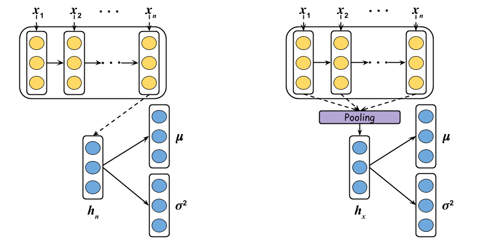
Figure 1: Left: The typical architecture of recognition model for a sequence VAE in which only the last hidden state $h_{n}$ from encoder RNN is used as feature representation to compute the mean $\mu$ and variance $\sigma^{2}$ parameters of approximate posteriors $q_{\phi}(z|x)$. Right: Our proposed modification of how the feature vector $h_{x}$ for sequence $x$ is computed. Specifically, $h_{x}$ is now computed by performing pooling over the temporal dimension of all hidden states $h=[h_{1},h_{2},...,h_{n}]$ output by RNN encoder, which is then used to compute parameters $\mu$ and $\sigma^{2}$ as usual.

4.1 Issues with Last Hidden States

In sequence VAEs, the encoder RNN processes the input sentence $x=[x_{1},x_{2},...,x_{n}]$ one word at a time to produce a series of hidden states $h=[h_{1},h_{2},...,h_{n}]$. In the typical architecture, the last hidden state $h_{n}$ is taken as the feature to compute the mean and variance for the approximate posterior, as shown on the left side of Figure 1, thus:

$$q_{\phi}(z|x)= \mathcal{N}(\mu_{\phi}(x),\sigma_{\phi}^{2}(x))$$

$$\textbf{s.t.}\phantom{\theta}\mu_{\phi}(x) =W_{1}*h_{n}+b_{1}$$

$$\phantom{\theta}\sigma_{\phi}^{2}(x) =\textit{exp}(W_{2}*h_{n}+b_{2})$$

where $W_{1}$, $b_{1}$ and $W_{2}$, $b_{2}$ are the linear layer parameters for mean and log-variance respectively.

However, using the last hidden states as feature representations could be problematic, as RNNs are known to have issues retaining information further back in history. A a result, $h_{n}$ tends to be dominated by later words in the input. We hypothesize that such tendencies of RNNs would result in a feature space with insufficient dispersion.

In the most extreme case, all encoder features would collapse onto a single point regardless of its input, thus there would be no mutual information between the input sequences and their latent variables, which implies $q_{\phi}(z|x)=q_{\phi}(z)$. In practice, features from a space with insufficient dispersion would result in approximate posteriors concentrating in a small region of posterior space, with high chances of overlap for different input data.

As a result, latent codes sampled from different approximate posteriors would look somewhat similar, thus provide little useful information to the decoder. Since no useful information could be conveyed by the latent variables, optimization would push approximate posteriors towards the prior to avoid paying the KL penalty and maximize the overall ELBO objective, thus causing training to reach the undesirable local optimum that is posterior collapse. Therefore we argue that maintaining dispersion of the feature space is important to prevent posterior collapse.

4.2 Increasing Dispersion Reduces Collapse

In order to verify the aforementioned intuition, we train two different sequence VAE models whose encoders are parameterized by LSTMs with only three hidden units and with three-dimensional latent variables on Yahoo dataset Yang et al. (2017). Although it is clearly not the optimal configurations for the encoder and latent variables, doing so would enable us to visualize the feature space produced by the encoders explicitly.

The first model follows standard sequence VAE settings and is trained to optimize the ELBO objective. The other one is trained with an additional Cosine Regularizer that minimizes the pairwise cosine similarities of encoder features within each batch; i.e., $cos(h_{n}^{i},h_{n}^{j})=\frac{h_{n}^{i}\cdot h_{n}^{j}}{\lVert h_{n}^{i}\rVert\lVert h_{n}^{j}\rVert}$ where $h_{n}^{i}$ and $h_{n}^{j}$ are feature vectors for the $i$-th and $j$-th sequences in the batch, in order to examine whether explicitly encouraging feature dispersion would reduce the chance of posterior collapse. Other decorrelation or pairwise repulsion regularizations were explored under different contexts Cogswell et al. (2016); Cao et al. (2018)

Figure 2 a) and b) visualize each feature space on the validation set. Notice that the standard sequence VAE maps all sentences to a concentrated region in feature space. On the other hand, the model trained with the feature cosine regularizer generates more dispersed features. As a result, we can see from Figure 3 that the KL term on validation set quickly converges to close to zero for the vanilla sequence VAE, while the KL term plateaus at non-zero values for model trained with the cosine regularizer. This confirms our intuition that posterior collapse is caused in part by the lack of dispersion in features from the encoder, which in turn result in nearly indistinguishable latent codes for different input sequences.

4.3 Achieving Better Dispersion via Pooling

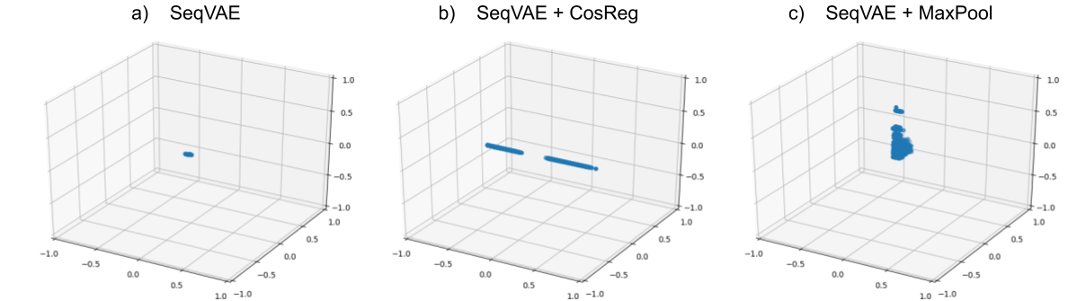
Figure 2: Feature space visualizations on Yahoo validation set for vinilla sequence VAE, sequence VAE with feature cosine regularizer, and sequence VAE with max pooling.

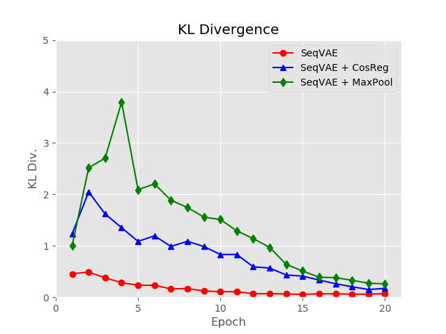
Figure 3: KL diverence on Yahoo validation set (three-dimensional latent variables).

In practice, however, the feature cosine regularizer is not ideal as it can be difficult to optimize for pairwise repulsion objectives in high dimensional space, resuling in inferior model performance. Following our intuition, we want to find better alternatives to generate dispersed features for $x=[x_{1},x_{2},...,x_{n}]$. Ideally, we would want to make use of information across all hidden states instead of just the last step. Thus, we would like the feature vector $h_{x}$ for sequence $x$ to be:

$$h_{x}=\textit{aggregate}([h_{1},h_{2},...,h_{n}])$$

where aggregate is some function that takes a list of vectors and produces a single feature vector.

To avoid adding more parameters to the model, we choose to experiment with different pooling functions. Since attention mechanism is the prevalent method for feature aggregation in many NLP-related tasks, pooling is not as widely used in NLP as in computer vision. However, there have also been successful applications of pooling in NLP, such as multi-task learning Collobert and Weston (2008) and learning pretrained universal sentence encoders Conneau et al. (2017).

In the context of sequence VAE models, we perform pooling over the temporal dimension of hidden states $h=[h_{1},h_{2},...,h_{n}]$ produced by the encoder RNN, as illustrated on the right side of Figure 1. We experiment with three options, the first two are the commonly used average pooling (AvgPool) and max pooling (MaxPool). The last one performs max pooling based on the absolute values of each element while preserving the signs of the pooled elements, which we refer to as sign-preserved absolute pooling (AbsPool).

There are also other alternatives for the aggregate function. One option is to jointly learn a self-attention module to perform the aggregation Yang et al. (2016). We experimented with this approach and found it to be outperformed by pooling-based methods. We suspect that it could be due to the fact that the attention module adds additional parameters to the model and causes it to overfit more easily, thus creating more complications to the already challenging optimization problem.

To examine the effect of pooling on the encoder features, we follow the setup in Section 4.2 and train another model of the same size equipped with max pooling. As shown in Figure 2 c), pooling is able to increase the dispersion in the feature space even more compared to the cosine regularizer. As a result, we can see that the KL term plateaus at higher values in Figure 3, which again aligns with our claim that having dispersed features is causually related to avoiding posterior collapse.

5 Experiments

In this section, we present the main experimental results on benchmark datasets. We also run additional experiments in order to gain more insights into different methods.

5.1 Settings

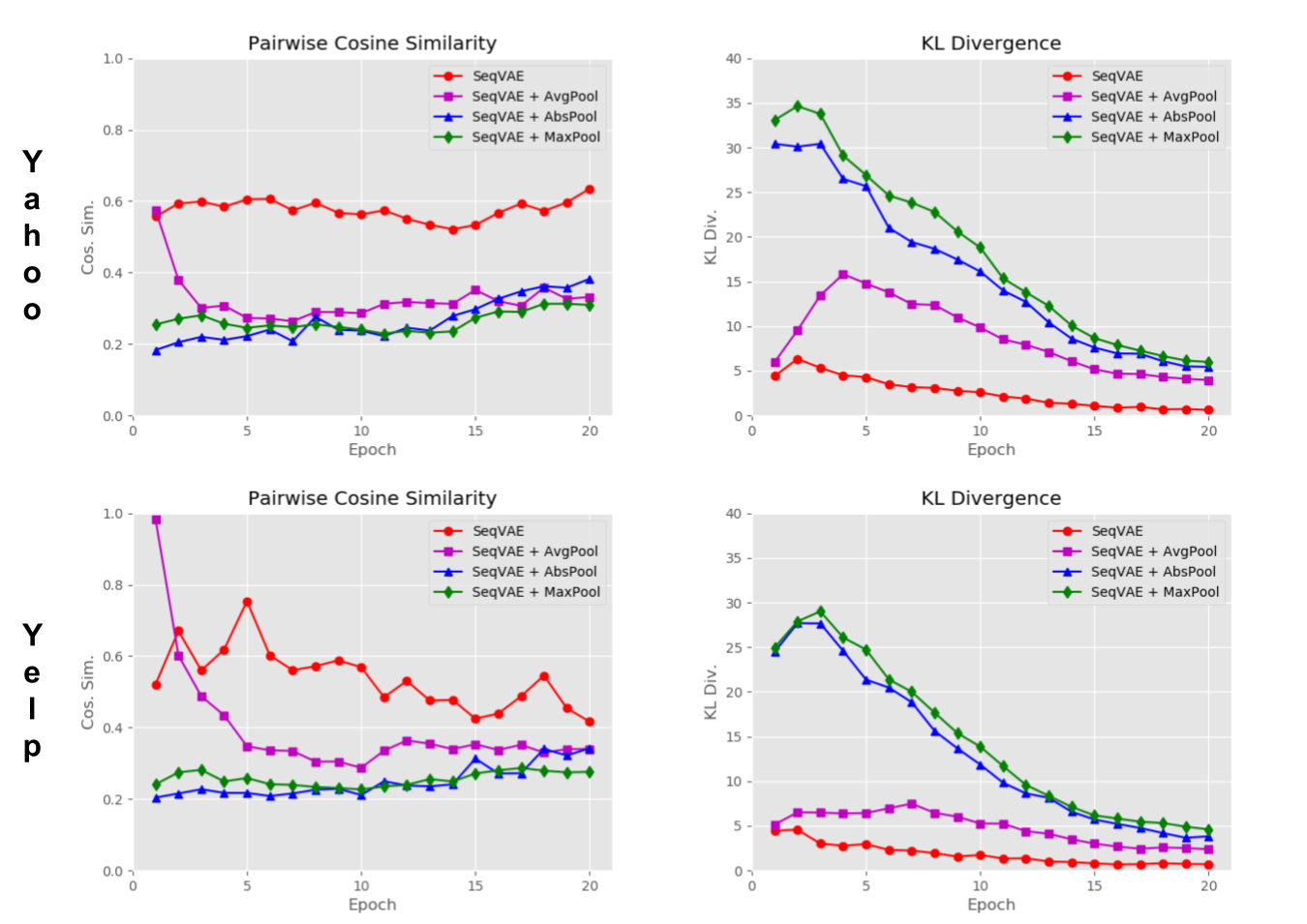
Figure 4: Pairwise cosine similarities between feature vectors and KL divergences for the validation sets. Notice that for regular SeqVAE models, the cosine similarities among different sequences remain at a higher level as the training progresses. At a result, the KL term quickly collapses to close to zero. On the other hand, pooling is able to maintain the dispersion in the feature space, thus helping to avoid posterior collapse.

We evaluate all models on two benchmark datasets for text VAEs: Yahoo and Yelp Yang et al. (2017). Both datasets consist of train, valid, and test splits of 100k, 10k, and 10k sentences, with the average lengths of 78.76 for Yahoo and 96.01 for Yelp.

Following the experiment settings from previous work Kim et al. (2018); He et al. (2019), we employ single-layer LSTMs with 1024 hidden units for both the encoder and decoder with a latent space of 32 dimensions. For all models, we use the isotropic Gaussian $\mathcal{N}(\textbf{0},\textbf{I})$ as prior and the recognition model parameterizes a multivariate Gaussian with diagonal covariance matrix. We train the model standard SGD with early stopping.

5.2 Analysis of Feature Dispersion

For larger models, since we are unable to visualize high dimensional space without losing information, we monitor the pairwise cosine similarities of feature vectors for sequences from the validation set. Figure 4 shows the average pairwise cosine similarities and average KL divergence for both benchmark datasets during training.

Observe that for the regular sequence VAE, the average pairwise cosine similarities on the validation set remain at a higher level compared to the pooling-based models. As the training progresses, KL divergence is quickly pushed to take on small values by the optimization and gradually approach zero, signalling the occurrence of posterior collapse. Whereas for models equipped with pooling, the cosine similarities are kept at a lower level, indicating more dispersed and diverse feature space. As a result, KL terms for pooling-based models converge to non-zero values.

5.3 Quantitative Results

3
	Yahoo					Yelp
Model	NLL	$\overline{\textbf{NLL}}$	KL	MI	AU	NLL	$\overline{\textbf{NLL}}$	KL	MI	AU
3
LSTM-LM*	328.0	–	–	–	–	358.1	–	–	–	–
SeqVAE	328.6	–	0.0	0.0	0	358.1	–	0.3	0.3	1
SeqVAE + WordDrop	330.7	–	5.4	3.0	6	362.2	–	1.0	0.8	1
SkipVAE	328.1	–	4.5	2.4	11	357.4	–	2.5	1.5	4
WAE-RNF**	339.0	–	3.0	–	–	–	–	–	–	–
SeqVAE + Cyclical	328.6	–	0.0	0.0	0	358.4	–	0.4	0.3	1
SeqVAE + Aggressive	326.7	–	5.7	2.9	15	355.9	–	3.8	2.4	11
2
SeqVAE + AvgPool	327.8	–	2.4	1.6	5	357.5	–	1.6	1.2	5
SeqVAE + AbsPool	327.4	–	3.6	2.4	8	356.6	–	2.0	1.7	7
SeqVAE + MaxPool	327.2	–	3.7	2.5	9	356.0	–	3.1	2.2	8
2
iVAE	–	309.5	8.0	4.4	32	–	348.2	7.6	4.6	32
3

Table 1: Experiment results on the Yahoo and Yelp datasets. For the LSTM-LM*, we report the exact negative log likelihood. For the WAE-RNF**, we only show the results on Yahoo reported by Wang and Wang (2019) as their experiments on Yelp were conducted on a different version of the dataset. Note that the estimated negative log likelihood from iVAE (Fang et al., 2019) cannot be directly compared with other methods.

3
	Yahoo	Yelp
	Updates	Updates
3
SeqVAE + Aggressive	608k	625k
SeqVAE + MaxPool	199k	196k
3

Table 2: Computation costs of aggressive training vs max pooling, measured in terms of parameter updates.

We also compare quantitatively with other existing methods on the benchmark datasets. We report approximate negative log likelihood (NLL) estimated by 500 importance weighted samples Burda et al. (2016). We also report KL divergence $D_{KL}(q_{\phi}(z|x)|p(z))$ (KL), estimated mutual information (MI) between $x$ and $z$ Dieng et al. (2019), and number of active units (AU) in the latent codes Burda et al. (2016).

Note that although metrics such as KL, MI, and AU provide certain insights for the models; i.e., whether posterior collapse has occurred for a particular model, they do not directly correlate with the overall qualitiy of a model. Thus higher KL divergence or numbers of active units are not necessarily better, as illustrated by our results. Ultimately, what we want from a model is lower negative log likelihood (with non-zero KL divergence) since it is a direct indicator of how well our models capture the data distribution.

We compare our models with the following methods from the literature: SkipVAE Dieng et al. (2019), WAE-RNF Wang and Wang (2019) which make modifications to decoders or variational distributions; and Cyclical Annealing Liu et al. (2019), Aggressive Training He et al. (2019) which aim to prevent posterior collapse with new optimization schemes. Aggressive training in particular comes with very high computation costs since it requires to train the encoder to near convergence before each decoder update. Additionally, we train two baseline sequence VAE models: one only with KL annealing; and the other with both KL annealing and Word Dropout as in Bowman et al. (2016). All models, including different models from the literature, are trained following a simple linear KL annealing schedule at early stage of training except for ones trained with cyclical annealing schedule.

Fang et al. (2019) proposed to use implicit distributions as the approximate posteriors, for which they named their model implicit VAE (iVAE). At the first glance, their model improved upon the previous methods by a large margin. Howerver, their claimed results $\overline{\textbf{NLL}}$ are in fact a lower bound on the true NLL of the data and thus cannot be directly compared to the results of other models (see Section A in the appendix for more details).

Table 1 shows the quantitative results. We observe that pooling can effectively prevent posterior collapse while achieving significantly lower estimated NLLs compared to standard sequence VAEs, with max pooling offering the best performances on both datasets. This suggests that increasing feature dispersion can effectively prevent posterior collapse, which leads to better overall modelling qualitiy. Applying heavy word dropout leads to non-zero KL term but also worse log likelihood. This indicates that solving posterior collapse is necessary but not sufficient to improve NLLs in sequence VAE models.

Notice that although average pooling also improves upon the baseline model, it provide the least amount of improvements compared to the other two pooling methods. The performance gap is noticeably more significant on Yelp dataset where the average sequence length is longer, which aligns with our intuition that average pooling is likely to produce less dispersion over longer input sequences due to the central limit theorem.

We also see that our methods outperform both SkipVAE and WAE-RNF, which suggests that certain proposed architectural changes might not be necessary to improve upon the original sequence VAE models with Gaussian distributions. Liu et al. (2019) reported promising results for text modelling on the relatively simple Penn Tree Bank (PTB) dataset with their proposed cyclical annealing schedule. However the same success is not carried over to more complex data. Aggressive training gives the best estimated NLLs on both datasets; our methods are able to achieve comparable performances, particularly on the more challenging Yelp dataset where the average length is longer, while being significantly more computationally efficient, as shown in Table 2.

5.4 Comparison with Aggressive Training

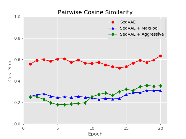
Figure 5: Pairwise cosine similarities between feature vectors on the validation set on Yahoo.

From Table 1, we see that pooling and aggressive training are able to offer much bigger improvements to the standard sequence VAE models compared to other baseline models. To better understand the connections between these two methods, we again monitor the pairwise cosine similarities averaged over the validation set as the training progresses, which is illustrated in Figure 5.

We observe that for both aggressive training and max pooling, the average pairwise cosine similarities among feature representations produced by the encoder are kept at a lower level as opposed to the baseline model, which suggests that the success of aggressive training could also be attributed to the increase of dispersion in feature space. The difference is that aggressive training achieves this with a new optimization scheme whose computation cost is three times higher than our methods. This further support our claim that posterior collapse in sequence VAEs is caused in part by the lack of dispersion in feature space, and increasing dispersion could prevent it from happening.

5.5 How Important is KL Annealing?

3
	Yahoo		Yelp
	W.O.	With	W.O.	With
3
SkipVAE	329.1	328.1	358.2	357.4
Aggressive	328.2	326.7	356.9	355.9
MaxPool	328.6	327.2	357.6	356.0
3

Table 3: Estimated NLLs of various models when trained without vs with KL annealing.

As mentioned previously, the experimental results of various models presented in Section 5.3 were achieved with KL annealing, which is necessary to achieve the best possible data log likelihood. As a matter of fact, it is often used together with the proposed algorithms in order to achieve the best possible results. To illustrate the importance of KL annealing, we compare the estimated NLLs of SkipVAE, Aggressive Training, and MaxPool when trained without and with KL annealing.

As shown in Table 3, KL annealing is indeed rather important and necessary if we want a model that better captures the data distribution. Note that in most cases, the gap for estimated NLLs between whether using it or not is rather significant, suggesting that KL annealing might be able to help the model to better explore during early stage of learning and eventually reach better local optimum. Additional research is needed to better understand the effects of KL annealing in optimizing variational models and why it is so crucial for reaching a better local optimum of ELBO.

6 Conclusion

In this paper, we analyze posterior collapse in sequence VAEs from the perspective of the encoder network. We argue that the issue is caused in part by the lack of dispersion in features from the encoder. We provide empirical evidence to verify this hypothesis and propose a simple architectural change that utilizes pooling operations. Our proposed methods can effectively prevent posterior collapse while achieving comparable or better NLLs compared to existing methods without any additional computation costs.

References

- Alemi et al. (2018) Alexander Alemi, Ben Poole, Ian Fischer, Joshua Dillon, Rif A Saurous, and Kevin Murphy. 2018. Fixing a broken elbo. In International Conference on Machine Learning, pages 159–168.
- Bowman et al. (2016) Samuel R Bowman, Luke Vilnis, Oriol Vinyals, Andrew Dai, Rafal Jozefowicz, and Samy Bengio. 2016. Generating sentences from a continuous space. In Proceedings of The 20th SIGNLL Conference on Computational Natural Language Learning, pages 10–21.
- Burda et al. (2016) Yuri Burda, Roger Grosse, and Ruslan Salakhutdinov. 2016. Importance weighted autoencoders. In International Conference on Learning Representations.
- Cao et al. (2018) Yanshuai Cao, Gavin Weiguang Ding, Kry Yik-Chau Lui, and Ruitong Huang. 2018. Improving gan training via binarized representation entropy (bre) regularization. In International Conference on Learning Representations.
- Cogswell et al. (2016) Michael Cogswell, Faruk Ahmed, Ross Girshick, Larry Zitnick, and Dhruv Batra. 2016. Reducing overfitting in deep networks by decorrelating representations. In International Conference on Learning Representations.
- Collobert and Weston (2008) Ronan Collobert and Jason Weston. 2008. A unified architecture for natural language processing: Deep neural networks with multitask learning. In Proceedings of the 25th international conference on Machine learning, pages 160–167. ACM.
- Conneau et al. (2017) Alexis Conneau, Douwe Kiela, Holger Schwenk, Loïc Barrault, and Antoine Bordes. 2017. Supervised learning of universal sentence representations from natural language inference data. In Proceedings of the 2017 Conference on Empirical Methods in Natural Language Processing, pages 670–680.
- Dieng et al. (2019) Adji B Dieng, Yoon Kim, Alexander M Rush, and David M Blei. 2019. Avoiding latent variable collapse with generative skip models. In Proceedings of the 22nd International Conference on Artificial Intelligence and Statistics (AISTATS 2019).
- Fang et al. (2019) Le Fang, Chunyuan Li, Jianfeng Gao, Wen Dong, and Changyou Chen. 2019. Implicit deep latent variable models for text generation. In EMNLP.
- He et al. (2019) Junxian He, Daniel Spokoyny, Graham Neubig, and Taylor Berg-Kirkpatrick. 2019. Lagging inference networks and posterior collapse in variational autoencoders. In International Conference on Learning Representations.
- Higgins et al. (2017) Irina Higgins, Loic Matthey, Arka Pal, Christopher Burgess, Xavier Glorot, Matthew Botvinick, Shakir Mohamed, and Alexander Lerchner. 2017. beta-vae: Learning basic visual concepts with a constrained variational framework. In International Conference on Learning Representations, volume 3.
- Hu et al. (2017) Zhiting Hu, Zichao Yang, Xiaodan Liang, Ruslan Salakhutdinov, and Eric P Xing. 2017. Toward controlled generation of text. In Proceedings of the 34th International Conference on Machine Learning-Volume 70, pages 1587–1596. JMLR. org.
- Kim et al. (2018) Yoon Kim, Sam Wiseman, Andrew Miller, David Sontag, and Alexander Rush. 2018. Semi-amortized variational autoencoders. In International Conference on Machine Learning, pages 2683–2692.
- Kingma and Welling (2014) Diederik P Kingma and Max Welling. 2014. Auto-encoding variational bayes. In Proceedings of the 2nd International Conference on Learning Representations (ICLR).
- Liu et al. (2019) Xiaodong Liu, Jianfeng Gao, Asli Celikyilmaz, Lawrence Carin, et al. 2019. Cyclical annealing schedule: A simple approach to mitigating kl vanishing. In Proceedings of the 17th Annual Conference of the North American Chapter of the Association for Computational Linguistics: Human Language Technologies (NAACL-HLT 2019).
- Miao and Blunsom (2016) Yishu Miao and Phil Blunsom. 2016. Language as a latent variable: Discrete generative models for sentence compression. In Proceedings of the 2016 Conference on Empirical Methods in Natural Language Processing, pages 319–328.
- Miao et al. (2016) Yishu Miao, Lei Yu, and Phil Blunsom. 2016. Neural variational inference for text processing. In International conference on machine learning, pages 1727–1736.
- Park et al. (2018) Yookoon Park, Jaemin Cho, and Gunhee Kim. 2018. A hierarchical latent structure for variational conversation modeling. In Proceedings of the 2018 Conference of the North American Chapter of the Association for Computational Linguistics: Human Language Technologies, Volume 1 (Long Papers), pages 1792–1801.
- Razavi et al. (2019) Ali Razavi, Aäron van den Oord, Ben Poole, and Oriol Vinyals. 2019. Preventing posterior collapse with delta-vaes. In International Conference on Learning Representations.
- Semeniuta et al. (2017) Stanislau Semeniuta, Aliaksei Severyn, and Erhardt Barth. 2017. A hybrid convolutional variational autoencoder for text generation. In Proceedings of the 2017 Conference on Empirical Methods in Natural Language Processing, pages 627–637.
- Wang and Wang (2019) Prince Zizhuang Wang and William Yang Wang. 2019. Riemannian normalizing flow on variational wasserstein autoencoder for text modeling. In Proceedings of the 2019 Conference of the North American Chapter of the Association for Computational Linguistics: Human Language Technologies, Volume 1 (Long and Short Papers), pages 284–294.
- Wen et al. (2017) Tsung-Hsien Wen, Yishu Miao, Phil Blunsom, and Steve Young. 2017. Latent intention dialogue models. In Proceedings of the 34th International Conference on Machine Learning-Volume 70, pages 3732–3741. JMLR. org.
- Xu and Durrett (2018) Jiacheng Xu and Greg Durrett. 2018. Spherical latent spaces for stable variational autoencoders. In Proceedings of the 2018 Conference on Empirical Methods in Natural Language Processing, pages 4503–4513.
- Xu et al. (2017) Weidi Xu, Haoze Sun, Chao Deng, and Ying Tan. 2017. Variational autoencoder for semi-supervised text classification. In Thirty-First AAAI Conference on Artificial Intelligence.
- Yang et al. (2017) Zichao Yang, Zhiting Hu, Ruslan Salakhutdinov, and Taylor Berg-Kirkpatrick. 2017. Improved variational autoencoders for text modeling using dilated convolutions. In Proceedings of the 34th International Conference on Machine Learning-Volume 70, pages 3881–3890. JMLR. org.
- Yang et al. (2016) Zichao Yang, Diyi Yang, Chris Dyer, Xiaodong He, Alex Smola, and Eduard Hovy. 2016. Hierarchical attention networks for document classification. In Proceedings of the 2016 Conference of the North American Chapter of the Association for Computational Linguistics: Human Language Technologies, pages 1480–1489.
- Zhao et al. (2017) Tiancheng Zhao, Ran Zhao, and Maxine Eskenazi. 2017. Learning discourse-level diversity for neural dialog models using conditional variational autoencoders. In Proceedings of the 55th Annual Meeting of the Association for Computational Linguistics (Volume 1: Long Papers), pages 654–664.