Multi-Armed Bandits with Correlated Arms

\nameSamarth Gupta \emailsamarthg@andrew.cmu.edu
\addrCarnegie Mellon University
Pittsburgh, PA 15213 \AND\nameShreyas Chaudhari \emailschaudh2@andrew.cmu.edu
\addrCarnegie Mellon University
Pittsburgh, PA 15213 \AND\nameGauri Joshi \emailgaurij@andrew.cmu.edu
\addrCarnegie Mellon University
Pittsburgh, PA 15213 \AND\nameOsman Yağan \emailoyagan@andrew.cmu.edu
\addrCarnegie Mellon University
Pittsburgh, PA 15213
Abstract

We consider a multi-armed bandit framework where the rewards obtained by pulling different arms are correlated. We develop a unified approach to leverage these reward correlations and present fundamental generalizations of classic bandit algorithms to the correlated setting. We present a unified proof technique to analyze the proposed algorithms. Rigorous analysis of C-UCB (the correlated bandit versions of Upper-confidence-bound) reveals that the algorithm end up pulling certain sub-optimal arms, termed as non-competitive, only O(1)O1\mathrm{O}(1) times, as opposed to the O(logT)O𝑇\mathrm{O}(\log T) pulls required by classic bandit algorithms such as UCB, TS etc. We present regret-lower bound and show that when arms are correlated through a latent random source, our algorithms obtain order-optimal regret. We validate the proposed algorithms via experiments on the MovieLens and Goodreads datasets, and show significant improvement over classical bandit algorithms.

1 Introduction

1.1 Background and Motivation

Classical Multi-armed Bandits. The multi-armed bandit (MAB) problem falls under the class of sequential decision making problems. In the classical multi-armed bandit problem, there are K𝐾K arms, with each arm having an unknown reward distribution. At each round t𝑡t, we need to decide an arm kt𝒦subscript𝑘𝑡𝒦k_{t}\in\mathcal{K} and we receive a random reward Rktsubscript𝑅subscript𝑘𝑡R_{k_{t}} drawn from the reward distribution of arm ktsubscript𝑘𝑡k_{t}. The goal in the classical multi-armed bandit is to maximize the long-term cumulative reward. In order to maximize cumulative reward, it is important to balance the exploration-exploitation trade-off, i.e., pulling each arm enough number of times to identify the one with the highest mean reward, while trying to make sure that the arm with the highest mean reward is played as many times as possible. This problem has been well studied starting with the work of Lai and Robbins [1] that proposed the upper confidence bound (UCB) arm-selection algorithm and studied its fundamental limits in terms of bounds on regret. Subsequently, several other algorithms including Thompson Sampling (TS) [2] and KL-UCB [3], have been proposed for this setting. The generality of the classical multi-armed bandit model allows it to be useful in numerous applications. For example, MAB algorithms are useful in medical diagnosis [4], where the arms correspond to the different treatment mechanisms/drugs and are widely used for the problem of ad optimization [5] by viewing different version of ads as the arms in the MAB problem. The MAB framework is also useful in system testing [6], scheduling in computing systems [7, 8, 9], and web optimization [10, 5].

Correlated Multi-Armed Bandits. The classical MAB setting implicitly assumes that the rewards are independent across arms, i.e., pulling an arm k𝑘k does not provide any information about the reward we would have received from arm \ell. However, this may not be true in practice as the reward corresponding to different treatment/drugs/ad-versions are likely to be correlated with each other. For instance, similar ads/drugs may generate similar reward for the user/patient. These correlations, when modeled and accounted for, can allow us to significantly improve the cumulative reward by reducing the amount of exploration in bandit algorithms.
Refer to caption
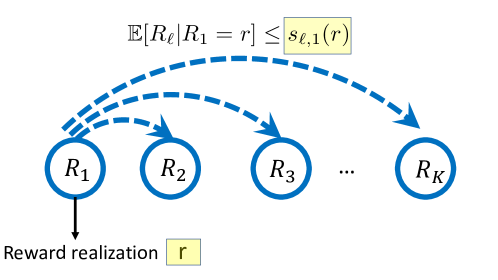
Figure 1: Upon observing a reward r𝑟r from an arm k𝑘k, pseudo-rewards s,k(r),subscript𝑠𝑘𝑟s_{\ell,k}(r), give us an upper bound on the conditional expectation of the reward from arm \ell given that we observed reward r𝑟r from arm k𝑘k. These pseudo-rewards models the correlation in rewards corresponding to different arms.

Motivated by this, we study a variant of the classical multi-armed bandit problem in which rewards corresponding to different arms are correlated to each other, i.e., the conditional reward distribution satisfies fR|Rk(r|rk)fR(r)subscript𝑓conditionalsubscript𝑅subscript𝑅𝑘conditionalsubscript𝑟subscript𝑟𝑘subscript𝑓subscript𝑅subscript𝑟f_{R_{\ell}|R_{k}}(r_{\ell}|r_{k})\neq f_{R_{\ell}}(r_{\ell}), whence 𝔼[R|Rk]𝔼[R]𝔼delimited-[]conditionalsubscript𝑅subscript𝑅𝑘𝔼delimited-[]subscript𝑅\mathbb{E}\left[{R_{\ell}|R_{k}}\right]\neq\mathbb{E}\left[{R_{\ell}}\right]. Such correlations can only be learned upon obtaining samples from different arms simultaneously, i.e., by pulling multiple arms at a time. As that is not allowed in the classical Multi-Armed Bandit formulation, we assume the knowledge of such correlations in the form of prior knowledge that might be obtained through domain expertise or from controlled surveys. One way of capturing correlations is through the knowledge of the joint reward distribution. However, if the complete joint reward distribution is known, then the best-arm is known trivially. Instead, in our work, we only assume restrictive information about correlations in the form of pseudo-rewards that constitute an upper bound on conditional expected rewards. This makes our model more general and suitable for practical applications. Fig. 1 presents an illustration of our model, where the pseudo-rewards, denoted by s,k(r)subscript𝑠𝑘𝑟s_{\ell,k}(r), provide an upper bound on the reward that we could have received from arm \ell given that pulling arm k𝑘k led to a reward of r𝑟r; i.e.,

𝔼[R|Rk=r]s,k(r).𝔼delimited-[]conditionalsubscript𝑅subscript𝑅𝑘𝑟subscript𝑠𝑘𝑟\mathbb{E}[R_{\ell}|R_{k}=r]\leq s_{\ell,k}(r). (1)

We show that the knowledge of such bounds, even when they are not all tight, can lead to significant improvement in the cumulative reward obtained by reducing the amount of exploration compared to classical MAB algorithms. Our proposed MAB model and algorithm can be applied in all real-world applications of the classical Multi-Armed bandit problem, where it is possible to know pseudo-rewards from domain knowledge or through surveyed data. In the next section, we illustrate the applicability of our novel correlated Multi-Armed Bandit model and its differences with the existing contextual and structured bandit works through the example of optimal ad-selection.

1.2 An Illustrative Example

Suppose that a company is to run a display advertising campaign for one of their products, and its creative team have designed several different versions that can be displayed. It is expected that the user engagement (in terms of click probability and time spent looking at the ad) depends the version of the ad that is displayed. In order to maximize the total user engagement over the course of the ad campaign, multi-armed bandit algorithms can be used; different versions of the ad correspond to the arms and the reward from selecting an arm is given by the clicks or time spent looking at the ad version corresponding to that arm.
Refer to caption
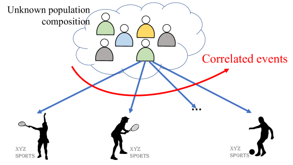
Figure 2: The ratings of a user corresponding to different versions of the same ad are likely to be correlated. For example, if a person likes first version, there is a good chance that they will also like the 2nd one as it also related to tennis. However, the population composition is unknown, i.e., the fraction of people liking the first/second or the last version is unknown.

Personalized recommendations using Contextual and Structured bandits. Although the ad-selection problem can be solved by standard MAB algorithms, there are several specialized MAB variants that are designed to give better performance. For instance, the contextual bandit problem [11, 12] has been studied to provide personalized displays of the ads to the users. Here, before making a choice at each time step (i.e., deciding which version to show to a user), we observe the context associated with that user (e.g., age/occupation/income features). Contextual bandit algorithms learn the mappings from the context θ𝜃\theta to the most favored version of ad k(θ)superscript𝑘𝜃k^{*}(\theta) in an online manner and thus are useful for personalized recommendations. A closely related problem is the structured bandit problem [13, 14, 15, 16], in which the context θ𝜃\theta (age/ income/ occupational features) is hidden but the mean rewards for different versions of ad (arms) as a function of hidden context θ𝜃\theta are known. Such models prove useful for personalized recommendation in which the context of the user is unknown, but the reward mappings μk(θ)subscript𝜇𝑘𝜃\mu_{k}(\theta) are known through surveyed data.

Global Recommendations using Correlated-Reward Bandits. In this work we study a variant of the classical multi-armed bandit problem in which rewards corresponding to different arms are correlated to each other. In many practical settings, the reward we get from different arms at any given step are likely to be correlated. In the ad-selection example given in Figure 2, a user reacting positively (by clicking, ordering, etc.) to the first version of the ad with a girl playing tennis might also be more likely to click the second version as it is also related to tennis; of course one can construct examples where there is negative correlation between click events to different ads. The model we study in this paper explicitly captures these correlations through the knowledge of pseudo-rewards s,k(r)subscript𝑠𝑘𝑟s_{\ell,k}(r) (See Figure 1). Similar to the classical MAB setting, the goal here is to display versions of the ad to maximize user engagement. In addition, unlike contextual bandits, we do not observe the context (age/occupational/income) features of the user and do not focus on providing personalized recommendation. Instead our goal is to provide global recommendations to a population whose demographics is unknown. Unlike structured bandits, we do not assume that the mean rewards are functions of a hidden context parameter θ𝜃\theta. In structured bandits, although the mean rewards depend on θ𝜃\theta the reward realizations can still be independent. See Section 2.4 for more details.

1.3 Main Contributions and Organization

i) A General and Previously Unexplored Correlated Multi-Armed Bandit Model. In Section 2 we describe our novel correlated multi-armed bandit model, in which rewards of a user corresponding to different arms are correlated with each other. This correlation is captured by the knowledge of pseudo-rewards, which are upper bounds on the conditional mean reward of arm \ell given reward of arm k𝑘k. In practice, pseudo-rewards can be obtained via expert/domain knowledge (for example, common ingredients in two drugs that are being considered to treat an ailment) or controlled surveys (for example, beta-testing users who are asked to rate different versions of an ad). A key advantage of our framework is that pseudo-rewards are just upper bounds on the conditional expected rewards and can be arbitrarily loose. This also makes the proposed framework and algorithm directly usable in practice – if some pseudo-rewards are unknown due to lack of domain knowledge/data, they can simply be replaced by the maximum possible reward entries, which serves a natural upper bound.

ii) An approach to generalize algorithms to the Correlated MAB setting. We propose a novel approach in Section 3 that extends any classical bandit (such as UCB, TS, KL-UCB etc.) algorithm to the correlated MAB setting studied in this paper. This is done by making use of the pseudo-rewards to reduce exploration in standard bandit algorithms. We refer to this algorithm as C-Bandit where Bandit refers to the classical bandit algorithm used in the last step of the algorithm (i.e., UCB/TS/KL-UCB).

iii) Unified Regret Analysis We study the performance of our proposed algorithms by analyzing their expected regret, 𝔼[Reg(T)]𝔼delimited-[]Reg𝑇\mathbb{E}\left[{\text{Reg}(T)}\right]. The regret of an algorithm is defined as the difference between the cumulative reward of a genie policy, that always pulls the optimal arm ksuperscript𝑘k^{*}, and the cumulative reward obtained by the algorithm over T𝑇T rounds. By doing regret analysis of C-UCB, we obtain the following upper bound on the expected regret of C-UCB.

Proposition 1 (Upper Bound on Expected Regret).

The expected cumulative regret of the C-UCB algorithm is upper bounded as

𝔼[Reg(T)](C1)O(logT)+O(1),𝔼delimited-[]𝑅𝑒𝑔𝑇𝐶1O𝑇O1\mathbb{E}\left[{Reg(T)}\right]\leq(C-1)\cdot\mathrm{O}(\log T)+\mathrm{O}(1), (2)

Here C𝐶C denotes the number of competitive arms. An arm k𝑘k is said to be competitive if expected pseudo-reward of arm k𝑘k with respect to the optimal arm ksuperscript𝑘k^{*} is larger than the mean reward of arm ksuperscript𝑘k^{*}, that is, if 𝔼[sk,k(r)]μk𝔼delimited-[]subscript𝑠𝑘superscript𝑘𝑟subscript𝜇superscript𝑘\mathbb{E}\left[{s_{k,k^{*}}(r)}\right]\geq\mu_{k^{*}}, otherwise, the arm is said to be non-competitive. The result in 2 arises from the fact that the C-UCB algorithm ends up pulling the non-competitive arms only O(1)O1\mathrm{O}(1) times and only the competitive sub-optimal arms are pulled O(logT)O𝑇\mathrm{O}(\log T) times. In contrast to UCB, that pulls all K1𝐾1K-1 sub-optimal arms O(logT)O𝑇\mathrm{O}(\log T) times, our proposed C-UCB algorithm pulls only C1K1𝐶1𝐾1C-1\leq K-1 arms O(logT)O𝑇\mathrm{O}(\log T) times. In fact, when C=1𝐶1C=1, our proposed algorithm achieves bounded regret meaning that after some finite step, no arm but the optimal one will be selected. In this sense, we reduce a K𝐾K-armed bandit problem to a C𝐶C-armed bandit problem. We emphasize that ksuperscript𝑘k^{*}, μsuperscript𝜇\mu^{*} and C𝐶C are all unknown to the algorithm at the beginning.

We present our detailed regret bounds and analysis in Section 4. A rigorous analysis of the regret achieved under C-UCB is given through a unified technique. This technique can be of broad interest as we also provide a recipe to obtain regret analysis for any C-Bandit algorithm. For instance, the analysis of C-KL-UCB can be easily done through our provided outline.

iv) Evaluation using real-world datasets.

We perform simulations to validate our theoretical results in Section 5. In Section 6, we do extensive validation of our results by performing experiments on two real-world datasets, namely Movielens and Goodreads, which show that the proposed approach yields drastically smaller regret than classical Multi-Armed Bandit strategies.

2 Problem Formulation

2.1 Correlated Multi-Armed Bandit Model

r s2,1(r)subscript𝑠21𝑟s_{2,1}(r) r s1,2(r)subscript𝑠12𝑟s_{1,2}(r)
0 0.7 0 0.8
1 0.4 1 0.5
(a) R1=0subscript𝑅10R_{1}=0 R1=1subscript𝑅11R_{1}=1
R2=0subscript𝑅20R_{2}=0 0.2 0.4
R2=1subscript𝑅21R_{2}=1 0.2 0.2
(b) R1=0subscript𝑅10R_{1}=0 R1=1subscript𝑅11R_{1}=1
R2=0subscript𝑅20R_{2}=0 0.2 0.3
R2=1subscript𝑅21R_{2}=1 0.4 0.1
Table 1: The top row shows the pseudo-rewards of arms 1 and 2, i.e., upper bounds on the conditional expected rewards (which are known to the player). The bottom row depicts two possible joint probability distribution (unknown to the player). Under distribution (a), Arm 1 is optimal whereas Arm 2 is optimal under distribution (b).

Consider a Multi-Armed Bandit setting with K𝐾K arms {1,2,K}12𝐾\{1,2,\ldots K\}. At each round t𝑡t, a user enters the system and we need to decide an arm ktsubscript𝑘𝑡k_{t} to display to the user. Upon pulling arm ktsubscript𝑘𝑡k_{t}, we receive a random reward Rkt[0,B]subscript𝑅subscript𝑘𝑡0𝐵R_{k_{t}}\in[0,B]. Our goal is to maximize the cumulative reward over time. The expected reward of arm k𝑘k, is denoted by μksubscript𝜇𝑘\mu_{k}. If we knew the arm with highest mean, i.e., k=argmaxk𝒦μksuperscript𝑘subscript𝑘𝒦subscript𝜇𝑘k^{*}=\arg\max_{k\in\mathcal{K}}\mu_{k} beforehand, then we would always pull arm ksuperscript𝑘k^{*} to maximize expected cumulative reward. We now define the cumulative regret, minimizing which is equivalent to maximizing cumulative reward:

Reg(T)=t=1Tμktμk=kknk(T)Δk.𝑅𝑒𝑔𝑇superscriptsubscript𝑡1𝑇subscript𝜇subscript𝑘𝑡subscript𝜇superscript𝑘subscript𝑘superscript𝑘subscript𝑛𝑘𝑇subscriptΔ𝑘Reg(T)=\sum_{t=1}^{T}\mu_{k_{t}}-\mu_{k^{*}}=\sum_{k\neq k^{*}}n_{k}(T)\Delta_{k}. (3)

Here, nk(T)subscript𝑛𝑘𝑇n_{k}(T) denotes the number of times a sub-optimal arm is pulled till round T𝑇T and ΔksubscriptΔ𝑘\Delta_{k} denotes the sub-optimality gap of arm k𝑘k, i.e., Δk=μkμksubscriptΔ𝑘subscript𝜇superscript𝑘subscript𝜇𝑘\Delta_{k}=\mu_{k^{*}}-\mu_{k}.

The classical multi-Armed bandit setting implicitly assumes the rewards R1,R2RKsubscript𝑅1subscript𝑅2subscript𝑅𝐾R_{1},R_{2}\ldots R_{K} are independent, that is, Pr(R=r|Rk=r)=Pr(R=r)r,r&,k,Prsubscript𝑅conditionalsubscript𝑟subscript𝑅𝑘𝑟Prsubscript𝑅subscript𝑟for-allsubscript𝑟𝑟for-all𝑘\Pr(R_{\ell}=r_{\ell}|R_{k}=r)=\Pr(R_{\ell}=r_{\ell})\quad\forall{r_{\ell},r}\&\forall{\ell,k}, which implies that, 𝔼[R|Rk=r]=𝔼[R]r,,k𝔼delimited-[]conditionalsubscript𝑅subscript𝑅𝑘𝑟𝔼delimited-[]subscript𝑅for-all𝑟𝑘\mathbb{E}\left[{R_{\ell}|R_{k}=r}\right]=\mathbb{E}\left[{R_{\ell}}\right]\quad\forall{r,\ell,k}. However, in most practical scenarios this assumption is unlikely to be true. In fact, rewards of a user corresponding to different arms are likely to be correlated. Motivated by this we consider a setup where the conditional distribution of the reward from arm \ell given reward from arm k𝑘k is not equal to the probability distribution of the reward from arm \ell, i.e., fR|Rk(r|rk)fR(r)subscript𝑓conditionalsubscript𝑅subscript𝑅𝑘conditionalsubscript𝑟subscript𝑟𝑘subscript𝑓subscript𝑅subscript𝑟f_{R_{\ell}|R_{k}}(r_{\ell}|r_{k})\neq f_{R_{\ell}}(r_{\ell}), with fR(r)subscript𝑓subscript𝑅subscript𝑟f_{R_{\ell}}(r_{\ell}) denoting the probability distribution function of the reward from arm \ell. Consequently, due to such correlations, we have 𝔼[R|Rk]𝔼[R]𝔼delimited-[]conditionalsubscript𝑅subscript𝑅𝑘𝔼delimited-[]subscript𝑅\mathbb{E}\left[{R_{\ell}|R_{k}}\right]\neq\mathbb{E}\left[{R_{\ell}}\right].

In our problem setting, we consider that the player has partial knowledge about the joint distribution of correlated arms in the form of pseudo-rewards, as defined below:

Definition 1 (Pseudo-Reward).

Suppose we pull arm k𝑘k and observe reward r𝑟r, then the pseudo-reward of arm \ell with respect to arm k𝑘k, denoted by s,k(r)subscript𝑠𝑘𝑟s_{\ell,k}(r), is an upper bound on the conditional expected reward of arm \ell, i.e.,

𝔼[R|Rk=r]s,k(r),𝔼delimited-[]conditionalsubscript𝑅subscript𝑅𝑘𝑟subscript𝑠𝑘𝑟\mathbb{E}[R_{\ell}|R_{k}=r]\leq s_{\ell,k}(r), (4)

without loss of generality, we define s,(r)=rsubscript𝑠𝑟𝑟s_{\ell,\ell}(r)=r.

The pseudo-rewards information consists of a set of K×K𝐾𝐾K\times K functions s,k(r)subscript𝑠𝑘𝑟s_{\ell,k}(r) over [0,B]0𝐵[0,B]. This information can be obtained in practice through either domain/expert knowledge or from controlled surveys. For instance, in the context of medical testing, where the goal is to identify the best drug to treat an ailment from among a set of K𝐾K possible options, the effectiveness of two drugs is correlated when the drugs share some common ingredients. Through domain knowledge of doctors, it is possible answer questions such as “what are the chances that drug B𝐵B would be effective given drug A𝐴A was not effective?", through which we can infer the pseudo-rewards.

r s2,1(r)subscript𝑠21𝑟s_{2,1}(r) s3,1(r)subscript𝑠31𝑟s_{3,1}(r)
0 0.7 2
1 0.8 1.2
2 2 1
r s1,2(r)subscript𝑠12𝑟s_{1,2}(r) s3,2(r)subscript𝑠32𝑟s_{3,2}(r)
0 0.5 1.5
1 1.3 2
2 2 0.8
r s1,3(r)subscript𝑠13𝑟s_{1,3}(r) s2,3(r)subscript𝑠23𝑟s_{2,3}(r)
0 1.5 2
1 2 1.3
2 0.7 0.75
Table 2: If some pseudo-reward entries are unknown (due to lack of prior-knowledge/data), those entries can be replaced with the maximum possible reward and then used in the C-BANDIT algorithm. We do that here by entering 222 for the entries where pseudo-rewards are unknown.

2.2 Computing Pseudo-Rewards from prior-data/surveys

The pseudo-rewards can also be learned from prior-available data, or through offline surveys in which users are presented with all K𝐾K arms allowing us to sample R1,,RKsubscript𝑅1subscript𝑅𝐾R_{1},\ldots,R_{K} jointly. Through such data, we can evaluate an estimate on the conditional expected rewards. For example in Table 1, we can look at all users who obtained 00 reward for Arm 1 and calculate their average reward for Arm 2, say μ^2,1(0)subscript^𝜇210\hat{\mu}_{2,1}(0). This average provides an estimate on the conditional expected reward. Since we only need an upper bound on 𝔼[R2|R1=0]𝔼delimited-[]conditionalsubscript𝑅2subscript𝑅10\mathbb{E}\left[{R_{2}|R_{1}=0}\right], we can use several approaches to construct the pseudo-rewards.

  1. 1.

    If the training data is large, one can use the empirical estimate μ^2,1(0)subscript^𝜇210\hat{\mu}_{2,1}(0) directly as s2,1(0)subscript𝑠210s_{2,1}(0), because through law of large numbers, the empirical average equals the 𝔼[R2|R1=0]𝔼delimited-[]conditionalsubscript𝑅2subscript𝑅10\mathbb{E}\left[{R_{2}|R_{1}=0}\right].

  2. 2.

    Alternatively, we can set s2,1(0)=μ^2,1(0)+σ^2,1(0)subscript𝑠210subscript^𝜇210subscript^𝜎210s_{2,1}(0)=\hat{\mu}_{2,1}(0)+\hat{\sigma}_{2,1}(0), with σ^2,1(0)subscript^𝜎210\hat{\sigma}_{2,1}(0) denoting the empirical standard deviation on the conditional reward of arm 2, to ensure that pseudo-reward is an upper bound on the conditional expected reward.

  3. 3.

    In addition, pseudo-rewards for any unknown conditional mean reward could be filled with the maximum possible reward for the corresponding arm. Table 2 shows an example of a 3-armed bandit problem where some pseudo-reward entries are unknown, e.g., due to lack of data. We can fill these missing entries with maximum possible reward (i.e.,2)(i.e.,2) as shown in Table 2 to complete the pseudo-reward entries.

  4. 4.

    If through the training data, we obtain a soft upper bound u𝑢u on 𝔼[R2|R1=0]𝔼delimited-[]conditionalsubscript𝑅2subscript𝑅10\mathbb{E}\left[{R_{2}|R_{1}=0}\right] that holds with probability 1δ1𝛿1-\delta, then we can translate it to the pseudo-reward s2,1(0)=u×(1δ)+2×δsubscript𝑠210𝑢1𝛿2𝛿s_{2,1}(0)=u\times(1-\delta)+2\times\delta, (assuming maximum possible reward is 2).

Remark 1.

Note that the pseudo-rewards are upper bounds on the expected conditional reward and not hard bounds on the conditional reward itself. This makes our problem setup practical as upper bounds on expected conditional reward are easier to obtain, as illustrated in the previous paragraph.

Remark 2 (Reduction to Classical Multi-Armed Bandits).

When all pseudo-reward entries are unknown, then all pseudo-reward entries can be filled with maximum possible reward for each arm, that is, s,k(r)=Bsubscript𝑠𝑘𝑟𝐵s_{\ell,k}(r)=B r,,kfor-all𝑟𝑘\forall{r,\ell,k}. In such a case, the problem framework studied in this paper reduces to the setting of the classical Multi-Armed Bandit problem and our proposed C-Bandit algorithm performs exactly as standard bandit (for e.g., UCB, TS etc.) algorithms.

While the pseudo-rewards are known in our setup, the underlying joint probability distribution of rewards is unknown. For instance, Table 1 (a) and Table 1 (b) show two joint probability distributions of the rewards that are both possible given the pseudo-rewards at the top of Table 1. If the joint distribution is as given in Table 1 (a), then Arm 1 is optimal, while Arm 2 is optimal if the joint distribution is as given in Table 1(b).

Remark 3.

For a setting where reward domain is large or there are a large number of arms, it may be difficult to learn the pseudo-reward entries from prior-data. In such scenarios, the knowledge of additional correlation structure may be helpful to know the value of pseudo-rewards. We describe one such structure in the next section where rewards are correlated through a latent random source and show how to evaluate pseudo-rewards in such a scenario.

2.3 Special Case: Correlated Bandits with a Latent Random Source
Refer to caption
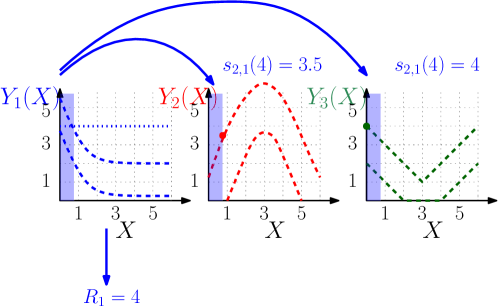
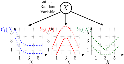
Figure 3: A special case of our proposed problem framework is a setting in which rewards for different arms are correlated through a hidden random variable X. At each round X𝑋X takes a realization in 𝒳𝒳\mathcal{X}. The reward obtained from an arm k𝑘k is Yk(X)subscript𝑌𝑘𝑋Y_{k}(X). The figure illustrates lower bounds and upper bounds on Yk(X)subscript𝑌𝑘𝑋Y_{k}(X) (through dotted lines). For instance, when X𝑋X takes the realization 111, reward of arm 3 is a random variable bounded between 111 and 333.
Refer to caption
Figure 4: An illustration on how to calculate pseudo-rewards in CMAB with latent random source. Upon observing a reward of 4 from arm 1, we can see that the maximum possible reward for arms 2 and 3 is 3.5 and 4 respectively. Therefore, s2,1(4)=3.5subscript𝑠2143.5s_{2,1}(4)=3.5 and s3,1(4)=4subscript𝑠3144s_{3,1}(4)=4.

Our proposed correlated multi-armed bandit framework subsumes many interesting and previously unexplored multi-armed bandit settings. One such special case is the correlated multi-armed bandit model where the rewards depend on a common latent source of randomness [17]. More concretely, the rewards of different arms are correlated through a hidden random variable X𝑋X (see Figure 3). At each round t𝑡t, X𝑋X takes a an i.i.d. realization Xt𝒳subscript𝑋𝑡𝒳X_{t}\in\mathcal{X} (unobserved to the player) and upon pulling arm k𝑘k, we observe a random reward Yk(Xt)subscript𝑌𝑘subscript𝑋𝑡Y_{k}(X_{t}). The latent random variable X𝑋X here could represent the features (i.e., age/occupation etc.) of the user arriving to the system, to whom we show one of the K𝐾K arms. These features of the user are hidden in the problem due to privacy concerns. The random reward Yk(Xt)subscript𝑌𝑘subscript𝑋𝑡Y_{k}(X_{t}) represents the preference of user with context Xtsubscript𝑋𝑡X_{t} for the kthsuperscript𝑘𝑡k^{th} version of the ad, for the application of ad-selection.

In this problem setup, upper and lower bounds on Yk(X)subscript𝑌𝑘𝑋Y_{k}(X), namely g¯k(X)subscript¯𝑔𝑘𝑋\bar{g}_{k}(X) and g¯k(X)subscript¯𝑔𝑘𝑋\underline{g}_{k}(X) are known. For instance, the information on upper and lower bounds of Yk(Xt)subscript𝑌𝑘subscript𝑋𝑡Y_{k}(X_{t}) could represent knowledge of the form that children of age 5-10 rate documentaries only in the range 1-3 out of 5. Such information can be known or learned through prior available data. While the bounds on Yk(X)subscript𝑌𝑘𝑋Y_{k}(X) are known, the distribution of X𝑋X and reward distribution within the bounds is unknown, due to which the optimal arm is not known beforehand. Thus, an online approach is needed to minimize the regret.

It is possible to translate this setting to the general framework described in the problem by transforming the mappings Yk(X)subscript𝑌𝑘𝑋Y_{k}(X) to pseudo-rewards s,k(r)subscript𝑠𝑘𝑟s_{\ell,k}(r). Recall the pseudo-rewards represent an upper bound on the conditional expectation of the rewards. In this framework, s,k(r)subscript𝑠𝑘𝑟s_{\ell,k}(r) can be calculated as:

s,k(r)=max{x:g¯k(x)rg¯k(x)}g¯(x),subscript𝑠𝑘𝑟subscriptconditional-set𝑥subscript¯𝑔𝑘𝑥𝑟subscript¯𝑔𝑘𝑥subscript¯𝑔𝑥s_{\ell,k}(r)=\max_{\{x:\underline{g}_{k}(x)\leq r\leq\bar{g}_{k}(x)\}}\bar{g}_{\ell}(x),

where g¯k(x)subscript¯𝑔𝑘𝑥\underline{g}_{k}(x) and g¯k(x)subscript¯𝑔𝑘𝑥\bar{g}_{k}(x) represent upper and lower bounds on Yk(x)subscript𝑌𝑘𝑥Y_{k}(x). Upon observing a realization from arm k𝑘k, it is possible to estimate the maximum possible reward that would have been obtained from arm \ell through the knowledge of bounds on Yk(X)subscript𝑌𝑘𝑋Y_{k}(X).

Figure 4 illustrates how pseudo-reward is evaluated when we obtain a reward r=4𝑟4r=4 by pulling arm 1. We first infer that X𝑋X lies in [0,0.8]00.8[0,0.8] if r=4𝑟4r=4 and then find the maximum possible reward for arm 2 and arm 3 in [0,0.8]00.8[0,0.8]. Once these pseudo-rewards are constructed, the problem fits in the general framework described in this paper and we can use the algorithms proposed for this setting directly.

Remark 4.

In the scenario where g¯k(x)subscript¯𝑔𝑘𝑥\underline{g}_{k}(x) and g¯k(x)subscript¯𝑔𝑘𝑥\bar{g}_{k}(x) are soft lower and upper bounds, i.e., g¯k(x)Yk(x)g¯k(x)subscript¯𝑔𝑘𝑥subscript𝑌𝑘𝑥subscript¯𝑔𝑘𝑥\underline{g}_{k}(x)\leq Y_{k}(x)\leq\bar{g}_{k}(x) w.p. 1δ1𝛿1-\delta, we can still construct pseudo-reward as follows:

s,k(r)=(1δ)2×(max{x:g¯k(x)rg¯k(x)}g¯(x))+(1(1δ)2)×M,subscript𝑠𝑘𝑟superscript1𝛿2subscriptconditional-set𝑥subscript¯𝑔𝑘𝑥𝑟subscript¯𝑔𝑘𝑥subscript¯𝑔𝑥1superscript1𝛿2𝑀s_{\ell,k}(r)=(1-\delta)^{2}\times\left(\max_{\{x:\underline{g}_{k}(x)\leq r\leq\bar{g}_{k}(x)\}}\bar{g}_{\ell}(x)\right)+(1-(1-\delta)^{2})\times M,

where M𝑀M is the maximum possible reward an arm can provide. Thus our proposed framework and algorithms work under this setting as well.111We evaluate a range of values within which x𝑥x lies based on the reward with probability 1δ1𝛿1-\delta. The maximum possible reward of arm \ell for values of x𝑥x is then identified with probability 1δ1𝛿1-\delta. Due to this, with probability (1δ)2superscript1𝛿2(1-\delta)^{2}, conditional reward of arm \ell is at-most max{x:g¯k(x)rg¯k(x)}g¯(x)subscriptconditional-set𝑥subscript¯𝑔𝑘𝑥𝑟subscript¯𝑔𝑘𝑥subscript¯𝑔𝑥\max_{\{x:\underline{g}_{k}(x)\leq r\leq\bar{g}_{k}(x)\}}\bar{g}_{\ell}(x).

2.4 Comparison with parametric (structured) models

As mentioned in Section 1, a seemingly related model is the structured bandits model [13, 14, 18]. Structured bandits is a class of problems that cover linear bandits [15], generalized linear bandits [19], Lipschitz bandits [20], global bandits [21], regional bandits [22] etc. In the structured bandits setup, mean rewards corresponding to different arms are related to one another through a hidden parameter θ𝜃\theta. The underlying value of θ𝜃\theta is fixed and the mean reward mappings θμk(θ)𝜃subscript𝜇𝑘𝜃\theta\rightarrow\mu_{k}(\theta) are known. Similarly, [23] studies a dependent armed bandit problem, that also has mean rewards corresponding to different arms related to one another. It considers a parametric model, where mean rewards of different arms are drawn from one of the K𝐾K clusters, each having an unknown parameter πisubscript𝜋𝑖\pi_{i}. All of these models are fundamentally different from the problem setting considered in this paper. We list some of the differences with the structured bandits (and the model in [23]) below.

  1. 1.

    In this work we explicitly model the correlations in the rewards of a user corresponding to different arms. While mean rewards are related to each other in structured bandits and [23], the reward realizations are not necessarily correlated.

  2. 2.

    The model studied here is non-parametric in the sense that there is no hidden feature space as is the case in structured bandits and the work of Pandey et al. [23].

  3. 3.

    In structured bandits, the reward mappings from θ𝜃\theta to μk(θ)subscript𝜇𝑘𝜃\mu_{k}(\theta) need to be exact. If they happen to be incorrect, then the algorithms for structured bandit cannot be used as they rely on the correctness of μk(θ)subscript𝜇𝑘𝜃\mu_{k}(\theta) to construct confidence intervals on the unknown parameter θ𝜃\theta. In contrast, the model studied here relies on the pseudo-rewards being upper bounds on conditional expectations. These bounds need not be tight and the proposed C-Bandit algorithms adjust accordingly and perform at least as well as the corresponding classical bandit algorithm.

  4. 4.

    Similar to the structured bandits, the unimodal bandit framework [24, 25] also assumes a structure on the mean rewards and does not capture the reward correlations explicitly. Under the unimodal framework, it is assumed that the mean reward μksubscript𝜇𝑘\mu_{k} as a function of the arms k𝑘k has a single mode. Instead of assuming that mean rewards are related to one another, our framework explicitly captures the inherent correlations in the form of pseudo-reward. Unimodal bandits have often been used to model the problem of link-rate adaptation in wireless networks, where the mean-reward corresponding to different choices of arms is a unimodal function [26, 27, 28]. The same problem can also be dealt by modeling the correlations explicitly through the pseudo-reward framework described in this paper.

3 The Proposed C-BANDIT Algorithms

We now propose an approach that extends the classical multi-armed bandit algorithms (such as UCB, Thompson Sampling, KL-UCB) to the correlated MAB setting. At each round t+1𝑡1t+1, the UCB algorithm [29] selects the arm with the highest UCB index Ik,tsubscript𝐼𝑘𝑡I_{k,t}, i.e.,

kt+1=argmaxk𝒦Ik,t,Ik,t=μ^k(t)+B2log(t)nk(t),formulae-sequencesubscript𝑘𝑡1subscript𝑘𝒦subscript𝐼𝑘𝑡subscript𝐼𝑘𝑡subscript^𝜇𝑘𝑡𝐵2𝑡subscript𝑛𝑘𝑡\displaystyle k_{t+1}=\arg\max_{k\in\mathcal{K}}I_{k,t},\quad I_{k,t}=\hat{\mu}_{k}(t)+B\sqrt{\frac{2\log(t)}{n_{k}(t)}}, (5)

where μ^k(t)subscript^𝜇𝑘𝑡\hat{\mu}_{k}(t) is the empirical mean of the rewards received from arm k𝑘k until round t𝑡t, and nk(t)subscript𝑛𝑘𝑡n_{k}(t) is the number of times arm k𝑘k is pulled till round t𝑡t. The second term in the UCB index causes the algorithm to explore arms that have been pulled only a few times (i.e., those with small nk(t)subscript𝑛𝑘𝑡n_{k}(t)). Recall that we assume all rewards to be bounded within an interval of size B𝐵B. When the index t𝑡t is implied by context, we abbreviate μ^k(t)subscript^𝜇𝑘𝑡\hat{\mu}_{k}(t) and Ik(t)subscript𝐼𝑘𝑡I_{k}(t) to μ^ksubscript^𝜇𝑘\hat{\mu}_{k} and Iksubscript𝐼𝑘I_{k} respectively in the rest of the paper.

Under Thompson sampling [30], the arm kt+1=argsubscript𝑘𝑡1k_{t+1}=\arg maxk𝒦Sk,tsubscript𝑘𝒦subscript𝑆𝑘𝑡\max_{k\in\mathcal{K}}S_{k,t} is selected at time step t+1𝑡1t+1. Here, Sk,tsubscript𝑆𝑘𝑡S_{k,t} is the sample obtained from the posterior distribution of μksubscript𝜇𝑘\mu_{k}, That is,

kt+1=argmaxk𝒦Sk,t,Sk,t𝒩(μ^k(t),βBnk(t)+1),formulae-sequencesubscript𝑘𝑡1subscript𝑘𝒦subscript𝑆𝑘𝑡similar-tosubscript𝑆𝑘𝑡𝒩subscript^𝜇𝑘𝑡𝛽𝐵subscript𝑛𝑘𝑡1\displaystyle k_{t+1}=\arg\max_{k\in\mathcal{K}}S_{k,t},\quad S_{k,t}\sim\mathcal{N}\left(\hat{\mu}_{k}(t),\frac{\beta B}{n_{k}(t)+1}\right), (6)

here β𝛽\beta is a hyperparameter for the Thompson Sampling algorithm

In the correlated MAB framework, the rewards observed from one arm can help estimate the rewards from other arms. Our key idea is to use this information to reduce the amount of exploration required. We do so by evaluating the empirical pseudo-reward of every other arm \ell with respect to an arm k𝑘k at each round t𝑡t. Using this additional information, we identify some arms as empirically non-competitive at round t𝑡t, and only for this round, do not consider them as a candidate in the UCB/Thompson Sampling/(any other bandit algorithm).

3.1 Empirical Pseudo-Rewards

In our correlated MAB framework, pseudo-reward of arm \ell with respect to arm k𝑘k provides us an estimate on the reward of arm \ell through the reward sample obtained from arm k𝑘k. We now define the notion of empirical pseudo-reward which can be used to obtain an optimistic estimate of μsubscript𝜇\mu_{\ell} through just reward samples of arm k𝑘k.

Definition 2 (Empirical and Expected Pseudo-Reward).

After t𝑡t rounds, arm k𝑘k is pulled nk(t)subscript𝑛𝑘𝑡n_{k}(t) times. Using these nk(t)subscript𝑛𝑘𝑡n_{k}(t) reward realizations, we can construct the empirical pseudo-reward ϕ^,k(t)subscript^italic-ϕ𝑘𝑡\hat{\phi}_{\ell,k}(t) for each arm \ell with respect to arm k𝑘k as follows.

ϕ^,k(t)τ=1t𝟙kτ=ks,k(rkτ)nk(t),{1,,K}{k},formulae-sequencesubscript^italic-ϕ𝑘𝑡superscriptsubscript𝜏1𝑡subscript1subscript𝑘𝜏𝑘subscript𝑠𝑘subscript𝑟subscript𝑘𝜏subscript𝑛𝑘𝑡1𝐾𝑘\displaystyle\hat{\phi}_{\ell,k}(t)\triangleq\frac{\sum_{\tau=1}^{t}\mathbbm{1}_{k_{\tau}=k}\ s_{\ell,k}(r_{k_{\tau}})}{n_{k}(t)},\qquad\ell\in\{1,\ldots,K\}\setminus\{k\}, (7)

The expected pseudo-reward of arm \ell with respect to arm k𝑘k is defined as

ϕ,k𝔼[s,k(Rk)].subscriptitalic-ϕ𝑘𝔼delimited-[]subscript𝑠𝑘subscript𝑅𝑘\displaystyle\phi_{\ell,k}\triangleq\mathbb{E}\left[{s_{\ell,k}(R_{k})}\right]. (8)

For convenience, we set ϕ^k,k(t)=μ^k(t)subscript^italic-ϕ𝑘𝑘𝑡subscript^𝜇𝑘𝑡\hat{\phi}_{k,k}(t)=\hat{\mu}_{k}(t) and ϕk,k=μksubscriptitalic-ϕ𝑘𝑘subscript𝜇𝑘\phi_{k,k}=\mu_{k}.

Observe that 𝔼[s,k(Rk)]𝔼[𝔼[R|Rk=r]]=μ𝔼delimited-[]subscript𝑠𝑘subscript𝑅𝑘𝔼delimited-[]𝔼delimited-[]conditionalsubscript𝑅subscript𝑅𝑘𝑟subscript𝜇\mathbb{E}\left[{s_{\ell,k}(R_{k})}\right]\geq\mathbb{E}\left[{\mathbb{E}\left[{R_{\ell}|R_{k}=r}\right]}\right]=\mu_{\ell}. Due to this, empirical pseudo-reward ϕ^,k(t)subscript^italic-ϕ𝑘𝑡\hat{\phi}_{\ell,k}(t) can be used to obtain an estimated upper bound on μsubscript𝜇\mu_{\ell}. Note that the empirical pseudo-reward ϕ^,k(t)subscript^italic-ϕ𝑘𝑡\hat{\phi}_{\ell,k}(t) is defined with respect to arm k𝑘k and it is only a function of the rewards observed by pulling arm k𝑘k.

3.2 The C-Bandit Algorithm

Using the notion of empirical pseudo-rewards, we now describe a 3-step procedure to fundamentally generalize classical bandit algorithms for the correlated MAB setting.

Step 1: Identify the set 𝒮tsubscript𝒮𝑡\mathcal{S}_{t} of significant arms: At each round t𝑡t, define 𝒮tsubscript𝒮𝑡\mathcal{S}_{t} to be the set of arms that have at least t/K𝑡𝐾t/K samples, i.e., 𝒮t={k𝒦:nk(t)>tK}subscript𝒮𝑡conditional-set𝑘𝒦subscript𝑛𝑘𝑡𝑡𝐾\mathcal{S}_{t}=\{k\in\mathcal{K}:n_{k}(t)>\frac{t}{K}\}. As 𝒮tsubscript𝒮𝑡\mathcal{S}_{t} is the set of arms that have relatively large number of samples, we use these arms for the purpose of identifying empirically competitive and empirically non-competitive arms. Furthermore, define kemp(t)superscript𝑘emp𝑡k^{\text{emp}}(t) to be the arm that has the highest empirical mean in set 𝒮tsubscript𝒮𝑡\mathcal{S}_{t}, i.e., kemp(t)=argmaxk𝒮tμ^k(t)superscript𝑘emp𝑡subscriptargmax𝑘subscript𝒮𝑡subscript^𝜇𝑘𝑡k^{\text{emp}}(t)=\operatorname*{arg\,max}_{k\in\mathcal{S}_{t}}\hat{\mu}_{k}(t). 222If one were to use all arms (even those that have few samples) to identify empirically non-competitive arms, it can lead to incorrect inference, as pseudo-rewards with few samples will have larger noise, which can in-turn lead to elimination of the optimal arm. Using only the arms that have been pulled tK𝑡𝐾\frac{t}{K} times in 𝒮tsubscript𝒮𝑡\mathcal{S}_{t}, allows us to ensure that the non-competitive arms are pulled only O(1)O1\mathrm{O}(1) times as we show in Section 4.

Step 2: Identify the set of empirically competitive arms 𝒜tsubscript𝒜𝑡\mathcal{A}_{t} :

Using the empirical mean, μ^kemp(t)subscript^𝜇superscript𝑘emp𝑡\hat{\mu}_{k^{\text{emp}}}(t), of the arm with highest empirical reward in the set 𝒮tsubscript𝒮𝑡\mathcal{S}_{t}, we define the notions of empirically non-competitive and empirically competitive arms below.

Definition 3 (Empirically Non-Competitive arm at round t𝑡t).

An arm k𝑘k is said to be Empirically Non-Competitive at round t𝑡t, if min𝒮tϕ^k,(t)<μ^kemp(t)subscriptsubscript𝒮𝑡subscript^italic-ϕ𝑘𝑡subscript^𝜇superscript𝑘emp𝑡\min_{\ell\in\mathcal{S}_{t}}\hat{\phi}_{k,\ell}(t)<\hat{\mu}_{k^{\text{emp}}}(t).

Definition 4 (Empirically Competitive arm at round t𝑡t).

An arm k𝑘k is said to be Empirically Competitive at round t𝑡t if min𝒮tϕ^k,(t)μ^kemp(t)subscriptsubscript𝒮𝑡subscript^italic-ϕ𝑘𝑡subscript^𝜇superscript𝑘emp𝑡\min_{\ell\in\mathcal{S}_{t}}\hat{\phi}_{k,\ell}(t)\geq\hat{\mu}_{k^{\text{emp}}}(t). The set of all empirically competitive arms at round t𝑡t is denoted by 𝒜tsubscript𝒜𝑡\mathcal{A}_{t}.

The expression min𝒮tϕ^k,(t)subscriptsubscript𝒮𝑡subscript^italic-ϕ𝑘𝑡\min_{\ell\in\mathcal{S}_{t}}\hat{\phi}_{k,\ell}(t) provides the tightest estimated upper bound on mean of arm k𝑘k, through the samples of arms in 𝒮tsubscript𝒮𝑡\mathcal{S}_{t}. If this estimated upper bound is smaller than the estimated mean of kemp(t)superscript𝑘emp𝑡k^{\text{emp}}(t), then we call arm k𝑘k as empirically non-competitive as it seems unlikely to be optimal through the samples of arms in 𝒮tsubscript𝒮𝑡\mathcal{S}_{t}. If the estimated upper bound of arm k𝑘k is greater than μ^kemp(t)subscript^𝜇superscript𝑘emp𝑡\hat{\mu}_{k^{\text{emp}}}(t) , i.e., min𝒮tϕ^k,(t)μ^kemp(t)subscriptsubscript𝒮𝑡subscript^italic-ϕ𝑘𝑡subscript^𝜇superscript𝑘emp𝑡\min_{\ell\in\mathcal{S}_{t}}\hat{\phi}_{k,\ell}(t)\geq\hat{\mu}_{k^{\text{emp}}}(t), we call arm k𝑘k as empirically competitive at round t𝑡t, as it cannot be inferred as sub-optimal through samples of arms in 𝒮tsubscript𝒮𝑡\mathcal{S}_{t}. Note that the set of empirically competitive and empirically non-competitive arms is evaluated at each round t𝑡t and hence an arm that is empirically non-competitive at round t𝑡t may be empirically competitive in subsequent rounds.

Step 3: Play BANDIT algorithm in {𝒜t{kemp(t)}}subscript𝒜𝑡superscript𝑘emp𝑡\{\mathcal{A}_{t}\cup\{k^{\text{emp}}(t)\}\} As empirically non-competitive arm seem sub-optimal to be selected at round t𝑡t, we only consider the set of empirically competitive arms along with kemp(t)superscript𝑘emp𝑡k^{\text{emp}}(t) in this step of the algorithm. At round t𝑡t, we play a BANDIT algorithm from the set 𝒜t{kemp(t)}subscript𝒜𝑡superscript𝑘emp𝑡\mathcal{A}_{t}\cup\{k^{\text{emp}}(t)\}. For instance, the C-UCB pulls the arm

kt=argmaxk{𝒜tkemp(t)}Ik,t1,subscript𝑘𝑡subscript𝑘subscript𝒜𝑡superscript𝑘emp𝑡subscript𝐼𝑘𝑡1k_{t}=\arg\max_{k\in\{\mathcal{A}_{t}\cup k^{\textit{emp}}(t)\}}I_{k,t-1},

where Ik,t1subscript𝐼𝑘𝑡1I_{k,t-1} is the UCB index defined in (5).

Similarly, C-TS pulls the arm

kt=argmaxk{𝒜tkemp(t)}Sk,t1,subscript𝑘𝑡subscript𝑘subscript𝒜𝑡superscript𝑘emp𝑡subscript𝑆𝑘𝑡1k_{t}=\arg\max_{k\in\{\mathcal{A}_{t}\cup k^{\textit{emp}}(t)\}}S_{k,t-1},

where Sk,tsubscript𝑆𝑘𝑡S_{k,t} is the Thompson sample defined in (6)). At the end of each round we update the empirical pseudo-rewards ϕ^,kt(t)subscript^italic-ϕsubscript𝑘𝑡𝑡\hat{\phi}_{\ell,k_{t}}(t) for all \ell, the empirical reward for arm ktsubscript𝑘𝑡k_{t}.

Note that our C-BANDIT approach allows using any classical Multi-Armed Bandit algorithm in the correlated Multi-Armed Bandit setting. This is important because some algorithms such as Thompson Sampling and KL-UCB are known to obtain much better empirical performance over UCB. Extending those to the correlated MAB setting allows us to have the superior empirical performance over UCB even in the correlated setting. This benefit is demonstrated in our simulations and experiments described in Section 5 and Section 6.

Remark 5 (Pseudo-lower bounds).

If suppose one had the information about pseudo-lower bounds (which are lower bounds on conditional expected rewards), then it is possible to use this in our correlated bandit framework. In step 2 of our algorithm, we identify an arm k𝑘k as empirically non-competitive if min𝒮tϕ^k,(t)<μ^kemp(t)subscriptsubscript𝒮𝑡subscript^italic-ϕ𝑘𝑡superscriptsubscript^𝜇𝑘emp𝑡\min_{\ell\in\mathcal{S}_{t}}\hat{\phi}_{k,\ell}(t)<\hat{\mu}_{k}^{\text{emp}}(t). We can maintain empirical pseudo-lower bound w^i,j(t)subscript^𝑤𝑖𝑗𝑡\hat{w}_{i,j}(t) of each arm i𝑖i with respect to every other arm j𝑗j. Then, we can replace the step 2 of our algorithm by calling an arm empirically non-competitive if min𝒮tϕ^k,(t)<maxi𝒮tmaxj𝒮tw^i,j(t)subscriptsubscript𝒮𝑡subscript^italic-ϕ𝑘𝑡subscript𝑖subscript𝒮𝑡subscript𝑗subscript𝒮𝑡subscript^𝑤𝑖𝑗𝑡\min_{\ell\in\mathcal{S}_{t}}\hat{\phi}_{k,\ell}(t)<\max_{i\in\mathcal{S}_{t}}\max_{j\in\mathcal{S}_{t}}\hat{w}_{i,j}(t). In the situation where pseudo-lower bounds are unknown, they can be set to -\infty and the algorithm reduces to the C-Bandit algorithm proposed in the paper. We can expect the empirical performance of this algorithm (which is aware of pseudo-lower bounds) to be slightly better than the C-Bandit algorithm. However, its regret guarantees will be the same as that of the C-Bandit algorithm. This is because pseudo-upper bounds are crucial to deciding whether an arm is competitive/non-competitive (defined in the next section), and pseudo-lower bounds are not. Put differently, even in the presence of pseudo-lower bound, the definition of non-competitive and competitive arms (Definition 5) remains the same.


1:  Input: Pseudo-rewards s,k(r)subscript𝑠𝑘𝑟s_{\ell,k}(r)
2:  Initialize: nk=0,Ik=formulae-sequencesubscript𝑛𝑘0subscript𝐼𝑘n_{k}=0,I_{k}=\infty for all k{1,2,K}𝑘12𝐾k\in\{1,2,\dots K\}
3:  for  each round t𝑡t do
4:     Find 𝒮t={k:nk(t)tK}subscript𝒮𝑡conditional-set𝑘subscript𝑛𝑘𝑡𝑡𝐾\mathcal{S}_{t}=\{k:n_{k}(t)\geq\frac{t}{K}\}, the arm that have been pulled significant number of times till t1𝑡1t-1. Define kemp(t)=argmaxk𝒮tμ^k(t)superscript𝑘emp𝑡subscriptargmax𝑘subscript𝒮𝑡subscript^𝜇𝑘𝑡k^{\text{emp}}(t)=\operatorname*{arg\,max}_{k\in\mathcal{S}_{t}}\hat{\mu}_{k}(t).
5:     Initialize the empirically competitive set 𝒜tsubscript𝒜𝑡\mathcal{A}_{t} as an empty set {}\{\}.
6:     for k𝒦𝑘𝒦k\in\mathcal{K} do
7:        if min𝒮tϕ^k,(t)μ^kemp(t)subscriptsubscript𝒮𝑡subscript^italic-ϕ𝑘𝑡subscript^𝜇superscript𝑘emp𝑡\min_{\ell\in\mathcal{S}_{t}}\hat{\phi}_{k,\ell}(t)\geq\hat{\mu}_{k^{\text{emp}}}(t) then
8:           Add arm k𝑘k to the empirically competitive set: 𝒜t=𝒜t{k}subscript𝒜𝑡subscript𝒜𝑡𝑘\mathcal{A}_{t}=\mathcal{A}_{t}\cup\{k\}
9:        end if
10:     end for
11:     Apply UCB1 over arms in 𝒜t{kemp(t)}subscript𝒜𝑡superscript𝑘emp𝑡\mathcal{A}_{t}\cup\{k^{\text{emp}}(t)\} by pulling arm kt=argmaxk𝒜t{kemp(t)}Ik(t1)subscript𝑘𝑡subscript𝑘subscript𝒜𝑡superscript𝑘emp𝑡subscript𝐼𝑘𝑡1k_{t}=\arg\max_{k\in\mathcal{A}_{t}\cup\{k^{\text{emp}}(t)\}}I_{k}(t-1)
12:     Receive reward rtsubscript𝑟𝑡r_{t}, and update nkt(t)=nkt(t)+1subscript𝑛subscript𝑘𝑡𝑡subscript𝑛subscript𝑘𝑡𝑡1n_{k_{t}}(t)=n_{k_{t}}(t)+1
13:     Update Empirical reward: μ^kt(t)=μ^kt(t1)(nkt(t)1)+rtnkt(t)subscript^𝜇subscript𝑘𝑡𝑡subscript^𝜇subscript𝑘𝑡𝑡1subscript𝑛subscript𝑘𝑡𝑡1subscript𝑟𝑡subscript𝑛subscript𝑘𝑡𝑡\hat{\mu}_{k_{t}}(t)=\frac{\hat{\mu}_{k_{t}}(t-1)(n_{k_{t}}(t)-1)+r_{t}}{n_{k_{t}}(t)}
14:     Update the UCB Index: Ikt(t)=μ^kt(t)+B2logtnkt(t)subscript𝐼subscript𝑘𝑡𝑡subscript^𝜇subscript𝑘𝑡𝑡𝐵2𝑡subscript𝑛subscript𝑘𝑡𝑡I_{k_{t}}(t)=\hat{\mu}_{k_{t}}(t)+B\sqrt{\frac{2\log t}{n_{k_{t}}(t)}}
15:     Update empirical pseudo-rewards for all kkt𝑘subscript𝑘𝑡k\neq k_{t}: ϕ^k,kt(t)=τ:kτ=ktsk,kτ(rτ)/nkt(t)subscript^italic-ϕ𝑘subscript𝑘𝑡𝑡subscript:𝜏subscript𝑘𝜏subscript𝑘𝑡subscript𝑠𝑘subscript𝑘𝜏subscript𝑟𝜏subscript𝑛subscript𝑘𝑡𝑡\hat{\phi}_{k,k_{t}}(t)=\sum_{\tau:k_{\tau}=k_{t}}s_{k,k_{\tau}}(r_{\tau})/n_{k_{t}}(t)
16:  end for


Algorithm 1 C-UCB Correlated UCB Algorithm


1:  Steps 1 - 10 as in C-UCB
2:  Apply TS over arms in 𝒜t{kemp(t)}subscript𝒜𝑡superscript𝑘emp𝑡\mathcal{A}_{t}\cup\{k^{\text{emp}}(t)\} by pulling arm kt=argmaxk𝒜t{kemp(t)}Sk,tsubscript𝑘𝑡subscript𝑘subscript𝒜𝑡superscript𝑘emp𝑡subscript𝑆𝑘𝑡k_{t}=\arg\max_{k\in\mathcal{A}_{t}\cup\{k^{\text{emp}}(t)\}}S_{k,t}, where Sk,t𝒩(μ^k(t),βBnk(t)+1)similar-tosubscript𝑆𝑘𝑡𝒩subscript^𝜇𝑘𝑡𝛽𝐵subscript𝑛𝑘𝑡1S_{k,t}\sim\mathcal{N}\left(\hat{\mu}_{k}(t),\frac{\beta B}{n_{k}(t)+1}\right).
3:  Receive reward rtsubscript𝑟𝑡r_{t}, and update nkt(t)subscript𝑛subscript𝑘𝑡𝑡n_{k_{t}}(t), μ^kt(t)subscript^𝜇subscript𝑘𝑡𝑡\hat{\mu}_{k_{t}}(t) and empirical pseudo-rewards ϕ^k,kt(t)subscript^italic-ϕ𝑘subscript𝑘𝑡𝑡\hat{\phi}_{k,k_{t}}(t).


Algorithm 2 C-TS Correlated TS Algorithm

4 Regret Analysis and Bounds

We now characterize the performance of the C-UCB algorithm by analyzing the expected value of the cumulative regret (3). The expected regret can be expressed as

𝔼[Reg(T)]𝔼delimited-[]𝑅𝑒𝑔𝑇\displaystyle\mathbb{E}\left[{Reg(T)}\right] =k=1K𝔼[nk(T)]Δk,absentsuperscriptsubscript𝑘1𝐾𝔼delimited-[]subscript𝑛𝑘𝑇subscriptΔ𝑘\displaystyle=\sum_{k=1}^{K}\mathbb{E}\left[{n_{k}(T)}\right]\Delta_{k}, (9)

where Δk=μkμksubscriptΔ𝑘subscript𝜇superscript𝑘subscript𝜇𝑘\Delta_{k}=\mu_{k^{*}}-\mu_{k} is the sub-optimality gap of arm k𝑘k with respect to the optimal arm ksuperscript𝑘k^{*}, and nk(T)subscript𝑛𝑘𝑇n_{k}(T) is the number of times arm k𝑘k is pulled in T𝑇T slots.

For the regret analysis, we assume without loss of generality that the rewards are between 0 and 1 for all k{1,2,K}𝑘12𝐾k\in\{1,2,\dots K\}. Note that the C-Bandit algorithms do not require this condition, and the regret analysis can also be generalized to any bounded rewards.

4.1 Competitive and Non-competitive arms with respect to Arm k

For the purpose of regret analysis in Section 4, we need to understand which arms are empirically competitive as t𝑡t\rightarrow\infty. We do so by defining the notions of Competitive and Non-Competitive arms.

Definition 5 (Non-Competitive and Competitive arms).

An arm \ell is said to be non-competitive if the expected reward of optimal arm ksuperscript𝑘k^{*} is larger than the expected pseudo-reward of arm \ell with respect to the optimal arm ksuperscript𝑘k^{*}, i.e, if, Δ~,kμkϕ,k>0subscript~Δsuperscript𝑘subscript𝜇superscript𝑘subscriptitalic-ϕsuperscript𝑘0\tilde{\Delta}_{\ell,k^{*}}\triangleq\mu_{k^{*}}-\phi_{\ell,k^{*}}>0. Similarly, an arm \ell is said to be competitive if Δ~,k=μkϕ,k<=0subscript~Δsuperscript𝑘subscript𝜇superscript𝑘subscriptitalic-ϕsuperscript𝑘0\tilde{\Delta}_{\ell,k^{*}}=\mu_{k^{*}}-\phi_{\ell,k^{*}}<=0. The unique best arm ksuperscript𝑘k^{*} has Δ~k,k=μkϕk,k=0subscript~Δsuperscript𝑘superscript𝑘subscript𝜇superscript𝑘subscriptitalic-ϕsuperscript𝑘superscript𝑘0\tilde{\Delta}_{k^{*},k^{*}}=\mu_{k^{*}}-\phi_{k^{*},k^{*}}=0 and is counted in the set of competitive arms.333As t𝑡t\rightarrow\infty, only the optimal arm will remain in 𝒮tsubscript𝒮𝑡\mathcal{S}_{t}, and hence the definition of competitive arms only compares the expected mean of arm ksuperscript𝑘k^{*} and expected pseudo-reward of arm k𝑘k with respect to arm ksuperscript𝑘k^{*}

We refer to Δ~,ksubscript~Δsuperscript𝑘\tilde{\Delta}_{\ell,k^{*}} as the pseudo-gap of arm \ell in the rest of the paper. These notions of competitiveness are used in the regret analysis in Section 4. The central idea behind our correlated C-BANDIT approach is that after pulling the optimal arm ksuperscript𝑘k^{*} sufficiently large number of times, the non-competitive (and thus sub-optimal) arms can be classified as empirically non-competitive with increasing confidence, and thus need not be explored. As a result, the non-competitive arms will be pulled only O(1)O1\mathrm{O}(1) times. However, the competitive arms cannot be discerned as sub-optimal by just using the rewards observed from the optimal arm, and have to be explored O(logT)O𝑇\mathrm{O}(\log T) times each. Thus, we are able to reduce a K𝐾K-armed bandit to a C𝐶C-armed bandit problem, where C𝐶C is the number of competitive arms. 444Observe that ksuperscript𝑘k^{*} and subsequently C𝐶C are both unknown to the algorithm. Before the start of the algorithm, it is not known which arm is optimal/competitive/non-competitive. Algorithm works in an online manner by evaluating the noisy notions of competitiveness, i.e., empirically competitive arms, and ensures that only C1𝐶1C-1 of the arms are pulled O(logT)O𝑇\mathrm{O}(\log T) times. We show this by bounding the regret of C-BANDIT approach.

4.2 Regret Bounds

In order to bound 𝔼[Reg(T)]𝔼delimited-[]𝑅𝑒𝑔𝑇\mathbb{E}\left[{Reg(T)}\right] in (9), we can analyze the expected number of times sub-optimal arms are pulled, that is, 𝔼[nk(T)]𝔼delimited-[]subscript𝑛𝑘𝑇\mathbb{E}\left[{n_{k}(T)}\right], for all kk𝑘superscript𝑘k\neq k^{*}. Theorem 1 and Theorem 2 below show that 𝔼[nk(T)]𝔼delimited-[]subscript𝑛𝑘𝑇\mathbb{E}\left[{n_{k}(T)}\right] scales as O(1)𝑂1O(1) and O(logT)𝑂𝑇O(\log T) for non-competitive and competitive arms respectively. Recall that a sub-optimal arm is said to be non-competitive if its pseudo-gap Δ~k,k>0subscript~Δ𝑘superscript𝑘0\tilde{\Delta}_{k,k^{*}}>0, and competitive otherwise.

Theorem 1 (Expected Pulls of a Non-competitive Arm).

The expected number of times a non-competitive arm with pseudo-gap Δ~k,ksubscript~Δ𝑘superscript𝑘\tilde{\Delta}_{k,k^{*}} is pulled by C-UCB is upper bounded as

𝔼[nk(T)]𝔼delimited-[]subscript𝑛𝑘𝑇\displaystyle\mathbb{E}\left[{n_{k}(T)}\right] Kt0+K3t=Kt0T2(tK)2+t=1T3t3,absent𝐾subscript𝑡0superscript𝐾3superscriptsubscript𝑡𝐾subscript𝑡0𝑇2superscript𝑡𝐾2superscriptsubscript𝑡1𝑇3superscript𝑡3\displaystyle\leq Kt_{0}+K^{3}\sum_{t=Kt_{0}}^{T}2\left(\frac{t}{K}\right)^{-2}+\sum_{t=1}^{T}3t^{-3}, (10)
=O(1),absentO1\displaystyle=\mathrm{O}(1), (11)

where,

t0=inf{τ2:Δmin,Δ~k,k42Klogττ}.subscript𝑡0infimumconditional-set𝜏2subscriptΔminsubscript~Δ𝑘superscript𝑘42𝐾𝜏𝜏\displaystyle t_{0}=\inf\bigg{\{}\tau\geq 2:\Delta_{\text{min}},\tilde{\Delta}_{k,k^{*}}\geq 4\sqrt{\frac{2K\log\tau}{\tau}}\bigg{\}}.
Theorem 2 (Expected Pulls of a Competitive Arm).

The expected number of times a competitive arm is pulled by C-UCB algorithm is upper bounded as

𝔼[nk(T)]𝔼delimited-[]subscript𝑛𝑘𝑇\displaystyle\mathbb{E}\left[{n_{k}(T)}\right] 8log(T)Δk2+(1+π23)+t=1T2Ktexp(tΔmin22K),absent8𝑇superscriptsubscriptΔ𝑘21superscript𝜋23superscriptsubscript𝑡1𝑇2𝐾𝑡𝑡superscriptsubscriptΔmin22𝐾\displaystyle\leq 8\frac{\log(T)}{\Delta_{k}^{2}}+\left(1+\frac{\pi^{2}}{3}\right)+\sum_{t=1}^{T}2Kt\exp\left(-\frac{t\Delta_{\text{min}}^{2}}{2K}\right), (12)
=O(logT) where Δmin=minkΔk>0.formulae-sequenceabsentO𝑇 where subscriptΔminsubscript𝑘subscriptΔ𝑘0\displaystyle=\mathrm{O}(\log T)\quad\text{ where }\Delta_{\text{min}}=\min_{k}\Delta_{k}>0. (13)

Substituting the bounds on 𝔼[nk(T)]𝔼delimited-[]subscript𝑛𝑘𝑇\mathbb{E}\left[{n_{k}(T)}\right] derived in Theorem 1 and Theorem 2 into (9), we get the following upper bound on expected regret.

Corollary 1 (Upper Bound on Expected Regret).

The expected cumulative regret of the C-UCB and C-TS algorithms is upper bounded as

𝔼[Reg(T)]𝔼delimited-[]𝑅𝑒𝑔𝑇\displaystyle\mathbb{E}\left[{Reg(T)}\right] k𝒞{k}ΔkUk(c)(T)+k{1,,K}{𝒞}ΔkUk(nc)(T),absentsubscript𝑘𝒞superscript𝑘subscriptΔ𝑘subscriptsuperscript𝑈𝑐𝑘𝑇subscriptsuperscript𝑘1𝐾𝒞subscriptΔsuperscript𝑘subscriptsuperscript𝑈𝑛𝑐superscript𝑘𝑇\displaystyle\leq\sum_{k\in\mathcal{C}\setminus\{k^{*}\}}\Delta_{k}U^{(c)}_{k}(T)+\sum_{k^{\prime}\in\{1,\ldots,K\}\setminus\{\mathcal{C}\}}\Delta_{k^{\prime}}U^{(nc)}_{k^{\prime}}(T), (14)
=(C1)O(logT)+O(1),absent𝐶1O𝑇O1\displaystyle=(C-1)\cdot\mathrm{O}(\log T)+\mathrm{O}(1), (15)

where 𝒞{1,,K}𝒞1𝐾\mathcal{C}\subseteq\{1,\ldots,K\} is set of competitive arms with cardinality C𝐶C, Uk(c)(T)subscriptsuperscript𝑈𝑐𝑘𝑇U^{(c)}_{k}(T) is the upper bound on 𝔼[nk(T)]𝔼delimited-[]subscript𝑛𝑘𝑇\mathbb{E}\left[{n_{k}(T)}\right] for competitive arms given in (2), and Uk(nc)(T)subscriptsuperscript𝑈𝑛𝑐𝑘𝑇U^{(nc)}_{k}(T) is the upper bound for non-competitive arms given in (1).

4.3 Proof Sketch

We now present an outline of our regret analysis of C-UCB. A key strength of our analysis is that it can be extended very easily to any C-BANDIT algorithm. The results independent of last step in the algorithm are presented in Appendix B, while the rigorous regret upper bounds for C-UCB is presented in Appendix D. We also present a regret analysis for C-TS in a scenario where K=2𝐾2K=2, and TS is employed with Beta priors in Appendix E.

There are three key components to prove the result in Theorem 1 and Theorem 2. The first two components hold independent of which bandit algorithm (UCB/TS/KL-UCB) is used for selecting the arm from the set of competitive arms, which makes our analysis easy to extend to any C-BANDIT algorithm. The third step is specific to the last step in C-BANDIT algorithm. We analyse the third component for C-UCB to provide its rigorous regret results.

i) Probability of optimal arm being identified as empirically non-competitive at round t𝑡t (denoted by Pr(E1(t))Prsubscript𝐸1𝑡\Pr(E_{1}(t))) is small. In particular, we show that

Pr(E1(t))2Ktexp(tΔmin22K).Prsubscript𝐸1𝑡2𝐾𝑡𝑡superscriptsubscriptΔmin22𝐾\Pr(E_{1}(t))\leq 2Kt\exp\left(-\frac{t\Delta_{\text{min}}^{2}}{2K}\right).

This ensures that the optimal arm is identified as empirically non-competitive only O(1)O1\mathrm{O}(1) times. We show that the number of times a competitive arm is pulled is bounded as

𝔼[nk(T)]t=1TPr(E1(t))+Pr(E1c(t),kt=k,Ik,t1>Ik,t1).𝔼delimited-[]subscript𝑛𝑘𝑇superscriptsubscript𝑡1𝑇Prsubscript𝐸1𝑡Prsubscriptsuperscript𝐸𝑐1𝑡subscript𝑘𝑡𝑘subscript𝐼𝑘𝑡1subscript𝐼superscript𝑘𝑡1\mathbb{E}\left[{n_{k}(T)}\right]\leq\sum_{t=1}^{T}\Pr(E_{1}(t))+\Pr(E^{c}_{1}(t),k_{t}=k,I_{k,t-1}>I_{k^{*},t-1}). (16)

The first term sums to a constant, while the second term is upper bounded by the number of times UCB pulls the sub-optimal arm k𝑘k. Due to this the upper bound on the number of pulls of competitive arm by C-UCB / C-TS is only an additive constant more than the upper bound on the number of pulls for an arm by UCB / TS algorithms and hence we have same pre-log constants for the upper bound on the pulls of competitive arms.

ii) Probability of identifying a non-competitive arm as empirically competitive jointly with optimal arm being pulled more than tK𝑡𝐾\frac{t}{K} times is small. Notice that the first two steps of our algorithm involve identifying the set of arms 𝒮tsubscript𝒮𝑡\mathcal{S}_{t} that have been pulled at least tK𝑡𝐾\frac{t}{K} times, and eliminating arms which are empirically non-competitive with respect to the set 𝒮tsubscript𝒮𝑡\mathcal{S}_{t} for round t𝑡t. We show that the joint event that arm k𝒮tsuperscript𝑘subscript𝒮𝑡k^{*}\in\mathcal{S}_{t} and a non-competitive arm k𝑘k is identified as empirically non-competitive is small. Formally,

Pr(kt+1=k,nk(t)tK)texp(tΔ~k,k2K).Prsubscript𝑘𝑡1𝑘subscript𝑛superscript𝑘𝑡𝑡𝐾𝑡𝑡subscript~Δ𝑘superscript𝑘2𝐾\Pr\left(k_{t+1}=k,n_{k^{*}}(t)\geq\frac{t}{K}\right)\leq t\exp\left(-\frac{t\tilde{\Delta}_{k,k^{*}}}{2K}\right). (17)

This occurs because upon obtaining a large number of samples of arm ksuperscript𝑘k^{*}, expected reward of arm ksuperscript𝑘k^{*} (i.e., μksubscript𝜇superscript𝑘\mu_{k^{*}}) and expected pseudo-reward of arm k𝑘k with respect to arm ksuperscript𝑘k^{*} (i.e., ϕk,ksubscriptitalic-ϕ𝑘superscript𝑘\phi_{k,k^{*}}) can be estimated fairly accurately. Since the pseudo-gap of arm k𝑘k is positive (i.e., μk>ϕk,ksubscript𝜇superscript𝑘subscriptitalic-ϕ𝑘superscript𝑘\mu_{k^{*}}>\phi_{k,k^{*}}), the probability that arm k𝑘k is identified as empirically competitive is small. An implication of (17) is that the expected number of times a non-competitive arm is identified as empirically competitive jointly with the optimal arm having at least tK𝑡𝐾\frac{t}{K} pulls at round t𝑡t is bounded above by a constant.

iii) Probability that a sub-optimal arm is pulled more than t/K𝑡𝐾t/K times at round t𝑡t is small. Formally, we show that for C-UCB, we have

Pr(nk(t)tK)(2K+2)(tK)2t>Kt0,kkformulae-sequencePrsubscript𝑛𝑘𝑡𝑡𝐾2𝐾2superscript𝑡𝐾2formulae-sequencefor-all𝑡𝐾subscript𝑡0𝑘superscript𝑘\Pr\left(n_{k}(t)\geq\frac{t}{K}\right)\leq(2K+2)\left(\frac{t}{K}\right)^{-2}\quad\forall t>Kt_{0},k\neq k^{*} (18)

This component of our analysis is specific to the classical bandit algorithm used in C-BANDIT. Intuitively, a result of this kind should hold for any good performing classical multi-armed bandit algorithm. We reach the result of (18) in C-UCB by showing that

Pr(kt+1=k,nk(t)>t2K)t3t>t0,kkformulae-sequencePrsubscript𝑘𝑡1𝑘subscript𝑛𝑘𝑡𝑡2𝐾superscript𝑡3formulae-sequencefor-all𝑡subscript𝑡0𝑘superscript𝑘\Pr\left(k_{t+1}=k,n_{k}(t)>\frac{t}{2K}\right)\leq t^{-3}\quad\forall t>t_{0},k\neq k^{*} (19)

The probability of selecting a sub-optimal arm k𝑘k after it has been pulled significantly many times is small as with more number of pulls, the exploration component in UCB index of arm k𝑘k becomes small, and consequently it is likely to be smaller than the UCB index of optimal arm ksuperscript𝑘k^{*} (as it has larger empirical mean reward or has been pulled fewer number of times). Our analysis in Lemma 9 shows how the result in (19) can be translated to obtain (18) (this translation is again not dependent on which bandit algorithm is used in C-BANDIT).

We show that the expected number of pulls of a non-competitive arm k𝑘k can be bounded as

𝔼[nk(T)]t=1TPr(kt+1=k,k=argmaxknk(t))+Pr(kargmaxknk(t))𝔼delimited-[]subscript𝑛𝑘𝑇superscriptsubscript𝑡1𝑇Prsubscript𝑘𝑡1𝑘superscript𝑘subscriptargmax𝑘subscript𝑛𝑘𝑡Prsuperscript𝑘subscriptargmax𝑘subscript𝑛𝑘𝑡\mathbb{E}\left[{n_{k}(T)}\right]\leq\sum_{t=1}^{T}\Pr\left(k_{t+1}=k,k^{*}=\operatorname*{arg\,max}_{k}n_{k}(t)\right)+\Pr\left(k^{*}\neq\operatorname*{arg\,max}_{k}n_{k}(t)\right) (20)

The first term in (20) is O(1)O1\mathrm{O}(1) due to (17) and the second term is O(1)O1\mathrm{O}(1) due to (18). Refer to Appendix D for rigorous regret analysis of C-UCB.

4.4 Discussion on Regret Bounds

Competitive Arms. Recall than an arm is said to be competitive if μksubscript𝜇superscript𝑘\mu_{k^{*}} (i.e., expected reward from arm ksuperscript𝑘k^{*}) >𝔼[ϕk,k]=𝔼[𝔼~[Rk|Rk]]absent𝔼delimited-[]subscriptitalic-ϕ𝑘superscript𝑘𝔼delimited-[]~𝔼delimited-[]conditionalsubscript𝑅superscript𝑘subscript𝑅𝑘>\mathbb{E}\left[{\phi_{k,k^{*}}}\right]=\mathbb{E}\left[{\tilde{\mathbb{E}}[R_{k^{\prime}}|R_{k}]}\right]. Since the distribution of reward of each arm is unknown, initially the Algorithm does not know which arm is competitive and which arm is non-competitive.

Reduction in effective number of arms. Interestingly, our result from Theorem 1 shows that the C-UCB algorithm, that operates in a sequential fashion, makes sure that non-competitive arms are pulled only O(1)O1\mathrm{O}(1) times. Due to this, only the competitive arms are pulled O(logT)O𝑇\mathrm{O}(\log T) times. Moreover, the pre-log terms in the upper bound of UCB and C-UCB for these arms is the same. In this sense, our C-BANDIT approach reduces a K𝐾K-armed bandit problem to a C𝐶C-armed bandit problem. Effectively only C1K1𝐶1𝐾1C-1\leq K-1 arms are pulled O(logT)O𝑇\mathrm{O}(\log T) times, while other arms are stopped being pulled after a finite time.

p1(r)subscript𝑝1𝑟p_{1}(r) r s2,1(r)subscript𝑠21𝑟s_{2,1}(r) s3,1(r)subscript𝑠31𝑟s_{3,1}(r)
0.2 0 0.7 2
0.2 1 0.8 1.2
0.6 2 2 1
Table 3: Suppose Arm 1 is optimal and its unknown probability distribution is (0.2,0.2,0.6)0.20.20.6(0.2,0.2,0.6), then μ1=1.4subscript𝜇11.4\mu_{1}=1.4, while ϕ2,1=1.5subscriptitalic-ϕ211.5\phi_{2,1}=1.5 and ϕ3,1=1.2subscriptitalic-ϕ311.2\phi_{3,1}=1.2. Due to this Arm 2 is Competitive while Arm 3 is non-competitive

Depending on the joint probability distribution, different arms can be optimal, competitive or non-competitive. Table 3 shows a case where arm 1 is optimal and the reward distribution of arm 111 is (0.2,0.2,0.6)0.20.20.6(0.2,0.2,0.6), which leads to μ1=1.4>ϕ3,1=1.2subscript𝜇11.4subscriptitalic-ϕ311.2\mu_{1}=1.4>\phi_{3,1}=1.2 and μ1=1.4<ϕ2,1=1.5subscript𝜇11.4subscriptitalic-ϕ211.5\mu_{1}=1.4<\phi_{2,1}=1.5. Due to this Arm 2 is competitive while Arm 3 is non-competitive.

Achieving Bounded Regret. If the set of competitive arms 𝒞𝒞\mathcal{C} is a singleton set containing only the optimal arm (i.e., the number of competitive arms C=1𝐶1C=1), then our algorithm will lead to (see (15)) an expected regret of O(1)O1\mathrm{O}(1), instead of the typical O(logT)O𝑇\mathrm{O}(\log T) regret scaling in classic multi-armed bandits. One such scenarion in which this can happen is if pseudo-rewards sk,ksubscript𝑠𝑘superscript𝑘s_{k,k^{*}} of all arms with respect to optimal arm ksuperscript𝑘k^{*} match the conditional expectation of arm k𝑘k. Formally, if sk,k=𝔼[Rk|Rk]ksubscript𝑠𝑘superscript𝑘𝔼delimited-[]conditionalsubscript𝑅𝑘subscript𝑅superscript𝑘for-all𝑘s_{k,k^{*}}=\mathbb{E}\left[{R_{k}|R_{k^{*}}}\right]\forall{k}, then 𝔼[sk,k]=𝔼[Rk]=μk<μk𝔼delimited-[]subscript𝑠𝑘superscript𝑘𝔼delimited-[]subscript𝑅𝑘subscript𝜇𝑘subscript𝜇superscript𝑘\mathbb{E}\left[{s_{k,k^{*}}}\right]=\mathbb{E}\left[{R_{k}}\right]=\mu_{k}<\mu_{k^{*}}. Due to this, all sub-optimal arms are non-competitive and our algorithms achieve only O(1)O1\mathrm{O}(1) regret. We now evaluate a lower bound result for a special case of our model, where rewards are correlated through a latent random variable X𝑋X as described in Section 2.3.

We present a lower bound on the expected regret for the model described in Section 2.3. Intuitively, if an arm \ell is competitive, it can not be deemed sub-optimal by only pulling the optimal arm ksuperscript𝑘k^{*} infinitely many times. This indicates that exploration is necessary for competitive sub-optimal arms. The proof of this bound closely follows that of the 2-armed classical bandit problem [1]; i.e., we construct a new bandit instance under which a previously sub-optimal arm becomes optimal without affecting reward distribution of any other arm.

Theorem 3 (Lower Bound for Correlated MAB with latent random source).

For any algorithm that achieves a sub-polynomial regret, the expected cumulative regret for the model described in Section 2.3 is lower bounded as

limTinf𝔼[Reg(T)]log(T){maxk𝒞ΔkD(fRk||fR~k)if C>10if C=1.\lim_{T\rightarrow\infty}\inf\frac{\mathbb{E}\left[{Reg(T)}\right]}{\log(T)}\geq\begin{cases}\max_{k\in\mathcal{C}}\frac{\Delta_{k}}{D(f_{R_{k}}||f_{\tilde{R}_{k}})}\quad&\text{if }C>1\\ 0\quad&\text{if }C=1.\end{cases}\vspace{-0.2cm} (21)

Here fRksubscript𝑓subscript𝑅𝑘f_{R_{k}} is the reward distribution of arm k𝑘k, which is linked with fXsubscript𝑓𝑋f_{X} since Rk=Yk(X)subscript𝑅𝑘subscript𝑌𝑘𝑋R_{k}=Y_{k}(X). The term fR~ksubscript𝑓subscript~𝑅𝑘f_{\tilde{R}_{k}} represents the reward distribution of arm k𝑘k in the new bandit instance where arm k𝑘k becomes optimal and distribution fRksubscript𝑓subscript𝑅superscript𝑘f_{R_{k^{*}}} is unaffected. The divergence term represents "the amount of distortion needed in reward distribution of arm k𝑘k to make it better than arm ksuperscript𝑘k^{*}", and hence captures the problem difficulty in the lower bound expression.

Bounded regret whenever possible for the special case of Section 2.3. From Corollary 1, we see that whenever C>1𝐶1C>1, our proposed algorithm achieves O(logT)O𝑇\mathrm{O}(\log T) regret matching the lower bound given in Theorem 21 order-wise. Also, when C=1𝐶1C=1, our algorithm achieves O(1)O1\mathrm{O}(1) regret. Thus, our algorithm achieves bounded regret whenever possible, i.e., when C=1𝐶1C=1 for the model described in Section 2.3. In the general problem setting, a lower bound Ω(logT)Ω𝑇\Omega(\log T) exists whenever it is possible to change the joint distribution of rewards such that the marginal distribution of optimal arm ksuperscript𝑘k^{*} is unaffected and pseudo-rewards s,k(r)subscript𝑠𝑘𝑟s_{\ell,k}(r) still remain an upper bound on 𝔼[R|Rk=r]𝔼delimited-[]conditionalsubscript𝑅subscript𝑅𝑘𝑟\mathbb{E}\left[{R_{\ell}|R_{k}=r}\right] under the new joint probability distribution. In general, this can happen even if C=1𝐶1C=1, we discuss one such scenario in the Appendix F and explain the challenges that need to come from the algorithmic side to meet the lower bound.

5 Simulations

We now present the empirical performance of proposed algorithms. For all the results presented in this section, we compare the performance of all algorithms on the same reward realizations and plot the cumulative regret averaged over 100 independent trials. The shaded area represents error bars with one standard deviation. We set β=1𝛽1\beta=1 for all TS and C-TS plots.

5.1 Simulations with known pseudo-rewards

r s2,1(r)subscript𝑠21𝑟s_{2,1}(r) r s1,2(r)subscript𝑠12𝑟s_{1,2}(r)
0 0.7 0 0.8
1 0.4 1 0.5
(a) R1=0subscript𝑅10R_{1}=0 R1=1subscript𝑅11R_{1}=1
R2=0subscript𝑅20R_{2}=0 0.2 0.4
R2=1subscript𝑅21R_{2}=1 0.2 0.2
(b) R1=0subscript𝑅10R_{1}=0 R1=1subscript𝑅11R_{1}=1
R2=0subscript𝑅20R_{2}=0 0.2 0.3
R2=1subscript𝑅21R_{2}=1 0.4 0.1
Table 4: The top row shows the pseudo-rewards of arms 1 and 2, i.e., upper bounds on the conditional expected rewards (which are known to the player). The bottom row depicts two possible joint probability distribution (unknown to the player). Under distribution (a), Arm 1 is optimal whereas Arm 2 is optimal under distribution (b).
Refer to caption
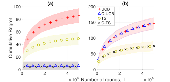
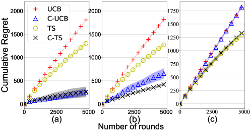
Figure 5: Cumulative regret for UCB, C-UCB, TS and C-TS corresponding to the problem shown in Table 4. For the setting (a) in Table 4, Arm 1 is optimal and Arm 2 is non-competitive, in setting (b) of Table 4 Arm 2 is optimal while Arm 1 is competitive.

Consider the example shown in Table 1, with the top row showing the pseudo-rewards, which are known to the player, and the bottom row showing two possible joint probability distributions (a) and (b), which are unknown to the player. We show the simulation result of our proposed algorithms C-UCB, C-TS against UCB, TS in Figure 5 for the setting considered in Table 1.

Case (a): Bounded regret. For the probability distribution (a), notice that Arm 1 is optimal with μ1=0.6,μ2=0.4formulae-sequencesubscript𝜇10.6subscript𝜇20.4\mu_{1}=0.6,\mu_{2}=0.4. Moreover, ϕ2,1=0.4×0.7+0.6×0.4=0.52subscriptitalic-ϕ210.40.70.60.40.52\phi_{2,1}=0.4\times 0.7+0.6\times 0.4=0.52. Since ϕ2,1<μ1subscriptitalic-ϕ21subscript𝜇1\phi_{2,1}<\mu_{1}, Arm 2 is non-competitive. Hence, in Figure 5(a), we see that our proposed C-UCB and C-TS Algorithms achieve bounded regret, whereas UCB, TS show logarithmic regret.

Case (b): All competitive arms. For the probability distribution (b), Arm 2 is optimal with μ2=0.5subscript𝜇20.5\mu_{2}=0.5 and μ1=0.4subscript𝜇10.4\mu_{1}=0.4. The expected pseudo-reward of arm 1 w.r.t to arm 2 in this case is ϕ1,2=0.8×0.5+0.5×0.5=0.65subscriptitalic-ϕ120.80.50.50.50.65\phi_{1,2}=0.8\times 0.5+0.5\times 0.5=0.65. Since ϕ1,2>μ2subscriptitalic-ϕ12subscript𝜇2\phi_{1,2}>\mu_{2}, the sub-optimal arm (i.e., Arm 1) is competitive and hence C-UCB and C-TS also end up exploring Arm 1. Due to this we see that C-UCB, C-TS achieve a regret similar to UCB, TS in Figure 5(b). C-TS has empirically smaller regret than C-UCB as Thompson Sampling performs better empirically than the UCB algorithm. The design of our C-Bandit approach allows the use of any other bandit algorithm in the last step, e.g., KL-UCB.

5.2 Simulations for the latent random source model in Section 2.3
Refer to caption
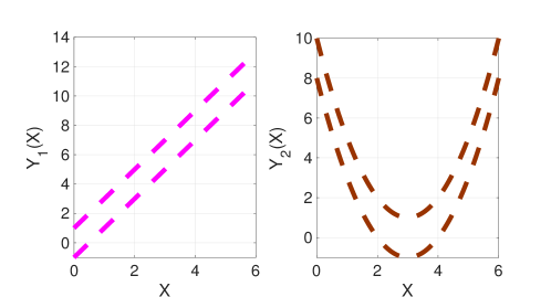
Figure 6: Rewards corresponding to the two arms are correlated through a random variable X𝑋X lying in (0,6)06(0,6). The lines represent lower and upper bounds on reward of Arms 1 ,Y1(X)subscript𝑌1𝑋Y_{1}(X), and 2, Y2(X)subscript𝑌2𝑋Y_{2}(X), given the realization of random variable X𝑋X.
Refer to caption
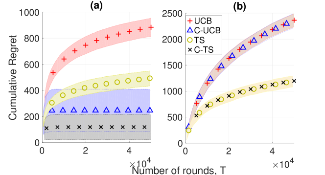
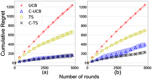
Figure 7: Simulation results for the example shown in Figure 6. In (a), XBeta(1,1)similar-to𝑋Beta11X\sim\text{Beta}(1,1) and in (b) XBeta(1.5,5)similar-to𝑋Beta1.55X\sim\text{Beta}(1.5,5). In case (a), Arm 1 is optimal while Arm 2 is non-competitive (C = 1), due to which we see that C-UCB and C-TS obtain bounded regret. Arm 2 is optimal for the distribution in (b) and Arm 1 is competitive, due to which C=2𝐶2C=2 and we see that C-UCB and C-TS attain a performance similar to UCB and TS.

We now show the performance of C-UCB and C-TS against UCB, TS for the model considered in Section 2.3, where rewards corresponding to different arms are correlated through a latent random variable X𝑋X. We consider a setting where reward obtained from Arm 1, given a realization x𝑥x of X𝑋X, is bounded between 2x12𝑥12x-1 and 2x+12𝑥12x+1, i.e., 2X1Y1(X)2X+12𝑋1subscript𝑌1𝑋2𝑋12X-1\leq Y_{1}(X)\leq 2X+1. Similarly, conditional reward of Arm 2 is, (3X)21Y2(X)(3X)2+1superscript3𝑋21subscript𝑌2𝑋superscript3𝑋21(3-X)^{2}-1\leq Y_{2}(X)\leq(3-X)^{2}+1. Figure 6 demonstrates these upper and lower bounds on Yk(X)subscript𝑌𝑘𝑋Y_{k}(X). We run C-UCB, C-TS, TS and UCB for this setting for two different distributions of X𝑋X. For the simulations, we set the conditional reward of both the arms to be distributed uniformly between the upper and lower bounds, however this information is not known to the Algorithms.

Case (a): XBeta(1,1)similar-to𝑋Beta11X\sim\text{Beta}(1,1). When X𝑋X is distributed as XBeta(1,1)similar-to𝑋Beta11X\sim\text{Beta}(1,1), Arm 1 is optimal while Arm 2 is non-competitive. Due to this, we observe that C-UCB and C-TS achieve bounded regret in Figure 7(a).

Case (b): XBeta(1.5,5)similar-to𝑋Beta1.55X\sim\text{Beta}(1.5,5). In the scenario where X𝑋X has the distribution Beta(1.5,5)Beta1.55\text{Beta}(1.5,5), Arm 2 is optimal while Arm 1 is competitive. Due to this, C-UCB and C-TS do not stop exploring Arm 1 in finite time and we see the cumulative regret similar to UCB, TS in Figure 7(b).

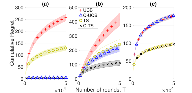
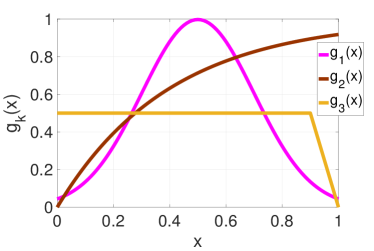
Our next simulation result considers a setting where the known upper and lower bounds on Yk(X)subscript𝑌𝑘𝑋Y_{k}(X) match and the reward Yksubscript𝑌𝑘Y_{k} corresponding to a realization of X𝑋X is deterministic, i.e., Yk(X)=gk(X)subscript𝑌𝑘𝑋subscript𝑔𝑘𝑋Y_{k}(X)=g_{k}(X). We show our simulation results for the reward functions described in Figure 8 with three different distributions of X𝑋X. Corresponding to XBeta(4,4)similar-to𝑋Beta44X\sim\text{Beta}(4,4), Arm 1 is optimal and Arms 2,3 are non-competitive leading to bounded regret for C-UCB, C-TS in Figure 9(a). In setting (b), we consider XBeta(2,5)similar-to𝑋Beta25X\sim\text{Beta}(2,5) in which Arm 1 is optimal, Arm 2 is competitive and Arm 3 is non-competitive. Due to this, our proposed C-UCB and C-TS Algorithms stop pulling Arm 3 after some time and hence achieve significantly reduced regret relative to UCB in Figure 9(b). For third scenario (c), we set XBeta(1,5)similar-to𝑋Beta15X\sim\text{Beta}(1,5), which makes Arm 3 optimal while Arms 1 and 2 are competitive. Hence, our algorithms explore both the sub-optimal arms and have a regret comparable to that of UCB, TS in Figure 9(c).
Refer to caption
Figure 8: Reward Functions used for the simulation results presented in Figure 9. The reward gk(X)subscript𝑔𝑘𝑋g_{k}(X) is a function of a latent random variable X𝑋X. For instance, when X=0.5𝑋0.5X=0.5, reward from Arms 1,2 and 3 are g1(X)=1subscript𝑔1𝑋1g_{1}(X)=1, g2(X)=0.7135subscript𝑔2𝑋0.7135g_{2}(X)=0.7135 and g3(X)=0.5subscript𝑔3𝑋0.5g_{3}(X)=0.5.
Refer to caption
Figure 9: The cumulative regret of C-UCB and C-TS depend on C𝐶C, the number of competitive arms. The value of C𝐶C depends on the unknown joint probability distribution of rewards and is not known beforehand. We consider a setup where C=1𝐶1C=1 in (a), C=2𝐶2C=2 in (b) and C=3𝐶3C=3 in (c). Our proposed algorithm pull only the C1𝐶1C-1 competitive sub-optimal arms O(logT)O𝑇\mathrm{O}(\log T) times, as opposed to UCB, TS that pull all K1𝐾1K-1 sub-optimal arms O(logT)O𝑇\mathrm{O}(\log T) times. Due to this, we see that our proposed algorithms achieve bounded regret when C=1𝐶1C=1. When C=3𝐶3C=3, our proposed algorithms perform as well as the UCB, TS algorithms.

6 Experiments

We now show the performance of our proposed algorithms in real-world settings. Through the use of MovieLens and Goodreads datasets, we demonstrate how the correlated MAB framework can be used in practical settings for recommendation system applications. In such systems, it is possible to use the prior available data (from a certain population) to learn the correlation structure in the form of pseudo-rewards. When trying to design a campaign to maximize user engagement in a new unknown demographic, the learned correlation information in the form of pseudo-rewards can help significantly reduce the regret as we show from our results described below.

6.1 Experiments on the MovieLens dataset

The MovieLens dataset [31] contains a total of 1M ratings for a total of 3883 Movies rated by 6040 Users. Each movie is rated on a scale of 1-5 by the users. Moreover, each movie is associated with one (and in some cases, multiple) genres. For our experiments, of the possibly several genres associated with each movie, one is picked uniformly at random. To perform our experiments, we split the data into two parts, with the first half containing ratings of the users who provided the most number of ratings. This half is used to learn the pseudo-reward entries, the other half is the test set which is used to evaluate the performance of the proposed algorithms. Doing such a split ensures that the rating distribution is different in the training and test data.
Refer to caption
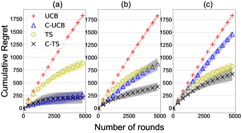
Figure 10: Cumulative regret for UCB, C-UCB, TS and C-TS for the application of recommending the best genre in the Movielens dataset, where p𝑝p fraction of the pseudo-entries are replaced with maximum reward i.e.,5i.e.,5. In (a),p=0.25𝑎𝑝0.25(a),p=0.25, for (b),p=0.50𝑏𝑝0.50(b),p=0.50 and p=0.7𝑝0.7p=0.7 in (c)𝑐(c). The value of C𝐶C is 4,114114,11 and 131313 in (a),(b)𝑎𝑏(a),(b) and (c)𝑐(c) respectively. As C𝐶C is smaller than K𝐾K (i.e., 181818) in each case, we see that C-UCB and C-TS outperform UCB and TS significantly.

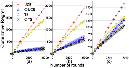
Recommending the Best Genre. In our first experiment, the goal is to provide the best genre recommendations to a population with unknown demographic. We use the training dataset to learn the pseudo-reward entries. The pseudo-reward entry s,k(r)subscript𝑠𝑘𝑟s_{\ell,k}(r) is evaluated by taking the empirical average of the ratings of genre \ell that are rated by the users who rated genre k𝑘k as r𝑟r. To capture the fact that it might not be possible in practice to fill all pseudo-reward entries, we randomly remove p𝑝p-fraction of the pseudo-reward entries. The removed pseudo-reward entries are replaced by the maximum possible rating, i.e., 555 (as that gives a natural upper bound on the conditional mean reward). Using these pseudo-rewards, we evaluate our proposed algorithms on the test data. Upon recommending a particular genre (arm), the rating (reward) is obtained by sampling one of the ratings for the chosen arm in the test data. Our experimental results for this setting are shown in Figure 10, with p=0.25,0.50𝑝0.250.50p=0.25,0.50 and 0.700.700.70 (i.e., fraction of pseudo-reward entries that are removed). We see that the proposed C-UCB and C-TS algorithms significantly outperform UCB and TS in all three settings. For each of the three cases we also evaluate the value of C𝐶C (which is unknown to the algorithm), by always pulling the optimal arm and finding the size of empirically competitive set at T=5000𝑇5000T=5000. The value of C𝐶C turned out to be 4,114114,11 and 131313 for p=0.25,0.50𝑝0.250.50p=0.25,0.50 and 0.700.700.70. As C<18𝐶18C<18 in each case, some of the 18 arms are stopped being pulled after some time and due to this, C-UCB and C-TS significantly outperform UCB and TS respectively. This shows that even when only a subset of the correlations are known, it is possible to exploit them to improve the performance of classical bandit algorithms.
Refer to caption
Figure 11: Cumulative regret of UCB, C-UCB, TS and C-TS for providing the best movie recommendations in the Movielens dataset. Each pseudo-reward entry is added by 0.10.10.1 in (a), 0.40.40.4 in (b) and 0.60.60.6 in (c). The value of C𝐶C is 6,246246,24 and 393939 in (a),(b)𝑎𝑏(a),(b) and (c)𝑐(c) respectively. As C𝐶C is smaller than K𝐾K (i.e., 505050) in each case, we see the superior performance of C-UCB, C-TS over UCB and TS.

Recommending the Best Movie. We now consider the goal of providing the best movie recommendations to the population. To do so, we consider the 50 most rated movies in the dataset. containing 109,804 user-ratings given by 6,025 users. In the testing phase, the goal is to recommend one of these 50 movies to each user. As was the case in previous experiment, we learn the pseudo-reward entries from the training data. Instead of using the learned pseudo-reward directly, we add a safety buffer to each of the pseudo-reward entry; i.e., we set the pseudo-reward as the empirical conditional mean plus the safety buffer. Adding a buffer will be needed in practice, as the conditional expectations learned from the training data are likely to have some noise and adding a safety buffer allows us to make sure that pseudo-rewards constitute an upper bound on the conditional expectations. Our experimental result in Figure 11 shows the performance of C-UCB and C-TS relative to UCB for this setting with safety buffer set to 0.10.10.1 in Figure 11(a), 0.40.40.4 in Figure 11(b) and 0.60.60.6 in Figure 11(c). In all three cases, even after addition of safety buffers, our proposed C-UCB and C-TS algorithms outperform the UCB algorithm.

6.2 Experiments on the Goodreads dataset

The Goodreads dataset [32] contains the ratings for 1,561,465 books by a total of 808,749 users. Each rating is on a scale of 1-5. For our experiments, we only consider the poetry section and focus on the goal of providing best poetry recommendations to the whole population whose demographics is unknown. The poetry dataset has 36,182 different poems rated by 267,821 different users. We do the pre-processing of goodreads dataset in the same manner as that of the MovieLens dataset, by splitting the dataset into two halves, train and test. The train dataset contains the ratings of the users with most number of recommendations.
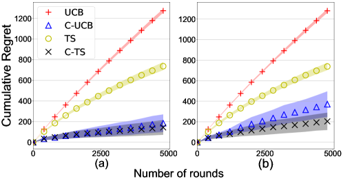
Refer to caption
Figure 12: Cumulative regret of UCB, C-UCB, TS and C-TS for providing best poetry book recommendation in the Goodreads dataset. Every pseudo-reward entry is added by q𝑞q and p𝑝p fraction of the pseudo-reward entries are removed, with (a) p=0.1,q=0.1formulae-sequence𝑝0.1𝑞0.1p=0.1,q=0.1 and (b) p=0.3,q=0.1formulae-sequence𝑝0.3𝑞0.1p=0.3,q=0.1. The value of C𝐶C is 888 and 111111 in (a)𝑎(a) and (b)𝑏(b) respectively. As C𝐶C is much smaller than K𝐾K (i.e., 252525) in each case, we see that C-UCB and C-TS outperform UCB and TS significantly.

Recommending the best poetry book. We consider the 25 most rated books in the dataset and use these as the set of arms to recommend in the testing phase. These 25 poems have 349,523 user-ratings given by 171,433 users. As with the MovieLens dataset, the pseudo-reward entries are learned on the training data. In practical situations it might not be possible to obtain all pseudo-reward entries. Therefore, we randomly select p𝑝p fraction of the pseudo-reward entries and replace them with maximum possible reward (i.e. 555). Among the remaining pseudo-reward entries we add a safety buffer of q𝑞q to each entry. Our result in Figure 12 shows the performance of C-UCB and C-TS relative to UCB and TS in two scenarios. In scenario (a), 10%percent1010\% of the pseudo-reward entries are replaced by 555 and remaining are padded with a safety buffer of 0.10.10.1. For case (b), 30%percent3030\% entries are replaced by 555 and safety buffer is 0.10.10.1. Under both cases, our proposed C-UCB and C-TS algorithms are able to outperform UCB and TS significantly.

6.3 Pseudo-rewards learned on a smaller dataset

In our previous set of experiments, half of the dataset was used to learn the pseudo-reward entries. We did additional experiments in a setup where only 10%percent1010\% of the data was used for learning the pseudo-reward entries and tested our algorithms on the remaining dataset. On doing so, we observed that C-UCB and C-TS were still able to outperform UCB and TS in most of our experimental setups. One setting in which the performance of C-UCB was similar to that of UCB is in a scenario where each pseudo-reward entry was padded by 0.60.60.6. As the padding was large, the C-UCB algorithm was not able to identify many arms as non-competitive, leading to a performance that is similar to that of UCB. In all other scenarios, we noted that C-UCB and C-TS significantly outperformed UCB and TS, suggesting that even when smaller dataset is used for learning pseudo-rewards, the C-UCB and C-TS can be quite effective. The results are presented in Figure 13, Figure 14 and Figure 15.
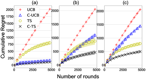
Refer to caption
Figure 13: Cumulative regret for UCB, C-UCB, TS and C-TS for the application of recommending the best genre in the Movielens dataset, where p𝑝p fraction of the pseudo-entries are replaced with maximum reward i.e.,5i.e.,5. In (a),p=0.25𝑎𝑝0.25(a),p=0.25, for (b),p=0.50𝑏𝑝0.50(b),p=0.50 and p=0.7𝑝0.7p=0.7 in (c)𝑐(c). We used 10%percent1010\% of the dataset to learn the pseudo-reward entry and the algorithms are tested on the remaining dataset. The value of C𝐶C is 5,115115,11 and 151515 in (a),(b)𝑎𝑏(a),(b) and (c)𝑐(c) respectively. As C𝐶C is smaller than K𝐾K (i.e., 181818) in each case, we see that C-UCB and C-TS outperform UCB and TS significantly. Note that the value of C𝐶C is larger in the case where only 10%percent1010\% data is used for learning the pseudo-reward.
Refer to caption
Figure 14: Cumulative regret of UCB, C-UCB, TS and C-TS for providing the best movie recommendations in the Movielens dataset. In this experiment 10%percent1010\% of the dataset is used for learning the pseudo-reward entry and the algorithms are tested on the remaining dataset. Each pseudo-reward entry is added by 0.10.10.1 in (a), 0.40.40.4 in (b) and 0.60.60.6 in (c). The value of C𝐶C is 14,29142914,29 and 424242 in (a),(b)𝑎𝑏(a),(b) and (c)𝑐(c) respectively. Note that the value of C𝐶C is larger in the case where only 10%percent1010\% data is used for learning the pseudo-reward. As C𝐶C is still smaller than K𝐾K (i.e., 505050) in each case, we see the superior performance of C-UCB, C-TS over UCB and TS.
Refer to caption
Figure 15: Cumulative regret of UCB, C-UCB, TS and C-TS for providing best poetry book recommendation in the Goodreads dataset. We used 10%percent1010\% of the dataset to learn the pseudo-reward entry and the algorithms are tested on the remaining dataset. Every pseudo-reward entry is added by q𝑞q and p𝑝p fraction of the pseudo-reward entries are removed, with (a) p=0.1,q=0.1formulae-sequence𝑝0.1𝑞0.1p=0.1,q=0.1 and (b) p=0.3,q=0.1formulae-sequence𝑝0.3𝑞0.1p=0.3,q=0.1. The value of C𝐶C is 777 and 121212 in (a)𝑎(a) and (b)𝑏(b) respectively. As C𝐶C is much smaller than K𝐾K (i.e., 252525) in each case, we see that C-UCB and C-TS outperform UCB and TS significantly.

7 Conclusion

This work presents a new correlated Multi-Armed bandit problem in which rewards obtained from different arms are correlated. We capture this correlation through the knowledge of pseudo-rewards. These pseudo-rewards, which represent upper bound on conditional mean rewards, could be known in practice from either domain knowledge or learned from prior data. Using the knowledge of these pseudo-rewards, we the propose C-Bandit algorithm which fundamentally generalizes any classical bandit algorithm to the correlated multi-armed bandit setting. A key strength of our paper is that it allows pseudo-rewards to be loose (in case there is not much prior information) and even then our C-Bandit algorithms adapt and provide performance at least as good as that of classical bandit algorithms.

We provide a unified method to analyze the regret of C-Bandit algorithms. In particular, the analysis shows that C-UCB ends up pulling non-competitive arms only O(1)O1\mathrm{O}(1) times; i.e., they stop pulling certain arms after a finite time t𝑡t. Due to this, C-UCB pulls only C1K1𝐶1𝐾1C-1\leq K-1 of the K1𝐾1K-1 sub-optimal arms O(logT)O𝑇\mathrm{O}(\log T) times, as opposed to UCB that pulls all K1𝐾1K-1 sub-optimal arms O(logT)O𝑇\mathrm{O}(\log T) times. In this sense, our C-Bandit algorithms reduce a K𝐾K-armed bandit to a C𝐶C-armed bandit problem. We present several cases where C=1𝐶1C=1 for which C-UCB achieves bounded regret. For the special case when rewards are correlated through a latent random variable X𝑋X, we provide a lower bound showing that bounded regret is possible only when C=1𝐶1C=1; if C>1𝐶1C>1, then O(logT)O𝑇\mathrm{O}(\log T) regret is not possible to avoid. Thus, our C-UCB algorithm achieves bounded regret whenever possible. Simulation results validate the theoretical findings and we perform experiments on Movielens and Goodreads datasets to demonstrate the applicability of our framework in the context of recommendation systems. The experiments on real-world datasets show that our C-UCB and C-TS algorithms significantly outperform the UCB and TS algorithms.

There are several interesting open problems and extensions of this work, some of which we describe below.

Extension to light tailed and heavy tailed rewards In this work, we assume that the rewards have a bounded support. The algorithm and analysis can be extended to settings with sub-gaussian rewards as well. In particular, in step 3 of the algorithm, one would play UCB/TS for sub-gaussian rewards. For instance, the UCB index in the scenario of sub-gaussian rewards can be redefined as μ^k+2σ2logtnk(t)subscript^𝜇𝑘2superscript𝜎2𝑡subscript𝑛𝑘𝑡\hat{\mu}_{k}+\sqrt{\frac{2\sigma^{2}\log t}{n_{k}(t)}}, where σ𝜎\sigma is the sub-Gaussianity parameter of the reward distribution. Similar regret bounds will hold in this setting as well because the Hoeffding’s inequality used in our regret analysis is valid for sub-Gaussian rewards as well. For heavy-tailed rewards, the Hoeffding’s inequality is not valid. Due to which, one would need to construct confidence bounds for UCB in a different manner as done in [33]. On doing so, the C-Bandit algorithm can be employed in heavy-tailed reward settings. However, the regret analysis may not extend directly as one would need to use modified concentration inequalities to obtain bounds on mean reward of arm k𝑘k as done in Lemma 1 of [33].

Designing better algorithms. While our proposed algorithms are order-optimal for the model in Section 2.3, they do not match the pre-log constants in the lower bound of the regret. It may be possible to design algorithms that have smaller pre-log constants in their regret upper bound. Further discussion along these lines is presented in Appendix F. A key advantage of our approach is that our algorithms are easy to implement and they incorporate the classical bandit algorithms nicely for the problem of correlated multi-armed bandits.

Best-Arm Identification. We plan to study the problem of best-arm identification in the correlated multi-armed bandit setting, i.e., to identify the best arm with a confidence 1δ1𝛿1-\delta in as few samples as possible. Since rewards are correlated with each other, we believe the sample complexity can be significantly improved relative to state of the art algorithms, such as LIL-UCB [34, 35], which are designed for classical multi-armed bandits. Another open direction is to improve the C-Bandit algorithm to make sure that it achieves bounded regret whenever possible in the general framework studied in this paper.

8 Acknowledgments

This work was partially supported by the NSF through grants CCF-1840860 and CCF-2007834, the Siebel Energy Institute, the Carnegie Bosch Institute, the Manufacturing Futures Initiative, and the CyLab IoT Initiative. In addition, Samarth Gupta was supported by the CyLab Presidential Fellowship and the David H. Barakat and LaVerne Owen-Barakat CIT Dean’s Fellowship.

References

  • [1] T. L. Lai and H. Robbins, “Asymptotically efficient adaptive allocation rules,” Advances in applied mathematics, vol. 6, no. 1, pp. 4–22, 1985.
  • [2] S. Agrawal and N. Goyal, “Analysis of thompson sampling for the multi-armed bandit problem,” in Conference on Learning Theory, pp. 39–1, 2012.
  • [3] A. Garivier and O. Cappé, “The kl-ucb algorithm for bounded stochastic bandits and beyond,” in Proceedings of the 24th annual Conference On Learning Theory, pp. 359–376, 2011.
  • [4] S. S. Villar, J. Bowden, and J. Wason, “Multi-armed bandit models for the optimal design of clinical trials: benefits and challenges,” Statistical science: a review journal of the Institute of Mathematical Statistics, vol. 30, no. 2, p. 199, 2015.
  • [5] D. Agarwal, B.-C. Chen, and P. Elango, “Explore/exploit schemes for web content optimization,” in Data Mining, 2009. ICDM’09. Ninth IEEE International Conference on, pp. 1–10, IEEE, 2009.
  • [6] C. Tekin and E. Turgay, “Multi-objective contextual multi-armed bandit problem with a dominant objective,” arXiv preprint arXiv:1708.05655, 2017.
  • [7] J. Nino-Mora, Stochastic scheduling. In Encyclopedia of Optimization, pp. 3818–3824. New York: Springer, 2 ed., 2009.
  • [8] S. Krishnasamy, R. Sen, R. Johari, and S. Shakkottai, “Regret of queueing bandits,” CoRR, vol. abs/1604.06377, 2016.
  • [9] G. Joshi, Efficient Redundancy Techniques to Reduce Delay in Cloud Systems. PhD thesis, Massachusetts Institute of Technology, June 2016.
  • [10] J. White, Bandit algorithms for website optimization. " O’Reilly Media, Inc.", 2012.
  • [11] L. Zhou, “A survey on contextual multi-armed bandits,” CoRR, vol. abs/1508.03326, 2015.
  • [12] A. Agarwal, D. Hsu, S. Kale, J. Langford, L. Li, and R. E. Schapire, “Taming the monster: A fast and simple algorithm for contextual bandits,” in Proceedings of the International Conference on Machine Learning (ICML), pp. 1638–1646, 2014.
  • [13] R. Combes, S. Magureanu, and A. Proutiere, “Minimal exploration in structured stochastic bandits,” in Advances in Neural Information Processing Systems, pp. 1763–1771, 2017.
  • [14] T. Lattimore and R. Munos, “Bounded regret for finite-armed structured bandits,” in Advances in Neural Information Processing Systems, pp. 550–558, 2014.
  • [15] Y. Abbasi-Yadkori, D. Pál, and C. Szepesvári, “Improved algorithms for linear stochastic bandits,” in Advances in Neural Information Processing Systems, pp. 2312–2320, 2011.
  • [16] V. Dani, T. P. Hayes, and S. M. Kakade, “Stochastic linear optimization under bandit feedback,” in Proceedings on the Conference on Learning Theory (COLT), 2008.
  • [17] S. Gupta, G. Joshi, and O. Yağan, “Correlated multi-armed bandits with a latent random source,” in ICASSP 2020-2020 IEEE International Conference on Acoustics, Speech and Signal Processing (ICASSP), pp. 3572–3576, IEEE, 2020.
  • [18] S. Gupta, S. Chaudhari, S. Mukherjee, G. Joshi, and O. Yağan, “A unified approach to translate classical bandit algorithms to the structured bandit setting,” 2018.
  • [19] S. Filippi, O. Cappe, A. Garivier, and C. Szepesvári, “Parametric bandits: The generalized linear case,” in Advances in Neural Information Processing Systems, pp. 586–594, 2010.
  • [20] S. Magureanu, R. Combes, and A. Proutiere, “Lipschitz bandits: Regret lower bounds and optimal algorithms,” arXiv preprint arXiv:1405.4758, 2014.
  • [21] O. Atan, C. Tekin, and M. van der Schaar, “Global multi-armed bandits with hölder continuity,” in AISTATS, 2015.
  • [22] Z. Wang, R. Zhou, and C. Shen, “Regional multi-armed bandits,” in AISTATS, 2018.
  • [23] S. Pandey, D. Chakrabarti, and D. Agarwal, “Multi-armed bandit problems with dependent arms,” in Proceedings of the International Conference on Machine Learning, pp. 721–728, 2007.
  • [24] R. Combes and A. Proutiere, “Unimodal bandits: Regret lower bounds and optimal algorithms,” in International Conference on Machine Learning, pp. 521–529, 2014.
  • [25] C. Trinh, E. Kaufmann, C. Vernade, and R. Combes, “Solving bernoulli rank-one bandits with unimodal thompson sampling,” in Algorithmic Learning Theory, pp. 862–889, PMLR, 2020.
  • [26] M. A. Qureshi and C. Tekin, “Fast learning for dynamic resource allocation in ai-enabled radio networks,” IEEE Transactions on Cognitive Communications and Networking, vol. 6, no. 1, pp. 95–110, 2019.
  • [27] M. A. Qureshi and C. Tekin, “Online bayesian learning for rate selection in millimeter wave cognitive radio networks,” in IEEE INFOCOM 2020-IEEE Conference on Computer Communications, pp. 1449–1458, IEEE, 2020.
  • [28] H. Gupta, A. Eryilmaz, and R. Srikant, “Link rate selection using constrained thompson sampling,” in IEEE INFOCOM 2019-IEEE Conference on Computer Communications, pp. 739–747, IEEE, 2019.
  • [29] P. Auer, N. Cesa-Bianchi, and P. Fischer, “Finite-time analysis of the multiarmed bandit problem,” Machine learning, vol. 47, no. 2-3, pp. 235–256, 2002.
  • [30] S. Agrawal and N. Goyal, “Further optimal regret bounds for thompson sampling,” in Artificial Intelligence and Statistics, pp. 99–107, 2013.
  • [31] F. M. Harper and J. A. Konstan, “The movielens datasets: History and context,” ACM Transactions on Interactive Intelligent Systems (TiiS), vol. 5, 4, Article 19, 2015.
  • [32] M. Wan and J. McAuley, “Item recommendation on monotonic behavior chains,” in Proceedings of the 12th ACM Conference on Recommender Systems, pp. 86–94, ACM, 2018.
  • [33] S. Bubeck, N. Cesa-Bianchi, and G. Lugosi, “Bandits with heavy tail,” IEEE Transactions on Information Theory, vol. 59, no. 11, pp. 7711–7717, 2013.
  • [34] K. Jamieson and R. Nowak, “Best-arm identification algorithms for multi-armed bandits in the fixed confidence setting,” in Proceedings on the Annual Conference on Information Sciences and Systems (CISS), pp. 1–6, March 2014.
  • [35] K. Jamieson, M. Malloy, R. Nowak, and S. Bubeck, “lil’ucb: An optimal exploration algorithm for multi-armed bandits,” in Conference on Learning Theory, pp. 423–439, 2014.
  • [36] T. Lattimore, “Instance dependent lower bounds.” http://banditalgs.com/2016/09/30/instance-dependent-lower-bounds/.
  • [37] A. B. Tsybakov, Introduction to Nonparametric Estimation. Springer Publishing Company, Incorporated, 1st ed., 2008.
  • [38] J. Bretagnolle and C. Huber, “Estimation des densitiés: risque minimax. z. für wahrscheinlichkeitstheorie und verw,” Geb., vol. 47, pp. 199–137, 1979.
  • [39] B. Van Parys and N. Golrezaei, “Optimal learning for structured bandits,” 2020.
  • [40] T. L. Graves and T. L. Lai, “Asymptotically efficient adaptive choice of control laws incontrolled markov chains,” SIAM journal on control and optimization, vol. 35, no. 3, pp. 715–743, 1997.

A Standard Results from Previous Works

Fact 1 (Hoeffding’s inequality).

Let Z1,Z2Znsubscript𝑍1subscript𝑍2subscript𝑍𝑛Z_{1},Z_{2}\ldots Z_{n} be i.i.d random variables bounded between [a,b]:aZib:𝑎𝑏𝑎subscript𝑍𝑖𝑏[a,b]:a\leq Z_{i}\leq b, then for any δ>0𝛿0\delta>0, we have

Pr(|i=1nZin𝔼[Zi]|δ)exp(2nδ2(ba)2).Prsuperscriptsubscript𝑖1𝑛subscript𝑍𝑖𝑛𝔼delimited-[]subscript𝑍𝑖𝛿2𝑛superscript𝛿2superscript𝑏𝑎2\Pr\left(\left|\frac{\sum_{i=1}^{n}Z_{i}}{n}-\mathbb{E}\left[{Z_{i}}\right]\right|\geq\delta\right)\leq\exp\left(\frac{-2n\delta^{2}}{(b-a)^{2}}\right).
Lemma 1 (Standard result used in bandit literature).

If μ^k,nk(t)subscript^𝜇𝑘subscript𝑛𝑘𝑡\hat{\mu}_{k,n_{k}(t)} denotes the empirical mean of arm k𝑘k by pulling arm k𝑘k nk(t)subscript𝑛𝑘𝑡n_{k}(t) times through any algorithm and μksubscript𝜇𝑘\mu_{k} denotes the mean reward of arm k𝑘k, then we have

Pr(μ^k,nk(t)μkϵ,τ2nk(t)τ1)s=τ1τ2exp(2sϵ2).Prsubscript^𝜇𝑘subscript𝑛𝑘𝑡subscript𝜇𝑘italic-ϵsubscript𝜏2subscript𝑛𝑘𝑡subscript𝜏1superscriptsubscript𝑠subscript𝜏1subscript𝜏22𝑠superscriptitalic-ϵ2\Pr\left(\hat{\mu}_{k,n_{k}(t)}-\mu_{k}\geq\epsilon,\tau_{2}\geq n_{k}(t)\geq\tau_{1}\right)\leq\sum_{s=\tau_{1}}^{\tau_{2}}\exp\left(-2s\epsilon^{2}\right).
Proof.

Let Z1,Z2,Ztsubscript𝑍1subscript𝑍2subscript𝑍𝑡Z_{1},Z_{2},...Z_{t} be the reward samples of arm k𝑘k drawn separately. If the algorithm chooses to play arm k𝑘k for mthsuperscript𝑚𝑡m^{th} time, then it observes reward Zmsubscript𝑍𝑚Z_{m}. Then the probability of observing the event μ^k,nk(t)μkϵ,τ2nk(t)τ1formulae-sequencesubscript^𝜇𝑘subscript𝑛𝑘𝑡subscript𝜇𝑘italic-ϵsubscript𝜏2subscript𝑛𝑘𝑡subscript𝜏1\hat{\mu}_{k,n_{k}(t)}-\mu_{k}\geq\epsilon,\tau_{2}\geq n_{k}(t)\geq\tau_{1} can be upper bounded as follows,

Pr(μ^k,nk(t)μkϵ,τ2nk(t)τ1)Prsubscript^𝜇𝑘subscript𝑛𝑘𝑡subscript𝜇𝑘italic-ϵsubscript𝜏2subscript𝑛𝑘𝑡subscript𝜏1\displaystyle\Pr\left(\hat{\mu}_{k,n_{k}(t)}-\mu_{k}\geq\epsilon,\tau_{2}\geq n_{k}(t)\geq\tau_{1}\right) =Pr((i=1nk(t)Zink(t)μkϵ),τ2nk(t)τ1)absentPrsuperscriptsubscript𝑖1subscript𝑛𝑘𝑡subscript𝑍𝑖subscript𝑛𝑘𝑡subscript𝜇𝑘italic-ϵsubscript𝜏2subscript𝑛𝑘𝑡subscript𝜏1\displaystyle=\Pr\left(\left(\frac{\sum_{i=1}^{n_{k}(t)}Z_{i}}{n_{k}(t)}-\mu_{k}\geq\epsilon\right),\tau_{2}\geq n_{k}(t)\geq\tau_{1}\right) (22)
Pr((m=τ1τ2i=1mZimμkϵ),τ2nk(t)τ1)absentPrsuperscriptsubscript𝑚subscript𝜏1subscript𝜏2superscriptsubscript𝑖1𝑚subscript𝑍𝑖𝑚subscript𝜇𝑘italic-ϵsubscript𝜏2subscript𝑛𝑘𝑡subscript𝜏1\displaystyle\leq\Pr\left(\left(\bigcup_{m=\tau_{1}}^{\tau_{2}}\frac{\sum_{i=1}^{m}Z_{i}}{m}-\mu_{k}\geq\epsilon\right),\tau_{2}\geq n_{k}(t)\geq\tau_{1}\right) (23)
Pr(m=τ1τ2i=1mZimμkϵ)absentPrsuperscriptsubscript𝑚subscript𝜏1subscript𝜏2superscriptsubscript𝑖1𝑚subscript𝑍𝑖𝑚subscript𝜇𝑘italic-ϵ\displaystyle\leq\Pr\left(\bigcup_{m=\tau_{1}}^{\tau_{2}}\frac{\sum_{i=1}^{m}Z_{i}}{m}-\mu_{k}\geq\epsilon\right) (24)
s=τ1τ2exp(2sϵ2).absentsuperscriptsubscript𝑠subscript𝜏1subscript𝜏22𝑠superscriptitalic-ϵ2\displaystyle\leq\sum_{s=\tau_{1}}^{\tau_{2}}\exp\left(-2s\epsilon^{2}\right). (25)

Lemma 2 (From Proof of Theorem 1 in [29]).

Let Ik(t)subscript𝐼𝑘𝑡I_{k}(t) denote the UCB index of arm k𝑘k at round t𝑡t, and μk=𝔼[gk(X)]subscript𝜇𝑘𝔼delimited-[]subscript𝑔𝑘𝑋\mu_{k}=\mathbb{E}\left[{g_{k}(X)}\right] denote the mean reward of that arm. Then, we have

Pr(μk>Ik(t))t3.Prsubscript𝜇𝑘subscript𝐼𝑘𝑡superscript𝑡3\Pr(\mu_{k}>I_{k}(t))\leq t^{-3}.

Observe that this bound does not depend on the number nk(t)subscript𝑛𝑘𝑡n_{k}(t) of times arm k𝑘k is pulled. UCB index is defined in equation (6) of the main paper.

Proof.

This proof follows directly from [29]. We present the proof here for completeness as we use this frequently in the paper.

Pr(μk>Ik(t))Prsubscript𝜇𝑘subscript𝐼𝑘𝑡\displaystyle\Pr(\mu_{k}>I_{k}(t)) =Pr(μk>μ^k,nk(t)+2logtnk(t))absentPrsubscript𝜇𝑘subscript^𝜇𝑘subscript𝑛𝑘𝑡2𝑡subscript𝑛𝑘𝑡\displaystyle=\Pr\left(\mu_{k}>\hat{\mu}_{k,n_{k}(t)}+\sqrt{\frac{2\log t}{n_{k}(t)}}\right) (26)
m=1tPr(μk>μ^k,m+2logtm)absentsuperscriptsubscript𝑚1𝑡Prsubscript𝜇𝑘subscript^𝜇𝑘𝑚2𝑡𝑚\displaystyle\leq\sum_{m=1}^{t}\Pr\left(\mu_{k}>\hat{\mu}_{k,m}+\sqrt{\frac{2\log t}{m}}\right) (27)
=m=1tPr(μ^k,mμk<2logtm)absentsuperscriptsubscript𝑚1𝑡Prsubscript^𝜇𝑘𝑚subscript𝜇𝑘2𝑡𝑚\displaystyle=\sum_{m=1}^{t}\Pr\left(\hat{\mu}_{k,m}-\mu_{k}<-\sqrt{\frac{2\log t}{m}}\right) (28)
m=1texp(2m2logtm)absentsuperscriptsubscript𝑚1𝑡2𝑚2𝑡𝑚\displaystyle\leq\sum_{m=1}^{t}\exp\left(-2m\frac{2\log t}{m}\right) (29)
=m=1tt4absentsuperscriptsubscript𝑚1𝑡superscript𝑡4\displaystyle=\sum_{m=1}^{t}t^{-4} (30)
=t3.absentsuperscript𝑡3\displaystyle=t^{-3}. (31)

where (27) follows from the union bound and is a standard trick (Lemma 1) to deal with random variable nk(t)subscript𝑛𝑘𝑡n_{k}(t). We use this trick repeatedly in the proofs. We have (29) from the Hoeffding’s inequality. ∎

Lemma 3.

Let 𝔼[𝟙Ik>Ik]𝔼delimited-[]subscript1subscript𝐼𝑘subscript𝐼superscript𝑘\mathbb{E}\left[{\mathbbm{1}_{I_{k}>I_{k^{*}}}}\right] be the expected number of times Ik(t)>Ik(t)subscript𝐼𝑘𝑡subscript𝐼superscript𝑘𝑡I_{k}(t)>I_{k^{*}}(t) in T𝑇T rounds. Then, we have

𝔼[𝟙Ik>Ik]=t=1TPr(Ik>Ik)8log(T)Δk2+(1+π23).𝔼delimited-[]subscript1subscript𝐼𝑘subscript𝐼superscript𝑘superscriptsubscript𝑡1𝑇𝑃𝑟subscript𝐼𝑘subscript𝐼superscript𝑘8𝑇superscriptsubscriptΔ𝑘21superscript𝜋23\mathbb{E}\left[{\mathbbm{1}_{I_{k}>I_{k^{*}}}}\right]=\sum_{t=1}^{T}Pr(I_{k}>I_{k^{*}})\leq\frac{8\log(T)}{\Delta_{k}^{2}}+\left(1+\frac{\pi^{2}}{3}\right).

The proof follows the analysis in Theorem 1 of [29]. The analysis of Pr(Ik>Ik)𝑃𝑟subscript𝐼𝑘subscript𝐼superscript𝑘Pr(I_{k}>I_{k^{*}}) is done by by evaluating the joint probability Pr(Ik(t)>Ik(t),nk(t)8logTΔk2)Prsubscript𝐼𝑘𝑡subscript𝐼superscript𝑘𝑡subscript𝑛𝑘𝑡8𝑇superscriptsubscriptΔ𝑘2\Pr\left(I_{k}(t)>I_{k^{*}}(t),n_{k}(t)\geq\frac{8\log T}{\Delta_{k}^{2}}\right). Authors in [29] show that the probability of pulling arm k𝑘k jointly with the event that it has had at-least 8logTΔk28𝑇superscriptsubscriptΔ𝑘2\frac{8\log T}{\Delta_{k}^{2}} pulls decays down with t𝑡t, i.e., Pr(Ik(t)>Ik(t),nk(t)8logTΔk2)t2Prsubscript𝐼𝑘𝑡subscript𝐼superscript𝑘𝑡subscript𝑛𝑘𝑡8𝑇superscriptsubscriptΔ𝑘2superscript𝑡2\Pr\left(I_{k}(t)>I_{k^{*}}(t),n_{k}(t)\geq\frac{8\log T}{\Delta_{k}^{2}}\right)\leq t^{-2}.

Lemma 4 (Theorem 2 [1]).

Consider a two armed bandit problem with reward distributions Θ={fR1(r),fR2(r)}Θsubscript𝑓subscript𝑅1𝑟subscript𝑓subscript𝑅2𝑟\Theta=\{f_{R_{1}}(r),f_{R_{2}}(r)\}, where the reward distribution of the optimal arm is fR1(r)subscript𝑓subscript𝑅1𝑟f_{R_{1}}(r) and for the sub-optimal arm is fR2(r)subscript𝑓subscript𝑅2𝑟f_{R_{2}}(r), and 𝔼[fR1(r)]>𝔼[fR2(r)]𝔼delimited-[]subscript𝑓subscript𝑅1𝑟𝔼delimited-[]subscript𝑓subscript𝑅2𝑟\mathbb{E}\left[{f_{R_{1}}(r)}\right]>\mathbb{E}\left[{f_{R_{2}}(r)}\right]; i.e., arm 1 is optimal. If it is possible to create an alternate problem with distributions Θ={fR1(r),f~R2(r)}superscriptΘsubscript𝑓subscript𝑅1𝑟subscript~𝑓subscript𝑅2𝑟\Theta^{\prime}=\{f_{R_{1}}(r),\tilde{f}_{R_{2}}(r)\} such that 𝔼[f~R2(r)]>𝔼[fR1(r)]𝔼delimited-[]subscript~𝑓subscript𝑅2𝑟𝔼delimited-[]subscript𝑓subscript𝑅1𝑟\mathbb{E}\left[{\tilde{f}_{R_{2}}(r)}\right]>\mathbb{E}\left[{f_{R_{1}}(r)}\right] and 0<D(fR2(r)||f~R2(r))<0<D(f_{R_{2}}(r)||\tilde{f}_{R_{2}}(r))<\infty (equivalent to assumption 1.6 in [1]), then for any policy that achieves sub-polynomial regret, we have

lim infT𝔼[n2(T)]logT1D(fR2(r)||f~R2(r)).\liminf\limits_{T\rightarrow\infty}\frac{\mathbb{E}\left[{n_{2}(T)}\right]}{\log T}\geq\frac{1}{D(f_{R_{2}}(r)||\tilde{f}_{R_{2}}(r))}.
Proof.

Proof of this is derived from the analysis done in [36]. We show the analysis here for completeness. A bandit instance v𝑣v is defined by the reward distribution of arm 1 and arm 2. Since policy π𝜋\pi achieves sub-polynomial regret, for any instance v𝑣v, 𝔼v,π[(Reg(T))]=O(Tp)subscript𝔼𝑣𝜋delimited-[]𝑅𝑒𝑔𝑇Osuperscript𝑇𝑝\mathbb{E}_{v,\pi}\left[(Reg(T))\right]=\mathrm{O}(T^{p}) as T𝑇T\rightarrow\infty, for all p>0𝑝0p>0.

Consider the bandit instances Θ={fR1(r),fR2(r)}Θsubscript𝑓subscript𝑅1𝑟subscript𝑓subscript𝑅2𝑟\Theta=\{f_{R_{1}}(r),f_{R_{2}}(r)\}, Θ={fR1(r),f~R2(r)}superscriptΘsubscript𝑓subscript𝑅1𝑟subscript~𝑓subscript𝑅2𝑟\Theta^{\prime}=\{f_{R_{1}}(r),\tilde{f}_{R_{2}}(r)\}, where 𝔼[fR2(r)]<𝔼[fR1(r)]<𝔼[f~R2(r)]𝔼delimited-[]subscript𝑓subscript𝑅2𝑟𝔼delimited-[]subscript𝑓subscript𝑅1𝑟𝔼delimited-[]subscript~𝑓subscript𝑅2𝑟\mathbb{E}\left[{f_{R_{2}}(r)}\right]<\mathbb{E}\left[{f_{R_{1}}(r)}\right]<\mathbb{E}\left[{\tilde{f}_{R_{2}}(r)}\right]. The bandit instance ΘsuperscriptΘ\Theta^{\prime} is constructed by changing the reward distribution of arm 2 in the original instance, in such a way that arm 2 becomes optimal in instance ΘsuperscriptΘ\Theta^{\prime} without changing the reward distribution of arm 1 from the original instance.

From divergence decomposition lemma (derived in [36]), it follows that

D(Θ,Π||Θ,Π)=𝔼Θ,π[n2(T)]D(fR2(r)||f~R2(r)).D(\mathbb{P}_{\Theta,\Pi}||\mathbb{P}_{\Theta^{\prime},\Pi})=\mathbb{E}_{\Theta,\pi}\left[n_{2}(T)\right]D(f_{R_{2}}(r)||\tilde{f}_{R_{2}}(r)).

The high probability Pinsker’s inequality (Lemma 2.6 from [37], originally in [38]) gives that for any event A𝐴A,

Θ,π(A)+Θ,π(Ac)12exp(D(Θ,π||Θ,π)),\mathbb{P}_{\Theta,\pi}(A)+\mathbb{P}_{\Theta^{\prime},\pi}(A^{c})\geq\frac{1}{2}\exp\left(-D(\mathbb{P}_{\Theta,\pi}||\mathbb{P}_{\Theta^{\prime},\pi})\right),

or equivalently,

D(Θ,π||Θ,π)log12(Θ,π(A)+Θ,π(Ac)).D(\mathbb{P}_{\Theta,\pi}||\mathbb{P}_{\Theta^{\prime},\pi})\geq\log\frac{1}{2(\mathbb{P}_{\Theta,\pi}(A)+\mathbb{P}_{\Theta^{\prime},\pi}(A^{c}))}.

If arm 2 is suboptimal in a 2-armed bandit problem, then 𝔼[Reg(T)]=Δ2𝔼[n2(T)].𝔼delimited-[]𝑅𝑒𝑔𝑇subscriptΔ2𝔼delimited-[]subscript𝑛2𝑇\mathbb{E}\left[{Reg(T)}\right]=\Delta_{2}\mathbb{E}\left[{n_{2}(T)}\right]. Expected regret in ΘΘ\Theta is

𝔼Θ,π[Reg(T)]TΔ22Θ,π(n2(T)T2),subscript𝔼Θ𝜋delimited-[]𝑅𝑒𝑔𝑇𝑇subscriptΔ22subscriptΘ𝜋subscript𝑛2𝑇𝑇2\mathbb{E}_{\Theta,\pi}\left[Reg(T)\right]\geq\frac{T\Delta_{2}}{2}\mathbb{P}_{\Theta,\pi}\left(n_{2}(T)\geq\frac{T}{2}\right),

Similarly regret in bandit instance ΘsuperscriptΘ\Theta^{\prime} is

𝔼Θ,π[Reg(T)]Tδ2Θ,π(n2(T)<T2),subscript𝔼superscriptΘ𝜋delimited-[]𝑅𝑒𝑔𝑇𝑇𝛿2subscriptsuperscriptΘ𝜋subscript𝑛2𝑇𝑇2\mathbb{E}_{\Theta^{\prime},\pi}\left[Reg(T)\right]\geq\frac{T\delta}{2}\mathbb{P}_{\Theta^{\prime},\pi}\left(n_{2}(T)<\frac{T}{2}\right),

since suboptimality gap of arm 111 in ΘsuperscriptΘ\Theta^{\prime} is δ𝛿\delta. Define κ(Δ2,δ)=min(Δ2,δ)2𝜅subscriptΔ2𝛿subscriptΔ2𝛿2\kappa(\Delta_{2},\delta)=\frac{\min(\Delta_{2},\delta)}{2}. Then we have,

Θ,π(n2(T)T2)+Θ,π(n2(T)<T2)𝔼Θ,π[Reg(T)]+𝔼Θ,π[Reg(T)]κ(Δ2,δ)T.subscriptΘ𝜋subscript𝑛2𝑇𝑇2subscriptsuperscriptΘ𝜋subscript𝑛2𝑇𝑇2subscript𝔼Θ𝜋delimited-[]𝑅𝑒𝑔𝑇subscript𝔼superscriptΘ𝜋delimited-[]𝑅𝑒𝑔𝑇𝜅subscriptΔ2𝛿𝑇\mathbb{P}_{\Theta,\pi}\left(n_{2}(T)\geq\frac{T}{2}\right)+\mathbb{P}_{\Theta^{\prime},\pi}\left(n_{2}(T)<\frac{T}{2}\right)\leq\frac{\mathbb{E}_{\Theta,\pi}\left[Reg(T)\right]+\mathbb{E}_{\Theta^{\prime},\pi}\left[Reg(T)\right]}{\kappa(\Delta_{2},\delta)T}.

On applying the high probability Pinsker’s inequality and divergence decomposition lemma stated earlier, we get

D(fR2(r)||f~R2(r))𝔼Θ,π[n2(T)]\displaystyle D(f_{R_{2}}(r)||\tilde{f}_{R_{2}}(r))\mathbb{E}_{\Theta,\pi}\left[n_{2}(T)\right] log(κ(Δ2,δ)T2(𝔼Θ,π[Reg(T)]+𝔼Θ,π[Reg(T)]))absent𝜅subscriptΔ2𝛿𝑇2subscript𝔼Θ𝜋delimited-[]𝑅𝑒𝑔𝑇subscript𝔼superscriptΘ𝜋delimited-[]𝑅𝑒𝑔𝑇\displaystyle\geq\log\left(\frac{\kappa(\Delta_{2},\delta)T}{2(\mathbb{E}_{\Theta,\pi}\left[Reg(T)\right]+\mathbb{E}_{\Theta^{\prime},\pi}\left[Reg(T)\right])}\right) (32)
=log(κ(Δ2,δ)2)+log(T)absent𝜅subscriptΔ2𝛿2𝑇\displaystyle=\log\left(\frac{\kappa(\Delta_{2},\delta)}{2}\right)+\log(T)
log(𝔼Θ,π[Reg(T)]+𝔼Θ,π[Reg(T)]).subscript𝔼Θ𝜋delimited-[]𝑅𝑒𝑔𝑇subscript𝔼superscriptΘ𝜋delimited-[]𝑅𝑒𝑔𝑇\displaystyle\qquad-\log(\mathbb{E}_{\Theta,\pi}\left[Reg(T)\right]+\mathbb{E}_{\Theta^{\prime},\pi}\left[Reg(T)\right]). (33)

Since policy π𝜋\pi achieves sub-polynomial regret for any bandit instance, 𝔼Θ,π[Reg(T)]+𝔼Θ,π[Reg(T)]γTpsubscript𝔼Θ𝜋delimited-[]𝑅𝑒𝑔𝑇subscript𝔼superscriptΘ𝜋delimited-[]𝑅𝑒𝑔𝑇𝛾superscript𝑇𝑝\mathbb{E}_{\Theta,\pi}\left[Reg(T)\right]+\mathbb{E}_{\Theta^{\prime},\pi}\left[Reg(T)\right]\leq\gamma T^{p} for all T𝑇T and any p>0𝑝0p>0, hence,

lim infTD(fR2(r)||f~R2(r))𝔼Θ,π[n2(T)]logT\displaystyle\liminf\limits_{T\rightarrow\infty}D(f_{R_{2}}(r)||\tilde{f}_{R_{2}}(r))\frac{\mathbb{E}_{\Theta,\pi}\left[n_{2}(T)\right]}{\log T} 1lim supT𝔼Θ,π[Reg(T)]+𝔼Θ,π[Reg(T)]logT+absent1limit-fromsubscriptlimit-supremum𝑇subscript𝔼Θ𝜋delimited-[]𝑅𝑒𝑔𝑇subscript𝔼superscriptΘ𝜋delimited-[]𝑅𝑒𝑔𝑇𝑇\displaystyle\geq 1-\limsup\limits_{T\rightarrow\infty}\frac{\mathbb{E}_{\Theta,\pi}\left[Reg(T)\right]+\mathbb{E}_{\Theta^{\prime},\pi}\left[Reg(T)\right]}{\log T}+
lim infTlog(κ(Δ2,δ)2)logTsubscriptlimit-infimum𝑇𝜅subscriptΔ2𝛿2𝑇\displaystyle\quad\liminf\limits_{T\rightarrow\infty}\frac{\log\left(\frac{\kappa(\Delta_{2},\delta)}{2}\right)}{\log T} (34)
=1.absent1\displaystyle=1. (35)

Hence, lim infT𝔼Θ,π[n2(T)]logT1D(fR2(r)||f~R2(r)).\liminf\limits_{T\rightarrow\infty}\frac{\mathbb{E}_{\Theta,\pi}\left[n_{2}(T)\right]}{\log T}\geq\frac{1}{D(f_{R_{2}}(r)||\tilde{f}_{R_{2}}(r))}.

B Results for any C-Bandit Algorithm

Lemma 5.

Define E1(t)subscript𝐸1𝑡E_{1}(t) to be the event that arm ksuperscript𝑘k^{*} is empirically non-competitive in round t+1𝑡1t+1, then,

Pr(E1(t))2Ktexp(tΔmin22K),Prsubscript𝐸1𝑡2𝐾𝑡𝑡superscriptsubscriptΔmin22𝐾\Pr(E_{1}(t))\leq 2Kt\exp\left(\frac{-t\Delta_{\text{min}}^{2}}{2K}\right),

where Δmin=minkΔksubscriptΔminsubscript𝑘subscriptΔ𝑘\Delta_{\text{min}}=\min_{k}\Delta_{k}, the gap between the best and second-best arms.

Proof.

The arm ksuperscript𝑘k^{*} is empirically non-competitive at round t𝑡t if kkempsuperscript𝑘superscript𝑘empk^{*}\neq k^{\text{emp}} and the empirical psuedo-reward of arm ksuperscript𝑘k^{*} with respect to arms 𝒮tsubscript𝒮𝑡\ell\in\mathcal{S}_{t} is smaller than μ^kemp(t)subscript^𝜇superscript𝑘emp𝑡\hat{\mu}_{k^{\text{emp}}}(t). This event can only occur if at-least one of the two following conditions is satisfied, i) the empirical mean of kempksuperscript𝑘empsuperscript𝑘k^{\text{emp}}\neq k^{*} is greater than μkΔmin2superscriptsubscript𝜇𝑘subscriptΔmin2\mu_{k}^{*}-\frac{\Delta_{\text{min}}}{2} or ii) the empirical pseudo-reward of arm ksuperscript𝑘k^{*} with respect to arms in 𝒮tsubscript𝒮𝑡\mathcal{S}_{t} is smaller than μkΔmin2subscript𝜇superscript𝑘subscriptΔmin2\mu_{k^{*}}-\frac{\Delta_{\text{min}}}{2}. We use this observation to analyse the Pr(E1(t))Prsubscript𝐸1𝑡\Pr(E_{1}(t)).

Pr(E1(t))Pr((max{:n(t)>t/K,k}μ^(t)>μkΔmin2)(min{:n(t)>t/K}ϕ^k,(t)<μkΔmin2))Prsubscript𝐸1𝑡Prsubscriptconditional-setformulae-sequencesubscript𝑛𝑡𝑡𝐾superscript𝑘subscript^𝜇𝑡subscript𝜇superscript𝑘subscriptΔmin2subscriptconditional-setsubscript𝑛𝑡𝑡𝐾subscript^italic-ϕsuperscript𝑘𝑡subscript𝜇superscript𝑘subscriptΔmin2\displaystyle\Pr(E_{1}(t))\leq\Pr\left(\left(\max_{\{\ell:n_{\ell}(t)>t/K,\ell\neq k^{*}\}}\hat{\mu}_{\ell}(t)>\mu_{k^{*}}-\frac{\Delta_{\text{min}}}{2}\right)\bigcup\left(\min_{\{\ell:n_{\ell}(t)>t/K\}}\hat{\phi}_{k^{*},\ell}(t)<\mu_{k^{*}}-\frac{\Delta_{\text{min}}}{2}\right)\right) (36)
Pr(max{:n(t)>t/K,k}μ^(t)>μkΔmin2)+Pr(min{:n(t)>t/K}ϕ^k,(t)<μkΔmin2)absentPrsubscriptconditional-setformulae-sequencesubscript𝑛𝑡𝑡𝐾superscript𝑘subscript^𝜇𝑡subscript𝜇superscript𝑘subscriptΔmin2Prsubscriptconditional-setsubscript𝑛𝑡𝑡𝐾subscript^italic-ϕsuperscript𝑘𝑡subscript𝜇superscript𝑘subscriptΔmin2\displaystyle\leq\Pr\left(\max_{\{\ell:n_{\ell}(t)>t/K,\ell\neq k^{*}\}}\hat{\mu}_{\ell}(t)>\mu_{k^{*}}-\frac{\Delta_{\text{min}}}{2}\right)+\Pr\left(\min_{\{\ell:n_{\ell}(t)>t/K\}}\hat{\phi}_{k^{*},\ell}(t)<\mu_{k^{*}}-\frac{\Delta_{\text{min}}}{2}\right) (37)
kPr(μ^(t)>μkΔmin2,n(t)>tK)+=1KPr(ϕ^k,(t)<μkΔmin2,n(t)>tK)absentsubscriptsuperscript𝑘Prsubscript^𝜇𝑡subscript𝜇superscript𝑘subscriptΔmin2subscript𝑛𝑡𝑡𝐾superscriptsubscript1𝐾Prsubscript^italic-ϕsuperscript𝑘𝑡subscript𝜇superscript𝑘subscriptΔmin2subscript𝑛𝑡𝑡𝐾\displaystyle\leq\sum_{\ell\neq k^{*}}\Pr\left(\hat{\mu}_{\ell}(t)>\mu_{k^{*}}-\frac{\Delta_{\text{min}}}{2},n_{\ell}(t)>\frac{t}{K}\right)+\sum_{\ell=1}^{K}\Pr\left(\hat{\phi}_{k^{*},\ell}(t)<\mu_{k^{*}}-\frac{\Delta_{\text{min}}}{2},n_{\ell}(t)>\frac{t}{K}\right) (38)
=kPr(μ^(t)μ>μkμΔmin2,n(t)>tK)absentsubscriptsuperscript𝑘Prsubscript^𝜇𝑡subscript𝜇subscript𝜇superscript𝑘subscript𝜇subscriptΔmin2subscript𝑛𝑡𝑡𝐾\displaystyle=\sum_{\ell\neq k^{*}}\Pr\left(\hat{\mu}_{\ell}(t)-\mu_{\ell}>\mu_{k^{*}}-\mu_{\ell}-\frac{\Delta_{\text{min}}}{2},n_{\ell}(t)>\frac{t}{K}\right)
+=1KPr(ϕ^k,(t)ϕk,<μkϕk,Δmin2,n(t)>tK)superscriptsubscript1𝐾Prsubscript^italic-ϕsuperscript𝑘𝑡subscriptitalic-ϕsuperscript𝑘subscript𝜇superscript𝑘subscriptitalic-ϕsuperscript𝑘subscriptΔmin2subscript𝑛𝑡𝑡𝐾\displaystyle+\sum_{\ell=1}^{K}\Pr\left(\hat{\phi}_{k^{*},\ell}(t)-\phi_{k^{*},\ell}<\mu_{k^{*}}-\phi_{k^{*},\ell}-\frac{\Delta_{\text{min}}}{2},n_{\ell}(t)>\frac{t}{K}\right) (39)
kPr(τ=1t𝟙{kτ=}rτn(t)μ>Δmin2,n(t)>tK)absentsubscriptsuperscript𝑘Prsuperscriptsubscript𝜏1𝑡subscript1subscript𝑘𝜏subscript𝑟𝜏subscript𝑛𝑡subscript𝜇subscriptΔmin2subscript𝑛𝑡𝑡𝐾\displaystyle\leq\sum_{\ell\neq k^{*}}\Pr\left(\frac{\sum_{\tau=1}^{t}\mathbbm{1}_{\{k_{\tau}=\ell\}}r_{\tau}}{n_{\ell}(t)}-\mu_{\ell}>\frac{\Delta_{\text{min}}}{2},n_{\ell}(t)>\frac{t}{K}\right)
+=1KPr(τ=1t𝟙{kτ=}sk,(rτ)n(t)ϕk,<Δmin2,n(t)>tK)superscriptsubscript1𝐾Prsuperscriptsubscript𝜏1𝑡subscript1subscript𝑘𝜏subscript𝑠superscript𝑘subscript𝑟𝜏subscript𝑛𝑡subscriptitalic-ϕsuperscript𝑘subscriptΔmin2subscript𝑛𝑡𝑡𝐾\displaystyle+\sum_{\ell=1}^{K}\Pr\left(\frac{\sum_{\tau=1}^{t}\mathbbm{1}_{\{k_{\tau}=\ell\}}s_{k^{*},\ell}(r_{\tau})}{n_{\ell}(t)}-\phi_{k^{*},\ell}<-\frac{\Delta_{\text{min}}}{2},n_{\ell}(t)>\frac{t}{K}\right) (40)
2Ktexp(tΔmin22K),absent2𝐾𝑡𝑡superscriptsubscriptΔmin22𝐾\displaystyle\leq 2Kt\exp\left(\frac{-t\Delta_{\text{min}}^{2}}{2K}\right), (41)

Here (37) follows from union bound. We have (41) from the Hoeffding’s inequality, as we note that rewards {rτ:τ=1,,t,kτ=k}conditional-setsubscript𝑟𝜏formulae-sequence𝜏1𝑡subscript𝑘𝜏𝑘\{r_{\tau}:\tau=1,\ldots,t,~{}k_{\tau}=k\} and pseudo-rewards {sk,l:τ1,,t,kτ=l}conditional-setsubscript𝑠superscript𝑘𝑙subscript𝜏1𝑡subscript𝑘𝜏𝑙\{s_{k^{*},l}:\tau_{1},\ldots,t,~{}k_{\tau}=l\} form a collection of i.i.d. random variables each of which is bounded between [1,1]11[-1,1] with mean μksubscript𝜇𝑘\mu_{k} and ϕk,lsubscriptitalic-ϕsuperscript𝑘𝑙\phi_{k^{*},l}. The term t𝑡t before the exponent in (41) arises as the random variable nk(t)subscript𝑛𝑘𝑡n_{k}(t) can take values from t/K𝑡𝐾t/K to t𝑡t (Lemma 1).

Lemma 6.

For a sub-optimal arm kk𝑘superscript𝑘k\neq k^{*} with sub-optimality gap ΔksubscriptΔ𝑘\Delta_{k},

Pr(k=kemp(t),nk(t)tK)texp(tΔk22K).Pr𝑘superscript𝑘emp𝑡subscript𝑛superscript𝑘𝑡𝑡𝐾𝑡𝑡superscriptsubscriptΔ𝑘22𝐾\Pr\left(k=k^{\text{emp}}(t),n_{k^{*}}(t)\geq\frac{t}{K}\right)\leq t\exp\left(\frac{-t\Delta_{k}^{2}}{2K}\right).
Proof.

We bound this probability as,

Pr(k=kemp(t),nk(t)tK)Pr𝑘superscript𝑘emp𝑡subscript𝑛superscript𝑘𝑡𝑡𝐾\displaystyle\Pr\left(k=k^{\text{emp}}(t),n_{k^{*}}(t)\geq\frac{t}{K}\right)
=Pr(k=kemp(t),nk(t)tK,nk(t)tK)absentPr𝑘superscript𝑘emp𝑡subscript𝑛superscript𝑘𝑡𝑡𝐾subscript𝑛𝑘𝑡𝑡𝐾\displaystyle=\Pr\left(k=k^{\text{emp}}(t),n_{k^{*}}(t)\geq\frac{t}{K},n_{k}(t)\geq\frac{t}{K}\right) (42)
Pr(μ^k(t)μ^k(t),nk(t)tK,nk(t)tK)absentPrsubscript^𝜇𝑘𝑡subscript^𝜇superscript𝑘𝑡subscript𝑛𝑘𝑡𝑡𝐾subscript𝑛superscript𝑘𝑡𝑡𝐾\displaystyle\leq\Pr\left(\hat{\mu}_{k}(t)\geq\hat{\mu}_{k^{*}}(t),n_{k}(t)\geq\frac{t}{K},n_{k^{*}}(t)\geq\frac{t}{K}\right) (43)
Pr((μ^k(t)<μkΔk2μ^k(t)>μkΔk2),nk(t)tK,nk(t)tK)absentPrsubscript^𝜇superscript𝑘𝑡expectationsubscript𝜇superscript𝑘subscriptΔ𝑘2subscript^𝜇𝑘𝑡subscript𝜇superscript𝑘subscriptΔ𝑘2subscript𝑛𝑘𝑡𝑡𝐾subscript𝑛superscript𝑘𝑡𝑡𝐾\displaystyle\leq\Pr\left(\left(\hat{\mu}_{k^{*}}(t)<\mu_{k^{*}}-\frac{\Delta_{k}}{2}\bigcup\hat{\mu}_{k}(t)>\mu_{k^{*}}-\frac{\Delta_{k}}{2}\right),n_{k}(t)\geq\frac{t}{K},n_{k^{*}}(t)\geq\frac{t}{K}\right) (44)
=Pr((μ^k(t)<μkΔk2μ^k(t)>μk+Δk2),nk(t)tK,nk(t)tK)absentPrsubscript^𝜇superscript𝑘𝑡expectationsubscript𝜇superscript𝑘subscriptΔ𝑘2subscript^𝜇𝑘𝑡subscript𝜇𝑘subscriptΔ𝑘2subscript𝑛𝑘𝑡𝑡𝐾subscript𝑛superscript𝑘𝑡𝑡𝐾\displaystyle=\Pr\left(\left(\hat{\mu}_{k^{*}}(t)<\mu_{k^{*}}-\frac{\Delta_{k}}{2}\bigcup\hat{\mu}_{k}(t)>\mu_{k}+\frac{\Delta_{k}}{2}\right),n_{k}(t)\geq\frac{t}{K},n_{k^{*}}(t)\geq\frac{t}{K}\right) (45)
Pr(μ^k(t)μk<Δk2,nk(t)tK)+Pr(μ^k(t)μk>Δk2,nk(t)tK)absentPrsubscript^𝜇superscript𝑘𝑡subscript𝜇superscript𝑘subscriptΔ𝑘2subscript𝑛superscript𝑘𝑡𝑡𝐾Prsubscript^𝜇𝑘𝑡subscript𝜇𝑘subscriptΔ𝑘2subscript𝑛𝑘𝑡𝑡𝐾\displaystyle\leq\Pr\left(\hat{\mu}_{k^{*}}(t)-\mu_{k^{*}}<-\frac{\Delta_{k}}{2},n_{k^{*}}(t)\geq\frac{t}{K}\right)+\Pr\left(\hat{\mu}_{k}(t)-\mu_{k}>\frac{\Delta_{k}}{2},n_{k}(t)\geq\frac{t}{K}\right) (46)
2texp(tΔk22K)absent2𝑡𝑡superscriptsubscriptΔ𝑘22𝐾\displaystyle\leq 2t\exp\left(\frac{-t\Delta_{k}^{2}}{2K}\right) (47)

We have (42) as arm k𝑘k needs to be pulled at least tK𝑡𝐾\frac{t}{K} in order to be arm kemp(t)superscript𝑘emp𝑡k^{\text{emp}}(t) at round t𝑡t. The selection of kempsuperscript𝑘empk^{\text{emp}} is only done from the set of arms that have been pulled atleast tK𝑡𝐾\frac{t}{K} times. Here, (47) follows from the Hoeffding’s inequality. The term t𝑡t before the exponent in (47) arises as the random variable nk(t)subscript𝑛𝑘𝑡n_{k}(t) can take values from t/K𝑡𝐾t/K to t𝑡t (Lemma 1).

Lemma 7.

If for a suboptimal arm kk𝑘superscript𝑘k\neq k^{*}, Δ~k,k>0subscript~Δ𝑘superscript𝑘0\tilde{\Delta}_{k,k^{*}}>0, then,

Pr(kt+1=k,nk(t)=maxknk(t))texp(2tΔ~k,k2K).Prsubscript𝑘𝑡1𝑘subscript𝑛superscript𝑘𝑡subscript𝑘subscript𝑛𝑘𝑡𝑡2𝑡superscriptsubscript~Δ𝑘superscript𝑘2𝐾\Pr(k_{t+1}=k,n_{k^{*}}(t)=\max_{k}n_{k}(t))\leq t\exp\left(\frac{-2t\tilde{\Delta}_{k,k^{*}}^{2}}{K}\right).

Moreover, if Δ~k,k2Klogt0t0subscript~Δ𝑘superscript𝑘2𝐾subscript𝑡0subscript𝑡0\tilde{\Delta}_{k,k^{*}}\geq\sqrt{\frac{2K\log t_{0}}{t_{0}}} for some constant t0>0subscript𝑡00t_{0}>0. Then,

Pr(kt+1=k,nk(t)=maxknk(t))t3t>t0.formulae-sequencePrsubscript𝑘𝑡1𝑘subscript𝑛superscript𝑘𝑡subscript𝑘subscript𝑛𝑘𝑡superscript𝑡3for-all𝑡subscript𝑡0\Pr(k_{t+1}=k,n_{k^{*}}(t)=\max_{k}n_{k}(t))\leq t^{-3}\quad\forall t>t_{0}.
Proof.

We now bound this probability as,

Pr(kt+1=k,nk(t)=maxknk(t))Prsubscript𝑘𝑡1𝑘subscript𝑛superscript𝑘𝑡subscript𝑘subscript𝑛𝑘𝑡\displaystyle\Pr(k_{t+1}=k,n_{k^{*}}(t)=\max_{k}n_{k}(t))
Pr(kt+1=k,nk(t)tK)absentPrsubscript𝑘𝑡1𝑘subscript𝑛superscript𝑘𝑡𝑡𝐾\displaystyle\leq\Pr\left(k_{t+1}=k,n_{k^{*}}(t)\geq\frac{t}{K}\right) (48)
=Pr(k{𝒜t{kemp(t)}},kt+1=k,nk(t)tK)absentPr𝑘subscript𝒜𝑡subscript𝑘emp𝑡subscript𝑘𝑡1𝑘subscript𝑛superscript𝑘𝑡𝑡𝐾\displaystyle=\Pr\left(k\in\{\mathcal{A}_{t}\cup\{k_{\text{emp}}(t)\}\},k_{t+1}=k,n_{k^{*}}(t)\geq\frac{t}{K}\right) (49)
Pr(k𝒜t,kt+1=k,nk(t)tK)+Pr(k=kemp(t),nk(t)tK)absentPr𝑘subscript𝒜𝑡subscript𝑘𝑡1𝑘subscript𝑛superscript𝑘𝑡𝑡𝐾Pr𝑘superscript𝑘emp𝑡subscript𝑛superscript𝑘𝑡𝑡𝐾\displaystyle\leq\Pr\left(k\in\mathcal{A}_{t},k_{t+1}=k,n_{k^{*}}(t)\geq\frac{t}{K}\right)+\Pr\left(k=k^{\text{emp}}(t),n_{k^{*}}(t)\geq\frac{t}{K}\right) (50)
Pr(k𝒜t,kt+1=k,nk(t)tK)+2texp(tΔk22K)absentPr𝑘subscript𝒜𝑡subscript𝑘𝑡1𝑘subscript𝑛superscript𝑘𝑡𝑡𝐾2𝑡𝑡superscriptsubscriptΔ𝑘22𝐾\displaystyle\leq\Pr\left(k\in\mathcal{A}_{t},k_{t+1}=k,n_{k^{*}}(t)\geq\frac{t}{K}\right)+2t\exp\left(\frac{-t\Delta_{k}^{2}}{2K}\right) (51)
Pr(μ^k(t)<ϕ^k,k(t),kt+1=k,nk(t)tK)+2texp(tΔk22K)absentPrsubscript^𝜇superscript𝑘𝑡subscript^italic-ϕ𝑘superscript𝑘𝑡subscript𝑘𝑡1𝑘subscript𝑛superscript𝑘𝑡𝑡𝐾2𝑡𝑡superscriptsubscriptΔ𝑘22𝐾\displaystyle\leq\Pr\left(\hat{\mu}_{k^{*}}(t)<\hat{\phi}_{k,k^{*}}(t),k_{t+1}=k,n_{k^{*}}(t)\geq\frac{t}{K}\right)+2t\exp\left(\frac{-t\Delta_{k}^{2}}{2K}\right) (52)
Pr(μ^k(t)<ϕ^k,k(t),nk(t)tK)+2texp(tΔk22K)absentPrsubscript^𝜇superscript𝑘𝑡subscript^italic-ϕ𝑘superscript𝑘𝑡subscript𝑛superscript𝑘𝑡𝑡𝐾2𝑡𝑡superscriptsubscriptΔ𝑘22𝐾\displaystyle\leq\Pr\left(\hat{\mu}_{k^{*}}(t)<\hat{\phi}_{k,k^{*}}(t),n_{k^{*}}(t)\geq\frac{t}{K}\right)+2t\exp\left(\frac{-t\Delta_{k}^{2}}{2K}\right) (53)
Pr(τ=1t𝟙{kτ=k}rτnk(t)<τ=1t𝟙{kτ=k}sk,k(rτ)nk(t),nk(t)tK)+2texp(tΔk22K)absentPrsuperscriptsubscript𝜏1𝑡subscript1subscript𝑘𝜏superscript𝑘subscript𝑟𝜏subscript𝑛superscript𝑘𝑡superscriptsubscript𝜏1𝑡subscript1subscript𝑘𝜏superscript𝑘subscript𝑠𝑘superscript𝑘subscript𝑟𝜏subscript𝑛superscript𝑘𝑡subscript𝑛superscript𝑘𝑡𝑡𝐾2𝑡𝑡superscriptsubscriptΔ𝑘22𝐾\displaystyle\leq\Pr\left(\frac{\sum_{\tau=1}^{t}\mathbbm{1}_{\{k_{\tau}=k^{*}\}}r_{\tau}}{n_{k^{*}}(t)}<\frac{\sum_{\tau=1}^{t}\mathbbm{1}_{\{k_{\tau}=k^{*}\}}s_{k,k^{*}}(r_{\tau})}{n_{k^{*}(t)}},n_{k^{*}}(t)\geq\frac{t}{K}\right)+2t\exp\left(\frac{-t\Delta_{k}^{2}}{2K}\right) (54)
=Pr(τ=1t𝟙{kτ=k}(rτsk,k)nk(t)(μkϕk,k)<Δ~k,k,nktK)+2texp(tΔk22K)absentPrsuperscriptsubscript𝜏1𝑡subscript1subscript𝑘𝜏superscript𝑘subscript𝑟𝜏subscript𝑠𝑘superscript𝑘subscript𝑛superscript𝑘𝑡subscript𝜇superscript𝑘subscriptitalic-ϕ𝑘superscript𝑘subscript~Δ𝑘superscript𝑘subscript𝑛superscript𝑘𝑡𝐾2𝑡𝑡superscriptsubscriptΔ𝑘22𝐾\displaystyle=\Pr\left(\frac{\sum_{\tau=1}^{t}\mathbbm{1}_{\{k_{\tau}=k^{*}\}}(r_{\tau}-s_{k,k^{*}})}{n_{k^{*}}(t)}-(\mu_{k^{*}}-\phi_{k,k^{*}})<-\tilde{\Delta}_{k,k^{*}},n_{k^{*}}\geq\frac{t}{K}\right)+2t\exp\left(\frac{-t\Delta_{k}^{2}}{2K}\right) (55)
texp(tΔ~k,k22K)+2texp(tΔk22K)absent𝑡𝑡superscriptsubscript~Δ𝑘superscript𝑘22𝐾2𝑡𝑡superscriptsubscriptΔ𝑘22𝐾\displaystyle\leq t\exp\left(\frac{-t\tilde{\Delta}_{k,k^{*}}^{2}}{2K}\right)+2t\exp\left(\frac{-t\Delta_{k}^{2}}{2K}\right) (56)
3t3t>t0.formulae-sequenceabsent3superscript𝑡3for-all𝑡subscript𝑡0\displaystyle\leq 3t^{-3}\quad\forall t>t_{0}. (57)

We have (48) as nk(t)subscript𝑛superscript𝑘𝑡n_{k^{*}}(t) needs to be at-least tK𝑡𝐾\frac{t}{K} for nk(t)subscript𝑛superscript𝑘𝑡n_{k^{*}}(t) to be maxknk(t)subscript𝑘subscript𝑛𝑘𝑡\max_{k}n_{k}(t). Equation (49) holds as arm k𝑘k needs to be in the set {𝒜t{kemp(t)}}subscript𝒜𝑡superscript𝑘emp𝑡\{\mathcal{A}_{t}\cup\{k^{\text{emp}}(t)\}\} to be selected by C-BANDIT at round t𝑡t. Inequality (51) arises from the result of Lemma 6. The inequality (52) follows as ϕk,k>μ^ksubscriptitalic-ϕ𝑘superscript𝑘subscript^𝜇superscript𝑘\phi_{k,k^{*}}>\hat{\mu}_{k^{*}} is a necessary condition for arm k𝑘k to be in the competitive set 𝒜tsubscript𝒜𝑡\mathcal{A}_{t} at round t𝑡t. Here, (55) follows from the Hoeffding’s inequality as we note that rewards {rτsk,k(rτ):τ=1,,t,kτ=k}conditional-setsubscript𝑟𝜏subscript𝑠𝑘superscript𝑘subscript𝑟𝜏formulae-sequence𝜏1𝑡subscript𝑘𝜏superscript𝑘\{r_{\tau}-s_{k,k^{*}}(r_{\tau}):\tau=1,\ldots,t,~{}k_{\tau}=k^{*}\} form a collection of i.i.d. random variables each of which is bounded between [1,1]11[-1,1] with mean (μkϕk,k)subscript𝜇𝑘subscriptitalic-ϕ𝑘superscript𝑘(\mu_{k}-\phi_{k,k^{*}}). The term t𝑡t before the exponent in (55) arises as the random variable nk(t)subscript𝑛𝑘𝑡n_{k}(t) can take values from t/K𝑡𝐾t/K to t𝑡t (Lemma 1). Step (57) follows from the fact that Δ~k,k22Klogt0t0subscript~Δ𝑘superscript𝑘22𝐾subscript𝑡0subscript𝑡0\tilde{\Delta}_{k,k^{*}}\geq 2\sqrt{\frac{2K\log t_{0}}{t_{0}}} for some constant t0>0subscript𝑡00t_{0}>0. ∎

C Algorithm specific results for C-UCB

Lemma 8.

If Δmin42Klogt0t0subscriptΔmin42𝐾subscript𝑡0subscript𝑡0\Delta_{\text{min}}\geq 4\sqrt{\frac{2K\log t_{0}}{t_{0}}} for some constant t0>0subscript𝑡00t_{0}>0, then,

Pr(kt+1=k,nk(t)s)3t3for s>t2K,t>t0.formulae-sequencePrsubscript𝑘𝑡1𝑘subscript𝑛𝑘𝑡𝑠3superscript𝑡3formulae-sequencefor 𝑠𝑡2𝐾for-all𝑡subscript𝑡0\Pr(k_{t+1}=k,n_{k}(t)\geq s)\leq 3t^{-3}\quad\text{for }s>\frac{t}{2K},\forall t>t_{0}.
Proof.

By noting that kt+1=ksubscript𝑘𝑡1𝑘k_{t+1}=k corresponds to arm k𝑘k having the highest index among the set of arms that are not empirically non-competitive (denoted by 𝒜𝒜\mathcal{A}), we have,

Pr(kt+1=k,nk(t)s)Prsubscript𝑘𝑡1𝑘subscript𝑛𝑘𝑡𝑠\displaystyle\Pr(k_{t+1}=k,n_{k}(t)\geq s) =Pr(Ik(t)=argmaxk𝒜Ik(t),nk(t)s)absentPrsubscript𝐼𝑘𝑡subscriptsuperscript𝑘𝒜subscript𝐼superscript𝑘𝑡subscript𝑛𝑘𝑡𝑠\displaystyle=\Pr(I_{k}(t)=\arg\max_{k^{\prime}\in\mathcal{A}}I_{k^{\prime}}(t),n_{k}(t)\geq s) (58)
Pr(E1(t)(E1c(t),Ik(t)>Ik(t)),nk(t)s)absentPrsubscript𝐸1𝑡superscriptsubscript𝐸1𝑐𝑡subscript𝐼𝑘𝑡subscript𝐼superscript𝑘𝑡subscript𝑛𝑘𝑡𝑠\displaystyle\leq\Pr(E_{1}(t)\cup\left(E_{1}^{c}(t),I_{k}(t)>I_{k^{*}}(t)\right),n_{k}(t)\geq s) (59)
Pr(E1(t),nk(t)s)+Pr(E1c(t),Ik(t)>Ik(t),nk(t)s)absentPrsubscript𝐸1𝑡subscript𝑛𝑘𝑡𝑠Prsuperscriptsubscript𝐸1𝑐𝑡subscript𝐼𝑘𝑡subscript𝐼superscript𝑘𝑡subscript𝑛𝑘𝑡𝑠\displaystyle\leq\Pr(E_{1}(t),n_{k}(t)\geq s)+\Pr(E_{1}^{c}(t),I_{k}(t)>I_{k^{*}}(t),n_{k}(t)\geq s) (60)
2Ktexp(tΔmin22K)+Pr(Ik(t)>Ik(t),nk(t)s).absent2𝐾𝑡𝑡superscriptsubscriptΔmin22𝐾Prsubscript𝐼𝑘𝑡subscript𝐼superscript𝑘𝑡subscript𝑛𝑘𝑡𝑠\displaystyle\leq 2Kt\exp\left(\frac{-t\Delta_{\text{min}}^{2}}{2K}\right)+\Pr\left(I_{k}(t)>I_{k^{*}}(t),n_{k}(t)\geq s\right). (61)

Here E1(t)subscript𝐸1𝑡E_{1}(t) is the event described in Lemma 5. If arm ksuperscript𝑘k^{*} is not empirically non-competitive at round t𝑡t, then arm k𝑘k can only be pulled in round t+1𝑡1t+1 if Ik(t)>Ik(t)subscript𝐼𝑘𝑡subscript𝐼superscript𝑘𝑡I_{k}(t)>I_{k^{*}}(t), due to which we have (59). Inequalities (60) and (61) follow from union bound and Lemma 5 respectively.

We now bound the second term in (61).

Pr(Ik(t)>Ik(t),nk(t)s)=Prsubscript𝐼𝑘𝑡subscript𝐼superscript𝑘𝑡subscript𝑛𝑘𝑡𝑠absent\displaystyle\Pr(I_{k}(t)>I_{k^{*}}(t),n_{k}(t)\geq s)=
Pr(Ik(t)>Ik(t),nk(t)s,μkIk(t))+limit-fromPrsubscript𝐼𝑘𝑡subscript𝐼superscript𝑘𝑡subscript𝑛𝑘𝑡𝑠subscript𝜇superscript𝑘subscript𝐼superscript𝑘𝑡\displaystyle\Pr\left(I_{k}(t)>I_{k^{*}}(t),n_{k}(t)\geq s,\mu_{k^{*}}\leq I_{k^{*}}(t)\right)+
Pr(Ik(t)>Ik(t),nk(t)s|μk>Ik(t))×Pr(μk>Ik(t))Prsubscript𝐼𝑘𝑡subscript𝐼superscript𝑘𝑡subscript𝑛𝑘𝑡𝑠ketsubscript𝜇superscript𝑘subscript𝐼superscript𝑘𝑡Prsubscript𝜇superscript𝑘subscript𝐼superscript𝑘𝑡\displaystyle\quad\Pr\left(I_{k}(t)>I_{k^{*}}(t),n_{k}(t)\geq s|\mu_{k^{*}}>I_{k^{*}}(t)\right)\times\Pr\left(\mu_{k^{*}}>I_{k^{*}}(t)\right) (62)
Pr(Ik(t)>Ik(t),nk(t)s,μkIk(t))+Pr(μk>Ik(t))absentPrsubscript𝐼𝑘𝑡subscript𝐼superscript𝑘𝑡subscript𝑛𝑘𝑡𝑠subscript𝜇superscript𝑘subscript𝐼superscript𝑘𝑡Prsubscript𝜇superscript𝑘subscript𝐼superscript𝑘𝑡\displaystyle\leq\Pr\left(I_{k}(t)>I_{k^{*}}(t),n_{k}(t)\geq s,\mu_{k^{*}}\leq I_{k^{*}}(t)\right)+\Pr\left(\mu_{k^{*}}>I_{k^{*}}(t)\right) (63)
Pr(Ik(t)>Ik(t),nk(t)s,μkIk(t))+t3absentPrsubscript𝐼𝑘𝑡subscript𝐼superscript𝑘𝑡subscript𝑛𝑘𝑡𝑠subscript𝜇superscript𝑘subscript𝐼superscript𝑘𝑡superscript𝑡3\displaystyle\leq\Pr\left(I_{k}(t)>I_{k^{*}}(t),n_{k}(t)\geq s,\mu_{k^{*}}\leq I_{k^{*}}(t)\right)+t^{-3} (64)
=Pr(Ik(t)>μk,nk(t)s)+t4absentPrsubscript𝐼𝑘𝑡subscript𝜇superscript𝑘subscript𝑛𝑘𝑡𝑠superscript𝑡4\displaystyle=\Pr\left(I_{k}(t)>\mu_{k^{*}},n_{k}(t)\geq s\right)+t^{-4} (65)
=Pr(μ^k(t)+2logtnk(t)>μk,nk(t)s)+t3absentPrsubscript^𝜇𝑘𝑡2𝑡subscript𝑛𝑘𝑡subscript𝜇superscript𝑘subscript𝑛𝑘𝑡𝑠superscript𝑡3\displaystyle=\Pr\left(\hat{\mu}_{k}(t)+\sqrt{\frac{2\log t}{n_{k}(t)}}>\mu_{k^{*}},n_{k}(t)\geq s\right)+t^{-3} (66)
=Pr(μ^k(t)μk>μkμk2logtnk(t),nk(t)s)+t3absentPrsubscript^𝜇𝑘𝑡subscript𝜇𝑘subscript𝜇superscript𝑘subscript𝜇𝑘2𝑡subscript𝑛𝑘𝑡subscript𝑛𝑘𝑡𝑠superscript𝑡3\displaystyle=\Pr\left(\hat{\mu}_{k}(t)-\mu_{k}>\mu_{k^{*}}-\mu_{k}-\sqrt{\frac{2\log t}{n_{k}(t)}},n_{k}(t)\geq s\right)+t^{-3} (67)
=Pr(τ=1t𝟙{kτ=k}rτnk(t)μk>Δk2logtnk(t),nk(t)s)+t3absentPrsuperscriptsubscript𝜏1𝑡subscript1subscript𝑘𝜏𝑘subscript𝑟𝜏subscript𝑛𝑘𝑡subscript𝜇𝑘subscriptΔ𝑘2𝑡subscript𝑛𝑘𝑡subscript𝑛𝑘𝑡𝑠superscript𝑡3\displaystyle=\Pr\left(\frac{\sum_{\tau=1}^{t}\mathbbm{1}_{\{k_{\tau}=k\}}r_{\tau}}{n_{k}(t)}-\mu_{k}>\Delta_{k}-\sqrt{\frac{2\log t}{n_{k}(t)}},n_{k}(t)\geq s\right)+t^{-3} (68)
texp(2s(Δk2logts)2)+t3absent𝑡2𝑠superscriptsubscriptΔ𝑘2𝑡𝑠2superscript𝑡3\displaystyle\leq t\exp\left(-2s\left(\Delta_{k}-\sqrt{\frac{2\log t}{s}}\right)^{2}\right)+t^{-3} (69)
t3exp(2s(Δk22Δk2logts))+t3absentsuperscript𝑡32𝑠superscriptsubscriptΔ𝑘22subscriptΔ𝑘2𝑡𝑠superscript𝑡3\displaystyle\leq t^{-3}\exp\left(-2s\left(\Delta_{k}^{2}-2\Delta_{k}\sqrt{\frac{2\log t}{s}}\right)\right)+t^{-3} (70)
2t3 for all t>t0.formulae-sequenceabsent2superscript𝑡3 for all 𝑡subscript𝑡0\displaystyle\leq 2t^{-3}\quad\text{ for all }t>t_{0}. (71)

We have (62) holds because of the fact that P(A)=P(A|B)P(B)+P(A|Bc)P(Bc)𝑃𝐴𝑃conditional𝐴𝐵𝑃𝐵𝑃conditional𝐴superscript𝐵𝑐𝑃superscript𝐵𝑐P(A)=P(A|B)P(B)+P(A|B^{c})P(B^{c}), Inequality (64) follows from Lemma 2. From the definition of Ik(t)subscript𝐼𝑘𝑡I_{k}(t) we have (66). Inequality (69) follows from Hoeffding’s inequality and the term t𝑡t before the exponent in (69) arises as the random variable nk(t)subscript𝑛𝑘𝑡n_{k}(t) can take values from s𝑠s to t𝑡t (Lemma 1). Inequality (71) follows from the fact that s>t2K𝑠𝑡2𝐾s>\frac{t}{2K} and Δk42Klogt0t0subscriptΔ𝑘42𝐾subscript𝑡0subscript𝑡0\Delta_{k}\geq 4\sqrt{\frac{2K\log t_{0}}{t_{0}}} for some constant t0>0.subscript𝑡00t_{0}>0.

Plugging this in the expression of Pr(kt=k,nk(t)s)Prsubscript𝑘𝑡𝑘subscript𝑛𝑘𝑡𝑠\Pr(k_{t}=k,n_{k}(t)\geq s) (61) gives us,

Pr(kt+1=k,nk(t)s)Prsubscript𝑘𝑡1𝑘subscript𝑛𝑘𝑡𝑠\displaystyle\Pr(k_{t+1}=k,n_{k}(t)\geq s) 2Ktexp(tΔmin22K)+Pr(Ik(t)>Ik(t),nk(t)s)absent2𝐾𝑡𝑡superscriptsubscriptΔmin22𝐾Prsubscript𝐼𝑘𝑡subscript𝐼superscript𝑘𝑡subscript𝑛𝑘𝑡𝑠\displaystyle\leq 2Kt\exp\left(\frac{-t\Delta_{\text{min}}^{2}}{2K}\right)+\Pr(I_{k}(t)>I_{k^{*}}(t),n_{k}(t)\geq s) (72)
2Ktexp(tΔmin22K)+2t3absent2𝐾𝑡𝑡superscriptsubscriptΔmin22𝐾2superscript𝑡3\displaystyle\leq 2Kt\exp\left(\frac{-t\Delta_{\text{min}}^{2}}{2K}\right)+2t^{-3} (73)
2(K+1)t3.absent2𝐾1superscript𝑡3\displaystyle\leq 2(K+1)t^{-3}. (74)

Here, (74) follows from the fact that Δmin42Klogt0t0subscriptΔmin42𝐾subscript𝑡0subscript𝑡0\Delta_{\text{min}}\geq 4\sqrt{\frac{2K\log t_{0}}{t_{0}}} for some constant t0>0subscript𝑡00t_{0}>0. ∎

Lemma 9.

If Δmin42Klogt0t0subscriptΔmin42𝐾subscript𝑡0subscript𝑡0\Delta_{\text{min}}\geq 4\sqrt{\frac{2K\log t_{0}}{t_{0}}} for some constant t0>0subscript𝑡00t_{0}>0, then,

Pr(nk(t)>tK)(2K+2)K(tK)2t>Kt0.formulae-sequencePrsubscript𝑛𝑘𝑡𝑡𝐾2𝐾2𝐾superscript𝑡𝐾2for-all𝑡𝐾subscript𝑡0\Pr\left(n_{k}(t)>\frac{t}{K}\right)\leq(2K+2)K\left(\frac{t}{K}\right)^{-2}\quad\forall t>Kt_{0}.
Proof.

We expand Pr(nk(t)>tK)Prsubscript𝑛𝑘𝑡𝑡𝐾\Pr\left(n_{k}(t)>\frac{t}{K}\right) as,

Pr(nk(t)tK)Prsubscript𝑛𝑘𝑡𝑡𝐾\displaystyle\Pr\left(n_{k}(t)\geq\frac{t}{K}\right) =Pr(nk(t)tKnk(t1)tK)Pr(nk(t1)tK)+absentlimit-fromPrsubscript𝑛𝑘𝑡conditional𝑡𝐾subscript𝑛𝑘𝑡1𝑡𝐾Prsubscript𝑛𝑘𝑡1𝑡𝐾\displaystyle=\Pr\left(n_{k}(t)\geq\frac{t}{K}\mid n_{k}(t-1)\geq\frac{t}{K}\right)\Pr\left(n_{k}(t-1)\geq\frac{t}{K}\right)+
Pr(kt=k,nk(t1)=tK1)Prsubscript𝑘𝑡𝑘subscript𝑛𝑘𝑡1𝑡𝐾1\displaystyle\quad\Pr\left(k_{t}=k,n_{k}(t-1)=\frac{t}{K}-1\right) (75)
Pr(nk(t1)tK)+Pr(kt=k,nk(t1)=tK1)absentPrsubscript𝑛𝑘𝑡1𝑡𝐾Prsubscript𝑘𝑡𝑘subscript𝑛𝑘𝑡1𝑡𝐾1\displaystyle\leq\Pr\left(n_{k}(t-1)\geq\frac{t}{K}\right)+\Pr\left(k_{t}=k,n_{k}(t-1)=\frac{t}{K}-1\right) (76)
Pr(nk(t1)tK)+(2K+2)(t1)3(t1)>t0.formulae-sequenceabsentPrsubscript𝑛𝑘𝑡1𝑡𝐾2𝐾2superscript𝑡13for-all𝑡1subscript𝑡0\displaystyle\leq\Pr\left(n_{k}(t-1)\geq\frac{t}{K}\right)+(2K+2)(t-1)^{-3}\quad\forall(t-1)>t_{0}. (77)

Here, (77) follows from Lemma 8.

This gives us

Pr(nk(t)tK)Pr(nk(t1)tK)(2K+2)(t1)3,(t1)>t0.formulae-sequencePrsubscript𝑛𝑘𝑡𝑡𝐾Prsubscript𝑛𝑘𝑡1𝑡𝐾2𝐾2superscript𝑡13for-all𝑡1subscript𝑡0\Pr\left(n_{k}(t)\geq\frac{t}{K}\right)-\Pr\left(n_{k}(t-1)\geq\frac{t}{K}\right)\leq(2K+2)(t-1)^{-3},\quad\forall(t-1)>t_{0}.

Now consider the summation

τ=tKtPr(nk(τ)tK)Pr(nk(τ1)tK)τ=tKt(2K+2)(τ1)3.superscriptsubscript𝜏𝑡𝐾𝑡Prsubscript𝑛𝑘𝜏𝑡𝐾Prsubscript𝑛𝑘𝜏1𝑡𝐾superscriptsubscript𝜏𝑡𝐾𝑡2𝐾2superscript𝜏13\sum_{\tau=\frac{t}{K}}^{t}\Pr\left(n_{k}(\tau)\geq\frac{t}{K}\right)-\Pr\left(n_{k}(\tau-1)\geq\frac{t}{K}\right)\leq\sum_{\tau=\frac{t}{K}}^{t}(2K+2)(\tau-1)^{-3}.

This gives us,

Pr(nk(t)tK)Pr(nk(tK1)tK)τ=tKt(2K+2)(τ1)3.Prsubscript𝑛𝑘𝑡𝑡𝐾Prsubscript𝑛𝑘𝑡𝐾1𝑡𝐾superscriptsubscript𝜏𝑡𝐾𝑡2𝐾2superscript𝜏13\Pr\left(n_{k}(t)\geq\frac{t}{K}\right)-\Pr\left(n_{k}\left(\frac{t}{K}-1\right)\geq\frac{t}{K}\right)\leq\sum_{\tau=\frac{t}{K}}^{t}(2K+2)(\tau-1)^{-3}.

Since Pr(nk(tK1)tK)=0Prsubscript𝑛𝑘𝑡𝐾1𝑡𝐾0\Pr\left(n_{k}\left(\frac{t}{K}-1\right)\geq\frac{t}{K}\right)=0, we have,

Pr(nk(t)tK)Prsubscript𝑛𝑘𝑡𝑡𝐾\displaystyle\Pr\left(n_{k}(t)\geq\frac{t}{K}\right) τ=tKt(2K+2)(τ1)3absentsuperscriptsubscript𝜏𝑡𝐾𝑡2𝐾2superscript𝜏13\displaystyle\leq\sum_{\tau=\frac{t}{K}}^{t}(2K+2)(\tau-1)^{-3} (78)
(2K+2)K(tK)2t>Kt0.formulae-sequenceabsent2𝐾2𝐾superscript𝑡𝐾2for-all𝑡𝐾subscript𝑡0\displaystyle\leq(2K+2)K\left(\frac{t}{K}\right)^{-2}\quad\forall t>Kt_{0}. (79)

D Regret Bounds for C-UCB

Proof of Theorem 1 We bound 𝔼[nk(T)]𝔼delimited-[]subscript𝑛𝑘𝑇\mathbb{E}\left[{n_{k}(T)}\right] as,

𝔼[nk(T)]𝔼delimited-[]subscript𝑛𝑘𝑇\displaystyle\mathbb{E}\left[{n_{k}(T)}\right] =𝔼[t=1T𝟙{kt=k}]absent𝔼delimited-[]superscriptsubscript𝑡1𝑇subscript1subscript𝑘𝑡𝑘\displaystyle=\mathbb{E}\left[{\sum_{t=1}^{T}\mathbbm{1}_{\{k_{t}=k\}}}\right] (80)
=t=0T1Pr(kt+1=k)absentsuperscriptsubscript𝑡0𝑇1Prsubscript𝑘𝑡1𝑘\displaystyle=\sum_{t=0}^{T-1}\Pr(k_{t+1}=k) (81)
=t=1Kt0Pr(kt=k)+t=Kt0T1Pr(kt+1=k)absentsuperscriptsubscript𝑡1𝐾subscript𝑡0Prsubscript𝑘𝑡𝑘superscriptsubscript𝑡𝐾subscript𝑡0𝑇1Prsubscript𝑘𝑡1𝑘\displaystyle=\sum_{t=1}^{Kt_{0}}\Pr(k_{t}=k)+\sum_{t=Kt_{0}}^{T-1}\Pr(k_{t+1}=k) (82)
Kt0+t=Kt0T1Pr(kt+1=k,nk(t)=maxknk(t))absent𝐾subscript𝑡0superscriptsubscript𝑡𝐾subscript𝑡0𝑇1Prsubscript𝑘𝑡1𝑘subscript𝑛superscript𝑘𝑡subscriptsuperscript𝑘subscript𝑛superscript𝑘𝑡\displaystyle\leq Kt_{0}+\sum_{t=Kt_{0}}^{T-1}\Pr(k_{t+1}=k,n_{k^{*}}(t)=\max_{k^{\prime}}n_{k^{\prime}}(t))
+t=Kt0T1kkPr(nk(t)=maxk′′nk′′(t))Pr(kt+1=k|nk(t)=maxk′′nk′′(t))superscriptsubscript𝑡𝐾subscript𝑡0𝑇1subscriptsuperscript𝑘superscript𝑘Prsubscript𝑛superscript𝑘𝑡subscriptsuperscript𝑘′′subscript𝑛superscript𝑘′′𝑡Prsubscript𝑘𝑡1conditional𝑘subscript𝑛superscript𝑘𝑡subscriptsuperscript𝑘′′subscript𝑛superscript𝑘′′𝑡\displaystyle+\sum_{t=Kt_{0}}^{T-1}\sum_{k^{\prime}\neq k^{*}}\Pr(n_{k^{\prime}}(t)=\max_{k^{\prime\prime}}n_{k^{\prime\prime}}(t))\Pr(k_{t+1}=k|n_{k^{\prime}}(t)=\max_{k^{\prime\prime}}n_{k^{\prime\prime}}(t)) (83)
Kt0+t=Kt0T1Pr(kt+1=k,nk(t)=maxknk(t))absent𝐾subscript𝑡0superscriptsubscript𝑡𝐾subscript𝑡0𝑇1Prsubscript𝑘𝑡1𝑘subscript𝑛superscript𝑘𝑡subscriptsuperscript𝑘subscript𝑛superscript𝑘𝑡\displaystyle\leq Kt_{0}+\sum_{t=Kt_{0}}^{T-1}\Pr(k_{t+1}=k,n_{k^{*}}(t)=\max_{k^{\prime}}n_{k^{\prime}}(t))
+t=Kt0T1kkPr(nk(t)=maxk′′nk′′(t))superscriptsubscript𝑡𝐾subscript𝑡0𝑇1subscriptsuperscript𝑘superscript𝑘Prsubscript𝑛superscript𝑘𝑡subscriptsuperscript𝑘′′subscript𝑛superscript𝑘′′𝑡\displaystyle+\sum_{t=Kt_{0}}^{T-1}\sum_{k^{\prime}\neq k^{*}}\Pr(n_{k^{\prime}}(t)=\max_{k^{\prime\prime}}n_{k^{\prime\prime}}(t)) (84)
Kt0+t=Kt0T13t3+t=Kt0TkkPr(nk(t)tK)absent𝐾subscript𝑡0superscriptsubscript𝑡𝐾subscript𝑡0𝑇13superscript𝑡3superscriptsubscript𝑡𝐾subscript𝑡0𝑇subscriptsuperscript𝑘superscript𝑘Prsubscript𝑛superscript𝑘𝑡𝑡𝐾\displaystyle\leq Kt_{0}+\sum_{t=Kt_{0}}^{T-1}3t^{-3}+\sum_{t=Kt_{0}}^{T}\sum_{k^{\prime}\neq k^{*}}\Pr\left(n_{k^{\prime}}(t)\geq\frac{t}{K}\right) (85)
Kt0+t=1T3t3+(K+1)K(K1)t=Kt0T2(tK)2.absent𝐾subscript𝑡0superscriptsubscript𝑡1𝑇3superscript𝑡3𝐾1𝐾𝐾1superscriptsubscript𝑡𝐾subscript𝑡0𝑇2superscript𝑡𝐾2\displaystyle\leq Kt_{0}+\sum_{t=1}^{T}3t^{-3}+(K+1)K(K-1)\sum_{t=Kt_{0}}^{T}2\left(\frac{t}{K}\right)^{-2}. (86)

Here, (85) follows from Lemma 7 and (86) follows from Lemma 9.

Proof of Theorem 2

For any suboptimal arm kk𝑘superscript𝑘k\neq k^{*},

𝔼[nk(T)]𝔼delimited-[]subscript𝑛𝑘𝑇\displaystyle\mathbb{E}\left[{n_{k}(T)}\right] t=1TPr(kt=k)absentsuperscriptsubscript𝑡1𝑇Prsubscript𝑘𝑡𝑘\displaystyle\leq\sum_{t=1}^{T}\Pr(k_{t}=k) (87)
=t=1TPr(E1(t),kt=k(E1c(t),Ik>Ik),kt=k)absentsuperscriptsubscript𝑡1𝑇Prsubscript𝐸1𝑡subscript𝑘𝑡𝑘superscriptsubscript𝐸1𝑐𝑡subscript𝐼𝑘subscript𝐼superscript𝑘subscript𝑘𝑡𝑘\displaystyle=\sum_{t=1}^{T}\Pr(E_{1}(t),k_{t}=k\cup(E_{1}^{c}(t),I_{k}>I_{k^{*}}),k_{t}=k) (88)
t=1TPr(E1(t))+Pr(E1c(t),Ik(t1)>Ik(t1),kt=k)absentsuperscriptsubscript𝑡1𝑇Prsubscript𝐸1𝑡Prsuperscriptsubscript𝐸1𝑐𝑡subscript𝐼𝑘𝑡1subscript𝐼superscript𝑘𝑡1subscript𝑘𝑡𝑘\displaystyle\leq\sum_{t=1}^{T}\Pr(E_{1}(t))+\Pr(E_{1}^{c}(t),I_{k}(t-1)>I_{k^{*}}(t-1),k_{t}=k) (89)
t=1TPr(E1(t))+Pr(E1c(t),Ik(t1)>Ik(t1))absentsuperscriptsubscript𝑡1𝑇Prsubscript𝐸1𝑡Prsuperscriptsubscript𝐸1𝑐𝑡subscript𝐼𝑘𝑡1subscript𝐼superscript𝑘𝑡1\displaystyle\leq\sum_{t=1}^{T}\Pr(E_{1}(t))+\Pr(E_{1}^{c}(t),I_{k}(t-1)>I_{k^{*}}(t-1))
t=1TPr(E1(t))+Pr(Ik(t1)>Ik(t1),kt=k)absentsuperscriptsubscript𝑡1𝑇Prsubscript𝐸1𝑡Prsubscript𝐼𝑘𝑡1subscript𝐼superscript𝑘𝑡1subscript𝑘𝑡𝑘\displaystyle\leq\sum_{t=1}^{T}\Pr(E_{1}(t))+\Pr(I_{k}(t-1)>I_{k^{*}}(t-1),k_{t}=k) (90)
=t=1T2Ktexp(tΔmin22K)+t=0T1Pr(Ik(t)>Ik(t),kt=k)absentsuperscriptsubscript𝑡1𝑇2𝐾𝑡𝑡superscriptsubscriptΔmin22𝐾superscriptsubscript𝑡0𝑇1Prsubscript𝐼𝑘𝑡subscript𝐼superscript𝑘𝑡subscript𝑘𝑡𝑘\displaystyle=\sum_{t=1}^{T}2Kt\exp\left(-\frac{t\Delta_{\text{min}}^{2}}{2K}\right)+\sum_{t=0}^{T-1}\Pr\left(I_{k}(t)>I_{k^{*}}(t),k_{t}=k\right) (91)
=t=1T2Ktexp(tΔmin22K)+𝔼[𝟙Ik>Ik(T)]absentsuperscriptsubscript𝑡1𝑇2𝐾𝑡𝑡superscriptsubscriptΔmin22𝐾𝔼delimited-[]subscript1subscript𝐼𝑘subscript𝐼superscript𝑘𝑇\displaystyle=\sum_{t=1}^{T}2Kt\exp\left(-\frac{t\Delta_{\text{min}}^{2}}{2K}\right)+\mathbb{E}\left[{\mathbbm{1}_{I_{k}>I_{k^{*}}}(T)}\right] (92)
8log(T)Δk2+(1+π23)+t=1T2Ktexp(tΔmin22K).absent8𝑇superscriptsubscriptΔ𝑘21superscript𝜋23superscriptsubscript𝑡1𝑇2𝐾𝑡𝑡superscriptsubscriptΔmin22𝐾\displaystyle\leq 8\frac{\log(T)}{\Delta_{k}^{2}}+\left(1+\frac{\pi^{2}}{3}\right)+\sum_{t=1}^{T}2Kt\exp\left(-\frac{t\Delta_{\text{min}}^{2}}{2K}\right). (93)

Here, (91) follows from Lemma 5. We have (92) from the definition of 𝔼[nIk>Ik(T)]𝔼delimited-[]subscript𝑛subscript𝐼𝑘subscript𝐼superscript𝑘𝑇\mathbb{E}\left[{n_{I_{k}>I_{k^{*}}}(T)}\right] in Lemma 3, and (93) follows from Lemma 3.

Proof of Theorem 3: Follows directly by combining the results on Theorem 1 and Theorem 2.

E Regret analysis for the C-TS Algorithm

We now present results for C-TS in the scenario where K=2𝐾2K=2 and Thompson sampling is employed with Beta priors [30]. In order to prove results for C-TS, we assume that rewards are either 00 or 111. The Thompson sampling algorithm with beta prior, maintains a posterior distribution on mean of arm k𝑘k as Beta(nk(t)×μ^k(t)+1,nk(t)×(1μ^k(t))+1)𝐵𝑒𝑡𝑎subscript𝑛𝑘𝑡subscript^𝜇𝑘𝑡1subscript𝑛𝑘𝑡1subscript^𝜇𝑘𝑡1Beta\left(n_{k}(t)\times\hat{\mu}_{k}(t)+1,n_{k}(t)\times(1-\hat{\mu}_{k}(t))+1\right). Subsequently, it generates a sample Sk(t)Beta(nk(t)×μ^k(t)+1,nk(t)×(1μ^k(t))+1)similar-tosubscript𝑆𝑘𝑡𝐵𝑒𝑡𝑎subscript𝑛𝑘𝑡subscript^𝜇𝑘𝑡1subscript𝑛𝑘𝑡1subscript^𝜇𝑘𝑡1S_{k}(t)\sim Beta\left(n_{k}(t)\times\hat{\mu}_{k}(t)+1,n_{k}(t)\times(1-\hat{\mu}_{k}(t))+1\right) for each arm k𝑘k and selects the arm kt+1=argmaxk𝒦Sk(t)subscript𝑘𝑡1subscriptargmax𝑘𝒦subscript𝑆𝑘𝑡k_{t+1}=\operatorname*{arg\,max}_{k\in\mathcal{K}}S_{k}(t). The C-TS algorithm with Beta prior uses this Thompson sampling procedure in its last step, i.e., kt+1=argmaxk𝒞tSk(t)subscript𝑘𝑡1subscriptargmax𝑘subscript𝒞𝑡subscript𝑆𝑘𝑡k_{t+1}=\operatorname*{arg\,max}_{k\in\mathcal{C}_{t}}S_{k}(t), where 𝒞tsubscript𝒞𝑡\mathcal{C}_{t} is the set of empirically competitive arms at round t𝑡t. We show that in a 2-armed bandit problem, the regret is O(1)O1\mathrm{O}(1) if the sub-optimal arm k𝑘k is non-competitive and is O(logT)O𝑇\mathrm{O}(\log T) otherwise.

For the purpose of regret analysis of C-TS, we define two thresholds, a lower threshold Lksubscript𝐿𝑘L_{k}, and an upper threshold Uksubscript𝑈𝑘U_{k} for arm kk𝑘superscript𝑘k\neq k^{*},

Uk=μk+Δk3,Lk=μkΔk3.formulae-sequencesubscript𝑈𝑘subscript𝜇𝑘subscriptΔ𝑘3subscript𝐿𝑘subscript𝜇superscript𝑘subscriptΔ𝑘3\displaystyle U_{k}=\mu_{k}+\frac{\Delta_{k}}{3},\hskip 30.00005ptL_{k}=\mu_{k^{*}}-\frac{\Delta_{k}}{3}. (94)

Let Eiμ(t)subscriptsuperscript𝐸𝜇𝑖𝑡E^{\mu}_{i}(t) and EiS(t)subscriptsuperscript𝐸𝑆𝑖𝑡E^{S}_{i}(t) be the events that,

Ekμ(t)subscriptsuperscript𝐸𝜇𝑘𝑡\displaystyle E^{\mu}_{k}(t) ={μ^k(t)Uk}absentsubscript^𝜇𝑘𝑡subscript𝑈𝑘\displaystyle=\{\hat{\mu}_{k}(t)\leq U_{k}\}
EkS(t)subscriptsuperscript𝐸𝑆𝑘𝑡\displaystyle E^{S}_{k}(t) ={Sk(t)Lk}.absentsubscript𝑆𝑘𝑡subscript𝐿𝑘\displaystyle=\{S_{k}(t)\leq L_{k}\}. (95)

To analyse the regret of C-TS, we first show that the number of times arm k𝑘k is pulled jointly with the event that nk(t1)t2subscript𝑛𝑘𝑡1𝑡2n_{k}(t-1)\geq\frac{t}{2} is bounded above by an O(1)O1\mathrm{O}(1) constant, which is independent of the total number of rounds T𝑇T.

Lemma 10.

If Δk42Klogt0t0subscriptΔ𝑘42𝐾subscript𝑡0subscript𝑡0\Delta_{k}\geq 4\sqrt{\frac{2K\log t_{0}}{t_{0}}} for some constant t0>0subscript𝑡00t_{0}>0, then,

t=2t0TPr(kt=k,nk(t1)t2)=O(1)superscriptsubscript𝑡2subscript𝑡0𝑇Prsubscript𝑘𝑡𝑘subscript𝑛𝑘𝑡1𝑡2O1\displaystyle\sum_{t=2t_{0}}^{T}\Pr\left(k_{t}=k,n_{k}(t-1)\geq\frac{t}{2}\right)=\mathrm{O}(1)

where kk𝑘superscript𝑘k\neq k^{*} is a sub-optimal arm.

Proof.

We start by bounding the probability of the pull of k𝑘k-th arm at round t𝑡t as follows,

Pr(kt=k,nk(t1)t2)(a)Prsubscript𝑘𝑡𝑘subscript𝑛𝑘𝑡1𝑡2𝑎\displaystyle\Pr\left(k_{t}=k,n_{k}(t-1)\geq\frac{t}{2}\right)\overset{(a)}{\leq} Pr(E1(t),kt=k,nk(t1)t2)+limit-fromPrsubscript𝐸1𝑡subscript𝑘𝑡𝑘subscript𝑛𝑘𝑡1𝑡2\displaystyle\Pr\left(E_{1}(t),k_{t}=k,n_{k}(t-1)\geq\frac{t}{2}\right)+
Pr(E1(t)¯,kt=k,nk(t1)t2)Pr¯subscript𝐸1𝑡subscript𝑘𝑡𝑘subscript𝑛𝑘𝑡1𝑡2\displaystyle\Pr\left(\overline{E_{1}(t)},k_{t}=k,n_{k}(t-1)\geq\frac{t}{2}\right)
(b)𝑏\displaystyle\overset{(b)}{\leq} 2Ktexp(tΔmin22K)+Pr(E1(t)¯,kt=k,nk(t1)t2)2𝐾𝑡𝑡superscriptsubscriptΔmin22𝐾Pr¯subscript𝐸1𝑡subscript𝑘𝑡𝑘subscript𝑛𝑘𝑡1𝑡2\displaystyle 2Kt\exp\left(\frac{-t\Delta_{\text{min}}^{2}}{2K}\right)+\Pr\left(\overline{E_{1}(t)},k_{t}=k,n_{k}(t-1)\geq\frac{t}{2}\right)
(c)𝑐\displaystyle\overset{(c)}{\leq} 2Kt3+Pr(kt=k,Ekμ(t),EkS(t),nk(t1)t2)term A+2𝐾superscript𝑡3limit-fromsubscriptPrsubscript𝑘𝑡𝑘subscriptsuperscript𝐸𝜇𝑘𝑡subscriptsuperscript𝐸𝑆𝑘𝑡subscript𝑛𝑘𝑡1𝑡2term A\displaystyle 2Kt^{-3}+\underbrace{\Pr\left(k_{t}=k,E^{\mu}_{k}(t),E^{S}_{k}(t),n_{k}(t-1)\geq\frac{t}{2}\right)}_{\textbf{term A}}+
Pr(kt=k,Ekμ(t),EkS(t)¯,nk(t1)t2)term B+limit-fromsubscriptPrsubscript𝑘𝑡𝑘subscriptsuperscript𝐸𝜇𝑘𝑡¯subscriptsuperscript𝐸𝑆𝑘𝑡subscript𝑛𝑘𝑡1𝑡2term B\displaystyle\underbrace{\Pr\left(k_{t}=k,E^{\mu}_{k}(t),\overline{E^{S}_{k}(t)},n_{k}(t-1)\geq\frac{t}{2}\right)}_{\textbf{term B}}+
Pr(kt=k,Ekμ(t)¯,nk(t1)t2)term CsubscriptPrsubscript𝑘𝑡𝑘¯subscriptsuperscript𝐸𝜇𝑘𝑡subscript𝑛𝑘𝑡1𝑡2term C\displaystyle\underbrace{\Pr\left(k_{t}=k,\overline{E^{\mu}_{k}(t)},n_{k}(t-1)\geq\frac{t}{2}\right)}_{\textbf{term C}} (96)

where (b)𝑏(b), comes from Lemma 5. Here, (96) follows from the fact that Δmin42Klogt0t0subscriptΔmin42𝐾subscript𝑡0subscript𝑡0\Delta_{\text{min}}\geq 4\sqrt{\frac{2K\log t_{0}}{t_{0}}} for some constant t0>0subscript𝑡00t_{0}>0. Now we treat each term in (96) individually. To bound term A, we note that Pr(kt=k,Ekμ(t),EkS(t),nk(t1)t2)Pr(kt=k,Ekμ(t),EkS(t))Prsubscript𝑘𝑡𝑘subscriptsuperscript𝐸𝜇𝑘𝑡subscriptsuperscript𝐸𝑆𝑘𝑡subscript𝑛𝑘𝑡1𝑡2Prsubscript𝑘𝑡𝑘subscriptsuperscript𝐸𝜇𝑘𝑡subscriptsuperscript𝐸𝑆𝑘𝑡\Pr\left(k_{t}=k,E^{\mu}_{k}(t),E^{S}_{k}(t),n_{k}(t-1)\geq\frac{t}{2}\right)\leq\Pr\left(k_{t}=k,E^{\mu}_{k}(t),E^{S}_{k}(t)\right). From the analysis in [30] (equation 6), we see that t=1TPr(kt=k,Ekμ(t),EkS(t))=O(1)superscriptsubscript𝑡1𝑇Prsubscript𝑘𝑡𝑘subscriptsuperscript𝐸𝜇𝑘𝑡subscriptsuperscript𝐸𝑆𝑘𝑡O1\sum_{t=1}^{T}\Pr\left(k_{t}=k,E^{\mu}_{k}(t),E^{S}_{k}(t)\right)=\mathrm{O}(1) as it is shown through Lemma 2 in [30] that,
t=1TPr(kt=k,Ekμ(t),EkS(t))216Δk2+j=0TΘ(eΔk2j18+1eΔk2j361+9(j+1)Δk2eDkj)superscriptsubscript𝑡1𝑇Prsubscript𝑘𝑡𝑘subscriptsuperscript𝐸𝜇𝑘𝑡subscriptsuperscript𝐸𝑆𝑘𝑡216superscriptsubscriptΔ𝑘2superscriptsubscript𝑗0𝑇Θsuperscript𝑒superscriptsubscriptΔ𝑘2𝑗181superscript𝑒superscriptsubscriptΔ𝑘2𝑗3619𝑗1superscriptsubscriptΔ𝑘2superscript𝑒subscript𝐷𝑘𝑗\sum_{t=1}^{T}\Pr\left(k_{t}=k,E^{\mu}_{k}(t),E^{S}_{k}(t)\right)\leq\frac{216}{\Delta_{k}^{2}}+\sum_{j=0}^{T}\Theta\left(e^{-\frac{\Delta_{k}^{2}j}{18}}+\frac{1}{e^{\frac{\Delta_{k}^{2}j}{36}}-1}+\frac{9}{(j+1)\Delta_{k}^{2}}e^{-D_{k}j}\right).
Here, Dk=LklogLkμk+(1Lk)log1Lk1μksubscript𝐷𝑘subscript𝐿𝑘subscript𝐿𝑘subscript𝜇superscript𝑘1subscript𝐿𝑘1subscript𝐿𝑘1subscript𝜇superscript𝑘D_{k}=L_{k}\log\frac{L_{k}}{\mu_{k^{*}}}+(1-L_{k})\log\frac{1-L_{k}}{1-\mu_{k^{*}}}. Due to this,
t=2t0TPr(kt=k,Ekμ(t),EkS(t),nk(t1)t2)=O(1)superscriptsubscript𝑡2subscript𝑡0𝑇Prsubscript𝑘𝑡𝑘subscriptsuperscript𝐸𝜇𝑘𝑡subscriptsuperscript𝐸𝑆𝑘𝑡subscript𝑛𝑘𝑡1𝑡2O1\sum_{t=2t_{0}}^{T}\Pr\left(k_{t}=k,E^{\mu}_{k}(t),E^{S}_{k}(t),n_{k}(t-1)\geq\frac{t}{2}\right)=\mathrm{O}(1).

We now bound the sum of term B from t=1𝑡1t=1 to T𝑇T by noting that
Pr(kt=k,Ekμ(t),EkS(t)¯,nk(t1)t2)Pr(kt=k,EkS(t)¯)Prsubscript𝑘𝑡𝑘subscriptsuperscript𝐸𝜇𝑘𝑡¯subscriptsuperscript𝐸𝑆𝑘𝑡subscript𝑛𝑘𝑡1𝑡2Prsubscript𝑘𝑡𝑘¯subscriptsuperscript𝐸𝑆𝑘𝑡\Pr\left(k_{t}=k,E^{\mu}_{k}(t),\overline{E^{S}_{k}(t)},n_{k}(t-1)\geq\frac{t}{2}\right)\leq\Pr\left(k_{t}=k,\overline{E^{S}_{k}(t)}\right). Additionally, from Lemma 3 in [30], we get that t=1TPr(kt=k,EkS(t)¯)1d(Uk,μk)+1superscriptsubscript𝑡1𝑇Prsubscript𝑘𝑡𝑘¯subscriptsuperscript𝐸𝑆𝑘𝑡1𝑑subscript𝑈𝑘subscript𝜇𝑘1\sum_{t=1}^{T}\Pr\left(k_{t}=k,\overline{E^{S}_{k}(t)}\right)\leq\frac{1}{d(U_{k},\mu_{k})}+1, where d(x,y)=xlogxy+(1x)log1x1y𝑑𝑥𝑦𝑥𝑥𝑦1𝑥1𝑥1𝑦d(x,y)=x\log\frac{x}{y}+(1-x)\log\frac{1-x}{1-y}. As a result, we see that t=1TPr(kt=k,Ekμ(t),EkS(t)¯,nk(t1)t2)=O(1)superscriptsubscript𝑡1𝑇Prsubscript𝑘𝑡𝑘subscriptsuperscript𝐸𝜇𝑘𝑡¯subscriptsuperscript𝐸𝑆𝑘𝑡subscript𝑛𝑘𝑡1𝑡2O1\sum_{t=1}^{T}\Pr\left(k_{t}=k,E^{\mu}_{k}(t),\overline{E^{S}_{k}(t)},n_{k}(t-1)\geq\frac{t}{2}\right)=\mathrm{O}(1).

Finally, for the last term C we can show that,

(C)𝐶\displaystyle(C) =Pr(kt=k,Ekμ(t)¯,nk(t1)t2)absentPrsubscript𝑘𝑡𝑘¯subscriptsuperscript𝐸𝜇𝑘𝑡subscript𝑛𝑘𝑡1𝑡2\displaystyle=\Pr\left(k_{t}=k,\overline{E^{\mu}_{k}(t)},n_{k}(t-1)\geq\frac{t}{2}\right)
Pr(Ekμ(t)¯,nk(t1)t2)absentPr¯subscriptsuperscript𝐸𝜇𝑘𝑡subscript𝑛𝑘𝑡1𝑡2\displaystyle\leq\Pr\left(\overline{E^{\mu}_{k}(t)},n_{k}(t-1)\geq\frac{t}{2}\right)
=Pr(μ^kμk>Δk3,nk(t1)t2)absentPrsubscript^𝜇𝑘subscript𝜇𝑘subscriptΔ𝑘3subscript𝑛𝑘𝑡1𝑡2\displaystyle=\Pr\left(\hat{\mu}_{k}-\mu_{k}>\frac{\Delta_{k}}{3},n_{k}(t-1)\geq\frac{t}{2}\right)
texp(2t2Δk29)absent𝑡2𝑡2superscriptsubscriptΔ𝑘29\displaystyle\leq t\exp\left(-2\frac{t}{2}\frac{\Delta_{k}^{2}}{9}\right) (97)
t3absentsuperscript𝑡3\displaystyle\leq t^{-3}

Here 97 follows from hoeffding’s inequality and the union bound trick to handle random variable nk(t1)subscript𝑛𝑘𝑡1n_{k}(t-1). After plugging these results in (96), we get that

t=2t0TPr(kt=k,nk(t1)t2)superscriptsubscript𝑡2subscript𝑡0𝑇Prsubscript𝑘𝑡𝑘subscript𝑛𝑘𝑡1𝑡2\displaystyle\sum_{t=2t_{0}}^{T}\Pr\left(k_{t}=k,n_{k}(t-1)\geq\frac{t}{2}\right) t=2t0T2Kt3+t=2t0TPr(kt=k,Ekμ(t),EkS(t),nk(t1)t2)+absentsuperscriptsubscript𝑡2subscript𝑡0𝑇2𝐾superscript𝑡3limit-fromsuperscriptsubscript𝑡2subscript𝑡0𝑇Prsubscript𝑘𝑡𝑘subscriptsuperscript𝐸𝜇𝑘𝑡subscriptsuperscript𝐸𝑆𝑘𝑡subscript𝑛𝑘𝑡1𝑡2\displaystyle\leq\sum_{t=2t_{0}}^{T}2Kt^{-3}+\sum_{t=2t_{0}}^{T}\Pr\left(k_{t}=k,E^{\mu}_{k}(t),E^{S}_{k}(t),n_{k}(t-1)\geq\frac{t}{2}\right)+
t=2t0TPr(kt=k,Ekμ(t),EkS(t)¯,nk(t1)t2)+limit-fromsuperscriptsubscript𝑡2subscript𝑡0𝑇Prsubscript𝑘𝑡𝑘subscriptsuperscript𝐸𝜇𝑘𝑡¯subscriptsuperscript𝐸𝑆𝑘𝑡subscript𝑛𝑘𝑡1𝑡2\displaystyle\sum_{t=2t_{0}}^{T}\Pr\left(k_{t}=k,E^{\mu}_{k}(t),\overline{E^{S}_{k}(t)},n_{k}(t-1)\geq\frac{t}{2}\right)+
t=2t0TPr(kt=k,Ekμ(t)¯,nk(t1)t2)superscriptsubscript𝑡2subscript𝑡0𝑇Prsubscript𝑘𝑡𝑘¯subscriptsuperscript𝐸𝜇𝑘𝑡subscript𝑛𝑘𝑡1𝑡2\displaystyle\sum_{t=2t_{0}}^{T}\Pr\left(k_{t}=k,\overline{E^{\mu}_{k}(t)},n_{k}(t-1)\geq\frac{t}{2}\right) (98)
t=2t0T2Kt3+O(1)+O(1)+t=2t0Tt3absentsuperscriptsubscript𝑡2subscript𝑡0𝑇2𝐾superscript𝑡3O1O1superscriptsubscript𝑡2subscript𝑡0𝑇superscript𝑡3\displaystyle\leq\sum_{t=2t_{0}}^{T}2Kt^{-3}+\mathrm{O}(1)+\mathrm{O}(1)+\sum_{t=2t_{0}}^{T}t^{-3} (99)
=O(1)absentO1\displaystyle=\mathrm{O}(1) (100)

We now show that the expected number of pulls by C-TS for a non-competitive arm is bounded above by an O(1)O1\mathrm{O}(1) constant.
Expected number of pulls by C-TS for a non-competitive arm. We bound 𝔼[nk(t)]𝔼delimited-[]subscript𝑛𝑘𝑡\mathbb{E}\left[{n_{k}(t)}\right] as

𝔼[nk(T)]𝔼delimited-[]subscript𝑛𝑘𝑇\displaystyle\mathbb{E}\left[{n_{k}(T)}\right] =𝔼[t=1T𝟙{kt=k}]absent𝔼delimited-[]superscriptsubscript𝑡1𝑇subscript1subscript𝑘𝑡𝑘\displaystyle=\mathbb{E}\left[{\sum_{t=1}^{T}\mathbbm{1}_{\{k_{t}=k\}}}\right]
=t=0T1Pr(kt+1=k)absentsuperscriptsubscript𝑡0𝑇1Prsubscript𝑘𝑡1𝑘\displaystyle=\sum_{t=0}^{T-1}\Pr(k_{t+1}=k)
=t=12t0Pr(kt=k)+t=2t0T1Pr(kt+1=k)absentsuperscriptsubscript𝑡12subscript𝑡0Prsubscript𝑘𝑡𝑘superscriptsubscript𝑡2subscript𝑡0𝑇1Prsubscript𝑘𝑡1𝑘\displaystyle=\sum_{t=1}^{2t_{0}}\Pr(k_{t}=k)+\sum_{t=2t_{0}}^{T-1}\Pr(k_{t+1}=k)
2t0+t=2t0T1Pr(kt+1=k,nk(t)t2)+t=2t0T1Pr(kt+1=k,nk(t)t2)absent2subscript𝑡0superscriptsubscript𝑡2subscript𝑡0𝑇1Prsubscript𝑘𝑡1𝑘subscript𝑛superscript𝑘𝑡𝑡2superscriptsubscript𝑡2subscript𝑡0𝑇1Prsubscript𝑘𝑡1𝑘subscript𝑛𝑘𝑡𝑡2\displaystyle\leq 2t_{0}+\sum_{t=2t_{0}}^{T-1}\Pr\left(k_{t+1}=k,n_{k^{*}}(t)\geq\frac{t}{2}\right)+\sum_{t=2t_{0}}^{T-1}\Pr\left(k_{t+1}=k,n_{k}(t)\geq\frac{t}{2}\right) (101)
2t0+t=2t0T13t3+t=2t0T1Pr(kt+1=k,nk(t)t2)absent2subscript𝑡0superscriptsubscript𝑡2subscript𝑡0𝑇13superscript𝑡3superscriptsubscript𝑡2subscript𝑡0𝑇1Prsubscript𝑘𝑡1𝑘subscript𝑛𝑘𝑡𝑡2\displaystyle\leq 2t_{0}+\sum_{t=2t_{0}}^{T-1}3t^{-3}+\sum_{t=2t_{0}}^{T-1}\Pr\left(k_{t+1}=k,n_{k}(t)\geq\frac{t}{2}\right) (102)
=O(1)absentO1\displaystyle=\mathrm{O}(1) (103)

Here, (102) follows from Lemma 7 and (103) follows from Lemma 10 and the fact that the sum of 3t33superscript𝑡33t^{-3} is bounded and t0=inf{τ>0:Δmin,ϵk42Klogττ}.subscript𝑡0infimumconditional-set𝜏0subscriptΔminsubscriptitalic-ϵ𝑘42𝐾𝜏𝜏t_{0}=\inf\bigg{\{}\tau>0:\Delta_{\text{min}},\epsilon_{k}\geq 4\sqrt{\frac{2K\log\tau}{\tau}}\bigg{\}}.

We now show that when the sub-optimal arm k𝑘k is competitive, the expected pulls of arm k𝑘k is O(logT)O𝑇\mathrm{O}(\log T).

Expected number of pulls by C-TS for a competitive arm kk𝑘superscript𝑘k\neq k^{*}.: For any sub-optimal arm kk𝑘superscript𝑘k\neq k^{*},

𝔼[nk(T)]𝔼delimited-[]subscript𝑛𝑘𝑇\displaystyle\mathbb{E}\left[{n_{k}(T)}\right] t=1TPr(kt=k)absentsuperscriptsubscript𝑡1𝑇Prsubscript𝑘𝑡𝑘\displaystyle\leq\sum_{t=1}^{T}\Pr(k_{t}=k)
=t=1TPr((kt=k,E1(t))(E1c(t),kt=k))absentsuperscriptsubscript𝑡1𝑇Prsubscript𝑘𝑡𝑘subscript𝐸1𝑡superscriptsubscript𝐸1𝑐𝑡subscript𝑘𝑡𝑘\displaystyle=\sum_{t=1}^{T}\Pr((k_{t}=k,E_{1}(t))\cup(E_{1}^{c}(t),k_{t}=k)) (104)
t=1TPr(E1(t))+t=1TPr(E1c(t),kt=k)absentsuperscriptsubscript𝑡1𝑇Prsubscript𝐸1𝑡superscriptsubscript𝑡1𝑇Prsuperscriptsubscript𝐸1𝑐𝑡subscript𝑘𝑡𝑘\displaystyle\leq\sum_{t=1}^{T}\Pr(E_{1}(t))+\sum_{t=1}^{T}\Pr(E_{1}^{c}(t),k_{t}=k)
t=1TPr(E1(t))+t=1TPr(E1c(t),kt=k,Sk(t1)>Sk(t1))absentsuperscriptsubscript𝑡1𝑇Prsubscript𝐸1𝑡superscriptsubscript𝑡1𝑇Prsuperscriptsubscript𝐸1𝑐𝑡subscript𝑘𝑡𝑘subscript𝑆𝑘𝑡1subscript𝑆superscript𝑘𝑡1\displaystyle\leq\sum_{t=1}^{T}\Pr(E_{1}(t))+\sum_{t=1}^{T}\Pr(E_{1}^{c}(t),k_{t}=k,S_{k}(t-1)>S_{k^{*}}(t-1))
t=1TPr(E1(t))+t=0T1Pr(Sk(t)>Sk(t),kt+1=k)absentsuperscriptsubscript𝑡1𝑇Prsubscript𝐸1𝑡superscriptsubscript𝑡0𝑇1Prsubscript𝑆𝑘𝑡subscript𝑆superscript𝑘𝑡subscript𝑘𝑡1𝑘\displaystyle\leq\sum_{t=1}^{T}\Pr(E_{1}(t))+\sum_{t=0}^{T-1}\Pr(S_{k}(t)>S_{k^{*}}(t),k_{t+1}=k)
=t=1T2Kt3+t=0T1Pr(Sk(t)>Sk(t),kt+1=k)absentsuperscriptsubscript𝑡1𝑇2𝐾superscript𝑡3superscriptsubscript𝑡0𝑇1Prsubscript𝑆𝑘𝑡subscript𝑆superscript𝑘𝑡subscript𝑘𝑡1𝑘\displaystyle=\sum_{t=1}^{T}2Kt^{-3}+\sum_{t=0}^{T-1}\Pr\left(S_{k}(t)>S_{k^{*}}(t),k_{t+1}=k\right) (105)
9log(T)Δk2+O(1)+t=1T2Kt3.absent9𝑇superscriptsubscriptΔ𝑘2O1superscriptsubscript𝑡1𝑇2𝐾superscript𝑡3\displaystyle\leq\frac{9\log(T)}{\Delta_{k}^{2}}+\mathrm{O}(1)+\sum_{t=1}^{T}2Kt^{-3}. (106)
=O(logT).absentO𝑇\displaystyle=\mathrm{O}(\log T). (107)

Here, (105) follows from Lemma 5. We have (106) from the analysis of Thompson Sampling for the classical bandit problem in [30]. This arises as the term Pr(Sk(t)>Sk(t),kt+1=k)Prsubscript𝑆𝑘𝑡subscript𝑆superscript𝑘𝑡subscript𝑘𝑡1𝑘\Pr\left(S_{k}(t)>S_{k^{*}}(t),k_{t+1}=k\right) counts the number of times Sk(t)>Sk(t)subscript𝑆𝑘𝑡subscript𝑆superscript𝑘𝑡S_{k}(t)>S_{k^{*}}(t) and kt+1=ksubscript𝑘𝑡1𝑘k_{t+1}=k. This is precisely the term analysed in Theorem 3 of [30] to bound the expected pulls of sub-optimal arms by TS. In particular, [30] analyzes the expected number of pull of sub-optimal arm (termed as 𝔼[ki(T)]𝔼delimited-[]subscript𝑘𝑖𝑇\mathbb{E}\left[{k_{i}(T)}\right] in their paper) by evaluating t=0T1Pr(Sk(t)>Sk(t),kt+1=k)superscriptsubscript𝑡0𝑇1Prsubscript𝑆𝑘𝑡subscript𝑆superscript𝑘𝑡subscript𝑘𝑡1𝑘\sum_{t=0}^{T-1}\Pr(S_{k}(t)>S_{k^{*}}(t),k_{t+1}=k) and it is shown in their Section 2.1 (proof of Theorem 1 of [30]) that t=0T1Pr(Sk(t)>Sk(t),kt+1=k)O(1)+log(T)d(xi,yi)superscriptsubscript𝑡0𝑇1Prsubscript𝑆𝑘𝑡subscript𝑆superscript𝑘𝑡subscript𝑘𝑡1𝑘O1𝑇𝑑subscript𝑥𝑖subscript𝑦𝑖\sum_{t=0}^{T-1}\Pr(S_{k}(t)>S_{k^{*}}(t),k_{t+1}=k)\leq\mathrm{O}(1)+\frac{\log(T)}{d(x_{i},y_{i})}. The term xisubscript𝑥𝑖x_{i} is equivalent to Uksubscript𝑈𝑘U_{k} and yisubscript𝑦𝑖y_{i} is equal to Lksubscript𝐿𝑘L_{k} in our notations. Moreover d(Uk,Lk)Δk29𝑑subscript𝑈𝑘subscript𝐿𝑘superscriptsubscriptΔ𝑘29d(U_{k},L_{k})\leq\frac{\Delta_{k}^{2}}{9}, giving us the desired result of (106).

F Lower Bounds

For the proof we define Rk=Yk(X)subscript𝑅𝑘subscript𝑌𝑘𝑋R_{k}=Y_{k}(X) and R~k=gk(X~)subscript~𝑅𝑘subscript𝑔𝑘~𝑋\tilde{R}_{k}=g_{k}(\tilde{X}), where fX(x)subscript𝑓𝑋𝑥f_{X}(x) is the probability density function of random variable X𝑋X and fX~(x)subscript𝑓~𝑋𝑥f_{\tilde{X}}(x) is the probability density function of random variable X~~𝑋\tilde{X}. Similarly, we define fRk(r)subscript𝑓subscript𝑅𝑘𝑟f_{R_{k}}(r) to be the reward distribution of arm k𝑘k.

Proof of Theorem 4

Let arm k𝑘k be a Competitive sub-optimal arm, i.e Δ~k,k<0subscript~Δ𝑘superscript𝑘0\tilde{\Delta}_{k,k^{*}}<0. To prove that regret is Ω(logT)Ω𝑇\Omega(\log T) in this setting, we need to create a new bandit instance, in which reward distribution of optimal arm is unaffected, but a previously competitive sub-optimal arm k𝑘k becomes optimal in the new environment. We do so by constructing a bandit instance with latent randomness X~~𝑋\tilde{X} and random rewards Y~k(X)subscript~𝑌𝑘𝑋\tilde{Y}_{k}(X). Let’s denote to Y~k(X~)subscript~𝑌𝑘~𝑋\tilde{Y}_{k}(\tilde{X}) to be the random reward obtained on pulling arm k𝑘k given the realization of X~~𝑋\tilde{X}. To make arm k𝑘k optimal in the new bandit instance, we construct Y~k(X)subscript~𝑌𝑘𝑋\tilde{Y}_{k}(X) and X~~𝑋\tilde{X} in the following manner. Let 𝒴ksubscript𝒴𝑘\mathcal{Y}_{k} denote the support of Yk(X)subscript𝑌𝑘𝑋Y_{k}(X).

Define

Y~k(X)={g¯k(X)w.p. 1ϵ1Y~k(X)Uniform(𝒴k)w.p. ϵ1subscript~𝑌𝑘𝑋casessubscript¯𝑔𝑘𝑋w.p. 1subscriptitalic-ϵ1otherwisesimilar-tosubscript~𝑌𝑘𝑋Uniformsubscript𝒴𝑘w.p. subscriptitalic-ϵ1otherwise\tilde{Y}_{k}(X)=\begin{cases}\bar{g}_{k}(X)\quad\text{w.p. }1-\epsilon_{1}\\ \tilde{Y}_{k}(X)\sim\text{Uniform}(\mathcal{Y}_{k})\quad\text{w.p. }\epsilon_{1}\end{cases}

This changes the conditional reward of arm k𝑘k in the new bandit instance (with increased mean).

Furthermore, Define

X~={S(Rk)w.p.1ϵ2Uniform𝒳w.p.ϵ2.,~𝑋casesformulae-sequence𝑆subscript𝑅superscript𝑘𝑤𝑝.1subscriptitalic-ϵ2otherwiseformulae-sequencesimilar-toUniform𝒳𝑤𝑝subscriptitalic-ϵ2otherwise\tilde{X}=\begin{cases}S(R_{k^{*}})\quad w.p.1-\epsilon_{2}\\ \text{Uniform}\sim\mathcal{X}\quad w.p.\epsilon_{2}.\end{cases},

with S(Rk)=argmaxg¯k(x)<Rk<g¯k(x)g¯k(x)𝑆subscript𝑅superscript𝑘subscriptsubscript¯𝑔superscript𝑘𝑥subscript𝑅superscript𝑘subscript¯𝑔superscript𝑘𝑥subscript¯𝑔𝑘𝑥S(R_{k^{*}})=\arg\max_{\underline{g}_{k^{*}}(x)<R_{k^{*}}<\bar{g}_{k^{*}}(x)}\bar{g}_{k}(x).

Here Rksubscript𝑅superscript𝑘R_{k^{*}} represents the random reward of arm ksuperscript𝑘k^{*} in the original bandit instance.

This construction of X~~𝑋\tilde{X} is possible for some ϵ1,ϵ2>0subscriptitalic-ϵ1subscriptitalic-ϵ20\epsilon_{1},\epsilon_{2}>0, whenever arm k𝑘k is competitive by definition. Moreover, under such a construction one can change reward distribution of Y~k(X~)subscript~𝑌superscript𝑘~𝑋\tilde{Y}_{k^{*}}(\tilde{X}) such that reward R~ksubscript~𝑅superscript𝑘\tilde{R}_{k^{*}} has the same distribution as Rksubscript𝑅superscript𝑘R_{k^{*}}. This is done by changing the conditional reward distribution, fY~k|X(r)=fYk|X(r)fX(x)fX~(x)subscript𝑓conditionalsubscript~𝑌superscript𝑘𝑋𝑟subscript𝑓conditionalsubscript𝑌superscript𝑘𝑋𝑟subscript𝑓𝑋𝑥subscript𝑓~𝑋𝑥f_{\tilde{Y}_{k^{*}}|X}(r)=\frac{f_{Y_{k^{*}}|X}(r)f_{X}(x)}{f_{\tilde{X}}(x)}.

Due to this, if an arm is competitive, there exists a new bandit instance with latent randomness X~~𝑋\tilde{X} and conditional rewards Y~k|Xconditionalsubscript~𝑌superscript𝑘𝑋\tilde{Y}_{k^{*}}|X and Y~k|Xconditionalsubscript~𝑌𝑘𝑋\tilde{Y}_{k}|X such that fRk=fR~ksubscript𝑓subscript𝑅superscript𝑘subscript𝑓superscriptsubscript~𝑅𝑘f_{R_{k^{*}}}=f_{\tilde{R}_{k}^{*}} and 𝔼[R~k]>μk𝔼delimited-[]subscript~𝑅𝑘subscript𝜇superscript𝑘\mathbb{E}\left[{\tilde{R}_{k}}\right]>\mu_{k^{*}}, with fRksubscript𝑓subscript𝑅𝑘f_{R_{k}} denoting the probability distribution function of the reward from arm k𝑘k and R~ksubscript~𝑅𝑘\tilde{R}_{k} representing the reward from arm k𝑘k in the new bandit instance.

Therefore, if these are the only two arms in our problem, then from Lemma 4,

limTinf𝔼[nk(T)]logT1D(fRk(r)||fR~k(r)),\lim_{T\rightarrow\infty}\inf\frac{\mathbb{E}\left[{n_{k}(T)}\right]}{\log T}\geq\frac{1}{D(f_{R_{k}}(r)||f_{\tilde{R}_{k}}(r))},

where fR~k(r)subscript𝑓subscript~𝑅𝑘𝑟f_{\tilde{R}_{k}}(r) represents the reward distribution of arm k𝑘k in the new bandit instance.

Moreover, if we have more K1𝐾1K-1 sub-optimal arms, instead of just 1, then

limTinf𝔼[kn(T)]logT1D(fRk(r)||fR~k(r)).\lim_{T\rightarrow\infty}\inf\frac{\mathbb{E}\left[{\sum_{\ell\neq k^{*}}n_{\ell}(T)}\right]}{\log T}\geq\frac{1}{D(f_{R_{k}}(r)||f_{\tilde{R}_{k}}(r))}.

Consequently, since 𝔼[Reg(T)]=ell=1KΔ𝔼[n(T)]𝔼delimited-[]𝑅𝑒𝑔𝑇superscriptsubscript𝑒𝑙𝑙1𝐾subscriptΔ𝔼delimited-[]subscript𝑛𝑇\mathbb{E}\left[{Reg(T)}\right]=\sum_{ell=1}^{K}\Delta_{\ell}\mathbb{E}\left[{n_{\ell}(T)}\right], we have

limTinf𝔼[Reg(T)]log(T)maxk𝒞ΔkD(fRk||fR~k).\displaystyle\lim_{T\rightarrow\infty}\inf\frac{\mathbb{E}\left[{Reg(T)}\right]}{\log(T)}\geq\max_{k\in\mathcal{C}}\frac{\Delta_{k}}{D(f_{R_{k}}||f_{\tilde{R}_{k}})}. (108)

A stronger lower bound valid for the general case A stronger lower bound for the general case can be shown by using the result in Proposition 1 of [39]. If 𝒫𝒫\mathcal{P} denotes the set of all possible joint probability distribution under which all pseudo-reward constraints are satisfied and P𝑃P denotes the underlying unknown joint probability distribution which has ksuperscript𝑘k^{*} as the optimal arm. Then, the expected cumulative regret for any algorithm that achieves a sub-polynomial regret is lower bounded as

liminfTReg(T)logTL(P),subscriptinfimum𝑇𝑅𝑒𝑔𝑇𝑇𝐿𝑃\lim\inf_{T\rightarrow\infty}\frac{Reg(T)}{\log T}\geq L(P),

where L(P)𝐿𝑃L(P) is the solution of the optimization problem:

minη(k)0,k𝒦k𝒦η(k)(max𝒦μμk)subscriptformulae-sequence𝜂𝑘0𝑘𝒦subscript𝑘𝒦𝜂𝑘subscript𝒦subscript𝜇subscript𝜇𝑘\displaystyle\min_{\eta(k)\geq 0,k\in\mathcal{K}}\sum_{k\in\mathcal{K}}\eta(k)\left(\max_{\ell\in\mathcal{K}}\mu_{\ell}-\mu_{k}\right)
subject tok𝒦η(k)D(P,Q,k)1,Q𝒬,formulae-sequencesubject tosubscript𝑘𝒦𝜂𝑘𝐷𝑃𝑄𝑘1for-all𝑄𝒬\displaystyle\text{subject to}\sum_{k\in\mathcal{K}}\eta(k)D(P,Q,k)\geq 1,\quad\forall Q\in\mathcal{Q}, (109)
where𝑤𝑒𝑟𝑒\displaystyle where\quad 𝒬={Q𝒫:fR(Rk|Q,k)=fR(Rk|P,k)andkargmaxk𝒦μk(Q)}.𝒬conditional-set𝑄𝒫subscript𝑓𝑅conditionalsubscript𝑅superscript𝑘𝑄superscript𝑘subscript𝑓𝑅conditionalsubscript𝑅superscript𝑘𝑃superscript𝑘andsuperscript𝑘subscript𝑘𝒦subscript𝜇𝑘𝑄\displaystyle\mathcal{Q}=\{Q\in\mathcal{P}:f_{R}(R_{k^{*}}|Q,k^{*})=f_{R}(R_{k^{*}}|P,k^{*})~{}~{}\text{and}~{}~{}{k^{*}}\neq\arg\max_{k\in\mathcal{K}}\mu_{k}(Q)\}.

Here, D(P,Q,k)𝐷𝑃𝑄𝑘D(P,Q,k) is the KL-Divergence between reward distributions of arm k𝑘k under joint probability distributions P𝑃P and Q𝑄Q, i.e., fR(Rk|θ,k)subscript𝑓𝑅conditionalsubscript𝑅𝑘𝜃𝑘f_{R}(R_{k}|\theta,k) and fR(Rk|λ,k)subscript𝑓𝑅conditionalsubscript𝑅𝑘𝜆𝑘f_{R}(R_{k}|\lambda,k). The term μk(Q)subscript𝜇𝑘𝑄\mu_{k}(Q) represents the mean reward of arm k𝑘k under the joint probability distribution Q𝑄Q.

To interpret the lower bound, one can think of 𝒬𝒬\mathcal{Q} as the set of all joint probability distributions, under which the reward distribution of arm ksuperscript𝑘k^{*} remains the same, but some other arm kksuperscript𝑘superscript𝑘k^{\prime}\neq k^{*} is optimal under the joint probability distribution. The optimization problem reflects the amount of samples needed to distinguish these two joint probability distributions. This result is based on the original result of [40], which has been used recently in [13, 39] for studying other bandit problems.

Lower bound discussion in general framework

r s2,1(r)subscript𝑠21𝑟s_{2,1}(r) r s1,2(r)subscript𝑠12𝑟s_{1,2}(r)
0 2323\frac{2}{3} 0 3434\frac{3}{4}
1 6767\frac{6}{7} 1 2323\frac{2}{3}
(a) R2=0subscript𝑅20R_{2}=0 R2=1subscript𝑅21R_{2}=1
R1=0subscript𝑅10R_{1}=0 0.1 0.2
R1=1subscript𝑅11R_{1}=1 0.3 0.4
(b) R2=0subscript𝑅20R_{2}=0 R2=1subscript𝑅21R_{2}=1
R1=0subscript𝑅10R_{1}=0 a b
R1=1subscript𝑅11R_{1}=1 c d
Table 5: The top row shows the pseudo-rewards of arms 1 and 2, i.e., upper bounds on the conditional expected rewards (which are known to the player). The bottom row depicts two possible joint probability distribution (unknown to the player). Under distribution (a), Arm 1 is optimal and all pseudo-reward except s2,1(1)subscript𝑠211s_{2,1}(1) are tight.

Consider the example shown in Table 5, for the joint probability distribution (a)𝑎(a), Arm 1 is optimal. Moreover, all pseudo-rewards except s2,1(1)subscript𝑠211s_{2,1}(1) are tight, i.e.,s,k(r)=𝔼[R|Rk=r]subscript𝑠𝑘𝑟𝔼delimited-[]conditionalsubscript𝑅subscript𝑅𝑘𝑟s_{\ell,k}(r)=\mathbb{E}\left[{R_{\ell}|R_{k}=r}\right]. For the joint probability distribution shown in (a)𝑎(a), expected pseudo-reward of Arm 2 is 0.80.80.8 and hence it is competitive. Due to this, our C-UCB and C-TS algorithms pull Arm 2 O(logT)O𝑇\mathrm{O}(\log T) times.

However, it is not possible to construct an alternate bandit environment with joint probability distribution shown in Table 5(b), such that Arm 2 becomes optimal while maintaining the same marginal distribution for Arm 1, and making sure that the pseudo-rewards still remain upper bound on conditional expected rewards. Formally, there does not exist a,b,c,d𝑎𝑏𝑐𝑑a,b,c,d such that c+d=0.7𝑐𝑑0.7c+d=0.7, ca+c<3/4𝑐𝑎𝑐34\frac{c}{a+c}<3/4, ba+b<2/3𝑏𝑎𝑏23\frac{b}{a+b}<2/3, db+d<2/3𝑑𝑏𝑑23\frac{d}{b+d}<2/3, dd+c<6/7𝑑𝑑𝑐67\frac{d}{d+c}<6/7 and a+b+c+d=1𝑎𝑏𝑐𝑑1a+b+c+d=1. This suggests that there should be a way to achieve O(1)O1\mathrm{O}(1) regret in this scenario. We believe this can be done by using all the constraints (imposed by the knowledge of pair-wise pseudo-rewards to shrink the space of possible joint probability distributions) when calculating empirical pseudo-reward. However, this becomes tough to implement as the ratings can have multiple possible values and the number of arms is more than 2. We leave the task of coming up with a practically feasible and easy to implement algorithm that achieves bounded regret whenever possible in a general setup as an interesting open problem.