: Modelling Long-distance Node Relations for
Improving General Graph Neural Networks

Abstract

Graph Neural Networks (GNNs) are efficient approaches to process graph structured data. Modelling long-distance node relations is essential for GNN training and applications. However, conventional GNNs suffer from bad performance in modelling long-distance node relations due to limited-layer information propagation. Existing studies focus on building deep GNN architectures, which face the over-smoothing issue and cannot model node relations in particularly long distance. To address this issue, we propose to model long-distance node relations by simply relying on shallow GNN architectures with two solutions: (1) Implicitly modelling by learning to predict node pair relations (2) Explicitly modelling by adding edges between nodes that potentially have the same label. To combine our two solutions, we propose a model-agnostic training framework named , which overcomes the challenge of insufficient labeled nodes by sampling node pairs from the training set and adopting the self-training method. Extensive experimental results show that our achieves consistent and significant improvements over four representative GNNs on three benchmark datasets.

1 Introduction

Graph structured data has proliferated rapidly in real-world applications among various fields, such as social computing (Hamilton et al., 2017; Shchur et al., 2018), recommendation system (Ying et al., 2018; Wu et al., 2019), 3D geometric learning (Yi et al., 2016; Wu et al., 2015) and biomedical science (Zitnik and Leskovec, 2017; Wu et al., 2018). Many of these applications can be reduced to the fundamental semi-supervised node classification problem (Yang et al., 2016), which aims to predict node labels with limited annotated nodes.

Figure 1: Accuracy (Acc) values of test nodes sets with different topological distances to the labeled nodes of the same category for GCN models (Kipf and Welling, 2017) with various layer numbers. #Hops means the least required hops number for an unlabeled node to contact a labeled node with the same category. It is obvious that the accuracy decreases with the increase of topological distance. Simply adding GNN layers can not improve the model performance for the remote nodes far away from the labeled node.

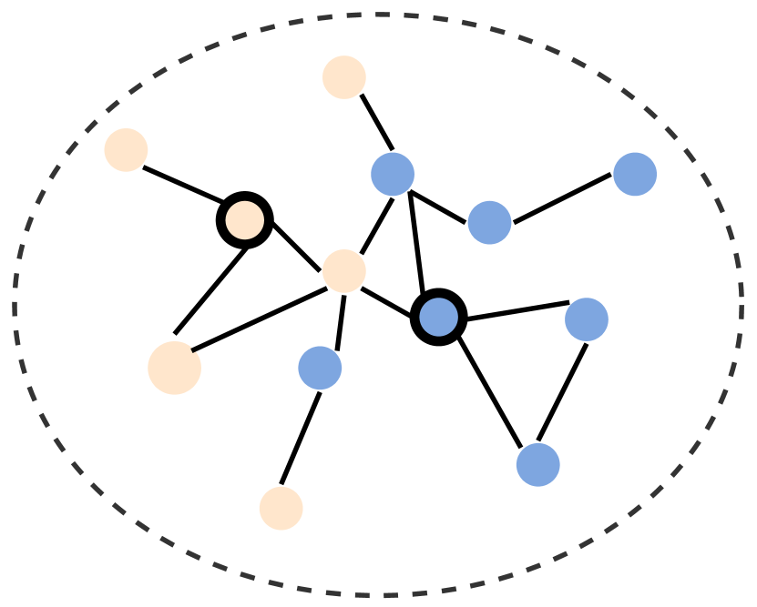
(a) Original Graph

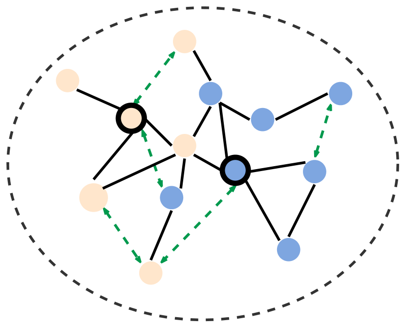
(b) Implicit Modelling

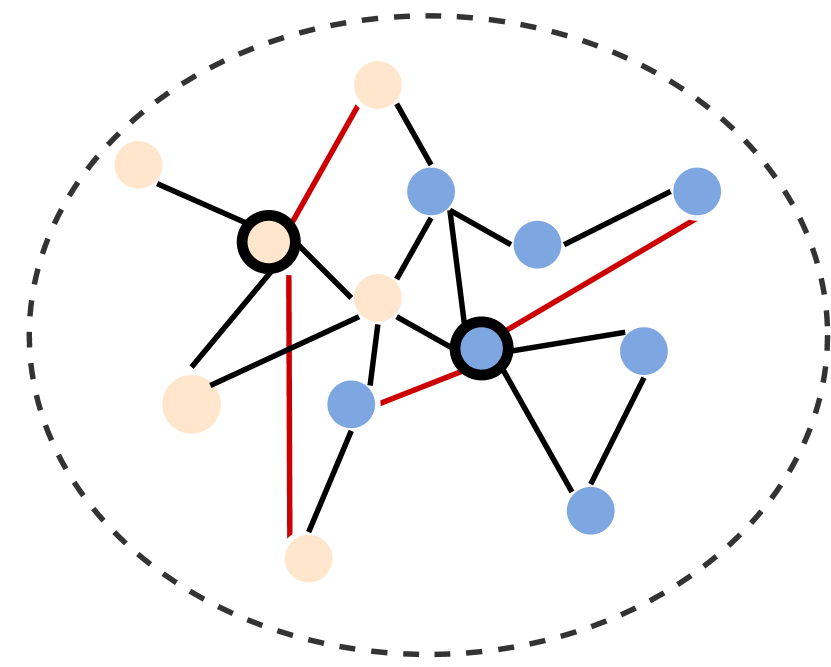
(c) Explicit Modelling

Figure 2: The schematic diagram for our solutions. Figure (a) displays a virtual graph with nodes in two categories (blue and yellow). Nodes with black border represent labeled nodes. From this figure, we can observe that some nodes are topologically far away from the labeled node, and these nodes are easy to be wrongly predicted according to Figure 1. Figure (b) shows our implicit solution to modelling the long-distance node relation, which implicitly models two nodes by learning their relation (the green dotted lines with arrows means predicting the node pair relation that whether two nodes are of the same category). Figure (c) shows our explicit solution, which directly adds edges between nodes of the same category (the red straight lines represent the added edges for reducing the distance to labeled node).

Graph neural networks (GNNs) have achieved promising results on semi-supervised node classification by learning node representations through information propagation along edges between nodes (Kipf and Welling, 2017; Hamilton et al., 2017; Bai et al., 2019; Verma et al., 2018; Li et al., 2016; Morris et al., 2019; Qu et al., 2019; Hu et al., 2019; Zhu et al., 2019; Verma et al., 2019). However, a typical GNN architecture has finite hops to propagate information along edges, which limits its capability of modelling the relation between nodes with long topological distance. We depict the problem in Figure 1 using GCN (Kipf and Welling, 2017) as an example. It shows that regardless of the layer number of GCN, the node classification accuracy of the three models all drops substantially as the topological distance from labeled nodes to unlabeled nodes increases (here the labeled node and the unlabeled node are of the same category; similarly hereinafter). Thus, modelling long-distance node relations is an essential and challenging problem for node representation learning and downstream tasks.

Current studies that aim to overcome limited hops in GNNs for information propagation focus on designing a deep GNN architecture (Li et al., 2019a; Rong et al., 2019; Zhao and Akoglu, 2019). Yet, deep GNNs face the over-smoothing issue (Li et al., 2018; Chen et al., 2020) that all node representations will become indistinguishable. More importantly, deep GNNs cannot fundamentally address the problem of modelling long-distance node relations, because the number of hops is still limited for information propagation due to the finite layer number of a deep GNN. Thus, it is infeasible for deep GNNs to model the relation between nodes in a particularly long topological distance.

To solve the problem of modelling long-distance node relations, we propose a new perspective by simply relying on shallow GNNs (i.e., a two-layer GNN). Specifically, we provide two solutions: (1) Implicitly modelling node relations by predicting whether two nodes are of the same category; (2) Explicitly modelling node relations by adding edges between two nodes that potentially have the same category label. An illustration of our two solutions is shown in Figure 2. Figure 2 (a) shows an original graph consisting of two node categories, and we can observe that some nodes are topologically far away from the labeled nodes, causing a high probability of incorrect prediction according to Figure 1. In Figure 2 (b), we implicitly model long-distance node relations by predicting whether two nodes are of the same category. The motivation for this solution is to pass the category information from other nodes to the remote nodes (remote nodes refer to the unlabeled nodes that have a long topological distance to the labeled node) by distinguishing whether they are of the same category. Besides, Figure 2 (c) shows the explicitly modelling solution, which directly builds the information channel between the remote unlabeled node and the corresponding labeled node by adding edges.

Both of the two solutions are able to model node relations regardless of the topological distance. Thus, the two solutions enable a GNN to learn better node representations, especially for remote nodes. However, there is a key challenge in the implementation of the two solutions: there is no label provided for nodes except for the training set in the semi-supervised node classification setting. Thus, it is infeasible to directly conduct the implicit or the explicit modelling. To address this issue, we propose a simple yet effective training framework named to implicitly and explicitly model long-distance node relations in an indirect way. For the implicit modelling, we sample node pairs from the training set to estimate long-distance node relations. For the explicit modelling, we adopt the self-training approach by adding edges based on prediction results.

Our is model-agnostic and can be applied to any variant of GNNs. Extensive experimental results show that our achieves consistent and significant improvements over four representative GNN models on three benchmark graph datasets (CORA, CiteSeer, PubMed) with limited extra computational cost. We also achieve state-of-the-art performance on CORA and CiteSeer. The main contributions of this work are as follows:

• For modelling long-distance node relations in graph structured data, we provide two solutions which simply rely on shallow GNNs: (1) Implicit modelling long-distance node relations by predicting the node pair relation, and (2) Explicit modelling long-distance node relations by adding edges between nodes that potentially have the same label.

• We design a model-agnostic framework named based on the implicit and explicit solutions, which overcomes the challenge of insufficient labeled nodes in the semi-supervised learning.

• Results show that our achieves consistent improvements over four representative GNNs on three benchmark graph datasets and state-of-the-art performance on CORA and CiteSeer, which verifies the effectiveness and the generalizability of our method.

2 Method

In this section, we will first introduce tasks for our method, and provide details of our based on the implicit and explicit solutions to modelling long-distance node relations.

2.1 Solution Formalization

For an undirected graph given the node feature matrix $\bm{X}\in\mathbb{R}^{n\times h}$ and the node adjacency matrix $\bm{A}\in\mathbb{R}^{n\times n}$ ($n$ denotes the node size of the graph and $h$ denotes the dimension size of the initial node embedding), the node classification task aims to train a classifier $f_{n}$ (usually a GNN model) to distinguish nodes of different categories:

$$\hat{\bm{l}}=f_{n}(\bm{X},\bm{A})$$ (1)

where $\hat{\bm{l}}\in\mathbb{R}^{n}$ is the predicted category label for all nodes. Different from the node classification task, we design a new task named as node pair classification to assist in training GNNs. The node pair classification task aims to train a different classifier $f_{p}$ to predict whether two nodes are of the same category:

$$\hat{\bm{r}}=f_{p}(\bm{X},\bm{A})$$ (2)

where $\hat{\bm{r}}\in\mathbb{R}^{n\times n}$ and $\hat{\bm{r}}_{i,j}\in\{0,1\}$ ($0$ means the $i$-the and $j$-th nodes are of different categories and $1$ denotes they are of the same category). Usually, the total number of all node pairs ($n\times n$) is too large to be enumerated, thus we need a sampling strategy $\mathrm{Sample}(\cdot)$ to sample some node pairs for loss calculation. For the prediction in Eq 1, 2, we calculate the training loss as:

$$\mathcal{L}_{node} =\mathrm{LossFunc_{1}}(\hat{\bm{l}},\bm{l})$$ (3)

$$\hat{\bm{r}}^{\prime} =\mathrm{Sample}(\hat{\bm{r}})$$ (4)

$$\mathcal{L}_{pair} =\mathrm{LossFunc_{2}}(\hat{\bm{r}}^{\prime},{\bm{r}^{\prime}})$$ (5)

$\mathrm{LossFunc_{1}}$ and $\mathrm{LossFunc_{2}}$ are the loss functions for the node and the node pair classification tasks, respectively. $\bm{l}$ is the gold label for the node classification task and $\bm{r}^{\prime}$ is the gold label of sampled node pairs for the node pair classification task. According to Figure 2 (b), node pair prediction enables to model relations between any node pairs, which transfers the category information between nodes. Therefore, we propose to predict the node category label and the node pair relation in a single model, and combine $\mathcal{L}_{pair}$ and $\mathcal{L}_{node}$ to form the loss function as:

$$\mathcal{L}=\mathcal{L}_{node}+\lambda\cdot\mathcal{L}_{pair}$$ (6)

where $\lambda$ is the parameter to control the influence of the node pair classification task. When $\lambda=0$, it falls back to conventional GNN training.

1:A GNN:${g}(\bm{X},\bm{A})$. Node feature matrix $\bm{X}$. Adjacency Matrix $\bm{A}$. Number of epochs $N$. Number of max iteration time $max_{t}$. Gold label for node and node pair $\bm{Y,P}$. Loss functions for node and node pair$\mathcal{L}_{1},\mathcal{L}_{2}$. Node pair loss weight $\lambda$. Mask matrix $\mathbf{Mask}$.

2:$\mathrm{valid\_acc_{0}}=0$

3:for iter times $\mathrm{i}\in[1,max_{t}]$ do

4:     for $t\in[1,N]$ do

5:         $\mathbf{l}$, $\mathbf{r}$ = ${g_{i}}(\bm{X},\bm{A})$ $\triangleright$ Predict node category label and node pair relation jointly

6:         $\mathcal{L}_{node}=\mathcal{L}_{1}\big{(}\mathbf{l}_{[train]},\bm{Y}_{[train]}\big{)}$

7:         $\mathcal{L}_{pair}=\mathcal{L}_{2}\big{(}\mathbf{r}_{[pair]},\bm{P}_{[pair]}\big{)}$

8:         $\mathcal{L}=\mathcal{L}_{node}+\mathcal{\lambda}*\mathcal{L}_{pair}$

9:         Back propagate $\mathcal{L}$

10:     end for

11:     $\mathrm{valid\_acc_{i}}\leftarrow\mathrm{Accuracy}(\mathbf{l}_{[valid]},\bm{Y}_{[valid]})$

12:     if $\mathrm{valid\_acc_{i}}\leq\mathrm{valid\_acc_{i-1}}$ then

13:         $\mathrm{test\_acc_{i}}\leftarrow\mathrm{Accuracy}(\mathbf{l}_{[test]},\bm{Y}_{[test]})$

14:         $\mathbf{return\,}\mathrm{test\_acc_{i}}$

15:     end if

16:     $\bm{R}^{n}\leftarrow\mathbf{l\times l}$

17:     $\bm{R}^{p}\leftarrow\mathbf{r}$

18:     $\bm{R}\leftarrow\bm{R}^{n}\wedge\bm{R}^{p}$ $\triangleright$ Obtain prediction matrix for adding edges by the joint decision of node and node pair prediction.

19:     $\bm{R}^{\prime}\leftarrow\bm{R}\circ\mathbf{Mask}$ $\triangleright$ Select position for edge addition

20:     $\bm{A}\leftarrow\bm{A}\vee\bm{R}^{\prime}$

21:end for

22:$\mathrm{test\_acc_{i}}\leftarrow\mathrm{Accuracy}(\mathbf{l}_{[test]},\bm{Y}_{[test]})$

23:$\mathbf{return\,}\mathrm{test\_acc_{i}}$

Algorithm 1 HighwayGraph

2.2

To combine the implicit solution and the explicit solution, we propose for training GNNs. The full algorithm of is presented in Algorithm 1. A key challenge for implementing the implicit and the explicit solution is that there is no label provided for nodes except for the training set in the semi-supervised learning. Thus, is a self-training approach with multiple iterations. During one training iteration, learns the node and node pair classification jointly (the node pairs are extracted from the training set). Then we optimize the original graph topology by adding edges between intra-category nodes according to the joint decision of node and node pair prediction results. We then train the next iteration based on the optimized graph topology. The following sections will elaborate the implicit and explicit ways of modelling long-distance node relations in .

2.2.1 Implicit Modelling: Co-training with Node Pair Classfication

Given the node embedding $\bm{X}$, the adjacency matrix $\bm{A}$ (either an original graph or an optimized graph), and a GNN model ${\rm GNN_{\alpha}}$, we first get hidden representations of nodes:

$$\bm{y} ={\rm GNN_{\alpha}}(\bm{X},\bm{A})$$ (7)

Then we predict the node category label and the node pair relation based on $\bm{y}$:

$$\hat{\bm{l}} ={\rm softmax}(\bm{y})$$ (8)

$$\hat{\bm{r}} ={\rm sigmoid}(\bm{y}\cdot\bm{y}^{\top})$$ (9)

where $\hat{\bm{l}}\in\mathbb{R}^{n}$ is the predicted node category label and $\hat{\bm{r}}\in\mathbb{R}^{n\times n}$ is the predicted node pair relation. $n$ denotes the node size of the graph. $\hat{\bm{r}}_{i,j}\in[0,1]$ represents the relation between the $i$-th node and the $j$-th node: when $\hat{\bm{r}}_{i,j}$ is close to 1, two nodes are more likely to be of the same category, and vice versa.

The sampling strategy (introduced in Eq 4) used in is sampling all the node pairs in the training set, which are the only available labeled nodes during the training. The size of the training set is usually limited in the semi-supervised learning, thus we keep all the node pairs in the training set. As introduced in Eq 3, 5, we calculate the Negative Log Loss ($\mathrm{LossFunc_{1}}$) and the Binary Cross Entropy Loss ($\mathrm{LossFunc_{2}}$) for node label and node pair relation predictions, respectively:

$$\mathcal{L}_{node}= -\sum^{T}_{i=1}\bm{l}_{i}\,\log\,p(\,\hat{\bm{l}}_{i})$$ (10)

$$\begin{split}\mathcal{L}_{pair}=&-\sum^{T}_{i=1}\sum^{T}_{j=1}\{\bm{r}_{i,j}\cdot{\rm log}(\hat{\bm{r}}_{i,j})\\ &+(1-\bm{r}_{i,j})\cdot{\rm log}(1-\hat{\bm{r}}_{i,j})\}\end{split}$$ (11)

where $T$ is the size of the training set; $\bm{l}$ and $\bm{r}$ are the gold labels for the node category and the node pair relation, respectively; $\bm{r}$ is extracted from $\bm{l}$ by identifying whether two nodes are of the same category. The final training loss is defined in Eq. 6.

In experiments, we also use different GNN architectures to co-train the two tasks, such as leveraging two different GNN layers after sharing the same first layer, or adding a trainable parameter matrix in Eq 9. However, these techniques lead to performance degradation and extra training cost.

2.2.2 Explicit Modelling: Adding Intra-category Edges

Besides the implicit solution by co-training with node pair classification, we also adopt an explicit way to model long-distance node relations in by adding edges between nodes of the same category. Since most node labels are not available in the semi-supervised training, we use the self-training method and add edges based on the joint decision of node classification and node pair classification prediction results. For node label prediction in Eq 8, we get the node label prediction matrix $\bm{R}^{n}$ by considering the predicted labels and the confidence of two nodes:

$$\bm{R}^{n}_{i,j}=\begin{cases}1,&\hat{\bm{l}}_{i}=\hat{\bm{l}}_{j},\bm{c}_{i}>t_{n},\bm{c}_{j}>t_{n}\\ 0,&{\rm otherwise}\end{cases}$$ (12)

where $\bm{c}_{i}$ is the prediction confidence for the $i$-th node (the max value of tensor after softmax operation in Eq 8). $t_{n}\in[0,1]$ is the confidence threshold to filter out low-confidence predictions. For node pair relation prediction in Eq 9, we get the node pair prediction matrix $\bm{R}^{p}$ calculated with a threshold $t_{p}\in[0,1]$:

$$\bm{R}^{p}_{i,j}=\begin{cases}1,&\hat{\bm{r}}_{i,j}\geq t_{p}\\ 0,&\hat{\bm{r}}_{i,j}<t_{p}\end{cases}$$ (13)

Then we combine $\bm{R}^{n}$ and $\bm{R}^{p}$ to make a joint decision and access a more reliable prediction matrix for explicitly modelling long-distance node relations. We conduct element-wise ${\rm AND\;(\wedge)}$ operation to access the prediction matrix for adding intra-category edges:

$$\bm{R} =\bm{R}^{n}\wedge\bm{R}^{p}$$ (14)

$$\bm{R}^{\prime} =\bm{R}\circ\mathbf{Mask}$$ (15)

$$\bm{A}^{\prime} =\bm{A}\vee\bm{R}^{\prime}$$ (16)

$\vee$ is the element-wise ${\rm OR}$ operation, $\circ$ is the element-wise multiplication operation, $\bm{A}$ is the original adjacency matrix, and $\bm{A}^{\prime}$ is the updated adjacency matrix used in the next training iteration. $\mathbf{Mask}$ is a mask matrix to select the position to add edges.

In the explicit modeling method, we propose to reduce the long topological distance by adding edges between remote nodes and labeled nodes, so we filter out several rows of $\bm{R}$ to add edges by setting the values of these rows in $\mathbf{Mask}$ to be $1$ and all other values be $0$. In practice, we select one row per category from the training set (i.e. there are 7 categories in CORA dataset, and we select 7 nodes with different labels from the training set and then select the rows corresponding to these 7 nodes from $\bm{R}$). We find that adding too many edges may cause performance decline. One possible reason is that adding too many edges may introduce too much noise (wrongly added edges) which misleads the node representation learning process.

Acc (%)	CORA				PubMed				CiteSeer
Model	GCN	GAT	SAGE	Hyper	GCN	GAT	SAGE	Hyper	GCN	GAT	SAGE	Hyper
Typical GNN Training	80.1$\pm$2.0	78.5$\pm$1.0	80.1$\pm$1.0	79.9$\pm$1.0	76.5$\pm$1.3	75.0$\pm$1.0	75.3$\pm$1.6	73.6$\pm$1.5	67.0$\pm$0.7	66.7$\pm$1.0	66.6$\pm$1.0	64.3$\pm$0.8
(Full Method)	83.2$\pm$0.8	83.4$\pm$0.6	84.2$\pm$0.7	83.0$\pm$1.0	77.2$\pm$0.5	76.1$\pm$1.5	75.9$\pm$1.8	74.5$\pm$1.3	70.2$\pm$0.4	68.5$\pm$0.3	68.7$\pm$0.5	67.1$\pm$0.3
(w/o Joint Deci.)	82.6$\pm$1.1	82.7$\pm$0.8	83.6$\pm$0.7	82.3$\pm$1.0	77.1$\pm$0.6	76.1$\pm$1.6	75.6$\pm$1.8	74.2$\pm$1.5	69.3$\pm$0.4	68.3$\pm$0.6	68.2$\pm$0.7	66.0$\pm$0.9
(w/o Explicit Link)	83.0$\pm$1.0	81.5$\pm$1.1	82.7$\pm$1.0	81.0$\pm$0.8	76.9$\pm$1.3	75.6$\pm$1.2	75.1$\pm$1.8	74.1$\pm$1.5	68.0$\pm$0.6	67.8$\pm$0.9	67.8$\pm$0.9	64.9$\pm$0.9

Table 1: Node classification results (% test accuracy) compared to the baselines across three benchmark datasets using four representative GNN models with random dataset splitting. The mean accuracy and the standard deviation of each experiment are calculated after 15 running times (5 random dataset splitting and 3 random initial seeds for each splitting). Experiments in the same column adopt the same GNN model and set the same hyper-parameters for comparison. We can find that our brings significant and consistent performance improvements for all the graph datasets and models.

3 Experiments

3.1 Datasets and Models

We evaluate our proposed on three benchmark graph datasets: CORA, CiteSeer and PubMed (Sen et al., 2008). These datasets are citation graph networks, which have been widely used to evaluate GNNs  (Maehara, 2019; Li et al., 2018; Bianchi et al., 2019; Fey, 2019). To verify the generalizability of , we select four representative GNN architectures as the experimental models:

• GCN (Graph Convolutional Network) (Kipf and Welling, 2017) which uses the spectral method to conduct convolution operation.

• GAT (Graph Attention Network) (Veličković et al., 2018) which adopts the attention mechanism to aggregate neighborhood node information.

• SAGE (GraphSAGE) (Hamilton et al., 2017) which uses a sampling method to propagate information in large graphs.

• Hyper (HyperGraph) (Bai et al., 2019) which utilizes the high-order information of graphs.

3.2 Experimental Settings

Following Shchur et al. (2018); Sun et al. (2019), we run $5$ random dataset splittings using the 20/30/rest splitting method, and use $3$ random initial seeds for each splitting method in each experiment to reduce the randomness of the results caused by dataset splittings and initial seeds. The mean accuracy and standard deviation of each experiment for $15$ runs are reported. To achieve a highly reliable confidence of graph topology optimization, we set the category threshold of the node pair classification to a rather high value (i.e. $0.9$), which aims to achieve a high-precision and low-recall classifier for two nodes of the same category (there is no need to add all the intra-category edges, but the precision of added edges need to be guaranteed). The implementation of the GNN models is based on PyTorch (Paszke et al., 2017) and PyTorch Geometric (Fey and Lenssen, 2019), without changing the implementation of the convolutional layer and dataset in PyTorch Geometric. Hyperparameters of each GNN are tuned in each group (experiments using the same GNN model on the same graph dataset). Then all the hyperparameters (including the splitting seeds and the initial seeds) are fixed in each experiment group for fair comparison. For the node pair classification, we increase the weight of positive samples, since the negative samples are far more than the positive samples.

For all the experimental models, we use full-batch training with a maximum number of training epochs $200$. We use early stopping and stop optimization if the validation accuracy is no longer increased in $10$ epochs. We use dropout (Hinton et al., 2012) method to avoid over-fitting and the dropout rate is tuned in $\{0.3,0.4,0.5,0.6,0.7\}$ for different combinations of the GNN models and the graph datasets. The hidden layer number of each GNN model is set to $2$, which can achieve the best performance for GNNs. The hidden size of each hidden layer is tuned in $\{32,64,128,256\}$. We use Adam (Kingma and Ba, 2015) as the optimizer; the initial learning rate is selected in $\{5\times 10^{-4},1\times 10^{-3},2\times 10^{-3},3\times 10^{-3}\}$.

3.3 Baselines

We compare our proposed training framework with the typical GNN training method, as well as two ablation versions of

• Typical GNN Training: GNNs are trained on the original graph topology using standard semi-supervised training framework (Yang et al., 2016).

• (w/o Joint Decision): This ablation version adds edges only based on node label predictions, which is designed to evaluate the effects of co-training with node pair classification.

• (w/o Explicit modelling): Another ablation version of which only conducts the first-turn training and does not retrain on the updated graph. This baseline is designed to evaluate the effects of both co-training and iterative training operations.

4 Results and Analysis

4.1 Overall Results

The performance of our method and other baselines are shown in Table 1. From the results, we can observe that:

(1) Combining both the implicit modelling (co-training with node pair classification) and the explicit modelling (adding edges), our proposed especially improves the performance of the typical GNN training method by a large margin among all the four experimental GNNs. The results demonstrate both the effectiveness and the generalizability of .

(2) Our performs well on the GraphSAGE architecture, which is designed for large-scale graph networks. Thus, our method shows great potential for applications involving large graphs.

(3) The (w/o Explicit Link) method outperforms all the GNNs trained using the typical method, which validates the effect of co-training with node pair classification.

(4) Removements of the explicit linking and the joint-decision mechanism both cause significant performance degradation, which demonstrates the effectiveness of the two methods in our .

Method	CORA		PubMed		CiteSeer
GCN* (Kipf and Welling, 2017)	81.5		79.0		70.3
GAT* (Veličković et al., 2018)	83.0		79.0		72.5
GMNN* (Qu et al., 2019)	83.7		81.8		73.1
Trun. Krylov* (Luan et al., 2019)	83.8		80.1		74.2
GraphMIX* (Verma et al., 2019)	83.9		81.0		74.5
G-APPNP* (Zhu et al., 2019)	84.3		81.0		72.0
Graph U-net* (Gao and Ji, 2019)	84.4		79.6		73.2
H-GCN* (Hu et al., 2019)	84.5		79.8		72.8
(Ours)	85.7	$\pm$ 0.5	80.1	$\pm$0.4	75.1	$\pm$0.2

Table 2: Node classification results in comparison with recent state-of-the-art methods with standard dataset splitting Yang et al. (2016). We run 10 turns for each experiment and report the mean value and the standard deviation over the running times. [*] means the results are taken from the corresponding papers. Our set the new SOTA for the CORA and CiteSeer datasets.

(a) GCN, $\lambda$ = 0

(b) GCN, $\lambda$ = 0.5

(c) GCN, $\lambda$ = $1.0$

Figure 3: 2D visualization (t-SNE) of the nodes distribution in CORA graph. Nodes of the same category share the same color. We display the node representations of the second layer in the 2-layer GCN model using our framework under different loss weight $\lambda$ of node pair prediction from Eq 6. We can easily find that with the increase of $\lambda$, nodes of the same category are more concentrated and nodes of different classes are more separated. The prediction accuracy is also increased.

(a) GCN

(b) GAT

(c) HYPER

(d) SAGE

Figure 4: The accuracy values of nodes sets with different hops to the labeled node. We display the result of all the four experiment models with different node pair loss weights ($0$/$0.5$/$1.0$). We can obviously find that for all models, adding node pair loss can help predict long-distance nodes better.

4.2 Comparison with State-of-the-art

In this subsection, we display the comparison results between our and state-of-the-art node classification methods in the setting of standard Planetoid (Yang et al., 2016) dataset splitting for CORA/CiteSeer/PubMed datasets. The base model used for framework is GCN or GraphMix (Verma et al., 2019). For baselines, we choose classical GCN and GAT and some recent advanced methods. The results are shown in Table 2. We can observe that our outperforms all the baselines and achieves state-of-the-art performance on CORA and CiteSeer. Our approach also shows competitive results on PubMed. The limited improvements on PubMed is because that there are only few labeled nodes (60) in the training set that provide inadequate supervision information for the node pair classification task (node pairs of the same category constitute a small part of all the node pairs, so there are few positive samples).

4.3 Effects of Co-training

To examine the effects of node pair classification, we display 2D visualization of the node distribution belonging to different categories with varying loss weight $\lambda$ for node pair classification in Figure 3. We train a 2-layer GNN and use T-SNE (Rauber et al., 2016) to reduce hidden states to two dimensions. From Figure 3, we can observe that with the increase of $\lambda$, nodes of the same category are more concentrated and nodes of different categories are more separated, which makes GCN easier to set node classification boundaries with fewer prediction errors. Besides, with the increase of $\lambda$, the node classification accuracy can be generally improved. Thus, co-training with node pair classification indeed facilitates GCN training and enables to achieve higher accuracy. We observe similar phenomena in other GNNs, but we only display the node distribution for GCN due to limited space.

4.4 Results of the Long-distance Nodes

Our is designed to model long-distance node relations. To verify the effectiveness of in modeling long-distance node relations, we split the test set into different subsets according to the topological distance between unlabeled nodes and labeled nodes, and present prediction results of each subset. Results of the four experiment GNNs are displayed in Figure 4. We can observe that for all the GNNs, adding node pair loss can help predict long-distance nodes better, which verifies the effectiveness of in modeling long-distance node relations.

Acc (%)	$\lambda$=0	$\lambda$=0.5	$\lambda$=1.0	$\lambda$=2.0
10 Nodes	78.5	78.8	79.3	78.5
20 Nodes	78.6	80.8	82.5	82.8
30 Nodes	80.6	84.2	84.6	84.8
40 Nodes	83.1	85.8	86.4	86.3
50 Nodes	83.5	86.4	86.3	86.8

Table 3: Accuracy values (GCN model on the CORA dataset) of different node pair loss weight (x-axis) under different labeled node size per class (y-axis). We can find that our can achieve consistent improvement with different training set size.

Acc (%)	Lead	Random	Close	Middle	Remote
100k	85.9	86.3	84.5	85.6	85.9
200k	86.2	86.4	85.6	86.0	86.5
300k	86.2	86.7	85.4	85.7	86.6
400k	86.9	87.2	85.8	85.7	86.5
500k	86.4	86.0	85.6	85.4	86.9

Table 4: Accuracy values (GCN model on the CORA dataset; 50 labeled nodes per category) of different sampling strategy (x-axis) under different sampling size (y-axis). “Lead” denotes sampling the front node pairs; “Random” means randomly sampling; “Close”, “Middle”, “Remote” denote sampling the node pairs with a higher probability for the node pairs with close, middle and remote topological distance, respectively. We can find that the “Random” strategy and the “Remote” strategy perform best among all strategies under different sampling numbers.

4.5 Analysis of Node Pair Sampling

Limited by the accessible nodes labels, our takes the node pairs from the training set for training. In this subsection, we conduct some extended analyses for the sampling process. Firstly, in Table 3, we present the results of GCN with different node pair loss weight $\lambda$ and labeled node size per class. We can find that our can achieve consistent improvement with different training set size. Secondly, in Table 4, we change sampling strategies under different total numbers of sampled node pairs. We set the labeled node size per class to be 50, so that we can design different sampling methods. The results show that the Random strategy and the Remote strategy perform best in different sampling numbers. We can also conclude that modelling the node pair relations for the remote nodes are more effective than modelling close nodes, because the long-distance relations are hardly learned by the original GNN models.

5 Related Work

The semi-supervised learning framework has been widely used on the node classification task (Kipf and Welling, 2017; Hamilton et al., 2017; Defferrard et al., 2016). Recent works have proposed new advanced training methods. For example, Xu et al. (2018) propose jumping knowledge networks to utilize information from high-order neighbors. (Verma et al., 2019) propose to apply the manifold mixup in GNN training to generate some virtual samples. Rong et al. (2019) propose to remove edges randomly at each epoch and acts as a data augmenter or a message passing reducer.

Modeling long-distance relations is vital for GNN training and applications. Recent studies (Li et al., 2019a; Rong et al., 2019; Zhao and Akoglu, 2019) try to build deep GNN architectures or use the hyper-graph information (Fey, 2019; Bai et al., 2019; Jiang et al., 2019b). However, these solutions can hardly model the very long-distance node relations. Instead, our HighwayGraph framework can model the node relations regardless of their topological distance by simply relying on shallow GNN models.

Different GNN architectures (Bianchi et al., 2019; Verma et al., 2018; Li et al., 2019b) have been designed for graph-related tasks with different motivations. Most existing works directly use the original graph topology, while Chen et al. (2020) prove that the performance of GNNs can be improved by graph topology optimization. Other works also refer to the dynamic graphs. Zhou et al. (2019) propose the EvolveGCN model by using the RNN model to update GCN. Yang et al. (2019) propose to train GCN and refine the graph topology at the same time. Some other works (Jiang et al., 2019a; Franceschi et al., 2019) also try to learn and update the graph topology. Different from these works, our method optimizes graph with a clear target to build the information highway especially for remote nodes.

Self-training is a popular framework in the semi-supervised task as it can extend the supervised information based on prediction results. Li et al. (2018) propose to use predicted pseudo labels as the supervision information for the next training iteration. Zhou et al. (2019); Stretcu et al. (2019) follow and update this idea. Different from the method of using pseudo labels, our proposed HighwayGraph takes the advantage of predicted pseudo edges, which has proven significant performance improvements over multiple GNN models across benchmark graph datasets.

6 Conclusion

We propose to model long-distance node relations for graph structured data by simply relying on shallow GNNs. We provide two solutions: (1) Implicitly modelling node pairs by predicting their relations, and (2) Explicitly modelling node relations by adding edges. Then we introduce a novel GNN training framework named to combine these two solutions. Extensive experimental results demonstrate that our proposed consistently and significantly achieves improvements over multiple GNNs on three benchmark graph datasets with limited extra computational cost, which verifies the effectiveness and generalization of our method. Besides, enables to significantly improve prediction accuracy for unlabeled nodes that are far away from labeled nodes, which further justifies the two proposed solutions to modelling long-distance node relations. In the future, we plan to find better methods in this direction.

7 Acknowledgements

This work was supported in part by a Tencent Research Grant. Xu Sun is the corresponding author of this paper.

Appendix A Additional Computational Cost of

Compared to the standard semi-supervised node classification, the module of graph topology optimization and the module of co-training in our framework will cause inevitable additional computational cost. However, the additional computational cost is limited.

(1) Graph Optimization Cost

In experiments, we observe that a well-optimized graph topology is effective for consistently improving the performance of multiple GNNs on the same graph dataset, so our can be easily transferred among different GNN models without extra computational cost for the graph topology optimization.

(2) Co-training Cost

Eq 9 is presented for a better understanding and can be optimized in practice. When training the node pair classification task, the supervision information is accessed from the training set of the node classification task, which is very small in the semi-supervised framework (20 nodes from each category as the training set; the whole training set usually has 60-200 nodes). Thus the size of training node pairs for the node pair classification task is also limited. When computing the training loss, we access the training set nodes first and then conduct matrix multiply in Eq 9, thus the computational complexity is $O(m\cdot m)$ instead of $O(n\cdot n)$ ($m$ denotes the training size and $n$ denotes the node size; usually $m\ll n$). Besides, in the co-training module, the prediction of the node pair relation requires no extra trainable parameters and causes only a small increase in GPU memory occupancy.

References

- Bai et al. (2019) Song Bai, Feihu Zhang, and Philip HS Torr. 2019. Hypergraph Convolution and Hypergraph Attention. arXiv preprint arXiv:1901.08150.
- Bianchi et al. (2019) Filippo Maria Bianchi, Daniele Grattarola, Lorenzo Livi, and Cesare Alippi. 2019. Graph Neural Networks with Convolutional Arma Filters. arXiv preprint arXiv:1901.01343.
- Chen et al. (2020) Deli Chen, Yankai Lin, Wei Li, Peng Li, Jie Zhou, and Xu Sun. 2020. Measuring and Relieving the Over-smoothing Problem for Graph Neural Networks from the Topological View. In Proceedings of the AAAI Conference on Artificial Intelligence, AAAI 2020.
- Defferrard et al. (2016) Michaël Defferrard, Xavier Bresson, and Pierre Vandergheynst. 2016. Convolutional Neural Networks on Graphs with Fast Localized Spectral Filtering. In Advances in Neural Information Processing Systems, pages 3837–3845.
- Fey (2019) Matthias Fey. 2019. Just Jump: Dynamic Neighborhood Aggregation in Graph Neural Networks. arXiv preprint arXiv:1904.04849.
- Fey and Lenssen (2019) Matthias Fey and Jan E. Lenssen. 2019. Fast Graph Representation Learning with PyTorch Geometric. In ICLR Workshop on Representation Learning on Graphs and Manifolds.
- Franceschi et al. (2019) Luca Franceschi, Mathias Niepert, Massimiliano Pontil, and Xiao He. 2019. Learning Discrete Structures for Graph Neural Networks. In Proceedings of the 36th International Conference on Machine Learning, ICML 2019, 9-15 June 2019, Long Beach, California, USA, volume 97 of Proceedings of Machine Learning Research, pages 1972–1982. PMLR.
- Gao and Ji (2019) Hongyang Gao and Shuiwang Ji. 2019. Graph U-Nets. In Proceedings of the 36th International Conference on Machine Learning, ICML 2019, pages 2083–2092.
- Hamilton et al. (2017) William L. Hamilton, Zhitao Ying, and Jure Leskovec. 2017. Inductive Representation Learning on Large Graphs. In Advances in Neural Information Processing Systems, pages 1024–1034.
- Hinton et al. (2012) Geoffrey E. Hinton, Nitish Srivastava, Alex Krizhevsky, Ilya Sutskever, and Ruslan Salakhutdinov. 2012. Improving neural networks by preventing co-adaptation of feature detectors. CoRR, abs/1207.0580.
- Hu et al. (2019) Fenyu Hu, Yanqiao Zhu, Shu Wu, Liang Wang, and Tieniu Tan. 2019. Hierarchical Graph Convolutional Networks for Semi-supervised Node Classification. In Proceedings of the Twenty-Eighth International Joint Conference on Artificial Intelligence, IJCAI 2019, pages 4532–4539.
- Jiang et al. (2019a) Bo Jiang, Ziyan Zhang, Doudou Lin, Jin Tang, and Bin Luo. 2019a. Semi-supervised learning with graph learning-convolutional networks. In IEEE Conference on Computer Vision and Pattern Recognition, CVPR 2019, Long Beach, CA, USA, June 16-20, 2019, pages 11313–11320. Computer Vision Foundation / IEEE.
- Jiang et al. (2019b) Jianwen Jiang, Yuxuan Wei, Yifan Feng, Jingxuan Cao, and Yue Gao. 2019b. Dynamic hypergraph neural networks. In Proceedings of the Twenty-Eighth International Joint Conference on Artificial Intelligence, IJCAI 2019, pages 2635–2641.
- Kingma and Ba (2015) Diederik P. Kingma and Jimmy Ba. 2015. Adam: A Method for Stochastic Optimization. In 3rd International Conference on Learning Representations, ICLR 2015, San Diego, CA, USA, May 7-9, 2015, Conference Track Proceedings.
- Kipf and Welling (2017) Thomas N Kipf and Max Welling. 2017. Semi-supervised Classification with Graph Convolutional Networks. In 5th International Conference on Learning Representations, ICLR 2017.
- Li et al. (2019a) Guohao Li, Matthias Muller, Ali Thabet, and Bernard Ghanem. 2019a. DeepGCNs: Can GCNs go as deep as CNNs? In Proceedings of the IEEE International Conference on Computer Vision, pages 9267–9276.
- Li et al. (2018) Qimai Li, Zhichao Han, and Xiao-Ming Wu. 2018. Deeper Insights into Graph Convolutional Networks for Semi-supervised Learning. In Thirty-Second AAAI Conference on Artificial Intelligence.
- Li et al. (2019b) Wei Li, Jingjing Xu, Yancheng He, Shengli Yan, Yunfang Wu, and Xu Sun. 2019b. Coherent Comments Generation for Chinese Articles with a Graph-to-Sequence Model. In ACL 2019, Florence, Italy, July 28- August 2, 2019, pages 4843–4852.
- Li et al. (2016) Yujia Li, Daniel Tarlow, Marc Brockschmidt, and Richard S. Zemel. 2016. Gated Graph Sequence Neural Networks. In 4th International Conference on Learning Representations, ICLR 2016.
- Luan et al. (2019) Sitao Luan, Mingde Zhao, Xiao-Wen Chang, and Doina Precup. 2019. Break the Ceiling: Stronger Multi-scale Deep Graph Convolutional Networks. In Advances in Neural Information Processing Systems 32: Annual Conference on Neural Information Processing Systems 2019, NeurIPS 2019, 8-14 December 2019, Vancouver, BC, Canada, pages 10943–10953.
- Maehara (2019) Takanori Maehara. 2019. Revisiting graph neural networks: All we have is low-pass filters. arXiv preprint arXiv:1905.09550.
- Morris et al. (2019) Christopher Morris, Martin Ritzert, Matthias Fey, William L Hamilton, Jan Eric Lenssen, Gaurav Rattan, and Martin Grohe. 2019. Weisfeiler and Leman go Neural: Higher-order Graph Neural Networks. In Proceedings of the AAAI Conference on Artificial Intelligence, volume 33, pages 4602–4609.
- Paszke et al. (2017) Adam Paszke, Sam Gross, Soumith Chintala, Gregory Chanan, Edward Yang, Zachary DeVito, Zeming Lin, Alban Desmaison, Luca Antiga, and Adam Lerer. 2017. Automatic differentiation in PyTorch. In NIPS-W.
- Qu et al. (2019) Meng Qu, Yoshua Bengio, and Jian Tang. 2019. GMNN: graph markov neural networks. In Proceedings of the 36th International Conference on Machine Learning, ICML 2019, pages 5241–5250.
- Rauber et al. (2016) Paulo E. Rauber, Alexandre X. Falcão, and Alexandru C. Telea. 2016. Visualizing Time-Dependent Data Using Dynamic t-SNE. In Eurographics Conference on Visualization, EuroVis 2016, pages 73–77.
- Rong et al. (2019) Yu Rong, Wenbing Huang, Tingyang Xu, and Junzhou Huang. 2019. The Truly Deep Graph Convolutional Networks for Node Classification. arXiv preprint arXiv:1907.10903.
- Sen et al. (2008) Prithviraj Sen, Galileo Namata, Mustafa Bilgic, Lise Getoor, Brian Galligher, and Tina Eliassi-Rad. 2008. Collective classification in network data. AI magazine, 29(3):93–93.
- Shchur et al. (2018) Oleksandr Shchur, Maximilian Mumme, Aleksandar Bojchevski, and Stephan Günnemann. 2018. Pitfalls of Graph Neural Network Evaluation. arXiv preprint arXiv:1811.05868.
- Stretcu et al. (2019) Otilia Stretcu, Krishnamurthy Viswanathan, Dana Movshovitz-Attias, Emmanouil A. Platanios, Sujith Ravi, and Andrew Tomkins. 2019. Graph agreement models for semi-supervised learning. In Advances in Neural Information Processing Systems 32: Annual Conference on Neural Information Processing Systems 2019, NeurIPS 2019, 8-14 December 2019, Vancouver, BC, Canada, pages 8710–8720.
- Sun et al. (2019) Ke Sun, Piotr Koniusz, and Jeff Wang. 2019. Fisher-Bures Adversary Graph Convolutional Networks. In Proceedings of the Thirty-Fifth Conference on Uncertainty in Artificial Intelligence, page 161.
- Veličković et al. (2018) Petar Veličković, Guillem Cucurull, Arantxa Casanova, Adriana Romero, Pietro Lio, and Yoshua Bengio. 2018. Graph Attention Networks. In 6th International Conference on Learning Representations, ICLR 2018.
- Verma et al. (2018) Nitika Verma, Edmond Boyer, and Jakob Verbeek. 2018. Feastnet: Feature-steered Graph Convolutions for 3d Shape Analysis. In Proceedings of the IEEE Conference on Computer Vision and Pattern Recognition, pages 2598–2606.
- Verma et al. (2019) Vikas Verma, Meng Qu, Alex Lamb, Yoshua Bengio, Juho Kannala, and Jian Tang. 2019. GraphMix: Regularized Training of Graph Neural Networks for Semi-Supervised Learning. CoRR, abs/1909.11715.
- Wu et al. (2019) Qitian Wu, Hengrui Zhang, Xiaofeng Gao, Peng He, Paul Weng, Han Gao, and Guihai Chen. 2019. Dual Graph Attention Networks for Deep Latent Representation of Multifaceted Social Effects in Recommender Systems. In The World Wide Web Conference, WWW 2019, pages 2091–2102.
- Wu et al. (2018) Zhenqin Wu, Bharath Ramsundar, Evan N Feinberg, Joseph Gomes, Caleb Geniesse, Aneesh S Pappu, Karl Leswing, and Vijay Pande. 2018. MoleculeNet: a Benchmark for Molecular Machine Learning. Chemical science, 9(2):513–530.
- Wu et al. (2015) Zhirong Wu, Shuran Song, Aditya Khosla, Fisher Yu, Linguang Zhang, Xiaoou Tang, and Jianxiong Xiao. 2015. 3D ShapeNets: A deep representation for volumetric shapes. In IEEE Conference on Computer Vision and Pattern Recognition, CVPR 2015, pages 1912–1920.
- Xu et al. (2018) Keyulu Xu, Chengtao Li, Yonglong Tian, Tomohiro Sonobe, Ken-ichi Kawarabayashi, and Stefanie Jegelka. 2018. Representation learning on graphs with jumping knowledge networks. In Proceedings of the 35th International Conference on Machine Learning, ICML 2018, pages 5449–5458.
- Yang et al. (2019) Liang Yang, Zesheng Kang, Xiaochun Cao, Di Jin, Bo Yang, and Yuanfang Guo. 2019. Topology Optimization based Graph Convolutional Network. In Proceedings of the Twenty-Eighth International Joint Conference on Artificial Intelligence, IJCAI 2019, pages 4054–4061.
- Yang et al. (2016) Zhilin Yang, William W Cohen, and Ruslan Salakhutdinov. 2016. Revisiting Semi-supervised Learning with Graph Embeddings. In Proceedings of the 33nd International Conference on Machine Learning,ICML 2016, pages 40–48.
- Yi et al. (2016) Li Yi, Vladimir G. Kim, Duygu Ceylan, I-Chao Shen, Mengyan Yan, Hao Su, Cewu Lu, Qixing Huang, Alla Sheffer, and Leonidas J. Guibas. 2016. A scalable active framework for region annotation in 3D shape collections. ACM Trans. Graph., 35(6):210:1–210:12.
- Ying et al. (2018) Rex Ying, Ruining He, Kaifeng Chen, Pong Eksombatchai, William L. Hamilton, and Jure Leskovec. 2018. Graph Convolutional Neural Networks for Web-Scale Recommender Systems. In Proceedings of the 24th ACM SIGKDD International Conference on Knowledge Discovery & Data Mining, KDD 2018, pages 974–983.
- Zhao and Akoglu (2019) Lingxiao Zhao and Leman Akoglu. 2019. Pairnorm: Tackling oversmoothing in gnns. CoRR, abs/1909.12223.
- Zhou et al. (2019) Ziang Zhou, Shenzhong Zhang, and Zengfeng Huang. 2019. Dynamic Self-training Framework for Graph Convolutional Networks. CoRR, abs/1910.02684.
- Zhu et al. (2019) Danhao Zhu, Xin-Yu Dai, and Jiajun Chen. 2019. Pre-train and Learn: Preserve Global Information for Graph Neural Networks. CoRR, abs/1910.12241.
- Zitnik and Leskovec (2017) Marinka Zitnik and Jure Leskovec. 2017. Predicting Multicellular Function through Multi-layer Tissue Networks. Bioinformatics, 33(14):i190–i198.