Late time cosmic acceleration in modified Sáez-Ballester theory

Abstract

We establish an extended version of the modified Sáez-Ballester (SB) scalar-tensor theory in arbitrary dimensions whose energy momentum tensor as well as potential are pure geometrical quantities. This scenario emerges by means of two scalar fields (one is present in the SB theory and the other is associated with the extra dimension) which widens the scope of the induced-matter theory. Moreover, it bears a close resemblance to the standard Sáez-Ballester scalar-tensor theory, as well as other alternative theories to general relativity, whose construction includes either a minimally or a non-minimally coupled scalar field. However, contrary to those theories, in our framework the energy momentum tensor and the scalar potential are not added by hand, but instead are dictated from the geometry. Concerning cosmological applications, our herein contribution brings a new perspective. We firstly show that the dark energy sector can be naturally retrieved within a strictly geometric perspective, and we subsequently analyze it. Moreover, our framework may provide a hint to understand the physics of lower gravity theories.

I Introduction

A unification of gravitational, electromagnetic and scalar interactions was proposed through the Kaluza-Klein theory Kaluza21 ; Klein26 ; OW97 . Additionally, the main motivation in the induced matter interpretation of the Kaluza-Klein gravity was to show that the energy momentum tensor, which is added phenomenologically to the right hand side of Einstein equations, would instead have a geometric origin PW92 . It has been shown that the classical tests of general relativity and the experimental limits on violation of the equivalence principle do not disqualify any higher dimensional theories of gravity LO00 ; O00 ; OWM07 . Concerning astrophysical/cosmological applications, such induced sectors or their extensions can play the role of either ordinary matter, dark matter or dark energy OWM07 ; DRJ09 ; Ponce1 ; RJ10 ; RFS11 ; RFM14 ; RM16 ; SPS18 ; RM19 .

In order to obtain an accelerating scale factor within general relativity, the right hand side of the Einstein field equations should bear a contribution whose pressure is negative. More precisely, the equation of state (EoS) parameter $W$ (pressure to density ratio) must be less than $-1/3$. To achieve such a late time dynamics, the cosmological constant and the quintessence proposal are the most well-known candidates to constitute the dark energy.

However, explaining the manifestation of the cosmological constant strictly within classical cosmology in four dimensions might be a difficult procedure WMO08 . Therefore, the cosmological constant has also been investigated by employing higher-dimensional theories (see for instance RS83 ; OW97 ; KT02 ; KZZL19 , and references therein). Within the context of the standard induced-matter theory (IMT) PW92 , by employing a canonical metric, which bears resemblance to the synchronous one of standard four-dimensional cosmology, it has been shown that Einstein equations with a cosmological constant are indeed generated WMO08 ; W11 .

Furthermore, the simplest model of a quintessence is obtained by including a scalar field $\phi$ (which may respond to a corresponding potential energy $V(\phi)$) into the Einstein-Hilbert action, such that it is minimally coupled to the space-time curvature. In this model, by admitting the usual assumption $V\geq 0$, it can be shown that $W$ is bounded, $-1\leq W\leq 1$ F02 . This implies that the canonical scalar field model with a positive potential energy does not yield a super-acceleration (whose EoS parameter is restricted as $W<-1$). If $V$ takes negative values, a negative energy density may emerge NJP15 .

Hence, the objective of this study is twofold. Firstly, we extend the induced matter theory to a generalised setting exhibiting the following features: (i) relying on the SB theory SB85-original , the Einstein-Hilbert action comprises a non-canonical minimally coupled scalar field (see also SSL09 ); (ii) instead of a five-dimensional space-time, we assume an arbitrary dimensional bulk; (iii) contrary to the standard procedure PW92 , we employ a general coordinate free framework, which we subsequently apply to a particular case of the metric taken in the original IMT PW92 , its corresponding extended version RRT95 and some modified scalar-tensor theories RFM14 ; RM18 . Secondly, we analyze the analytic solutions for an extended Friedmann-Lemaître-Robertson-Walker (FLRW) metric as well as for a canonical metric in arbitrary dimensions. Specifically, we investigate the conditions under which an accelerated stage is dominant in the universe.

More precisely, we will show that, by admitting specific conditions for the integration constants and parameters, the induced matter on the hypersurface not only may have the properties of ordinary matter but can also be constructed towards playing the role of dark energy. Furthermore, the total energy density and total pressure components have two sectors: the induced sector and the sector associated with the scalar field $\phi$. For each subsequent solution, we will investigate the properties of those fluids and check whether the weak energy condition is satisfied or not. Another motivation of assuming arbitrary dimensions can be to explore feasible relations between the standard four dimensional gravity and lower gravity theories, see, e.g., RRT95 .

This paper is organised as follows. In Section §II, by taking the SB scalar-tensor theory, and assuming a general metric in $(D+1)$-dimensional space-time, we will establish an extended version of the MSBT RM18 on a $D$-dimensional hypersurface. This formalism is constructed by employing an approach from a purely mathematical point of view which is different from those previously employed. In Section §III, for an extended FLRW metric in vacuum, we will show that there are two constants of motion associated with the SB field equations in the $(D+1)$-dimensional bulk. Then, we will obtain two different classes of analytic solutions: the exponential-law and power-law solutions for the scale factors. Their corresponding SB scalar field can take either exponential, logarithmic or power-law forms. In Section §IV, we will analyze the cosmological solutions on the hypersurface. We will focus on the interesting solutions which not only yield an accelerated scale factor for the universe but also have a contracting extra dimension, which can be applicable for the late time epoch. The last section includes a summary as well as our conclusions. Moreover, concerning the cosmological constant in noncompact Kaluza-Klein frameworks, we will provide a complementary discussion from a canonical gauge perspective.

II Modified Sáez-Ballester scalar-tensor theory in arbitrary dimension

In the following, we extend the procedure established in RM18 to arbitrary dimensions. In analogy with the four-dimensional action proposed in SB85-original , let us adapt the $(D+1)$-dimensional generalised counterpart of the same theory as

$${\cal S}^{{}^{(D+1)}}=\int d^{D+1}x\sqrt{\Bigl{|}{}{\Upsilon}^{{}^{(D+1)}}\Bigr{|}}\,\left[R^{(D+1)}-{\cal W}\phi^{n}\,{\Upsilon}^{ab}\,(\nabla_{a}\phi)(\nabla_{b}\phi)+\chi\,L\!^{{}^{(D+1)}}_{{}_{\rm matt}}\right].$$ (1)

Throughout this paper we use the geometrised units where $G=1=c$ (where $G$ and $c$ are the Newton gravitational constant and the speed of light in vacuum, respectively) and $\chi=8\pi$. Therefore, $\phi$ is a dimensionless scalar field (designated as the SB scalar field) and $n$, ${\cal W}$ are dimensionless parameters; ${\Upsilon}^{{}^{(D+1)}}$ stands for the determinant of the $(D+1)$-dimensional metric ${\Upsilon}_{{ab}}$, whose Ricci scalar was denoted by $R^{{}^{(D+1)}}$ and $\nabla_{a}$ denotes the covariant derivative in the bulk. Moreover, the Greek and Latin indices take values from zero to $D-1$ and to $D$, respectively.

It is worth noting that in establishing the IMT PW92 , or even the modified scalar-tensor theories, see, e.g., Ponce1 , an apparent vacuum bulk has been considered. However, in this work, we would establish a more extended version of a reduced theory by taking a non-vanishing energy momentum tensor, $L\!^{{}^{(D+1)}}_{{}_{\rm matt}}\neq 0$. (One is free to postulate matter fields in higher dimensions, which yields complicated Kaluza-Klein models. However, such an approach runs the risk of introducing so many degrees of freedom that the theory is no longer testable. In this regard, in the next section, we assume a vacuum bulk.)

The field equations corresponding to the action (1) are given by

$$G^{{}^{(D+1)}}_{ab}={\cal W}\phi^{n}\left[(\nabla_{a}\phi)(\nabla_{b}\phi)-\frac{1}{2}{\Upsilon}_{ab}(\nabla^{c}\phi)(\nabla_{c}\phi)\right]+\chi\,T^{{}^{(D+1)}}_{ab}$$ (2)

and

$$2\phi^{n}\nabla^{2}\phi+n\phi^{n-1}(\nabla_{a}\phi)(\nabla^{a}\phi)=0,$$ (3)

where $G^{{}^{(D+1)}}_{ab}$ is the Einstein tensor of $(D+1)$-dimensional space-time, $\nabla^{2}\equiv\nabla_{a}\nabla^{a}$ and $T^{{}^{(D+1)}}_{ab}$ denotes the energy momentum tensor of any ordinary matter fields in the bulk. Moreover, $T^{{}^{(D+1)}}_{ab}$ does not depend on the SB scalar field and obeys a conservation law. From Eq. (2), we easily obtain

$$R^{{}^{(D+1)}}={\cal W}\phi^{n}(\nabla_{a}\phi)(\nabla^{a}\phi)-\frac{2\chi}{D-1}T^{{}^{(D+1)}},$$ (4)

where $T^{{}^{(D+1)}}={\Upsilon}^{ab}T^{{}^{(D+1)}}_{ab}$.

In order to establish an induced gravity on a $D$-dimensional hypersurface, in contrast to the procedure used to construct the original IMT and modified scalar-tensor theories PW92 ; RRT95 ; RFM14 ; RM18 , we shall start by extracting, in a rather general and coordinate free framework, the fundamental equations that provide the geometrical quantities associated with the hypersurface from those associated with the bulk. Subsequently, we consider a particular case associated with a specific metric, which is the same metric employed in the original IMT PW92 , its corresponding extended version RRT95 and the recent modified scalar-tensor theories RFM14 ; RM18 . Finally, in Section §II.2, we will recover the modified $D$-dimensional SB field equations on a hypersurface.

II.1 Hypersurfaces of semi-Riemannian manifolds

The bulk is seen as a semi-Riemannian manifold $\bar{\Sigma}$ of dimension $D+1$ with metric tensor $dS^{2}$. Let $\Sigma\subset\bar{\Sigma}$ be a semi-Riemannian hypersurface of sign $\epsilon=\pm 1$, that is, any normal vector $u$ satisfies $dS^{2}(u,u)>0$ if $\varepsilon=1$ and $dS^{2}(u,u)<0$ if $\varepsilon=-1$. The induced metric on $\Sigma$ will also be denoted by $dS^{2}$. Fixing a unit normal vector field $N$, the second fundamental form $\theta$ of $\Sigma$ is then given by

$$\theta(X,Y)N=\nabla_{X}Y-\mathcal{D}_{X}Y,$$ (5)

where $X,Y$ are tangent vector fields on $\Sigma$, and $\mathcal{D}$ and $\nabla$ are the covariant derivatives of $\Sigma$ and $\bar{\Sigma}$, respectively, with respect to $dS^{2}$.

Consider the Gauss-Codazzi equations Oneil (see also Koiso ):

$$dS^{2}({\mathcal{R}}^{(D+1)}_{XV}Y,W) =dS^{2}(\mathcal{R}^{(D)}_{XV}Y,W)-\epsilon\theta(X,Y)\theta(W,V)+\epsilon\theta(X,W)\theta(Y,V),$$ (6)

$$dS^{2}({\mathcal{R}}^{(D+1)}_{XY}Z,N) =(\mathcal{D}_{Y}\theta)(X,Z)-(\mathcal{D}_{X}\theta)(Y,Z),$$ (7)

where $\mathcal{R}^{(D)}$ and ${\mathcal{R}}^{(D+1)}$ are the curvature (1,3) tensors of $\Sigma$ and $\bar{\Sigma}$, respectively; for any tangent vector fields $X_{1},X_{2},X_{3}$ of $\Sigma$,

$$(\mathcal{D}_{X_{1}}\theta)(X_{2},X_{3})=X_{1}\theta(X_{2},X_{3})-\theta(\mathcal{D}_{X_{1}}X_{2},X_{3})-\theta(X_{2},\mathcal{D}_{X_{1}}X_{3}).$$

Set

$$\vartheta(X,Y)=dS^{2}(\mathcal{R}^{(D+1)}_{XN}Y,N).$$

From (6) and (7) we obtain the following formulae for the Ricci tensor ${\mathrm{Ric}}^{(D+1)}$ of $\bar{\Sigma}$:

$${\mathrm{Ric}}^{(D+1)}(X,Y) =\mathrm{Ric}^{(D)}(X,Y)+\epsilon\vartheta(X,Y)-\epsilon\theta(X,Y)\mathcal{H}+\epsilon\theta^{2}(X,Y),$$ (8)

$${\mathrm{Ric}}^{(D+1)}(X,N) =\delta P(X),$$ (9)

$${\mathrm{Ric}}^{(D+1)}(N,N) =\mathrm{tr}\,\vartheta,$$ (10)

where $\mathrm{Ric}^{(D)}$ is the Ricci tensor of $\Sigma$, $\mathcal{H}=\mathrm{tr}\,\theta$ is the mean curvature, $\delta$ is the divergence operator, $P$ is the tensor defined by

$$P=\mathcal{H}dS^{2}-\theta,$$ (11)

and $\theta^{2}$ is defined by $\theta^{2}(X,Y)=\mathrm{tr}\,\theta(X,\cdot)\theta(Y,\cdot)$. The Ricci scalar curvatures $R^{(D)}$ and $R^{(D+1)}$ of $\Sigma$ and $\bar{\Sigma}$, respectively, are then related by

$$R^{(D+1)}=R^{(D)}+2\epsilon\,\mathrm{tr}\,\vartheta-\epsilon(\mathcal{H}^{2}-l^{2}),$$ (12)

where $l^{2}$ is the square of the length of $\theta$. We conclude that the Einstein tensors $G^{(D)}$ and $G^{(D+1)}$ satisfy:

$$G^{(D+1)}(X,Y) =G^{(D)}(X,Y)+\epsilon\vartheta(X,Y)-\epsilon\theta(X,Y)\mathcal{H}+\epsilon\theta^{2}(X,Y)-\frac{\epsilon}{2}\big{(}2\,\mathrm{tr}\,\vartheta-\mathcal{H}^{2}+l^{2}\big{)}dS^{2}(X,Y),$$ (13)

$$G^{(D+1)}(X,N) =\delta P(X),$$ (14)

$$G^{(D+1)}(N,N) =\mathrm{tr}\,\vartheta-\frac{\epsilon}{2}\left[R^{(D)}+2\epsilon\,\mathrm{tr}\,\vartheta-\epsilon(\mathcal{H}^{2}-l^{2})\right].$$ (15)

Let us now fix the local coordinates $x^{0},x^{1},\ldots,x^{D-1},x^{D}\equiv y$ of $\bar{\Sigma}$, such that the hypersurface $\Sigma$ is given by $y=y_{0}$ for some constant $y_{0}$. We assume that the metric $dS^{2}$ is of the form

$$dS^{2}=\Upsilon_{ab}(x^{c})dx^{a}dx^{b}=g_{\alpha\beta}(x^{\mu},y)dx^{\alpha}dx^{\beta}+\epsilon\psi^{2}\left(x^{\mu},y\right)dy^{2},$$ (16)

where $\psi$ is a smooth function on $\bar{\Sigma}$.

For any function $\varphi$ on $\bar{\Sigma}$, denote $\overset{*}{\varphi}\equiv\frac{\partial\varphi}{\partial y}$. Fix the unit normal vector field $N=\frac{\epsilon}{\psi}\frac{\partial}{\partial y}$. In terms of these coordinates, the tensors above can be written as follows:

$$\theta_{\alpha\beta} =-\frac{1}{2\psi}\overset{*}{g}_{\alpha\beta},$$ (17)

$$\theta^{2}_{\alpha\beta} =\frac{1}{4\psi^{2}}g^{\mu\nu}\overset{*}{g}_{\mu\alpha}\overset{*}{g}_{\nu\beta},$$ (18)

$$\vartheta_{\alpha\beta} =-\frac{\epsilon}{\psi}(\mathcal{D}d\psi)_{\alpha\beta}+\frac{1}{2\psi^{2}}\left(\frac{\overset{*}{\psi}}{\psi}\overset{*}{g}_{\alpha\beta}-\overset{**}{g}_{\alpha\beta}+\frac{1}{2}g^{\mu\nu}\overset{*}{g}_{\mu\alpha}\overset{*}{g}_{\nu\beta}\right),$$ (19)

$$P_{\alpha\beta} =\frac{1}{2\psi}\big{(}\overset{*}{g}_{\alpha\beta}-g_{\alpha\beta}g^{\mu\nu}\overset{*}{g}_{\mu\nu}\big{)},$$ (20)

$$\mathrm{tr}\,\vartheta =-\frac{\epsilon}{\psi}\mathcal{D}^{2}\psi+\frac{1}{2\psi^{2}}\left(\frac{\overset{*}{\psi}}{\psi}g^{\mu\nu}\overset{*}{g}_{\mu\nu}-g^{\mu\nu}\overset{**}{g}_{\mu\nu}+\frac{1}{2}g^{\mu\nu}g^{\lambda\sigma}\overset{*}{g}_{\mu\lambda}\overset{*}{g}_{\nu\sigma}\right),$$ (21)

$$\mathcal{H} =-\frac{1}{2\psi}g^{\mu\nu}\overset{*}{g}_{\mu\nu},$$ (22)

$$l^{2} =\frac{1}{4\psi^{2}}g^{\mu\nu}g^{\lambda\sigma}\overset{*}{g}_{\mu\lambda}\overset{*}{g}_{\nu\sigma}=-\frac{1}{4\psi^{2}}\overset{*}{g}^{\mu\sigma}\overset{*}{g}_{\mu\sigma},$$ (23)

where $\mathcal{D}^{2}\psi=\mathrm{tr}\mathcal{D}d\psi=\mathcal{D}^{\alpha}\mathcal{D}_{\alpha}\psi$ is the Laplacian of $\psi$ on $\Sigma$ and $(\mathcal{D}d\psi)_{\alpha\beta}=\mathcal{D}_{\alpha}\mathcal{D}_{\beta}\psi$.
Combining Eq. (13) with Eqs. (17) – (23), we obtain

$$G_{\alpha\beta}^{{}^{(D+1)}} = G_{\alpha\beta}^{{}^{(D)}}-\frac{{\cal D}_{\alpha}{\cal D}_{\beta}\psi}{\psi}+\frac{g_{\alpha\beta}\mathcal{D}^{2}\psi}{\psi}+\frac{\epsilon}{2\psi^{2}}\left(\frac{{\overset{*}{\psi}}}{\psi}\,{\overset{*}{g}}_{\alpha\beta}-{\overset{**}{g}}_{\alpha\beta}+g^{\mu\nu}\overset{*}{g}_{\mu\alpha}\overset{*}{g}_{\nu\beta}-\frac{1}{2}g^{\mu\nu}\overset{*}{g}_{\mu\nu}{\overset{*}{g}}_{\alpha\beta}\right)$$ (24)

$$+ \frac{\epsilon g_{\alpha\beta}}{8\psi^{2}}\left[\overset{*}{g}^{\mu\nu}\overset{*}{g}_{\mu\nu}+\left(g^{\mu\nu}{\overset{*}{g}}_{\mu\nu}\right)^{2}\right]-\frac{\epsilon g_{\alpha\beta}}{2\psi^{2}}\left(\frac{\overset{*}{\psi}}{\psi}g^{\mu\nu}\overset{*}{g}_{\mu\nu}-g^{\mu\nu}\overset{**}{g}_{\mu\nu}+\frac{1}{2}g^{\mu\nu}g^{\lambda\sigma}\overset{*}{g}_{\mu\lambda}\overset{*}{g}_{\nu\sigma}\right).$$

Remark.

Equations (17) – (23) admit a particular simple form under some natural geometrical assumptions on the hypersurface $\Sigma$ with respect to the metric (16). For example:

1. Recall that $\Sigma$ is a totally geodesic hypersurface if the geodesics of $\Sigma$ are geodesics of the bulk $\bar{\Sigma}$. This condition is equivalent to the identically vanishing of the second fundamental form $\theta$, that is, $\overset{*}{g}_{\alpha\beta}=0$ on $\Sigma$. For example, the FLRW metric (43) satisfies this condition.

2. A weaker condition is that of minimality. Recall that minimal hypersurface is a hypersurface that locally minimises its volume. This condition is equivalent to the identically vanishing of the mean curvature $\mathcal{H}$. It follows that $\Sigma$ is minimal if and only if $g^{\alpha\beta}\overset{*}{g}_{\alpha\beta}=0$ on $\Sigma$.

3. For each fixed value of $y$ we have a hypersurface $\Sigma_{y}$, with $\Sigma_{y_{0}}=\Sigma$. This gives a foliation $\mathcal{F}=\{\Sigma_{y}\}$ on $\bar{\Sigma}$. In general, a foliation is called a Riemannian foliation if any geodesic normal to a leaf remains normal to all leaves it intersects. With respect to the foliation $\mathcal{F}$, it is easy to see that this is equivalent to the condition $\mathcal{D}_{\mu}\psi=0$.

Remark.

If the bulk $\bar{\Sigma}$ is Ricci flat and the metric (16) is a vacuum solution, then Eq. (10) implies $\mathrm{tr}\,\vartheta=0$, and we see that, since $G_{\mu\nu}^{{}^{(D+1)}}=0$, Eq. (24) coincides with Eq. (17) in PW92 .

The second fundamental form (5) relates the covariant differentiations in $\Sigma$ and $\bar{\Sigma}$. Hence, given a function $\phi$ on $\bar{\Sigma}$, we can use (5) and (17), to get (see also Ponce2 ):

$$(\nabla^{a}\phi)(\nabla_{a}\phi)\!\! = \!\!({\cal D}^{\alpha}\phi)({\cal D}_{\alpha}\phi)+\epsilon\Big{(}\frac{\overset{*}{\phi}}{\psi}\Big{)}^{2},$$ (25)

$$\nabla_{\alpha}\nabla_{\beta}\phi\!\! = \!\!{\cal D}_{\alpha}{\cal D}_{\beta}\phi+\frac{\epsilon}{2\psi^{2}}\overset{*}{g}_{\alpha\beta}\overset{*}{\phi},$$ (26)

$$\nabla^{2}\phi\!\! = \!\!{\cal D}^{2}\phi+\frac{({\cal D}_{\mu}\psi)({\cal D}^{\mu}\phi)}{\psi}+\frac{\epsilon}{\psi^{2}}\left[{\overset{**}{\phi}}+\overset{*}{\phi}\left(\frac{g^{\mu\nu}\overset{*}{g}_{\mu\nu}}{2}-\frac{{\overset{*}{\psi}}}{\psi}\right)\right],$$ (27)

$$\nabla_{{}_{D}}\nabla_{{}_{D}}\phi\!\! = \!\!\epsilon\psi({\cal D}_{\mu}\psi)({\cal D}^{\mu}\phi)+{\overset{**}{\phi}}-\frac{\overset{*}{\psi}\,\overset{*}{\phi}}{\psi}.$$ (28)

II.2 The effective field equations

In order to construct the dynamics on the hypersurface, let us divide the procedure in four stages as follows.

1. We will obtain a dynamical equation for the scalar field $\psi$. Letting $a\rightarrow D$ and $b\rightarrow D$ in Eq. (2) and using Eq. (4), we get

   $$R^{{}^{(D+1)}}_{DD}=\left(\frac{\epsilon\chi\psi^{2}}{1-D}\right)T^{{}^{(D+1)}}+\chi T_{DD}^{{}^{(d+1)}}+{\cal W}\phi^{n}\left(\overset{*}{\phi}\right)^{2},$$ (29)

   where $R_{ab}^{(D+1)}$ is the Ricci tensor in the bulk. Combining with Eqs. (10) and (21), we obtain

   $$\frac{{\cal D}^{2}\psi}{\psi}=-\frac{\epsilon}{2\psi^{2}}\left[g^{\lambda\beta}\overset{**}{g}_{\lambda\beta}+\frac{1}{2}\overset{*}{g}^{\lambda\beta}\,\overset{*}{g}_{\lambda\beta}-\frac{g^{\lambda\beta}\overset{*}{g}_{\lambda\beta}\overset{*}{\psi}}{\psi}\right]-\frac{\epsilon{\cal W}\phi^{n}({\overset{*}{\phi}})^{2}}{\psi^{2}}+\chi\left[\frac{T^{{}^{(D+1)}}}{D-1}-\frac{\epsilon T^{{}^{(D+1)}}_{{}_{DD}}}{\psi^{2}}\right],$$ (30)

   which is one of the effective field equations associated with the MSBT.

2. Letting $a\rightarrow\mu$ and $b\rightarrow\nu$ in Eq. (2), we obtain the $D$-dimensional part of $(D+1)$-dimensional counterpart as

   $$G_{\mu\nu}^{{}^{(D+1)}}\!\!\! = {\cal W}\phi^{n}\left[({\cal D}_{\mu}\phi)({\cal D}_{\nu}\phi)-\frac{1}{2}g_{\mu\nu}({\cal D}_{\beta}\phi)({\cal D}^{\beta}\phi)\right]-\frac{\epsilon{\cal W}g_{\mu\nu}}{2}\left(\frac{\overset{*}{\phi}}{\psi}\right)^{2}\phi^{n}+\chi T^{{}^{(D+1)}}_{\mu\nu}.$$ (31)

   Using Eq. (24) we obtain

   $$G_{\mu\nu}^{{}^{(D)}}=\chi T_{\mu\nu}^{{}^{(D)[{\rm eff}]}}+{\cal W}\phi^{n}\left[({\cal D}_{\mu}\phi)({\cal D}_{\nu}\phi)-\frac{1}{2}g_{\mu\nu}({\cal D}_{\alpha}\phi)({\cal D}^{\alpha}\phi)\right]-\frac{1}{2}g_{\mu\nu}V(\phi),$$ (32)

   where $V(\phi)$ denotes an induced scalar potential (in stage (3), we will show how it is related to the other quantities of the model). $T_{\mu\nu}^{{}^{(D)[{\rm eff}]}}$ is defined as follows:

   $$T_{\mu\nu}^{{}^{(D)[{\rm eff}]}} \equiv T_{\mu\nu}^{{}^{(D+1)}}+T_{\mu\nu}^{{}^{[\rm SB]}},\hskip 28.45274pt{\rm where}$$ (33)

   $$\chi T_{\mu\nu}^{{}^{[\rm SB]}} \equiv \frac{{\cal D}_{\mu}{\cal D}_{\nu}\psi}{\psi}-\frac{g_{\mu\nu}\mathcal{D}^{2}\psi}{\psi}-\frac{\epsilon}{2\psi^{2}}\left(\frac{{\overset{*}{\psi}}{\overset{*}{g}}_{\mu\nu}}{\psi}-{\overset{**}{g}}_{\mu\nu}+g^{\lambda\alpha}\overset{*}{g}_{\mu\lambda}{\overset{*}{g}}_{\nu\alpha}-\frac{1}{2}g^{\alpha\beta}\overset{*}{g}_{\alpha\beta}{\overset{*}{g}}_{\mu\nu}\right)+\frac{1}{2}g_{\mu\nu}V(\phi)$$ (37)

   $$\!\!+\frac{\epsilon{g}_{\mu\nu}}{2\psi^{2}}\left(\frac{\overset{*}{\psi}}{\psi}g^{\alpha\beta}\overset{*}{g}_{\alpha\beta}-g^{\alpha\beta}\overset{**}{g}_{\alpha\beta}+\frac{1}{2}g^{\alpha\beta}g^{\lambda\sigma}\overset{*}{g}_{\alpha\lambda}\overset{*}{g}_{\beta\sigma}\right)-\frac{\epsilon g_{\mu\nu}}{8\psi^{2}}\left[{\overset{*}{g}}^{\alpha\beta}{\overset{*}{g}}_{\alpha\beta}+\left(g^{\alpha\beta}{\overset{*}{g}}_{\alpha\beta}\right)^{2}\right].$$

3. We will derive the wave equation correspond to Eq. (3) on a $D$-dimensional hypersurface. In this respect, we use Eqs. 25) and (27) into Eq. (3), to get

   $$2\phi^{n}{\cal D}^{2}\phi+n\phi^{n-1}({\cal D}_{\alpha}\phi)({\cal D}^{\alpha}\phi)-\frac{1}{\cal W}\frac{dV(\phi)}{d\phi}=0,$$ (38)

   where

   $$\frac{dV(\phi)}{d\phi}\equiv-\frac{2{\cal W}\phi^{n}}{\psi^{2}}\Bigg{\{}\psi({\cal D}_{\alpha}\psi)({\cal D}^{\alpha}\phi)+\frac{n\epsilon}{2\phi}\Big{(}\overset{*}{\phi}\Big{)}^{2}+\epsilon\Big{[}{\overset{**}{\phi}}+{\overset{*}{\phi}}\Big{(}\frac{g^{\mu\nu}{\overset{*}{g}}_{\mu\nu}}{2}-\frac{{\overset{*}{\psi}}}{\psi}\Big{)}\Big{]}\Bigg{\}}.$$ (39)

4. We will obtain the fourth effective field equation associated with the MSBT. Letting $a\rightarrow\alpha$ and $b\rightarrow D$ in Eq. (2) and employing (9) and (14) associated with the metric (16), we retrieve

   $$G_{\alpha D}^{{}^{(D+1)}}=R_{\alpha D}^{{}^{(D+1)}}=\psi P^{\beta}{}_{\alpha;\beta} = \!\!\chi T^{{}^{(D+1)}}_{\alpha D}+{\cal W}\phi^{n}{\overset{*}{\phi}}({\cal D}_{\alpha}\phi),$$ (40)

   where $P_{\alpha\beta}$ is given by Eq. (20) and $\delta P=P^{\beta}{}_{\alpha;\beta}dx^{\alpha}$.

Remark.

It is worth mentioning a few comments regarding the MSBT framework we have adopted.

1. The set of effective field Eqs. (30), (32), (38) and (40) in the particular case where $D=4$ reduce to those obtained on a four-dimensional hypersurface, see RM18 . However, in the present study we have adopted a reduction procedure which is different from the one employed in RM18 . As a matter of fact, Eq. (24) gives a pure geometrical relation between the Einstein tensors $G^{(D+1)}$ and $G^{(D)}$ that unravels the term $\mathrm{tr}\,\vartheta$ given by Eq. (21). As we have observed above, this term vanishes if the bulk is Ricci flat with respect to the metric $dS^{2}$, otherwise it must be included in the term $T_{\mu\nu}^{{}^{[\rm IMT]}}$ (see Eq. (37)), which is the contribution from the geometry of the extra dimension to $T_{\mu\nu}^{{}^{(D)[{\rm eff}]}}$.

2. We can easily show that Eqs. (32) and (38) can be derived from the action

   $${\cal S}^{{}^{(D)}}=\int d^{{}^{\,D}}\!x\sqrt{-g}\,\left[R^{{}^{(D)}}-{\cal W}\phi^{n}\,g^{\alpha\beta}\,({\cal D}_{\alpha}\phi)({\cal D}_{\beta}\phi)-V(\phi)+\chi\,L\!^{{}^{(D)}}_{{}_{\rm matt}}\right],$$ (41)

   where

   $$\sqrt{-g}\left(T_{\mu\nu}^{{}^{(D+1)}}+T^{{}^{[\rm SB]}}_{\alpha\beta}\right)\equiv 2\delta\left(\sqrt{-g}\,L\!^{{}^{(D)}}_{{}_{\rm matt}}\right)/\delta g^{\alpha\beta},$$ (42)

   and the induced energy momentum tensor is covariantly conserved, namely, ${\cal D}_{\beta}T^{{}^{[\rm SB]}}_{\alpha}{}^{\beta}=0$.

3. In contrast to the IMT framework where the tensor $P^{{}^{\beta}}_{\alpha}$ is exactly conserved WO13 , the quantity $P^{{}^{\beta}}{}_{\alpha;\beta}$ in our herein framework, in general, does not vanish, unless we focus our attention to a particular case where $\phi={\rm constant}$ and $T^{{}^{(5)}}_{\alpha 4}=0$. Moreover, by assuming the extra coordinate $x^{D}\equiv y$ as a cyclic coordinate, Eq. (40) reduces to an identity.

III Sáez-Ballester cosmological solutions in $(D+1)$-Dimensional space-time

Let us start with an extended version of a spatially flat FLRW metric in a $(D+1)$-dimensional vacuum space-time. First, we will obtain exact cosmological solutions, and then, in the next sections, by employing the MSBT framework, we will analyze the solutions corresponding to the cosmology on a hypersurface. Let us consider

$$dS^{2}=-dt^{2}+a^{2}(t)\left[\sum^{D-1}_{i=1}\left(dx^{i}\right)^{2}\right]+\epsilon\psi^{2}(t)dy^{2},$$ (43)

where $t$ is the cosmic time and $x^{i}$ (where $i=1,2,...,D-1$) denote the Cartesian coordinates. Due to the space-time symmetries, let us assume that the scale factor $a$ and well as the scalar fields $\phi$ and $\psi$ depend on the comoving time only.

In the absence of ordinary matter in a $(D+1)$-dimensional space-time, using Eqs. (2) and (3) for the metric (43), it is straightforward to show that the equations of motion are given by

$$\frac{\dot{a}}{a}\left[\frac{D-2}{2}\left(\frac{\dot{a}}{a}\right)+\frac{\dot{\psi}}{\psi}\right]=\frac{{\cal W}}{2(D-1)}\left(\phi^{\frac{n}{2}}\dot{\phi}\right)^{2},$$ (44)

$$(D-2)\left[\frac{\ddot{a}}{a}+\frac{D-3}{2}\left(\frac{\dot{a}}{a}\right)^{2}+\frac{\dot{a}}{a}\frac{\dot{\psi}}{\psi}\right]+\frac{\ddot{\psi}}{\psi}=-\frac{{\cal W}}{2}\left(\phi^{\frac{n}{2}}\dot{\phi}\right)^{2},$$ (45)

$$\frac{\ddot{a}}{a}+\frac{D-2}{2}\left(\frac{\dot{a}}{a}\right)^{2}=-\frac{{\cal W}}{2(D-1)}\left(\phi^{\frac{n}{2}}\dot{\phi}\right)^{2},$$ (46)

$$\frac{\ddot{\phi}}{\phi}+\left[(D-1)\frac{\dot{a}}{a}+\frac{n}{2}\left(\frac{\dot{\phi}}{\phi}\right)+\frac{\dot{\psi}}{\psi}\right]\frac{\dot{\phi}}{\phi}=0,$$ (47)

where an overdot stands for the derivative with respect to the cosmic time $t$.

Before obtaining the general analytic solutions for the set of Eqs (44)-(47), let us consider the particular case where $\phi={\rm constant}$. In this case, Eq. (47) reduces to an identity as $0=0$, and Eq. (46) yields $a(t)\propto t^{2/D}$. Inserting this value to Eq. (44), we obtain $\psi(t)\propto t^{(2-D)/D}$. In summary, we have

$$dS^{2}=-dt^{2}+A^{2}(t^{\frac{4}{D}})\left[\sum^{D-1}_{i=1}\left(dx^{i}\right)^{2}\right]+\epsilon B^{2}t^{\frac{4}{D}-2}dy^{2},$$ (48)

where $A$ and $B$ are constants of integration. In fact, Eq. (48) is the unique solution associated with the $(D+1)$-dimensional spatially flat FLRW cosmological model in the context of general relativity in the absence of the ordinary matter and cosmological constant.

As it will be shown in what follows, in order to obtain exact analytic solutions for the coupled non-linear field Eqs. (44)-(47), we will neither impose any ansatz nor use any simplifying condition. Indeed, we have three unknown quantities $a(t)$, $\phi(t)$ and $\psi(t)$, which can either be related to each other or be written in terms of the cosmic time.

Using Eqs. (44), (45) and (47) we obtain two constants of motion:

$$a^{D-1}\phi^{\frac{n}{2}}\dot{\phi}\psi=c_{1},$$ (49)

$$a^{D-1}\dot{\psi}=c_{2},$$ (50)

where $c_{1}$ and $c_{2}$ are constants of integration. Equations (49) and (50) yield an exact solution by which $\psi$ can be written in terms of $\phi$ for different values of $n$:

$$\psi=\left\{\begin{array}[]{c}\psi_{i}{\rm Exp}\left(\frac{2\beta}{n+2}\phi^{\frac{n+2}{2}}\right)\hskip 42.67912pt{\rm for}\hskip 14.22636ptn\neq-2,\\ \\ \psi_{i}\phi^{\beta}\hskip 93.89409pt{\rm for}\hskip 14.22636ptn=-2,\end{array}\right.$$ (51)

where $\psi_{i}$ is an integration constant, $\beta\equiv\frac{c_{2}}{c_{1}}$ such that we have assumed $c_{1}\neq 0$ and $a^{D-1}\psi\neq 0$. Substituting $\psi$ from Eq. (51) into Eq. (44) we obtain a relation between $a$ and $\phi$, which also depends on $n$

$$a=\left\{\begin{array}[]{c}a_{i}{\rm Exp}\left[\frac{2\gamma(D)}{n+2}\phi^{\frac{n+2}{2}}\right]\hskip 51.21495pt{\rm for}\hskip 14.22636ptn\neq-2,\\ \\ a_{i}\phi^{\gamma(D)}\hskip 93.89409pt{\rm for}\hskip 14.22636ptn=-2,\end{array}\right.$$ (52)

where $a_{i}$ is a constant of integration and parameter $\gamma(D)$ is defined as

$$\gamma(D)\equiv\frac{1}{D-2}\left[-\beta\pm\sqrt{\beta^{2}+\left(\frac{D-2}{D-1}\right){\cal W}}\right].$$ (53)

Since $\gamma(D)$ should be a real parameter, therefore the allowed range for ${\cal W}$ is

$${\cal W}\geq-\left(\frac{D-1}{D-2}\right)\beta^{2},$$ (54)

which implies that ${\cal W}$ can take positive or negative values.

Now, we can obtain three unknowns $a$, $\phi$, and $\psi$ in terms of the cosmic time. Let us proceed as follows. Substituting $\psi$ and $a$, respectively, from Eqs. (51) and (52) into differential Eq. (49) we obtain

$$\left\{\begin{array}[]{c}\dot{\phi}\phi^{\frac{n}{2}}{\rm Exp}\left[\frac{2f(D)}{n+2}\phi^{\frac{n+2}{2}}\right]=\frac{c_{1}a_{i}^{1-D}}{\psi_{i}}\hskip 34.1433pt{\rm for}\hskip 14.22636ptn\neq-2,\\ \\ \\ \dot{\phi}\phi^{f(D)}=\frac{c_{1}a_{i}^{1-D}}{\psi_{i}}\hskip 85.35826pt{\rm for}\hskip 14.22636ptn=-2,\end{array}\right.$$ (55)

where, for convenience, we defined $f(D)$ as

$$f(D)\equiv(D-1)\gamma(D)+\beta.$$ (56)

Equations (55) yield two classes of exact solutions in terms of the cosmic time, which can be categorised in terms of different values taken by the quantity $f(D)$. In this respect, let us proceed our discussions as follows.

III.1 Case I: $f(D)\equiv(D-1)\gamma+\beta=0$

Eq. (53) implies

$$\gamma=-\frac{\beta}{D-1},\hskip 28.45274pt{\cal W}=-\left(\frac{D}{D-1}\right)\beta^{2};$$ (57)

note that ${\cal W}$ is in the allowed range indicated by (54).

Moreover, Eq. (55) yields

$$\phi(t)=\left\{\begin{array}[]{c}\left[\frac{(n+2)(1-D)h(D)(t-t_{i})}{2\beta}\right]^{\frac{2}{n+2}}\hskip 34.1433pt{\rm for}\hskip 22.76219ptn\neq-2,\\ \\ {\rm Exp}\left[\frac{(1-D)h(D)(t-t_{i})}{\beta}\right]\hskip 48.36967pt{\rm for}\hskip 22.76219ptn=-2,\end{array}\right.$$ (58)

where $t_{i}$ is an integration constant and

$$h(D)\equiv\frac{c_{1}\beta a_{i}^{1-D}}{(1-D)\psi_{i}}.$$ (59)

Therefore, by substituting $\phi(t)$ from Eq. (58) to Eqs. (51), (52), the scale factor $a$ and the scalar field $\psi$ can be re-written in terms of the cosmic time as

$$a(t)\!\! = \!\!a_{i}\,{\rm Exp}\left[h(D)\left(t-t_{i}\right)\right],\hskip 54.06023pt\forall n$$ (60)

$$\psi(t)\!\! = \!\!\psi_{i}\,{\rm Exp}\left[(1-D)h(D)(t-t_{i})\right],\hskip 22.76219pt\forall n$$ (61)

which implies that (i) when the $a$ and $\psi$ are expressed in terms of the cosmic time, they do not depend explicitly on $n$; (ii) for $n\neq-2$, the scalar field $\phi(t)$ is a power-law function of the cosmic time, but $a(t)$ and $\psi(t)$ are exponential functions of the cosmic time for all values of $n$.

Using Eqs. (60) and (61), metric (43) can be written as

$$dS^{2}=-dt^{2}+a_{i}^{2}{\rm Exp}\left[2h(D)(t-t_{i}\right)]\left[\sum^{D-1}_{i=1}\left(dx^{i}\right)^{2}\right]+\epsilon\psi_{i}^{2}{\rm Exp}\left[2(1-D)h(D)(t-t_{i})\right]dy^{2}.$$ (62)

On a $D$-dimensional hypersurface, solutions (58) and (62) associated with $n=-2$ bear much resemblance to the de Sitter-like solution obtained in the context of the Brans-Dicke (BD) theory for a spatially flat FLRW vacuum universe RFM14 . For instance, assuming the special case where $D=4$ and $\beta=1$, our herein model corresponds to a four-dimensional vacuum spatially flat FLRW model obtained in the context of the BD theory for the particular value of the BD coupling parameter, $\omega_{{}_{\rm BD}}=-4/3$ Faraoni.book such that $\phi$ in our herein model plays the role of the BD scalar field. However, as it will be shown in the next section, in our herein MSBT model, in contrast to the mentioned BD cosmological model, the $D$-dimensional hypersurface is not empty. Concretely, such a generalised solution emerges not only from an induced matter but also in the presence of self interacting scalar potential. Moreover, by assuming $h(D)>0$, both the scalar field and the extra dimension always decrease.

III.2 Case II$:f(D)\equiv(D-1)\gamma(D)+\beta\neq 0$

Let us first express ${\cal W}$ in terms of other parameters. Eq. (53) reads

$${\cal W}=(D-1)\gamma(D)[2\beta+(D-2)\gamma(D)].$$ (63)

Integrating both sides of Eq. (55) over $dt$ yields

$$\phi(t)=\left\{\begin{array}[]{c}\left\{\frac{n+2}{2f(D)}{\rm ln}\left[\tilde{h}(D)(t-t_{i})\right]\right\}^{\frac{2}{n+2}}\hskip 45.5244pt{\rm for}\hskip 22.76219ptn\neq-2,\\ \\ \left[\tilde{h}(D)(t-t_{i})\right]^{\frac{1}{f(D)}}\hskip 79.66771pt{\rm for}\hskip 22.76219ptn=-2,\end{array}\right.$$ (64)

where

$$\tilde{h}(D)\equiv\frac{c_{1}f(D)}{a_{i}^{D-1}\psi_{i}}.$$ (65)

In order to obtain the scale factors in terms of the cosmic time, we substitute Eq. (64) into Eqs. (51) and (52) and get

$$a(t)\!\! =\!\! a_{i}\left[\tilde{h}(D)(t-t_{i})\right]^{r},\hskip 22.76219pt\forall n$$ (66)

$$\psi(t)\!\! = \!\!\psi_{i}\left[\tilde{h}(D)(t-t_{i})\right]^{m},\hskip 22.76219pt\forall n,$$ (67)

where, as $f(D)\neq 0$, for the later convenience, we introduced new parameters as

$$r\equiv\frac{\gamma}{f(D)},\hskip 22.76219ptm\equiv\frac{\beta}{f(D)},\hskip 22.76219pt{\rm where}\hskip 22.76219ptm+(D-1)r=1.$$ (68)

Obviously, $r$ and $m$ depend also on the number of dimensions. Moreover, with these definitions, relation (63) can be rewritten as

$${\cal W}=(D-1)f^{2}(D)r[2m+(D-2)r].$$ (69)

Again, let us focus on a $D$-dimensional hypersurface. For $n=-2$, as both $\phi(t)$ and $a(t)$ are power-law forms in terms of the cosmic time, and $1/f+(D-1)m=1$, therefore this case correspond to the generalised version of the O’Hanlon-Tupper solution RFM14 when the BD coupling parameter is restricted as $\omega_{{}_{\rm BD}}>-(D-1)/(D-2)$ and $\omega_{{}_{\rm BD}}\neq-D/(D-1)$. However, similar to the exponential-law solutions, and in contrary with the O’Hanlon-Tupper model, the induced energy momentum tensor does not generally vanish on the hypersurface. We conclude that these resemblance between our herein solutions for the particular case where $n=-2$ and those obtained within the BD theory might represent the correspondence between the Einstein frame and Jordan frame.

IV Reduced Cosmology on a $D$-dimensional hypersurface

Here using the MSBT framework established in Section §II and employing the exact cosmological solutions obtained in the previous section, we will present reduced cosmological dynamics on a $D$-dimensional hypersurface. We will focus on the particular characteristic features of the solutions when they provide conditions which yield not only an accelerating scale factor $a(t)$ but also a simultaneous contracting scalar $\psi(t)$.

Since $a(t)$, $\psi(t)$ and $\phi(t)$ are independent of the extra coordinate $y$, from Eqs. (43) and (37) we can show that the components of the induced energy momentum tensor on a hypersurface $\Sigma_{0}$ are:

$$\rho_{{}_{\rm SB}}\equiv-T^{0[{\rm SB}]}_{\,\,\,0}\!\!\! = \!\!\!\frac{1}{\chi}\left[\frac{\ddot{\psi}}{\psi}-\frac{V(\phi)}{2}\right],$$ (70)

$$p_{{}_{\rm SB}}\equiv T^{i[{\rm SB}]}_{\,\,\,i}\!\!\! = \!\!\!-\frac{1}{\chi}\left[\frac{\dot{a}\dot{\psi}}{a\psi}-\frac{V(\phi)}{2}\right],$$ (71)

where $i=1,2,3,...,D-1$ (with no sum); $\rho_{{}_{\rm SB}}$ and $p_{{}_{\rm SB}}$ denote the induced energy density and pressure, respectively. Moreover, to compute the induced scalar potential, we should use Eq. (39), leading to

$$\frac{dV}{d\phi}{\Biggr{|}}_{{}_{\Sigma_{o}}}\!\!\!\!\!=2{\cal W}\phi^{n}\dot{\phi}\left(\frac{\dot{\psi}}{\psi}\right).$$ (72)

Now, considering the constants of motion given by Eqs. (49) and (50), $\dot{\phi}$ and $\dot{\psi}$ can be removed in favour of the other variables of the model:

$$\frac{dV}{d\phi}{\Biggr{|}}_{{}_{\Sigma_{o}}}\!\!\!\!\!=2c_{1}^{2}\beta{\cal W}a^{2(1-D)}\phi^{\frac{n}{2}}\psi^{-2}.$$ (73)

As we will see in the following, there are two different classes of solutions. More precisely, substituting $a$ and $\psi$ from Eqs. (51) and (52) to Eq. (72), yields two different equations as

$$\frac{dV}{d\phi}{\Biggr{|}}_{{}_{\Sigma_{o}}}=\left\{\begin{array}[]{c}V_{0}\phi^{-\left[1+2f(D)\right]}\hskip 71.13188pt{\rm for}\hskip 22.76219ptn=-2,\\ \\ V_{0}\phi^{\frac{n}{2}}{\rm Exp}\left[-\frac{4f(D)}{n+2}\phi^{\frac{n+2}{2}}\right]\hskip 34.1433pt{\rm for}\hskip 22.76219ptn\neq-2,\end{array}\right.$$ (74)

where

$$V_{0}\equiv 2c_{1}^{2}\beta{\cal W}a_{i}^{2(1-D)}\psi_{i}^{-2}.$$ (75)

We will proceed the calculations associated with the induced matter and scalar potential in the following subsections.

Equations (32) and (38) for the induced metric (i.e., the $D$-dimensional spatially flat FLRW metric) can be written as

$$\frac{(D-1)(D-2)}{2}H^{2}\!\! = \!\!\chi\rho_{{}_{\rm SB}}+\rho_{\phi}\equiv\rho_{{}_{\rm tot}},$$ (76)

$$(D-2)\frac{\ddot{a}}{a}+\frac{(D-2)(D-3)}{2}H^{2}\!\! = \!\!-\left(\chi p_{{}_{\rm SB}}+p_{\phi}\right)\equiv-p_{{}_{\rm tot}},$$ (77)

$$2\phi^{n}\ddot{\phi}+2(D-1)H\phi^{n}\dot{\phi} + n\phi^{n-1}\dot{\phi}^{2}+\frac{1}{{\cal W}}\frac{dV}{d\phi}{\Biggr{|}}_{{}_{\Sigma_{o}}}=0.$$ (78)

Equations (76) and (77) lead to

$$\frac{\ddot{a}}{a}=-\frac{1}{(D-1)(D-2)}\left[(D-3)\rho_{{}_{\rm tot}}+(D-1)p_{{}_{\rm tot}}\right].$$ (79)

In Eqs. (76)-(78), $H\equiv\dot{a}/a$ is the Hubble parameter and $\rho_{{}_{\rm SB}}$, $p_{{}_{\rm SB}}$ and $\frac{dV}{d\phi}{\Big{|}}_{{}_{\Sigma_{o}}}$ are given by Eqs. (70), (71) and (72) respectively. Moreover, $\rho_{\phi}$ and $p_{\phi}$ are the energy density and pressure associated with the scalar field $\phi$:

$$\rho_{\phi}\!\! \equiv\!\! \frac{1}{2}\left[{\cal W}\phi^{n}\dot{\phi}^{2}+V(\phi)\right],$$ (80)

$$p_{\phi}\!\! \equiv\!\! \frac{1}{2}\left[{\cal W}\phi^{n}\dot{\phi}^{2}-V(\phi)\right].$$ (81)

Let us now introduce the following quantities:
EoS parameters are defined as

$$W_{{}_{\rm SB}}\equiv\frac{p_{{}_{\rm SB}}}{\rho_{{}_{\rm SB}}},\hskip 28.45274ptW_{\phi}\equiv\frac{p_{\phi}}{\rho_{\phi}},\hskip 28.45274ptW_{{}_{\rm tot}}\equiv\frac{p_{{}_{\rm tot}}}{\rho_{{}_{\rm tot}}}=\frac{\chi p_{{}_{\rm SB}}+p_{\phi}}{\chi\rho_{{}_{\rm SB}}+\rho_{\phi}}.$$ (82)

We may also use the deceleration parameter $q=-a\ddot{a}/(\dot{a})^{2}$. Assuming the FLRW metric and conservation of the energy momentum tensor, the present values of $H$ and $q$ are independent of the applied gravitational theory SB85-original .
We define the density parameters associated with the induced matter and the scalar field, respectively, as

$$\Omega_{{}_{\rm SB}} \equiv \frac{2\chi}{(D-1)(D-2)}\frac{\rho_{{}_{\rm SB}}}{H^{2}},$$ (83)

$$\Omega_{\phi} \equiv \frac{2}{(D-1)(D-2)}\frac{\rho_{\phi}}{H^{2}}.$$ (84)

Consequently, Eq. (76) can be written as $\Omega_{{}_{\rm SB}}+\Omega_{\phi}=1$.

In what follows, as both the energy density and pressure associated to the scalar field take positive and negative values, let us review different types of matter, see for instance NJP15 . Suppose a general case whose EoS and density parameters are defined as $W\equiv p/\rho$ and $\Omega\equiv\rho/\rho_{c}$, respectively (where $\rho_{c}\equiv(D-1)H^{2}/8\pi G>0$ is the critical density in a $D$-dimensional space-time). (i) For a positive energy density (i.e., $\rho>0$), there are two different cases with negative pressure ($p<0$) and positive pressure ($p>0$), which are called a dark energy and light energy, respectively NJP15 . (ii) Conversely, for a negative energy density, the dark energy and light energy correspond to the cases whose pressure is positive and negative, respectively. Definitely, the density parameter corresponding to cases (i) and (ii) is positive and negative, respectively. As an interesting solution obtained from our herein model, we will show that, under suitable conditions among the parameters of the model, it is feasible to get the total energy density as either a positive cosmological constant or a quintessence (with positive energy density). More concretely, both of these total energy densities are comprising from a positive energy density $\rho_{{}_{\rm SB}}$, which is coupled with a negative energy density $\rho_{\phi}$.

From Eqs. (76), (77), and Eqs. (80) and (81), one concludes that there are similarities between the field equations of theory obtained from Einstein-Hilbert action including a canonical scalar field (which responds to the potential energy $\tilde{V}(\phi))$ and our model in the particular case where $n=0$, ${\cal W}=1$, $\tilde{V}(\phi)\equiv 1/2V(\phi)$. However, we should note that there is a noticeable distinction between these frameworks: in our herein model, not only the components of the induced matter (i.e., $p_{{}_{\rm SB}}$ and $\rho_{{}_{\rm SB}}$) but also the potential energy of the $\rho_{\phi}$ and $\rho_{\phi}$ emerge from the geometry of the extra dimension, see Eq. (39). Such modifications are the distinguishing features of the IMT, MBDT and MSBT, which not only may have the same properties of the ordinary matter in the universe, but also can play the role of dark matter and dark energy within suitable circumstances.

Whether or not the quantity $f(D)$ vanishes, each equation of (74), in turn, will yield different solutions. Namely, we will show that there are two different classes of solutions, which will be investigated in separated cases as follows.

IV.1 Case I: $f(D)=(D-1)\gamma(D)+\beta=0$

For this case, integrating Eq. (74) yields

$$V(\phi)=\left\{\begin{array}[]{c}\frac{2V_{0}}{n+2}\,\phi^{\frac{n+2}{2}}\hskip 48.36967pt{\rm for}\hskip 22.76219ptn\neq-2,\\ \\ V_{0}\,{\rm ln}\left(\frac{\phi}{\phi_{i}}\right)\hskip 42.67912pt{\rm for}\hskip 22.76219ptn=-2,\end{array}\right.$$ (85)

where $\phi_{i}$ is an integration constant and substituting ${\cal W}$ from Eq. (57) into Eq. (75), and using Eq. (59), $V_{0}$ for this case can be rewritten as

$$V_{0}=2\beta D(1-D)h^{2}(D).$$ (86)

In order to derive the induced scalar potential in terms of the cosmic time, we substitute Eq.  (58) into Eq. (85). Therefore, we obtain a unique relation of the potential energy for all $n$:

$$V(t)=V_{0}(1-D)h(D)\beta^{-1}\,(t-t_{i})=2D(1-D)^{2}h^{3}(D)\,(t-t_{i}),\hskip 22.76219pt\forall n,$$ (87)

in which $h(D)$ is given by Eq. (59).

We can now obtain the components of the induced matter on a $D$-dimensional hypersurface. By substituting the induced scalar potential (87), the scale factors and their time derivatives from Eqs. (60), (61) (70) and (71), we get

$$\chi\rho_{{}_{\rm SB}}\!\! \equiv\!\! -\chi T^{0[{\rm SB}]}_{\,\,\,0}=\left(1-D\right)^{2}h^{2}(D)\left[-Dh(D)(t-t_{i})+1\right],$$ (88)

$$\chi p_{{}_{\rm SB}}\!\! \equiv\!\! \chi T^{j[{\rm SB}]}_{\,\,\,j}=\left(1-D\right)h^{2}(D)\left[D\left(1-D\right)h(D)(t-t_{i})-1\right],$$ (89)

where $j=1,2,...,D-1$. As mentioned, conservation of the induced energy momentum tensor in MSBT is one of the characteristic features of our model. Concerning this case, using Eqs. (60), (88) and (89), we can show that the quantity $\dot{\rho}_{{}_{\rm SB}}+(D-1)H(\rho_{{}_{\rm SB}}+p_{{}_{\rm SB}})$ identically vanishes.

Substituting the scalar field and the induced scalar potential from Eqs. (58) and (87) into Eqs. (80) and (81)), we obtain the energy density and the pressure associated with the scalar field:

$$\rho_{\phi} = \frac{D(1-D)h^{2}(D)}{2}\left[1+2\left(1-D\right)h(D)(t-t_{i})\right],\hskip 14.22636pt\forall n,$$ (90)

$$p_{\phi} = \frac{D(1-D)h^{2}(D)}{2}\left[1-2\left(1-D\right)h(D)(t-t_{i})\right],\hskip 14.22636pt\forall n,$$ (91)

leading to

$$W_{\phi}=\frac{1-2\left(D-1\right)h(D)(t-t_{i})}{1+2\left(D-1\right)h(D)(t-t_{i})},\hskip 14.22636pt\forall n.$$ (92)

It is worth to summarise the solutions for this case:

$$ds^{2} = -dt^{2}+a_{i}^{2}{\rm Exp}\left[2\sqrt{\frac{\Lambda(D)}{D-1}}\left(t-t_{i}\right)\right]\left[\sum^{D-1}_{i=1}\left(dx^{i}\right)^{2}\right],$$ (93)

$$\psi(t) = \psi_{i}^{2}{\rm Exp}\left[2(1-D)\sqrt{\frac{\Lambda(D)}{D-1}}(t-t_{i})\right],$$ (94)

$$\rho_{{}_{\rm tot}} = \frac{(D-2)}{2}\Lambda(D),\hskip 14.22636ptp_{{}_{\rm tot}}=-\frac{(D-2)}{2}\Lambda(D),\hskip 14.22636ptW_{\rm tot}=-1,\hskip 14.22636pt\forall n,$$ (95)

where

$$\Lambda(D)\equiv(D-1)h^{2}(D)=\frac{1}{D-1}\left(\frac{c_{1}\beta}{a_{i}^{D-1}\psi_{i}}\right)^{2}={\rm constant}>0,\hskip 14.22636pt{\rm for}\hskip 8.53581ptD>1.$$ (96)

To obtain the total energy density and pressure, we substitute $\rho_{{}_{\rm SB}}$, $p_{{}_{\rm SB}}$, $\rho_{\phi}$, and $p_{\phi}$ from Eqs. (88), (89), (90) and (91) into Eqs. (76) and (77).

Due to the presence of the positive cosmological constant, which emerges from two varying matter fields, (88)-(91), we conclude that we have a exponentially expanding universe, which corresponds to the de Sitter solution.

Let us now look at the allowed values taken by $\Lambda(D)$. Using the definition $\beta\equiv\frac{c_{2}}{c_{1}}$ and the constant of motion (91), Eq. (96) can be written as

$$\Lambda(D)=\frac{1}{D-1}\left(\frac{\dot{\psi}}{\psi}\right)^{2}={\rm constant},\hskip 14.22636pt\forall t,$$ (97)

which is satisfied at any time.

More concretely, Eq. (96) indicates that the cosmological constant depends only on the number of space-time dimensions, integration constants as well as parameters of model; or equivalently, as Eq. (97) implies, it is at at any specific time directly obtained from the values taken by the squared expansion rate associated with the extra dimension at that time over the number of spatial dimensions. Furthermore, it is a positive constant.

IV.2 Case II: $f(D)\equiv\beta+(D-1)\gamma(D)\neq 0$

In this case, Eq. (74) yields the induced scalar potential as

$$V(\phi)=\left\{\begin{array}[]{c}-\frac{V_{0}}{2f(D)}\,{\rm Exp}\left[\frac{-4f(D)}{n+2}\,\phi^{\frac{n+2}{2}}\right]\hskip 42.67912pt{\rm for}\hskip 22.76219ptn\neq-2,\\ \\ -\frac{V_{0}}{2f(D)}\phi^{-2f(D)}\hskip 85.35826pt{\rm for}\hskip 22.76219ptn=-2.\end{array}\right.$$ (98)

Substituting the scalar field from Eq. (64), the induced potential is written in terms of the cosmic time:

$$V(t)=-\frac{(D-1)mr\left[1+m-r\right]}{(t-t_{i})^{2}},\hskip 28.45274pt\forall n,$$ (99)

which, similar to the case I, it is independent of $n$.

Combining Eqs. (66), (67) and (99) with Eqs. (70) and (71), one finds

$$\rho_{{}_{\rm SB}}=-\frac{D(D-1)mr^{2}}{2\chi(t-t_{i})^{2}},\hskip 42.67912ptp_{{}_{\rm SB}}=-\frac{Dmr\left(1+m\right)}{2\chi(t-t_{i})^{2}},\hskip 28.45274pt\forall n.$$ (100)

These relations imply that (i) to demand $\rho_{{}_{\rm SB}}\geq 0$, $m$ should take negative values, which, in turn, indicates that the extra dimension decreases with cosmic time; (ii) to get non-negative values for $\rho_{{}_{\rm SB}}+p_{{}_{\rm SB}}=-Dmr/\chi(t-t_{i})^{2}$, it is necessary to assume $r>0$ and $m<0$. Concretely, (i) and (ii) imply that in order to satisfy the weak energy condition for the induced matter, $a(t)$ and $\psi(t)$ should increase and decrease with cosmic time, respectively.

Equations (100) lead to

$$p_{{}_{\rm SB}}=W_{{}_{\rm SB}}\rho_{{}_{\rm SB}},\hskip 28.45274pt{\rm where}\hskip 28.45274ptW_{{}_{\rm SB}}=\frac{1+m}{(D-1)r},\hskip 28.45274pt\forall n,$$ (101)

which implies that the induced matter on the brane obeys the EoS of a barotropic fluid. Moreover, it is independent of $n$.

Substituting $a(t)$, $\rho_{{}_{\rm SB}}$ and $p_{{}_{\rm SB}}$ from Eqs.  (52) and (100) into $\dot{\rho}_{{}_{\rm SB}}+3H(\rho_{{}_{\rm SB}}+p_{{}_{\rm SB}})$, one finds that it identically vanishes; namely, the induced matter is conserved.

Let us also obtain the energy density and the pressure associated with the scalar field. Substituting $\phi(t)$ and $V(t)$ from Eqs. (64) and (99) into Eqs. (80) and (81), for all values of $n$, we obtain:

$${\cal W}\phi^{n}\dot{\phi}^{2} = \frac{(D-1)r(1+m-r)}{2(t-t_{i})^{2}},$$ (102)

$$\rho_{\phi} = \frac{{\cal W}(1-m)}{2f^{2}(t-t_{i})^{2}}=\frac{\left[(D-1)r\right]^{2}\left[2m+(D-2)r\right]}{2(t-t_{i})^{2}},$$ (103)

$$p_{\phi} = \frac{{\cal W}(1+m)}{2f^{2}(t-t_{i})^{2}}=\frac{\left[(D-1)r\right]\left[2m+(D-1)r\right]\left[2m+(D-2)r\right]}{2(t-t_{i})^{2}},$$ (104)

which gives

$$W_{\phi} = \frac{1+m}{1-m}=\frac{(D-1)r+2m}{(D-1)r},$$ (105)

$$\Omega_{\phi} = \frac{(1-m)(1+m-r)}{(D-2)r}=\frac{(D-1)[(D-2)r+2m]}{(D-2)[(D-1)r+m]}.$$ (106)

Substituting $\rho_{{}_{\rm SB}}$, $p_{{}_{\rm SB}}$, $\rho_{\phi}$, and $p_{\phi}$ from Eqs. (100), (103) and (104) into definitions (76) and (77), the total energy density and pressure are given by

$$\rho_{{}_{\rm tot}}=\frac{(D-1)(D-2)r^{2}}{2(t-t_{i})^{2}},\hskip 14.22636ptp_{{}_{\rm tot}}=\frac{(D-2)r\left(1+m\right)}{2(t-t_{i})^{2}},\hskip 14.22636ptW_{\rm tot}=\frac{1+m}{(D-1)r}\hskip 14.22636pt\forall n.$$ (107)

Up to now, we have shown that the total matter on the hypersurface is a barotropic matter which, in turn, is obtained from adding two other barotropic matter fluids. It is easy to show that the following conservation equations are satisfied:

$$\dot{\rho}_{\phi}+3H(\rho_{\phi}+p_{\phi})=0,\hskip 22.76219pt\dot{\rho}_{{}_{\rm tot}}+3H(\rho_{{}_{\rm tot}}+p_{{}_{\rm tot}})=0.$$ (108)

Moreover, in this case (where $f\neq 0$ and for all $n$), we get $W_{\rm tot}=W_{{}_{\rm SB}}=W_{\phi}$. According to the definitions of the EoS parameters, such a result can also be obtained in approximation conditions where $|p_{\phi}|\ll\chi|\rho_{{}_{\rm SB}}|$ and/or $\chi|p_{{}_{\rm SB}}|\ll|\rho_{\phi}|$.

Finally, substituting $\rho_{{}_{\rm tot}}$ and $p_{{}_{\rm tot}}$ from Eq. (107) into Eq. (79), we obtain

$$\frac{\ddot{a}}{a}=-\frac{r\left[m+(D-2)r\right]}{(t-t_{i})^{2}},\hskip 14.22636pt\forall n.$$ (109)

Hence, to get an accelerating scale factor, the following inequality should always be satisfied

$$r\left[m+(D-2)r\right]<0,\hskip 22.76219pt{\rm or}\hskip 22.76219pt\gamma\left[\beta+(D-2)\gamma\right]<0,\hskip 14.22636pt\forall n.$$ (110)

The above requirement for an expanding universe (i.e., $r\equiv\gamma/f>0$), leads to obtain constraints among the parameters of the model, which will be discussed in two separated cases as follows. Before focussing on details, without loss of generality, let us assume the following conditions for the constant coefficients in the scale factors in Eqs. (66) and (67)

$$a_{i}\tilde{h}^{r}>0,\hskip 22.76219pt\psi_{i}\tilde{h}^{m}>0.$$ (111)

Moreover, as the following considerations are valid for all $n$, let us refrain from writing $\forall n$ in front of equations. Furthermore, we will assume $D>2$ and let us just focus on the signs of the quantities, without obtaining their exact ranges.

Case IIa) $\gamma<0$, $\beta+(D-2)\gamma>0$:

In this case, it is easy to show that

$$-\frac{\beta}{D-2}<\gamma<0,\hskip 19.91692pt\beta>0,\hskip 19.91692pt\gamma<f,\hskip 19.91692pt2(D-1)\beta\gamma<{\cal W}<(D-1)\beta\gamma<0.$$ (112)

Moreover, $f(D)$ is restricted to $-\beta/(D-2)<f(D)<\beta$, namely, it can take positive and negative values. However, for an expanding universe, we should have $\gamma/f>0$ for the power-law solution (66). Therefore, from Eqs. (66), (110) and (113), we conclude that, $f(D)$ must take negative values. Consequently, the following range is allowed for $f(D)$:

$$-\frac{\beta}{D-2}<f(D)<0.$$ (113)

Up to now, we have shown that, by admitting the above conditions upon the parameters of the model, $a>0$, and $\ddot{a}>0$; whilst $\psi(t)$ decreases with cosmic time, which seems desirable in the context of Kaluza-Klein frameworks OW97 .

Let us now proceed our investigation by obtaining the allowed ranges for the energy density, pressure as well as density parameters. Admitting Eqs. (110)-(113), we have shown that, at any arbitrary time, the following inequalities are valid

$$\rho_{{}_{\rm SB}} > 0,\hskip 22.76219ptp_{{}_{\rm SB}}<0,\hskip 22.76219ptW_{{}_{\rm SB}}<0,\hskip 22.76219pt\Omega_{{}_{\rm SB}}>0,$$ (114)

$$\rho_{\phi} < 0,\hskip 22.76219ptp_{\phi}>0,\hskip 25.60747ptW_{\phi}<0,\hskip 25.60747pt\Omega_{\phi}<0,$$ (115)

$$\rho_{{}_{\rm tot}} > 0,\hskip 22.76219ptp_{{}_{\rm tot}}<0,\hskip 22.76219ptW_{{}_{\rm tot}}<0,$$ (116)

where we have used $f+\beta>0$ (that is satisfied for $D>3$). Moreover, we should note that, for the case IIa, both the potential ($V(t)$) and the kinetic (${\cal W}\phi^{n}\dot{\phi}^{2}$) contributions of the energy density associated with the scalar field $\phi$ take negative values at all times.

Case IIb) $\gamma>0$, $\beta+(D-2)\gamma<0$:

It is straightforward to show that

$$0<\gamma<-\frac{\beta}{D-2},\hskip 19.91692pt\beta<0,\hskip 19.91692pt\gamma>f,\hskip 19.91692pt2(D-1)\beta\gamma<{\cal W}<(D-1)\beta\gamma<0.$$ (117)

Again, we have shown that $f(D)$ can take both positive and negative values from the interval $\beta<f(D)<-\beta/(D-2)$. However, similar to the Case IIa, again we should take $\gamma/f>0$. Concretely, in this case, $f$ must take positive values. Namely, we obtain

$$0<f(D)<-\frac{\beta}{(D-2)}.$$ (118)

Consequently, by admitting the above constraints on the parameters of the model and assuming $D>3$, we have shown that the inequalities (114)-(116) are again satisfied for the physical quantities of this case.

Let us summarise the SB solutions associated with this case from the view an observer who lives on the $D$-dimensional space-time and is not aware of the existence of the extra dimension. Therefore, we should remove the parameter $m$ in favour of the others. We obtain

$$ds^{2} = dS^{2}{\Big{|}}_{{}_{\Sigma_{y}}}=-dt^{2}+a_{i}^{2}\left[\tilde{h}(D)(t-t_{i})\right]^{2r}\left[\sum^{D-1}_{i=1}\left(dx^{i}\right)^{2}\right],$$ (119)

$$\rho_{{}_{\rm SB}} = -\frac{D(D-1)[1-(D-1)r]r^{2}}{2\chi(t-t_{i})^{2}},\hskip 28.45274ptp_{{}_{\rm SB}}=W_{{}_{\rm SB}}\rho_{{}_{\rm SB}},$$ (120)

$$V(t) = -\frac{(D-1)r(2-Dr)[1-(D-1)r]}{(t-t_{i})^{2}},$$ (121)

and the SB scalar field $\phi(t)$ is given by (64). Using Eqs. (116), $W_{{}_{\rm SB}}$ we can rewrite (116) in terms of $r$ only:

$$W_{{}_{\rm SB}}=\frac{2}{(D-1)r}-1.$$ (122)

Using Eqs.  (68) and (69) we get:

$${\cal W}=\frac{\left(D-1\right)r\beta^{2}\left(2-Dr\right)}{\left[1-\left(D-1\right)r\right]^{2}},$$ (123)

where $\beta$ is the ratio of the constants of motion.

For the power-law solution,to get an accelerating universe, we should have $q=-(r-1)/r<0$, i.e., $r>1$. Therefore, all the three EoS parameters must be less than $(3-D)/(D-1)$. (For instance, assuming a five-dimensional bulk, we get $W_{{}_{\rm SB}}(=W_{{}_{\rm tot}}=W_{\phi})<-1/3$.) Namely, assuming $D>3$, at all times, the energy density associated with both the induced matter and the total matter take positive values, whilst whose pressures take negative values. More concretely, both of these matters play the role of the dark energy. Moreover, we still obtain $(\rho_{{}_{\rm SB}}+p_{{}_{\rm SB}}),(\rho_{{}_{\rm tot}}+p_{{}_{\rm tot}})\geq 0$. Namely, the weak energy condition for both of these kinds of matter is satisfied.

Concerning the matter associated with $\phi$, using $r>1$ in Eq. (123), we find that ${\cal W}<0$. Namely, to get an accelerating universe for the power-law solution, from Eqs. (102)-(106), we obtain ${\cal W}\phi^{n}\dot{\phi}^{2}<0$, $\rho_{\phi}<0$, $p_{\phi}>0$ and $\Omega_{\phi}<0$. Such kind of matter can be considered as a dark energy NJP15 . In addition, in this case, $m$ takes negative values. Therefore, for an accelerating universe, the extra dimension shrinks with cosmic time.

For an ordinary matter, the corresponding EoS parameter $W$ should be restricted as $0\leq W\leq 1$ (which, specially, includes the matter-dominated, radiation-dominated and stiff fluid with $W=0,1/(D-1),1$ in a $D$-dimensional space-time). Therefore, Eq. (122) yields $1/(D-1)\leq r\leq 2/(D-1)$, which for $D>3$ corresponds to a decelerating universe. Consequently, we can easily show that $\rho_{{}_{\rm SB}},\rho_{{}_{\rm tot}}\geq 0$ and $(\rho_{{}_{\rm SB}}+p_{{}_{\rm SB}}),(\rho_{{}_{\rm tot}}+p_{{}_{\rm tot}})\geq 0$. Namely, the weak energy condition is satisfied for both the induced and total matters. For the above range of $r$ we obtain $-1\leq m\leq 0$, which implies that the extra dimension shrinks with cosmic time. However, concerning the matter associated with the SB scalar field, according to Eqs. (102)-(104), it is straightforward to show ${\cal W}$, $\rho_{\phi}$ and $p_{\phi}$ take negative and positive values in the ranges $2/D<r\leq 2/(D-1)$ and $1/(D-1)\leq r<2/D$, respectively, and they vanish when $r=2/D$. These ranges also determine whether or not the weak energy condition is satisfied for this matter.

As it was shown for accelerating and decelerating scale factors, ${\cal W}$ takes negative and positive values, respectively. It is worthwhile to check also the satisfaction of the constraint (54). For more clarity of the plots, let us define instead

$$\omega\equiv{\cal W}+\left(\frac{D-1}{D-2}\right)\beta^{2}\geq 0.$$ (124)

For $D=4$, figures 1 show that the constraint (124) (or equivalently (54)) is satisfied appropriately for both accelerating and decelerating phases.

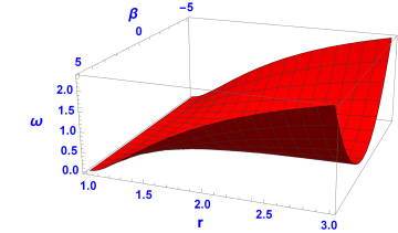
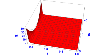
Figure 1: The behaviour of $\omega$ in the allowed region of the parameter space $(r,\beta)$ for both accelerating and decelerating phases for a particular case where $D=4$. Because of satisfaction of the weak energy condition, we have assumed $r>1/3$.

V Summary and Discussion

In Section §II, by employing a generalised procedure, we have established an extended version of the MSBT with an induced matter and a self-interacting scalar potential in arbitrary dimensional hypersurface. In particular, the SB field equations were derived from a generalised $(D+1)$-dimensional action. In this action, neither scalar potential nor cosmological constant have been considered. However, in order to extend the procedure used in the original IMT, we have assumed the bulk to contain ordinary matter.

Using a general and coordinate free framework, the geometrical quantities associated with the $(D+1)$-dimensional semi-Riemannian manifold have been related to those corresponding to a $D$-dimensional one. These general equations have been applied to the particular metric (16).

Using the latter relations for the SB field equations, we have established the $D$-dimensional SB field equations, in which the induced matter and the scalar potential have an intrinsic geometrical origin. One of the characteristic features of this model is that the reduction procedure generates the type of the induced potential.

We should emphasise that, due to the coordinate free framework we have used, our procedure to obtain the MSBT is much broader than those used to construct the standard IMT PW92 , MBDT RFM14 or MSBT RM18 .

As a cosmological application of the MSBT, we considered a universe that is described with an extended version of an FLRW metric in a $(D+1)$-dimensional space-time. By assuming a simple case in which there is no ordinary matter, we have shown that there are two constants of motion constructed from different functions of the three unknowns of the model. Then, we have obtained two distinct classes of exact solutions for the field equations. We have expressed the scale factors and the scalar field in terms of the cosmic time, such that for both of the classes, the scale factors do not explicitly depend on the parameter $n$ (see action (1)), whilst, the scalar field $\phi(t)$, depends on $n$, and it is given by two different functions of the cosmic time. Moreover, we have demonstrated how these solutions on the hypersurface correspond to the solutions obtained in the BD cosmology for the spatially flat FLRW universe; cf Section §III.

Subsequently, we have focused our attention to the cosmological solutions on the hypersurface. Accordingly, we have introduced useful physical quantities to analyze our solutions. Moreover, in order to clarify the reduced cosmology, we have also established the standard Friedmann equations (which are obtained for the spatially flat FLRW metric within the context of general relativity) on the hypersurface, whose (total) matter field in the right hand sides is composed of two non-interacting components: the induced matter (which directly emerges from the geometry of the extra dimension) and the matter associated with the SB scalar field $\phi$ (whose potential, according to our herein MSBT, has also geometrical origin).

As mentioned earlier, there are two distinct classes of solutions on the hypersurface. In what follows, in addition to presenting a summary of our two classes, we provide a complementary discussion.

Case I) Cosmological constant:

For the first class of solutions, we have found that a positive cosmological constant dominates, which is, surprisingly, obtained from superposition of two time dependent sectors. Consequently, the scale factor of the universe expands exponentially, which can be used to describe either inflation at the early universe or the acceleration at late times. However, the scalar field $\psi(t)$ decreases with comic time, which indicates that the extra dimension contracts or shrinks. Note that the so-called cosmological constant appearing in the effective field equations is not added by hand; it depends on the number of dimensions of the space time and the expansion rate of the scalar field $\psi(t)$ (i.e., the scale factor associated with the non-compact extra dimension).

In the solution associated with the spatially flat FLRW metric (43) within the context of IMT, the scale factor of the universe cannot ever accelerate. As the unique solution (48) indicates, in the context of the IMT, neither the cosmological constant nor an accelerating phase is obtained for the universe described with the FLRW metric (43). In order to convey a better understanding of the nature of the cosmological constant, the canonical metric has been employed in noncompact KK gravity, see, e.g., MLW94 ; MWL98 and related papers. For instance, on a $D$-dimensional hypersurface, we can find a correspondence between our asymptotic solution (i.e., the solution obtained in the particular case where $f(D)=0$) and that obtained in the IMT for the canonical metric

$$dS^{2}=\frac{y^{2}}{L^{2}}\tilde{g}_{\mu\nu}(x^{\alpha},y)dx^{\mu}dx^{\nu}-dy^{2},$$

where $L>0$ is a constant.

Let us consider a particular case where $T_{\mu\nu}^{{}^{(D+1)}}=0$, ${\tilde{g}}_{\mu\nu}={\rm diag}(1,-a^{2}(t),-a^{2}(t),...,-a^{2}(t))$ and $\phi=\phi(t)$. For this case, the induced matter (33) is given by

$$\chi T_{\mu\nu}^{{}^{(D)[{\rm eff}]}}=\frac{1}{2L^{2}}\left(D^{2}-3D+2+y_{0}^{2}V_{0}\right){\tilde{g}}_{\mu\nu},$$

where $y_{0}={\rm constant}$ is the value of $y$ on the hypersurface and the constant potential $V_{0}$ is obtained from (39). Therefore, Eq. (32) reduces to

$$G_{\mu\nu}^{{}^{(D)}}=\left(\frac{D^{2}-3D+2}{2L^{2}}\right){\tilde{g}}_{\mu\nu}+{\cal W}\phi^{n}\left[({\cal D}_{\mu}\phi)({\cal D}_{\nu}\phi)-\frac{y_{0}^{2}}{2L^{2}}({\cal D}_{\alpha}\phi)({\cal D}^{\alpha}\phi){\tilde{g}}_{\mu\nu}\right].$$

Then the SB cosmological solutions associated with the canonical gauge are given by

$$a(t) = a_{i}{\rm Exp}\left[\frac{(D-1)(t-t_{i})}{L}\right],$$

$$\phi(t) = \left\{\begin{array}[]{c}\Bigg{\{}\frac{CL(n+2)}{2(1-D)}{\rm Exp}\left[\frac{(1-D)(t-t_{i})}{L}\right]\Bigg{\}}^{\frac{2}{n+2}}\hskip 34.1433pt{\rm for}\hskip 22.76219ptn\neq-2,\\ \\ \Bigg{\{}{\rm Exp}\left[{\rm Exp}(\frac{(1-D)(t-t_{i})}{L})\right]\Bigg{\}}^{\frac{CL}{1-D}}\hskip 48.36967pt{\rm for}\hskip 22.76219ptn=-2,\end{array}\right.,$$ (128)

where $a_{i}$ and $t_{i}$ are integration constants and $C$ is the constant of motion given by $C\equiv a^{D-1}\phi^{\frac{n}{2}}\dot{\phi}$. Setting $\phi={\rm constant}$, we can easily show that our SB model reduces to the corresponding one obtained within the context of IMT, i.e., $G_{\mu\nu}=(D^{2}-3D+2){\tilde{g}}_{\mu\nu}/(2L^{2})$, in which $\Lambda=\Lambda(D)\equiv(D^{2}-3D+2)/(2L^{2})$; for the case where $D=4$, see, for instance, MWL98 ; P08 and references therein.

Case II) Power-law solutions:

The solutions of this case, in terms of the cosmic time, for both the $a(t)$, $\psi(t)$ and the induced scalar potential $V(t)$ are in power-law forms; while the SB scalar field $\phi(t)$ is in power-law and logarithmic forms for $n=-2$ and $n\neq-2$, respectively. We have shown that both the induced matter and the matter associated with the scalar field satisfy the barotropic EoS; they also obey the conservation law. Namely, the total matter in this case is composed of two non-interacting fluids. We have obtained the corresponding density parameters.

Subsequently, we have focused on the behaviour of the quantities for different values of the present parameters and integration constants. We have shown that it is feasible to get an accelerating universe. In this case, the total matter, the induced matter and the matter associated with $\phi$ could play the role of a dark energy. However, in the case of a decelerating universe, all three fluids play a role as ordinary matter in the universe for the allowed ranges of the parameters. We have discussed how to satisfy the weak energy condition for all kinds of matter. Furthermore, we have shown that for both the accelerating and the decelerating expansions, the large extra dimension contracts with cosmic time.

In what follows, let us further add some brief points.

• We have shown that the MSBT is described by four equations of motion (30), (32)(38) and (40). Concerning the cosmological example, which is described with the extended FLRW metric (43), in section IV, we just used Eqs. (32)-(38). As there is no ordinary matter in the bulk and the coefficient of the metric (43) as well as the scalar field depend on the cosmic time only (imposing the cylinder condition), therefore, (i) from Eq. (30), we obtain ${\cal D}^{2}\psi=0$, which is the Klein-Gordon equation for the massless scalar field. Moreover, $T^{{}^{(D)[{\rm eff}]}}=g^{\mu\nu}T_{\mu\nu}^{{}^{(D)[{\rm eff}]}}=V(\phi)/2\chi$, which indicates that, contrary to the IMT, the induced matter in the MSBT, even by imposing the cylinder condition and assuming a bulk in the absence of the ordinary matter, does necessarily consist of photons only. It is seen that Eq. (30), using the solutions (60), (61), (66), (67), is identically satisfied for all the values taken by $n$ and $f(D)$. (ii) Eq. (40) implies that $P_{\alpha\beta}$ is a conserved quantity.

• As in the particular cases where $n=-2$ and $n=0$, the SB framework transforms to the well-known canonical scalar field model (for $n=-2$, we can set $\phi\equiv Exp\left(\Phi\right)$), to demand non-ghost scalar fields, we should exclude the negative values of ${\cal W}$. However, for general cases where $n\neq-2,0$, determining whether or not the scalar field being a ghost field seems not only depend on the values of ${\cal W}$, but also the values of $n$ and the behavior of $\phi(t)$ at all times, which must be inspected carefully.

• To the best of our knowledge, the observational constraints on the parameters of the SB theory have not been studied. Such objectives were however beyond the scope of this work.

References

• (1) T. Kaluza, Sitz. Preuss. Akad. Wiss. 33, 966 (1921).
• (2) O. Klein, Z. Phys. 37, 895 (1926).
• (3) J.M. Overduin and P.S. Wesson, Phys. Rep. 283, 303 (1997).
• (4) P.S. Wesson and J. Ponce de Leon, J. Math. Phys. 33, 3883 (1992).
• (5) H. Liu and James M. Overduin, ApJ 538, 386 (2000).
• (6) James M. Overduin, Phys. Rev. D 62, 102001 (2000).
• (7) J. M. Overduin, P. S. Wesson, and B. Mashhoon, Astronomy and Astrophys. 473, 727 (2007).
• (8) N. Doroud, S.M. M. Rasouli and S. Jalalzadeh, Gen. Rel. Grav. 41, 2637 (2009).
• (9) J. Ponce de Leon, Class. Quant. Grav. 27, 095002 (2010).
• (10) S.M. M. Rasouli and S. Jalalzadeh, Ann. Phys. (Berlin) 19, 276 (2010).
• (11) S.M. M. Rasouli, M. Farhoudi and H.R. Sepangi, Class. Quant. Grav. 28, 155004 (2011).
• (12) S.M. M. Rasouli, M. Farhoudi and P. V. Moniz, Classical Quantum Gravity 31, 115002 (2014).
• (13) S. M. M. Rasouli and P. Moniz, Class. Quant. Grav. 33, 035006 (2016).
• (14) J. Socorro, Luis O. Pimentel, L. Toledo Sesma, Adv. High Energy Phys. 2018, 3658086 (2018).
• (15) S. M. M. Rasouli and P. Moniz, Class. Quant. Grav. 36, 075010 (2019).
• (16) P.S. Wesson, B. Mashhoon and J. M. Overduin, Int. J. Mod. Phys. D 17, 2527 (2008).
• (17) V. A. Rubakov and M. E. Shaposhnikov, Phys. Lett. 125B, 139 (1983).
• (18) A. Kehagias and K. Tamvakis, Mod. Phys. Lett. A 17, 1767 (2002).
• (19) Guang-Zhen Kang, De-Sheng Zhang, Hong-Shi Zong and Jun Li, “Fine Tuning Problem of the Cosmological Constant in a Generalized Randall-Sundrum Model”, arXive: 1906.05442.
• (20) P.S. Wesson, Phys. Lett. B 706, 1 (2011).
• (21) Valerio Faraoni, Int. J. Mod. Phys. D 11, 471 (2002).
• (22) Robert J. Nemiroff, Ravi Joshi and Bijunath R. Patla, JCAP 06, 006, (2015).
• (23) D. Sáez and V. J. Ballester,Phys. Lett.113A, 9, 1986.
• (24) M. Sabido, J. Socorro and L. Arturo Ureña-López, “Classical and quantum Cosmology of the Sáez-Ballester theory” Fizika B, 19, 177 (2010), arXiv:0904.0422.
• (25) S. Rippl, C. Romero and R. Tavakol, Class. Quant. Grav. 12, 2411 (1995).
• (26) S. M. M. Rasouli and P. V. Moniz, Class. Quantum Grav. 35 35, 025004 (2018).
• (27) B. O’Neil, “Semi-Riemannian Geometry (with applications to Relativity),” Academic Press, 1983.
• (28) N. Koiso, Ann. Sci. École Norm. Sup. (4) 14 (1981), no. 4, 433–443.
• (29) J. Ponce de Leon, J. Cosmol. Astropart. Phys. 03, 030 (2010).
• (30) Paul S. Wesson, James M. Overduin, “ The Scalar Field Source in Kaluza-Klein Theory”, arXiv:1307.4828.
• (31) V. Faraoni, Cosmology in Scalar Tensor Gravity (Kluiwer Academic Publishers, Netherlands, 2004).
• (32) Bahram Mashhoon, Hongya Liu and Paul Wesson, Phys. Lett. B 331, 305 (1994).
• (33) Bahram Mashhoon, Paul Wesson and Hongya Liu, Gen. Rel. Grav. 30, 4 (1998).
• (34) J. Ponce de Leon, Gravitation and Cosmology 14, 241 (2008).