A Bilingual Generative Transformer for Semantic Sentence Embedding

Abstract

Semantic sentence embedding models encode natural language sentences into vectors, such that closeness in embedding space indicates closeness in the semantics between the sentences. Bilingual data offers a useful signal for learning such embeddings: properties shared by both sentences in a translation pair are likely semantic, while divergent properties are likely stylistic or language-specific. We propose a deep latent variable model that attempts to perform source separation on parallel sentences, isolating what they have in common in a latent semantic vector, and explaining what is left over with language-specific latent vectors. Our proposed approach differs from past work on semantic sentence encoding in two ways. First, by using a variational probabilistic framework, we introduce priors that encourage source separation, and can use our model’s posterior to predict sentence embeddings for monolingual data at test time. Second, we use high-capacity transformers as both data generating distributions and inference networks – contrasting with most past work on sentence embeddings. In experiments, our approach substantially outperforms the state-of-the-art on a standard suite of unsupervised semantic similarity evaluations. Further, we demonstrate that our approach yields the largest gains on more difficult subsets of these evaluations where simple word overlap is not a good indicator of similarity.

1 Introduction

Learning useful representations of language has been a source of recent success in natural language processing (NLP). Much work has been done on learning representations for words (Mikolov et al., 2013; Pennington et al., 2014) and sentences (Kiros et al., 2015; Conneau et al., 2017). More recently, deep neural architectures have been used to learn contextualized word embeddings (Peters et al., 2018; Devlin et al., 2018) enabling state-of-the-art results on many tasks. We focus on learning semantic sentence embeddings in this paper, which play an important role in many downstream applications. Since they do not require any labelled data for fine-tuning, sentence embeddings are useful out-of-the-box for problems such as measurement of Semantic Textual Similarity (STS; Agirre et al. (2012)), mining bitext (Zweigenbaum et al., 2018), and paraphrase identification (Dolan et al., 2004). Semantic similarity measures also have downstream uses such as fine-tuning machine translation systems (Wieting et al., 2019a).

There are three main ingredients when designing a sentence embedding model: the architecture, the training data, and the objective function. Many architectures including LSTMs (Hill et al., 2016; Conneau et al., 2017; Schwenk and Douze, 2017; Subramanian et al., 2018), Transformers (Cer et al., 2018; Reimers and Gurevych, 2019), and averaging models (Wieting et al., 2016b; Arora et al., 2017) are capable of learning sentence embeddings. The choice of training data and objective are intimately intertwined, and there are a wide variety of options including next-sentence prediction (Kiros et al., 2015), machine translation (Espana-Bonet et al., 2017; Schwenk and Douze, 2017; Schwenk, 2018; Artetxe and Schwenk, 2018), natural language inference (NLI)  (Conneau et al., 2017), and multi-task objectives which include some of the previously mentioned objectives (Cer et al., 2018) potentially combined with additional tasks like constituency parsing (Subramanian et al., 2018).

Surprisingly, despite ample testing of more powerful architectures, the best performing models for many sentence embedding tasks related to semantic similarity often use simple architectures that are mostly agnostic to the interactions between words. For instance, some of the top performing techniques use word embedding averaging (Wieting et al., 2016b), character n-grams (Wieting et al., 2016a), and subword embedding averaging (Wieting et al., 2019b) to create representations. These simple approaches are competitive with much more complicated architectures on in-domain data and generalize well to unseen domains, but are fundamentally limited by their inability to capture word order. Training these approaches generally relies on discriminative objectives defined on paraphrase data (Ganitkevitch et al., 2013; Wieting and Gimpel, 2018) or bilingual data (Wieting et al., 2019b; Chidambaram et al., 2019; Yang et al., 2020). The inclusion of latent variables in these models has also been explored (Chen et al., 2019).

Intuitively, bilingual data in particular is promising because it potentially offers a useful signal for learning the underlying semantics of sentences. Within a translation pair, properties shared by both sentences are more likely semantic, while those that are divergent are more likely stylistic or language-specific. While previous work learning from bilingual data perhaps takes advantage of this fact implicitly, the focus of this paper is modelling this intuition explicitly, and to the best of our knowledge, this has not been explored in prior work. Specifically, we propose a deep generative model that is encouraged to perform source separation on parallel sentences, isolating what they have in common in a latent semantic embedding and explaining what is left over with language-specific latent vectors. At test time, we use inference networks (Kingma and Welling, 2013) for approximating the model’s posterior on the semantic and source-separated latent variables to encode monolingual sentences. Finally, since our model and training objective are generative, our approach does not require knowledge of the distance metrics to be used during evaluation, and it has the additional property of being able to generate text.

In experiments, we evaluate our probabilistic source-separation approach on a standard suite of STS evaluations. We demonstrate that the proposed approach is effective, most notably allowing the learning of high-capacity deep Transformer architectures (Vaswani et al., 2017) while still generalizing to new domains, significantly outperforming a variety of state-of-the-art baselines. Further, we conduct a thorough analysis by identifying subsets of the STS evaluation where simple word overlap is not able to accurately assess semantic similarity. On these most difficult instances, we find that our approach yields the largest gains, indicating that our system is modeling interactions between words to good effect. We also find that our model better handles cross-lingual semantic similarity than multilingual translation baseline approaches, indicating that stripping away language-specific information allows for better comparisons between sentences from different languages.

Finally, we analyze our model to uncover what information was captured by the source separation into the semantic and language-specific variables and the relationship between this encoded information and language distance to English. We find that the language-specific variables tend to explain more superficial or language-specific properties such as overall sentence length, amount and location of punctuation, and the gender of articles (if gender is present in the language), but semantic and syntactic information is more concentrated in the shared semantic variables, matching our intuition. Language distance has an effect as well, where languages that share common structures with English put more information into the semantic variables, while more distant languages put more information into the language-specific variables. Lastly, we show outputs generated from our model that exhibit its ability to do a type of style transfer.

2 Model

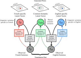
Figure 1: The generative process of our model. Latent variables modeling the linguistic variation in French and English, $z_{fr}$ and $z_{en}$, as well as a latent variable modeling the common semantics, $z_{sem}$, are drawn from a multivariate Gaussian prior. The observed text in each language is then conditioned on its language-specific variable and $z_{sem}$.

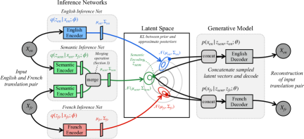
Figure 2: The computation graph for the variational lower bound used during training. The English and French text are fed into their respective inference networks and the semantic inference network to ultimately produce the language variables $z_{fr}$ and $z_{en}$ and semantic variable $z_{sem}$. Each language-specific variable is then concatenated to $z_{sem}$ and used by the decoder to reconstruct the input sentence pair.

Our proposed training objective leverages a generative model of parallel text in two languages. Our model is language agnostic, and applies to a wide variety of languages (see Section 5) but we will use the running example of English (en) and French (fr) pairs consisting of an English sentence $x_{en}$ and a French sentence $x_{fr}$. Importantly, the generative process utilizes three underlying latent vectors: language-specific variation variables (language variables) $z_{fr}$ and $z_{en}$ for each side of the translation, as well as a shared semantic variation variable (semantic variable) $z_{sem}$. In this section we will first describe the generative model for the text and latent variables. In the following section we will describe the inference procedure of $z_{sem}$ given an input sentence, which corresponds to our core task of obtaining sentence embeddings useful for downstream tasks such as semantic similarity.

The generative process of our model, the Bilingual Generative Transformer (BGT), is depicted in Figure 1 and the training computation graph is shown in Figure 2. First, we sample latent variables $\langle z_{fr},z_{en},z_{sem}\rangle$, where $z_{i}\in\mathbb{R}^{k}$, from a multivariate Gaussian prior $\mathcal{N}(0,I_{k})$. These variables are then fed into a decoder that samples sentences; $x_{en}$ is sampled conditioned on $z_{sem}$ and $z_{en}$, while $x_{fr}$ is sampled conditioned on $z_{sem}$ and $z_{fr}$. Because sentences in both languages will use $z_{sem}$ in generation, we expect that in a well-trained model this variable will encode semantic, syntactic, or stylistic information shared across both sentences, while $z_{fr}$ and $z_{en}$ will handle any language-specific peculiarities or specific stylistic decisions that are less central to the sentence meaning and thus do not translate across sentences. In the following section, we further discuss how this is explicitly encouraged by the learning process.

Decoder Architecture. Many latent variable models for text use LSTMs (Hochreiter and Schmidhuber, 1997) as their decoders (Yang et al., 2017; Ziegler and Rush, 2019; Ma et al., 2019). However, state-of-the-art models in neural machine translation have seen increased performance and speed using deep Transformer architectures. We also found in our experiments (see Appendix C for details) that Transformers led to increased performance in our setting, so they are used in our main model.

We use two decoders in our model, one for modelling $p(x_{fr}|z_{sem},z_{fr};\theta)$ and one for modeling $p(x_{en}|z_{sem},z_{en};\theta)$ (see right side of Figure 2). Each decoder takes in a language variable and a semantic variable, which are concatenated and used by the decoder for reconstruction. We explore four ways of using this latent vector: (1) Concatenate it to the word embeddings (Word) (2) Use it as the initial hidden state (Hidden, LSTM only) (3) Use it as you would the attention context vector in the traditional sequence-to-sequence framework (Attention) and (4) Concatenate it to the hidden state immediately prior to computing the logits (Logit). Unlike Attention, there is no additional feedforward layer in this setting. We experimented with these four approaches, as well as combinations thereof, and report this analysis in Appendix A. From these experiments, we see that the closer the sentence embedding is to the final word predictor, the better the performance on downstream tasks evaluating its semantic content. We hypothesise that this is due to better gradient propagation because the sentence embedding is now closer to the error signal. Since Attention and Logit performed best, we use these in our main experiments.

3 Learning and Inference

Our model is trained on a set of parallel sentences $X$ consisting of $N$ examples, $X=\{\langle x^{1}_{en},x^{1}_{fr}\rangle,\ldots,\langle x^{N}_{en},x^{N}_{fr}\rangle\}$, and $Z$ is our collection of latent variables $Z=(\langle z^{1}_{en},z^{1}_{fr},z^{1}_{sem}\rangle,\ldots,\langle z^{N}_{en},z^{N}_{fr},z^{N}_{sem}\rangle)$. We wish to maximize the likelihood of the parameters of the two decoders $\theta$ with respect to the observed $X$, marginalizing over the latent variables $Z$.

$$p(X;\theta)=\int_{Z}p(X,Z;\theta)dZ$$

Unfortunately, this integral is intractable due to the complex relationship between $X$ and $Z$. However, related latent variable models like variational autoencoders (VAEs; Kingma and Welling (2013)) learn by optimizing a variational lower bound on the log marginal likelihood. This surrogate objective is called the evidence lower bound (ELBO) and introduces a variational approximation, $q$ to the true posterior of the model $p$. The $q$ distribution is parameterized by a neural network with parameters $\phi$. ELBO for our model is written as:

$$\text{ELBO}= \mathbb{E}_{q(Z|X;\phi)}[\log p(X|Z;\theta)]-$$

$$\text{KL}(q(Z|X;\phi)||p(Z;\theta))$$

This lower bound on the marginal can be optimized by gradient ascent by using the reparameterization trick (Kingma and Welling, 2013). This trick allows for the expectation under $q$ to be approximated through sampling in a way that preserves backpropagation. We make several independence assumptions for $q(z_{sem},z_{en},z_{fr}|x_{en},x_{fr};\phi)$ to match our goal of source separation: we factor $q$ as $q(z_{sem}|x_{en},x_{fr};\phi)q(z_{en}|x_{en};\phi)q(z_{fr}|x_{fr};\phi)$. The parameters of the encoders that make up the inference networks, defined in the next paragraph, are denoted as $\phi$.

Lastly, we note that the KL term in our ELBO equation explicitly encourages explaining variation that is shared by translations with the shared semantic variable, and explaining language-specific variation with the corresponding language-specific variables. Encoding information shared by the two sentences in the shared variable results in only a single penalty from the KL loss, while encoding the information separately in both language specific variables will cause unnecessary replication, doubling the overall cost incurred by the KL term.

Encoder Architecture.

We use three inference networks as shown on the left side of Figure 2: an English inference network to produce the English language variable, a French inference network to produce the French language variable, and a semantic inference network to produce the semantic variable. Just as in the decoder architecture, we use a Transformer for the encoders.

The semantic inference network is a bilingual encoder that encodes each language. For each translation pair, we alternate which of the two parallel sentences is fed into the semantic encoder within a batch. Since the semantic encoder is meant to capture language agnostic semantic information, its outputs for a translation pair should be similar regardless of the language of the input sentence. We note that other operations are possible for combining the views each parallel sentence offers. For instance, we could feed both sentences into the semantic encoder and pool their representations. However, in practice we find that alternating works well and also can be used to obtain sentence embeddings for text that is not part of a translation pair. We leave further study of combining views to future work.

4 Experiments

4.1 Baseline Models

We experiment with fourteen baseline models, covering both the most effective approaches for learning sentence embeddings from the literature and ablations of our own BGT model. These baselines can be split into three groups as detailed below.

Models from the Literature (Trained on Different Data)

We compare to well known sentence embedding models Infersent (Conneau et al., 2017), GenSen (Subramanian et al., 2018), the Universal Sentence Encoder (USE) (Cer et al., 2018), LASER Artetxe and Schwenk (2018), as well as BERT (Devlin et al., 2018). We used the pretrained BERT model in two ways to create a sentence embedding. The first way is to concatenate the hidden states for the CLS token in the last four layers. The second way is to concatenate the hidden states of all word tokens in the last four layers and mean pool these representations. Both methods result in a 4096 dimension embedding. We also compare to the newly released model, Sentence-Bert (Reimers and Gurevych, 2019). This model is similar to Infersent (Conneau et al., 2017) in that it is trained on natural language inference data, SNLI (Bowman et al., 2015). However, instead of using pretrained word embeddings, they fine-tune BERT in a way to induce sentence embeddings.

Models from the Literature (Trained on Our Data)

These models are amenable to being trained in the exact same setting as our own models as they only require parallel text. These include the sentence piece averaging model, SP, from Wieting et al. (2019b), which is among the best of the averaging models (i.e. compared to averaging only words or character $n$-grams) as well the LSTM model, BiLSTM, from Wieting and Gimpel (2017). These models use a contrastive loss with a margin. Following their settings, we fix the margin to 0.4 and tune the number of batches to pool for selecting negative examples from $\{40,60,80,100\}$. For both models, we set the dimension of the embeddings to 1024. For BiLSTM, we train a single layer bidirectional LSTM with hidden states of 512 dimensions. To create the sentence embedding, the forward and backward hidden states are concatenated and mean-pooled. Following Wieting and Gimpel (2017), we shuffle the inputs with probability $p$, tuning $p$ from $\{0.3,0.5\}$.

We also implicitly compare to previous machine translation approaches like Espana-Bonet et al. (2017); Schwenk and Douze (2017); Artetxe and Schwenk (2018) in Appendix A where we explore different variations of training LSTM sequence-to-sequence models. We find that our translation baselines reported in the tables below (both LSTM and Transformer) outperform the architectures from these works due to using the Attention and Logit methods mentioned in Section 2, demonstrating that our baselines represent, or even over-represent, the state-of-the-art for machine translation approaches.

BGT Ablations

Lastly, we compare to ablations of our model to better understand the benefits of parallel data, language-specific variables, the KL loss term, and how much we gain from the more conventional translation baselines.

• EnglishAE: English autoencoder on the English side of our en-fr data.

• EnglishVAE: English variational autoencoder on the English side of our en-fr data.

• EnglishTrans: Translation from en to fr.

• BilingualTrans: Translation from both en to fr and fr to en where the encoding parameters are shared but each language has its own decoder.

• BGT w/o LangVars: A model similar to BilingualTrans, but it includes a prior over the embedding space and therefore a KL loss term. This model differs from BGT since it does not have any language-specific variables.

• BGT w/o Prior: Follows the same architecture as BGT, but without the priors and KL loss term.

4.2 Experimental Settings

Data	Sentence 1	Sentence 2	Gold Score
Hard+	Other ways are needed.	It is necessary to find other means.	4.5
Hard-	How long can you keep chocolate in the freezer?	How long can I keep bread dough in the refrigerator?	1.0
Negation	It’s not a good idea.	It’s a good idea to do both.	1.0

Table 1: Examples from our Hard STS dataset and our negation split. The sentence pair in the first row has dissimilar structure and vocabulary yet a high gold score. The second sentence pair has similar structure and vocabulary and a low gold score. The last sentence pair contains negation, where there is a not in Sentence 1 that causes otherwise similar sentences to have low semantic similarity.

The training data for our models is a mixture of OpenSubtitles 2018 en-fr data and en-fr Gigaword data. To create our dataset, we combined the complete corpora of each dataset and then randomly selected 1,000,000 sentence pairs to be used for training with 10,000 used for validation. We use sentencepiece (Kudo and Richardson, 2018) with a vocabulary size of 20,000 to segment the sentences, and we chose sentence pairs whose sentences are between 5 and 100 tokens each.

In designing the model architectures for the encoders and decoders, we experimented with Transformers and LSTMs. Due to better performance, we use a 5 layer Transformer for each of the encoders and a single layer decoder for each of the decoders. This design decision was empirically motivated as we found using a larger decoder was slower and worsened performance, but conversely, adding more encoder layers improved performance. More discussion of these trade-offs along with ablations and comparisons to LSTMs are included in Appendix C.

For all of our models, we set the dimension of the embeddings and hidden states for the encoders and decoders to 1024. Since we experiment with two different architectures, we follow two different optimization strategies. For training models with Transformers, we use Adam (Kingma and Ba, 2014) with $\beta_{1}=0.9$, $\beta_{2}=0.98$, and $\epsilon=10^{-8}$. We use the same learning rate schedule as Vaswani et al. (2017), i.e., the learning rate increases linearly for 4,000 steps to $5\times 10^{-4}$, after which it is decayed proportionally to the inverse square root of the number of steps. For training the LSTM models, we use Adam with a fixed learning rate of 0.001. We train our models for 20 epochs.

For models incorporating a translation loss, we used label smoothed cross entropy (Szegedy et al., 2016; Pereyra et al., 2017) with $\epsilon=0.1$. For EnglishVAE, BGT and BilingualTrans, we anneal the KL term so that it increased linearly for $2^{16}$ updates, which robustly gave good results in preliminary experiments. We also found that in training BGT, combining its loss with the BilingualTrans objective during training of both models increased performance, and so this loss was summed with the BGT loss in all of our experiments. We note that this does not affect our claim of BGT being a generative model, as this loss is only used in a multi-task objective at training time, and we calculate the generation probabilities according to standard BGT at test time.

Lastly, in Appendix B, we illustrate that it is crucial to train the Transformers with large batch sizes. Without this, the model can learn the goal task (such as translation) with reasonable accuracy, but the learned semantic embeddings are of poor quality until batch sizes approximately reach 25,000 tokens. Therefore, we use a maximum batch size of 50,000 tokens in our EnglishTrans, BilingualTrans, and BGT w/o Prior, experiments and 25,000 tokens in our BGT w/o LangVars and BGT experiments.

Model	Semantic Textual Similarity (STS)
	2012	2013	2014	2015	2016	Avg.	Hard+	Hard-	Avg.
BERT (CLS)	33.2	29.6	34.3	45.1	48.4	38.1	7.8	12.5	10.2
BERT (Mean)	48.8	46.5	54.0	59.2	63.4	54.4	3.1	24.1	13.6
Infersent	61.1	51.4	68.1	70.9	70.7	64.4	4.2	29.6	16.9
GenSen	60.7	50.8	64.1	73.3	66.0	63.0	24.2	6.3	15.3
USE	61.4	59.0	70.6	74.3	73.9	67.8	16.4	28.1	22.3
LASER	63.1	47.0	67.7	74.9	71.9	64.9	18.1	23.8	20.9
Sentence-BERT	66.9	63.2	74.2	77.3	72.8	70.9	23.9	3.6	13.8
SP	68.4	60.3	75.1	78.7	76.8	71.9	19.1	29.8	24.5
BiLSTM	67.9	56.4	74.5	78.2	75.9	70.6	18.5	23.2	20.9
EnglishAE	60.2	52.7	68.6	74.0	73.2	65.7	15.7	36.0	25.9
EnglishVAE	59.5	54.0	67.3	74.6	74.1	65.9	16.8	42.7	29.8
EnglishTrans	66.5	60.7	72.9	78.1	78.3	71.3	18.0	47.2	32.6
BilingualTrans	67.1	61.0	73.3	78.0	77.8	71.4	20.0	48.2	34.1
BGT w/o LangVars	68.3	61.3	74.5	79.0	78.5	72.3	24.1	46.8	35.5
BGT w/o Prior	67.6	59.8	74.1	78.4	77.9	71.6	17.9	45.5	31.7
BGT	68.9	62.2	75.9	79.4	79.3	73.1	22.5	46.6	34.6

Table 2: Results of our models and models from prior work. The first six rows are pretrained models from the literature, the next two rows are strong baselines trained on the same data as our models, and the last seven rows include model ablations and BGT, our final model. We show results, measured in Pearson’s $r\times 100$, for each year of the STS tasks 2012-2016 and our two Hard STS datasets.

Model	es-es	ar-ar	en-es	en-ar	en-tr
LASER	79.7	69.3	59.7	65.5	72.0
BilingualTrans	83.4	72.6	64.1	37.6	59.1
BGT w/o LangVars	81.7	72.8	72.6	73.4	74.8
BGT w/o Prior	84.5	73.2	68.0	66.5	70.9
BGT	85.7	74.9	75.6	73.5	74.9

Table 3: Performance measured in Pearson’s $r\times 100$, on the SemEval 2017 STS task on the es-es, ar-ar, en-es, en-ar, and en-tr datasets.

4.3 Evaluation

Our primary evaluation are the 2012-2016 SemEval Semantic Textual Similarity (STS) shared tasks (Agirre et al., 2012, 2013, 2014, 2015, 2016), where the goal is to accurately predict the degree to which two sentences have the same meaning as measured by human judges. The evaluation metric is Pearson’s $r$ with the gold labels.

Secondly, we evaluate on Hard STS, where we combine and filter the STS datasets in order to make a more difficult evaluation. We hypothesize that these datasets contain many examples where their gold scores are easy to predict by either having similar structure and word choice and a high score or dissimilar structure and word choice and a low score. Therefore, we split the data using symmetric word error rate (SWER), finding sentence pairs with low SWER and low gold scores as well as sentence pairs with high SWER and high gold scores. This results in two datasets, Hard+ which have SWERs in the bottom 20% of all STS pairs and whose gold label is between 0 and 1, and Hard- where the SWERs are in the top 20% of the gold scores are between 4 and 5. We also evaluate on a split where negation was likely present in the example. Examples are shown in Table 1.

Lastly, we evaluate on STS in es and ar as well as cross-lingual evaluations for en-es, en-ar, and en-tr. We use the datasets from SemEval 2017 (Cer et al., 2017). For this setting, we train BilingualTrans and BGT on 1 million examples from en-es, en-ar, and en-tr OpenSubtitles 2018 data.

4.4 Results

Model	Semantic Textual Similarity (STS)
	2012	2013	2014	2015	2016	Hard+	Hard-
Random Encoder	51.4	34.6	52.7	52.3	49.7	4.8	17.9
English Language Encoder	44.4	41.7	53.8	62.4	61.7	15.3	26.5
Semantic Encoder	68.9	62.2	75.9	79.4	79.3	22.5	46.6

Table 4: STS performance on the 2012-2016 datasets and our STS Hard datasets for a randomly initialized Transformer, the trained English language-specific encoder from BGT, and the trained semantic encoder from BGT. Performance is measured in Pearson’s $r\times 100$.

Lang.	Model	STS	S. Num.	O. Num.	Depth	Top Con.	Word	Len.	P. Num.	P. First	Gend.
fr	BilingualTrans	71.2	78.0	76.5	28.2	65.9	80.2	74.0	56.9	88.3	53.0
	Semantic Encoder	72.4	84.6	80.9	29.7	70.5	77.4	73.0	60.7	87.9	52.6
	en Language Encoder	56.8	75.2	72.0	28.0	63.6	65.4	80.2	65.3	92.2	-
	fr Language Encoder	-	-	-	-	-	-	-	-	-	56.5
es	BilingualTrans	70.5	84.5	82.1	29.7	68.5	79.2	77.7	63.4	90.1	54.3
	Semantic Encoder	72.1	85.7	83.6	32.5	71.0	77.3	76.7	63.1	89.9	52.6
	en Language Encoder	55.8	75.7	73.7	29.1	63.9	63.3	80.2	64.2	92.7	-
	es Language Encoder	-	-	-	-	-	-	-	-	-	54.7
ar	BilingualTrans	70.2	77.6	74.5	28.1	67.0	77.5	72.3	57.5	89.0	-
	Semantic Encoder	70.8	81.9	80.8	32.1	71.7	71.9	73.3	61.8	88.5	-
	en Language Encoder	58.9	76.2	73.1	28.4	60.7	71.2	79.8	63.4	92.4	-
tr	BilingualTrans	70.7	78.5	74.9	28.1	60.2	78.4	72.1	54.8	87.3	-
	Semantic Encoder	72.3	81.7	80.2	30.6	66.0	75.2	72.4	59.3	86.7	-
	en Language Encoder	57.8	77.3	74.4	28.3	63.1	67.1	79.7	67.0	92.5	-
ja	BilingualTrans	71.0	66.4	64.6	25.4	54.1	76.0	67.6	53.8	87.8	-
	Semantic Encoder	71.9	68.0	66.8	27.5	58.9	70.1	68.7	52.9	86.6	-
	en Language Encoder	60.6	77.6	76.4	28.0	64.6	70.0	80.4	62.8	92.0	-

Table 5: Average STS performance for the 2012-2016 datasets, measured in Pearson’s $r\times 100$, followed by probing results on predicting number of subjects, number of objects, constituent tree depth, top constituent, word content, length, number of punctuation marks, the first punctuation mark, and whether the articles in the sentence are the correct gender. All probing results are measured in accuracy $\times 100$.

The results on the STS and Hard STS are shown in Table 2. From the results, we see that BGT has the highest overall performance. It does especially well compared to prior work on the two Hard STS datasets. We used paired bootstrap resampling to check whether BGT significantly outperforms SentenceBert, SP, BilingualTrans, and BGT w/o Prior on the STS task. We found all gains to be significant with $p<0.01$.

From these results, we see that both positive examples that have little shared vocabulary and structure and negative examples with significant shared vocabulary and structure benefit significantly from using a deeper architecture. Similarly, examples where negation occurs also benefit from our deeper model. These examples are difficult because more than just the identity of the words is needed to determine the relationship of the two sentences, and this is something that SP is not equipped for since it is unable to model word order. The bottom two rows show easier examples where positive examples have high overlap and low SWER and vice versa for negative examples. Both models perform similarly on this data, with the BGT model having a small edge consistent with the overall gap between these two models.

Lastly, in Table 3, we show the results of STS evaluations in es and ar and cross-lingual evaluations for en-es, en-ar, and en-tr. We also include a comparison to LASER, which is a multilingual model. From these results, we see that BGT has the best performance across all datasets, however the performance is significantly stronger than the BilingualTrans and BGT w/o Prior baselines in the cross-lingual setting. Since BGT w/o LangVars also has significantly better performance on these tasks, most of this gain seems to be due to the prior having a regularizing effect. However, BGT outperforms BGT w/o LangVars overall, and we hypothesize that the gap in performance between these two models is due to BGT being able to strip away the language-specific information in the representations with its language-specific variables, allowing for the semantics of the sentences to be more directly compared.

5 Analysis

We next analyze our BGT model by examining what elements of syntax and semantics the language and semantic variables capture relative both to each-other and to the sentence embeddings from the BilingualTrans models. We also analyze how the choice of language and its lexical and syntactic distance from English affects the semantic and syntactic information captured by the semantic and language-specific encoders. Finally, we also show that our model is capable of sentence generation in a type of style transfer, demonstrating its capabilities as a generative model.

5.1 STS

We first show that the language variables are capturing little semantic information by evaluating the learned English language-specific variable from our BGT model on our suite of semantic tasks. The results in Table 4 show that these encoders perform closer to a random encoder than the semantic encoder from BGT. This is consistent with what we would expect to see if they are capturing extraneous language-specific information.

5.2 Probing

We probe our BGT semantic and language-specific encoders, along with our BilingualTrans encoders as a baseline, to compare and contrast what aspects of syntax and semantics they are learning relative to each other across five languages with various degrees of similarity with English. All models are trained on the OpenSubtitles 2018 corpus. We use the datasets from Conneau et al. (2018) for semantic tasks like number of subjects and number of objects, and syntactic tasks like tree depth, and top constituent. Additionally, we include predicting the word content and sentence length. We also add our own tasks to validate our intuitions about punctuation and language-specific information. In the first of these, punctuation number, we train a classifier to predict the number of punctuation marks in a sentence. To make the task more challenging, we limit each label to have at most 20,000 examples split among training, validation, and testing data. In the second task, punctuation first, we train a classifier to predict the identity of the first punctuation mark in the sentence. In our last task, gender, we detect examples where the gender of the articles in the sentence is incorrect in French or Spanish. To create an incorrect example, we switch articles from $\{$le, la, un, une$\}$ for French and $\{$el, la, los, las$\}$ for Spanish, with their (indefinite or definite for French and singular or plural for Spanish) counterpart with the opposite gender. This dataset was balanced so random chance gives 50% on the testing data. All tasks use 100,000 examples for training and 10,000 examples for validation and testing. The results of these experiments are shown in Table 5.

These results show that the source separation is effective - stylistic and language-specific information like length, punctuation and language-specific gender information are more concentrated in the language variables, while word content, semantic and syntactic information are more concentrated in the semantic encoder. The choice of language is also seen to be influential on what these encoders are capturing. When the languages are closely related to English, like in French and Spanish, the performance difference between the semantic and English language encoder is larger for word content, subject number, object number than for more distantly related languages like Arabic and Turkish. In fact, word content performance is directly tied to how well the alphabets of the two languages overlap. This relationship matches our intuition, because lexical information will be cheaper to encode in the semantic variable when it is shared between the languages. Similarly for the tasks of length, punctuation first, and punctuation number, the gap in performance between the two encoders also grows as the languages become more distant from English. Lastly, the gap on STS performance between the two encoders shrinks as the languages become more distant, which again is what we would expect, as the language-specific encoders are forced to capture more information.

Japanese is an interesting case in these experiments, where the English language-specific encoder outperforms the semantic encoder on the semantic and syntactic probing tasks. Japanese is a very distant language to English both in its writing system and in its sentence structure (it is an SOV language, where English is an SVO language). However, despite these difference, the semantic encoder strongly outperforms the English language-specific encoder, suggesting that the underlying meaning of the sentence is much better captured by the semantic encoder.

5.3 Generation and Style Transfer

Source	you know what i’ve seen?
Style	he said, “since when is going fishing” had anything to do with fish?”
Output	he said, “what is going to do with me since i saw you?”
Source	guys, that was the tech unit.
Style	is well, “capicci” …
Output	is that what, “technician”?
Source	the pay is no good, but it’s money.
Style	do we know cause of death?
Output	do we have any money?
Source	we’re always doing stupid things.
Style	all right listen, i like being exactly where i am,
Output	all right, i like being stupid, but i am always here.

Table 6: Style transfer generations from our learned BGT model. Source refers to the sentence fed into the semantic encoder, Style refers to the sentence fed into the English language-specific encoder, and Output refers to the text generated by our model.

In this section, we qualitatively demonstrate the ability of our model to generate sentences. We focus on a style-transfer task where we have original seed sentences from which we calculate our semantic vector $z_{sem}$ and language specific vector $z_{en}$. Specifically, we feed in a Source sentence into the semantic encoder to obtain $z_{sem}$, and another Style sentence into the English language-specific encoder to obtain $z_{en}$. We then generate a new sentence using these two latent variables. This can be seen as a type of style transfer where we expect the model to generate a sentence that has the semantics of the Source sentence and the style of the Style sentence. We use our en-fr BGT model from Table 5 and show some examples in Table 6. All input sentences are from held-out en-fr OpenSubtitles data. From these examples, we see further evidence of the role of the semantic and language-specific encoders, where most of the semantics (e.g. topical word such as seen and tech in the Source sentence) are reflected in the output, but length and structure are more strongly influenced by the language-specific encoder.

6 Conclusion

We propose Bilingual Generative Transformers, a model that uses parallel data to learn to perform source separation of common semantic information between two languages from language-specific information. We show that the model is able to accomplish this source separation through probing tasks and text generation in a style-transfer setting. We find that our model bests all baselines on unsupervised semantic similarity tasks, with the largest gains coming from a new challenge we propose as Hard STS, designed to foil methods approximating semantic similarity as word overlap. We also find our model to be especially effective on unsupervised cross-lingual semantic similarity, due to its stripping away of language-specific information allowing for the underlying semantics to be more directly compared. In future work, we will explore generalizing this approach to the multilingual setting, or applying it to the pre-train and fine-tune paradigm used widely in other models such as BERT.

-

Appendix A Location of Sentence Embedding in Decoder for Learning Representations

As mentioned in Section 2, we experimented with 4 ways to incorporate the sentence embedding into the decoder: Word, Hidden, Attention, and Logit. We also experimented with combinations of these 4 approaches. We evaluate these embeddings on the STS tasks and show the results, along with the time to train the models 1 epoch in Table 7.

For these experiments, we train a single layer bidirectional LSTM (BiLSTM) EnglishTrans model with embedding size set to 1024 and hidden states set to 512 dimensions (in order to be roughly equivalent to our Transformer models). To form the sentence embedding in this variant, we mean pool the hidden states for each time step. The cell states of the decoder are initialized to the zero vector.

Architecture	STS	Time (s)
BiLSTM (Hidden)	54.3	1226
BiLSTM (Word)	67.2	1341
BiLSTM (Attention)	68.8	1481
BiLSTM (Logit)	69.4	1603
BiLSTM (Wd. + Hd.)	67.3	1377
BiLSTM (Wd. + Hd. + Att.)	68.3	1669
BiLSTM (Wd. + Hd. + Log.)	69.1	1655
BiLSTM (Wd. + Hd. + Att. + Log.)	68.9	1856

Table 7: Results for different ways of incorporating the sentence embedding in the decoder for a BiLSTM on the Semantic Textual Similarity (STS) datasets, along with the time taken to train the model for 1 epoch. Performance is measured in Pearson’s $r\times 100$.

From this analysis, we see that the best performance is achieved with Logit, when the sentence embedding is place just prior to the softmax. The performance is much better than Hidden or Hidden+Word used in prior work. For instance, recently (Artetxe and Schwenk, 2018) used the Hidden+Word strategy in learning multilingual sentence embeddings.

A.1 VAE Training

We also found that incorporating the latent code of a VAE into the decoder using the Logit strategy increases the mutual information while having little effect on the log likelihood. We trained two LSTM VAE models following the settings and aggressive training strategy in (He et al., 2019), where one LSTM model used the Hidden strategy and the other used the Hidden + Logit strategy. We trained the models on the en side of our en-fr data. We found that the mutual information increased form 0.89 to 2.46, while the approximate negative log likelihood, estimated by importance weighting, increased slightly from 53.3 to 54.0 when using Logit.

Appendix B Relationship Between Batch Size and Performance for Transformer and LSTM

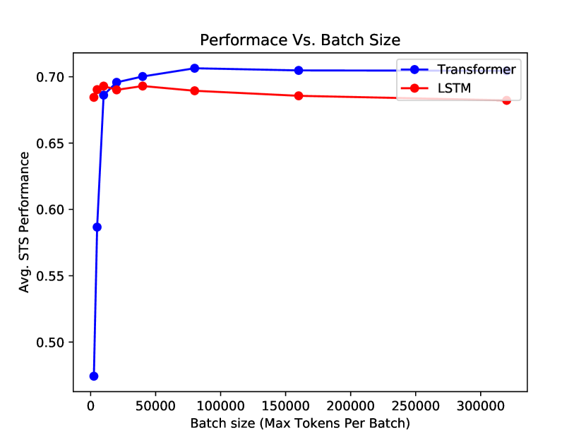
Figure 3: The relationship between average performance for each year of the STS tasks 2012-2016 (Pearson’s $r\times 100$) and batch size (maximum number of words per batch).

Data Split	$n$	BGT	SP
All	13,023	75.3	74.1
Negation	705	73.1	68.7
Bottom 20% SWER, label $\in[0,2]$	404	63.6	54.9
Bottom 10% SWER, label $\in[0,1]$	72	47.1	22.5
Top 20% SWER, label $\in[3,5]$	937	20.0	14.4
Top 10% SWER, label $\in[4,5]$	159	18.1	10.8
Top 20% SWER, label $\in[0,2]$	1380	51.5	49.9
Bottom 20% SWER, label $\in[3,5]$	2079	43.0	42.2

Table 8: Performance, measured in Pearson’s $r\times 100$, for different data splits of the STS data. The first row shows performance across all unique examples, the next row shows the negation split, and the last four rows show difficult examples filtered symmetric word error rate (SWER). The last two rows show relatively easy examples according to SWER.

It has been observed previously that the performance of Transformer models is sensitive to batch size Popel and Bojar (2018) . We found this to be especially true when training sequence-to-sequence models to learn sentence embeddings. Figure 3 shows plots of the average 2012-2016 STS performance of the learned sentence embedding as batch size increases for both the BiLSTM and Transformer. Initially, at a batch size of 2500 tokens, sentence embeddings learned are worse than random, even though validation perplexity does decrease during this time. Performance rises as batch size increases up to around 100,000 tokens. In contrast, the BiLSTM is more robust to batch size, peaking much earlier around 25,000 tokens, and even degrading at higher batch sizes.

Appendix C Model Ablations

Architecture	STS	Time (s)
Transformer (5L/1L)	70.3	1767
Transformer (3L/1L)	70.1	1548
Transformer (1L/1L)	70.0	1244
Transformer (5L/5L)	69.8	2799

Table 9: Results on the Semantic Textual Similarity (STS) datasets for different configurations of EnglishTrans, along with the time taken to train the model for 1 epoch. (XL/YL) means X layers were used in the encoder and Y layers in the decoder. Performance is measured in Pearson’s $r\times 100$.

In this section, we vary the number of layers in the encoder and decoder in BGT w/o Prior. We see that performance increases as the number of encoder layers increases, and also that a large decoder hurts performance, allowing us to save training time by using a single layer. These results can be compared to those in Table 9 showing that Transformers outperform BiLSTMS in these experiments.

Appendix D Hard STS

We show further difficult splits in Table 8, including a negation split, beyond those used in Hard STS and compare the top two performing models in the STS task from Table 2. We also show easier splits in the bottom of the table.

References

- Agirre et al. (2015) Eneko Agirre, Carmen Banea, Claire Cardie, Daniel Cer, Mona Diab, Aitor Gonzalez-Agirre, Weiwei Guo, Inigo Lopez-Gazpio, Montse Maritxalar, Rada Mihalcea, German Rigau, Larraitz Uria, and Janyce Wiebe. 2015. SemEval-2015 task 2: Semantic textual similarity, English, Spanish and pilot on interpretability. In Proceedings of the 9th International Workshop on Semantic Evaluation (SemEval 2015).
- Agirre et al. (2014) Eneko Agirre, Carmen Banea, Claire Cardie, Daniel Cer, Mona Diab, Aitor Gonzalez-Agirre, Weiwei Guo, Rada Mihalcea, German Rigau, and Janyce Wiebe. 2014. SemEval-2014 task 10: Multilingual semantic textual similarity. In Proceedings of the 8th International Workshop on Semantic Evaluation (SemEval 2014).
- Agirre et al. (2016) Eneko Agirre, Carmen Banea, Daniel Cer, Mona Diab, Aitor Gonzalez-Agirre, Rada Mihalcea, German Rigau, and Janyce Wiebe. 2016. SemEval-2016 task 1: Semantic textual similarity, monolingual and cross-lingual evaluation. Proceedings of SemEval, pages 497–511.
- Agirre et al. (2013) Eneko Agirre, Daniel Cer, Mona Diab, Aitor Gonzalez-Agirre, and Weiwei Guo. 2013. * sem 2013 shared task: Semantic textual similarity. In Second Joint Conference on Lexical and Computational Semantics (* SEM), Volume 1: Proceedings of the Main Conference and the Shared Task: Semantic Textual Similarity, volume 1, pages 32–43.
- Agirre et al. (2012) Eneko Agirre, Mona Diab, Daniel Cer, and Aitor Gonzalez-Agirre. 2012. SemEval-2012 task 6: A pilot on semantic textual similarity. In Proceedings of the First Joint Conference on Lexical and Computational Semantics-Volume 1: Proceedings of the main conference and the shared task, and Volume 2: Proceedings of the Sixth International Workshop on Semantic Evaluation. Association for Computational Linguistics.
- Arora et al. (2017) Sanjeev Arora, Yingyu Liang, and Tengyu Ma. 2017. A simple but tough-to-beat baseline for sentence embeddings. In Proceedings of the International Conference on Learning Representations.
- Artetxe and Schwenk (2018) Mikel Artetxe and Holger Schwenk. 2018. Massively multilingual sentence embeddings for zero-shot cross-lingual transfer and beyond. arXiv preprint arXiv:1812.10464.
- Bowman et al. (2015) Samuel R. Bowman, Gabor Angeli, Christopher Potts, and Christopher D. Manning. 2015. A large annotated corpus for learning natural language inference. In Proceedings of the 2015 Conference on Empirical Methods in Natural Language Processing, pages 632–642, Lisbon, Portugal.
- Cer et al. (2017) Daniel Cer, Mona Diab, Eneko Agirre, Inigo Lopez-Gazpio, and Lucia Specia. 2017. SemEval-2017 Task 1: Semantic textual similarity multilingual and crosslingual focused evaluation. In Proceedings of the 11th International Workshop on Semantic Evaluation (SemEval-2017), pages 1–14, Vancouver, Canada.
- Cer et al. (2018) Daniel Cer, Yinfei Yang, Sheng-yi Kong, Nan Hua, Nicole Limtiaco, Rhomni St John, Noah Constant, Mario Guajardo-Cespedes, Steve Yuan, Chris Tar, et al. 2018. Universal sentence encoder. arXiv preprint arXiv:1803.11175.
- Chen et al. (2019) Mingda Chen, Qingming Tang, Sam Wiseman, and Kevin Gimpel. 2019. A multi-task approach for disentangling syntax and semantics in sentence representations. arXiv preprint arXiv:1904.01173.
- Chidambaram et al. (2019) Muthu Chidambaram, Yinfei Yang, Daniel Cer, Steve Yuan, Yunhsuan Sung, Brian Strope, and Ray Kurzweil. 2019. Learning cross-lingual sentence representations via a multi-task dual-encoder model. In Proceedings of the 4th Workshop on Representation Learning for NLP (RepL4NLP-2019), pages 250–259, Florence, Italy. Association for Computational Linguistics.
- Conneau et al. (2019) Alexis Conneau, Kartikay Khandelwal, Naman Goyal, Vishrav Chaudhary, Guillaume Wenzek, Francisco Guzmán, Edouard Grave, Myle Ott, Luke Zettlemoyer, and Veselin Stoyanov. 2019. Unsupervised cross-lingual representation learning at scale. arXiv preprint arXiv:1911.02116.
- Conneau and Kiela (2018) Alexis Conneau and Douwe Kiela. 2018. Senteval: An evaluation toolkit for universal sentence representations. arXiv preprint arXiv:1803.05449.
- Conneau et al. (2017) Alexis Conneau, Douwe Kiela, Holger Schwenk, Loïc Barrault, and Antoine Bordes. 2017. Supervised learning of universal sentence representations from natural language inference data. In Proceedings of the 2017 Conference on Empirical Methods in Natural Language Processing, pages 670–680, Copenhagen, Denmark.
- Conneau et al. (2018) Alexis Conneau, German Kruszewski, Guillaume Lample, Loïc Barrault, and Marco Baroni. 2018. What you can cram into a single vector: Probing sentence embeddings for linguistic properties. arXiv preprint arXiv:1805.01070.
- Conneau and Lample (2019) Alexis Conneau and Guillaume Lample. 2019. Cross-lingual language model pretraining. In Advances in Neural Information Processing Systems, pages 7059–7069.
- Devlin et al. (2018) Jacob Devlin, Ming-Wei Chang, Kenton Lee, and Kristina Toutanova. 2018. Bert: Pre-training of deep bidirectional transformers for language understanding. arXiv preprint arXiv:1810.04805.
- Dolan et al. (2004) Bill Dolan, Chris Quirk, and Chris Brockett. 2004. Unsupervised construction of large paraphrase corpora: Exploiting massively parallel news sources. In Proceedings of COLING.
- Espana-Bonet et al. (2017) Cristina Espana-Bonet, Adám Csaba Varga, Alberto Barrón-Cedeño, and Josef van Genabith. 2017. An empirical analysis of nmt-derived interlingual embeddings and their use in parallel sentence identification. IEEE Journal of Selected Topics in Signal Processing, 11(8):1340–1350.
- Ganitkevitch et al. (2013) Juri Ganitkevitch, Benjamin Van Durme, and Chris Callison-Burch. 2013. PPDB: The Paraphrase Database. In Proceedings of HLT-NAACL.
- He et al. (2019) Junxian He, Daniel Spokoyny, Graham Neubig, and Taylor Berg-Kirkpatrick. 2019. Lagging inference networks and posterior collapse in variational autoencoders. arXiv preprint arXiv:1901.05534.
- Hill et al. (2016) Felix Hill, Kyunghyun Cho, and Anna Korhonen. 2016. Learning distributed representations of sentences from unlabelled data. In Proceedings of the 2016 Conference of the North American Chapter of the Association for Computational Linguistics: Human Language Technologies.
- Hochreiter and Schmidhuber (1997) Sepp Hochreiter and Jürgen Schmidhuber. 1997. Long short-term memory. Neural computation, 9(8).
- Kingma and Ba (2014) Diederik Kingma and Jimmy Ba. 2014. Adam: A method for stochastic optimization. arXiv preprint arXiv:1412.6980.
- Kingma and Welling (2013) Diederik P Kingma and Max Welling. 2013. Auto-encoding variational bayes. arXiv preprint arXiv:1312.6114.
- Kiros et al. (2015) Ryan Kiros, Yukun Zhu, Ruslan R Salakhutdinov, Richard Zemel, Raquel Urtasun, Antonio Torralba, and Sanja Fidler. 2015. Skip-thought vectors. In Advances in Neural Information Processing Systems 28, pages 3294–3302.
- Kudo and Richardson (2018) Taku Kudo and John Richardson. 2018. Sentencepiece: A simple and language independent subword tokenizer and detokenizer for neural text processing. arXiv preprint arXiv:1808.06226.
- Ma et al. (2019) Xuezhe Ma, Chunting Zhou, Xian Li, Graham Neubig, and Eduard Hovy. 2019. FlowSeq: Non-autoregressive conditional sequence generation with generative flow. In Proceedings of the 2019 Conference on Empirical Methods in Natural Language Processing and the 9th International Joint Conference on Natural Language Processing (EMNLP-IJCNLP), pages 4273–4283, Hong Kong, China. Association for Computational Linguistics.
- Mikolov et al. (2013) Tomas Mikolov, Ilya Sutskever, Kai Chen, Greg S. Corrado, and Jeff Dean. 2013. Distributed representations of words and phrases and their compositionality. In Advances in Neural Information Processing Systems.
- Pennington et al. (2014) Jeffrey Pennington, Richard Socher, and Christopher D. Manning. 2014. Glove: Global vectors for word representation. Proceedings of Empirical Methods in Natural Language Processing (EMNLP 2014).
- Pereyra et al. (2017) Gabriel Pereyra, George Tucker, Jan Chorowski, Łukasz Kaiser, and Geoffrey Hinton. 2017. Regularizing neural networks by penalizing confident output distributions. arXiv preprint arXiv:1701.06548.
- Peters et al. (2018) Matthew E Peters, Mark Neumann, Mohit Iyyer, Matt Gardner, Christopher Clark, Kenton Lee, and Luke Zettlemoyer. 2018. Deep contextualized word representations. In Proceedings of NAACL-HLT, pages 2227–2237.
- Popel and Bojar (2018) Martin Popel and Ondřej Bojar. 2018. Training tips for the transformer model. The Prague Bulletin of Mathematical Linguistics, 110(1):43–70.
- Reimers and Gurevych (2019) Nils Reimers and Iryna Gurevych. 2019. Sentence-bert: Sentence embeddings using siamese bert-networks. arXiv preprint arXiv:1908.10084.
- Schwenk (2018) Holger Schwenk. 2018. Filtering and mining parallel data in a joint multilingual space. arXiv preprint arXiv:1805.09822.
- Schwenk and Douze (2017) Holger Schwenk and Matthijs Douze. 2017. Learning joint multilingual sentence representations with neural machine translation. arXiv preprint arXiv:1704.04154.
- Subramanian et al. (2018) Sandeep Subramanian, Adam Trischler, Yoshua Bengio, and Christopher J Pal. 2018. Learning general purpose distributed sentence representations via large scale multi-task learning. arXiv preprint arXiv:1804.00079.
- Szegedy et al. (2016) Christian Szegedy, Vincent Vanhoucke, Sergey Ioffe, Jon Shlens, and Zbigniew Wojna. 2016. Rethinking the inception architecture for computer vision. In Proceedings of the IEEE conference on computer vision and pattern recognition, pages 2818–2826.
- Vaswani et al. (2017) Ashish Vaswani, Noam Shazeer, Niki Parmar, Jakob Uszkoreit, Llion Jones, Aidan N Gomez, Łukasz Kaiser, and Illia Polosukhin. 2017. Attention is all you need. In Advances in Neural Information Processing Systems, pages 5998–6008.
- Wieting et al. (2016a) John Wieting, Mohit Bansal, Kevin Gimpel, and Karen Livescu. 2016a. Charagram: Embedding words and sentences via character -grams. In Proceedings of the 2016 Conference on Empirical Methods in Natural Language Processing, pages 1504–1515.
- Wieting et al. (2016b) John Wieting, Mohit Bansal, Kevin Gimpel, and Karen Livescu. 2016b. Towards universal paraphrastic sentence embeddings. In Proceedings of the International Conference on Learning Representations.
- Wieting et al. (2019a) John Wieting, Taylor Berg-Kirkpatrick, Kevin Gimpel, and Graham Neubig. 2019a. Beyond bleu: Training neural machine translation with semantic similarity. In Proceedings of the 57th Annual Meeting of the Association for Computational Linguistics, pages 4344–4355.
- Wieting and Gimpel (2017) John Wieting and Kevin Gimpel. 2017. Revisiting recurrent networks for paraphrastic sentence embeddings. In Proceedings of the 55th Annual Meeting of the Association for Computational Linguistics (Volume 1: Long Papers), pages 2078–2088, Vancouver, Canada.
- Wieting and Gimpel (2018) John Wieting and Kevin Gimpel. 2018. ParaNMT-50M: Pushing the limits of paraphrastic sentence embeddings with millions of machine translations. In Proceedings of the 56th Annual Meeting of the Association for Computational Linguistics (Volume 1: Long Papers), pages 451–462. Association for Computational Linguistics.
- Wieting et al. (2019b) John Wieting, Kevin Gimpel, Graham Neubig, and Taylor Berg-Kirkpatrick. 2019b. Simple and effective paraphrastic similarity from parallel translations. Proceedings of the ACL.
- Yang et al. (2020) Yinfei Yang, Daniel Cer, Amin Ahmad, Mandy Guo, Jax Law, Noah Constant, Gustavo Hernandez Abrego, Steve Yuan, Chris Tar, Yun-hsuan Sung, Brian Strope, and Ray Kurzweil. 2020. Multilingual universal sentence encoder for semantic retrieval. In Proceedings of the 58th Annual Meeting of the Association for Computational Linguistics: System Demonstrations, pages 87–94, Online. Association for Computational Linguistics.
- Yang et al. (2017) Zichao Yang, Zhiting Hu, Ruslan Salakhutdinov, and Taylor Berg-Kirkpatrick. 2017. Improved variational autoencoders for text modeling using dilated convolutions. In Proceedings of the 34th International Conference on Machine Learning-Volume 70, pages 3881–3890. JMLR. org.
- Ziegler and Rush (2019) Zachary Ziegler and Alexander Rush. 2019. Latent normalizing flows for discrete sequences. In International Conference on Machine Learning, pages 7673–7682.
- Zweigenbaum et al. (2018) Pierre Zweigenbaum, Serge Sharoff, and Reinhard Rapp. 2018. Overview of the third bucc shared task: Spotting parallel sentences in comparable corpora. In Proceedings of 11th Workshop on Building and Using Comparable Corpora, pages 39–42.
-