Effect of Vacancy Creation and Annihilation on Grain Boundary Motion

Abstract

Interaction of vacancies with grain boundaries (GBs) is involved in many processes occurring in materials, including radiation damage healing, diffusional creep, and solid-state sintering. We analyze a model describing a set of processes occurring at a GB in the presence of a non-equilibrium, non-homogeneous vacancy concentration. Such processes include vacancy diffusion toward, away from, and across the GB, vacancy generation and absorption at the GB, and GB migration. Numerical calculations within this model reveal that the coupling among the different processes gives rise to interesting phenomena, such as vacancy-driven GB motion and accelerated vacancy generation/absorption due to GB motion. The key combinations of the model parameters that control the kinetic regimes of the vacancy-GB interactions are identified via a linear stability analysis. Possible applications and extensions of the model are discussed.

I Introduction

Many processes in materials involve vacancy generation or absorption by grain boundaries (GBs). For example, in materials subjected to energetic radiation, large amounts of vacancies and interstitials are produced from displacement cascades, which then diffuse to dislocations and GBs and are absorbed by them with a varying degree of efficiency. Vacancy absorption can cause dislocation climb and displacements of GBs. In turn, a moving GB can sweep out a larger amount of vacancies than a stationary one, which can enhance its efficiency as a vacancy sink. Another example is furnished by the creep deformation of materials. At high temperatures and under sustained mechanical loads, many materials undergo slow, time-dependent plastic flow controlled by diffusion of vacancies between sources and sinks located at GBs (Nabarro, 1948; Herring, 1950; Coble, 1963; Mohamed and Li, 2001; Svoboda et al., 2006; Svoboda and Fischer, 2011; Mishin et al., 2013). For example, in the case of tensile creep, the deformation occurs by elongation of the grains in the tensile direction by vacancy generation at GBs normal to that direction and vacancy absorption at GBs parallel to that direction. Interaction of vacancies with moving grain boundaries is also an important process during solid-state sintering (Herring, 1951, 1953). Understanding such interactions is important for the development of materials with improved radiation tolerance, creep-resistance and other desirable service characteristics.

In a previous paper (Mishin et al., 2015), an irreversible thermodynamics theory of creep deformation of polycrystalline materials was developed based on a sharp-interface treatment of GBs. The GBs were represented by geometric surfaces capable of vacancy generation and absorption and moving under local thermodynamic forces. Kinetic equations of creep deformation were derived taking into account capillary effects, deviations of the vacancy concentration from equilibrium, and the effect of mechanical stresses on GB thermodynamics and kinetics. For future applications, the general equations of the theory were specialized for the particular case of a linear-elastic solid with a small vacancy concentration.

In the present paper we apply the theory (Mishin et al., 2015) to study the particular case of a single planar GB separating two semi-infinite grains in a single-component system, with the goal of gaining a more detailed understanding of the GB-vacancy interactions. As the initial condition, a non-equilibrium vacancy distribution is created in both grains. This initial state can be thought of as produced by irradiation of the material by energetic particles. Radiation cascades produce both vacancies and interstitials. Interstitials are much more mobile than vacancies and soon annihilate at various defects or form clusters. In this work we neglect the role of the interstitial clusters and focus the attention on later stages of the system evolution which are controlled by vacancy diffusion towards grain boundaries. Alternatively, the initial state could be obtained by rapidly quenching the material from a higher temperature or rapidly heating it up to a higher temperature. Non-equilibrium vacancies can also be created by vacancy fluxes driven by differences between the local equilibrium vacancy concentrations near surfaces with different curvature. This process is relevant to solid-state sintering and has recently been studied by the phase-field approach (Kazaryan et al., 1999; Wang, 2006; Abdeljawad et al., 2019) and other computational methods (Li et al., 2011). Our model assumes that the vacancy sinks and sources only exist at the GB. Agglomeration of vacancies into clusters inside the grains is neglected. The operation of sinks and sources at the GB drives the system toward thermodynamic equilibrium by sucking in the excess vacancies or by injecting additional vacancies into the grains. In addition to the vacancy generation and annihilation at the boundary, the equilibration (relaxation) process involves vacancy diffusion toward or away from the boundary, diffusion of atoms across the boundary, and GB migration driven by the discontinuity in the vacancy concentration that arises across the boundary. We perform a detailed parametric analysis of the vacancy relaxation processes, identifying the possible kinetic regimes and the dimensionless parameters governing the individual relaxation modes.

In Section II we recap the main assumptions of the theory (Mishin et al., 2015) and specialize its equations for the particular case of a planar GB between two linearly-elastic grains. In Section III we perform a numerical study of the vacancy evolution under various initial conditions and some of the most representative combinations of the model parameters. The choices of the model parameters are largely guided by the linear stability analysis of the model reported in Appendix B. This analysis identifies the normal modes of the vacancy relaxation process and the dimensionless combinations of the parameters corresponding to the normal modes. The numerical calculations demonstrate the effect of GB motion on the vacancy absorption, the vacancy-driven GB migration, and other interesting effects arising from the interaction of moving GB with vacancies. In Section IV we summarize the work and formulate conclusions. The supplementary file accompanying this paper (Sup, ????) contains a complete set of figures obtained by the numerical calculations.

II Theory

II.1 General equations for a planar grain boundary

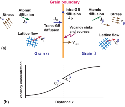
Figure 1: The physical processes occurring at the grain boundary and in the grains within the proposed model.

Consider two semi-infinite grains in a single-component solid. The grains are labeled $\alpha$ and $\beta$ and are separated by a planar GB (Fig. 1). The lattice site generation and annihilation process occurring at the GB causes rigid-body motion of the lattice of each grain toward or away from the GB. The grains can also translate past each other parallel to the GB plane by GB sliding or due to the shear-coupling effect (Cahn et al., 2006a, b). The respective velocities of the grains with respect to a chosen laboratory reference frame are denoted $\mathbf{v}_{L}^{\alpha}$ and $\mathbf{v}_{L}^{\beta}$, respectively. In addition to the rigid-body motion, atoms in the grains can diffuse through the lattice by the vacancy mechanism. The atomic diffusion fluxes relative to the reference frame attached to the lattices of the grains are $\mathbf{J}_{L}^{\alpha}$ and $\mathbf{J}_{L}^{\beta}$, respectively. Atoms can also diffuse along and across the moving GB. The respective diffusion fluxes measured relative to the GB structure are $\mathbf{J}_{b}$ and $\mathbf{J}_{n}=J_{n}\mathbf{n}^{\alpha}$, where $\mathbf{n}^{\alpha}$ is the unit normal vector pointing from grain $\alpha$ into grain $\beta$. The two-dimensional diffusion flux $\mathbf{J}_{b}$ measures the number of atoms in the GB plane crossing a unit GB length per unit time.

The entire bicrystal is subject to an applied mechanical stress. The elastic stresses arising inside the grains are represented by two Cauchy stress tensors $\mathbf{\boldsymbol{\sigma}_{\alpha}}$ and $\mathbf{\boldsymbol{\sigma}_{\beta}}$, respectively.

Thermodynamic properties of the interior regions of the grains are described by the grand-canonical potentials (per unit volume)

$$\omega_{\alpha}\equiv\dfrac{f_{s}^{\alpha}-M_{\alpha}c_{\alpha}}{\Omega_{\alpha}}$$ (1)

and

$$\omega_{\beta}\equiv\dfrac{f_{s}^{\beta}-M_{\beta}c_{\beta}}{\Omega_{\beta}},$$ (2)

where $f_{s}^{\alpha}$ and $f_{s}^{\beta}$ are the free energies per lattice site, $\Omega_{\alpha}$ and $\Omega_{\beta}$ are the respective atomic volumes, $M_{\alpha}=\partial f_{s}^{\alpha}/\partial c_{\alpha}$ and $M_{\beta}=\partial f_{s}^{\beta}/\partial c_{\beta}$ are the diffusion potentials of atoms relative to the vacancies, and $c_{\alpha}$ and $c_{\beta}$ are the atomic concentrations (fractions of occupied lattice sites) in the grains. The grand-canonical and diffusion potentials are functions of temperature, concentration and lattice strain relative to a chosen reference state. In this work, temperature is assumed to be uniform and permanently fixed.

Diffusion inside the grains follows the phenomenological equations (Mishin et al., 2015)

$$\mathbf{J}_{L}^{\alpha}=-L_{\alpha}\nabla M_{\alpha},$$ (3)

and

$$\mathbf{J}_{L}^{\beta}=-L_{\beta}\nabla M_{\beta},$$ (4)

respectively, where $L_{\alpha}>0$ and $L_{\beta}>0$ are diffusion kinetic coefficients. Combined with the mass conservation law, these equations describe the evolution of the atomic concentrations in space and time. Accordingly, the grand-canonical potentials, diffusion potentials and stresses are functions of the position vector $\mathbf{x}$ and time $t$.

For the description of GB processes, we will use the values of the aforementioned functions extrapolated toward the GB from either grain. The following notation is introduced for the extrapolated properties (Mishin et al., 2015). For any vector field $\mathbf{A}(\mathbf{x},t)$, let $\mathbf{A}_{\alpha}$ and $\mathbf{A}_{\beta}$ be the boundary values of $\mathbf{A}$ obtained by extrapolation from the grains $\alpha$ and $\beta$, respectively, at the same location. Then $\left[\mathbf{A}\right]\equiv\mathbf{A}_{\alpha}-\mathbf{A}_{\beta}$ represents the jump of $\mathbf{A}$ across the boundary and $\left\langle\mathbf{A}\right\rangle\equiv(\mathbf{A}_{\alpha}+\mathbf{A}_{\beta})/2$ is the average GB value of $\mathbf{A}$. Similar notations are used for scalar and tensor fields. In particular, diffusion of atoms across the boundary is described by the phenomenological equation

$$J_{n}=L_{t}\left[M\right],$$ (5)

while diffusion along the boundary by

$$\mathbf{J}_{b}=-L_{p}\nabla_{b}\left\langle M\right\rangle,$$ (6)

where $\nabla_{b}\left\langle M\right\rangle$ is the two-dimension gradient of $\left\langle M\right\rangle$ in the GB plane. In Eqs.(5) and (6), $L_{t}>0$ and $L_{p}>0$ are the kinetic coefficients for trans-boundary and intra-boundary diffusion, respectively (note that they have different dimensions).

The four diffusion fluxes $\mathbf{J}_{L}^{\alpha}$, $\mathbf{J}_{L}^{\beta}$, $\mathbf{J}_{b}$ and $\mathbf{J}_{n}$ are subject to two constraints. First, note that the number of atoms $\nu_{\alpha}$ added to grain $\alpha$ at the GB (per unit area per unit time) is

$$\nu_{\alpha}=\dfrac{c_{\alpha}}{\Omega_{\alpha}}\mathbf{n}^{\alpha}\mathbf{\cdot}\left(\mathbf{v}_{b}-\mathbf{v}_{L}^{\alpha}\right)-\mathbf{n}^{\alpha}\mathbf{\cdot}\mathbf{J}_{L}^{\alpha},$$ (7)

while the number of atoms added simultaneously to grain $\beta$ is

$$\nu_{\beta}=-\dfrac{c_{\beta}}{\Omega_{\beta}}\mathbf{n}^{\alpha}\mathbf{\cdot}\left(\mathbf{v}_{b}-\mathbf{v}_{L}^{\beta}\right)+\mathbf{n}^{\alpha}\mathbf{\cdot}\mathbf{J}_{L}^{\beta}.$$ (8)

Here, the dot denotes the inner product (contraction) of vectors or tensors and $\mathbf{v}_{b}$ is the GB velocity relative to the laboratory reference frame. The lattice velocities and lattice diffusion fluxes appearing in these equations are obtained by extrapolation to the GB from the respective grains. The atoms entering the GB from the grains can spread along it by GB diffusion. The conservation of atoms dictates that

$$\nu_{\alpha}+\nu_{\beta}=-\nabla_{b}\mathbf{\cdot}\mathbf{J}_{b},$$ (9)

where $\nabla_{b}\mathbf{\cdot}\mathbf{J}_{b}$ is the two-dimensional divergence of the GB flux $\mathbf{J}_{b}$. In addition, the normal diffusion flux across the GB can be expressed by (Mishin et al., 2015)

$$J_{n}=\dfrac{1}{2}(\nu_{\beta}-\nu_{\alpha}).$$ (10)

Equations (9) and (10) impose two constraints on the diffusion fluxes existing at the GB. They can be rewritten as

$$\left[\dfrac{c}{\Omega}\right]\mathbf{v}_{b}\mathbf{\cdot}\mathbf{n}^{\alpha}-\left[\dfrac{c}{\Omega}\mathbf{v}_{L}\right]\mathbf{\cdot}\mathbf{n}^{\alpha}-\left[\mathbf{J}_{L}\right]\mathbf{\cdot}\mathbf{n}^{\alpha}=-\nabla_{b}\mathbf{\cdot}\mathbf{J}_{b}$$ (11)

and

$$J_{n}=-\left\langle\dfrac{c}{\Omega}\right\rangle\mathbf{v}_{b}\mathbf{\cdot}\mathbf{n}^{\alpha}+\left\langle\dfrac{c}{\Omega}\mathbf{v}_{L}\right\rangle\mathbf{\cdot}\mathbf{n}^{\alpha}+\left\langle\mathbf{J}_{L}\right\rangle\mathbf{\cdot}\mathbf{n}^{\alpha},$$ (12)

respectively.

To formulate the site generation and GB migration equations, we decompose the lattice velocity jump $\left[\mathbf{v}_{L}\right]$ and the average lattice velocity $\left\langle\mathbf{v}_{L}\right\rangle$ into components normal and parallel to the GB: $\left[\mathbf{v}_{L}\right]=\left[\mathbf{v}_{L}\right]_{\bot}+\left[\mathbf{v}_{L}\right]_{||}$ and $\left\langle\mathbf{v}_{L}\right\rangle=\left\langle\mathbf{v}_{L}\right\rangle_{\bot}+\left\langle\mathbf{v}_{L}\right\rangle_{||}$. Similarly, for the GB traction vector $\mathbf{s}=\mathbf{n}^{\alpha}\mathbf{\cdot}\boldsymbol{\sigma}$ we have $\left\langle\mathbf{s}\right\rangle=\left\langle\mathbf{s}\right\rangle_{\bot}+\left\langle\mathbf{s}\right\rangle_{||}$ and $\left[\mathbf{s}\right]=\left[\mathbf{s}\right]_{\bot}+\left[\mathbf{s}\right]_{||}$. We will assume that the interiors of the grains and the GB itself remain in mechanical equilibrium at all times. This is a reasonable approximation if we focus the attention on relatively slow thermally-activated processes such as diffusion. Under mechanical equilibrium conditions, the traction vector is continuous across the GB plane, $\left[\mathbf{s}\right]_{\bot}=\left[\mathbf{s}\right]_{||}=\mathbf{0}$, and thus $\left\langle\mathbf{s}\right\rangle=\mathbf{s}$ (Mishin et al., 2015). It is assumed that the stress does not cause decohesion of the material, which would result in the formation of grain boundary cracks, pores and similar defects.

The normal component of the lattice velocity jump $\left[\mathbf{v}_{L}\right]_{\bot}$ is a measure of the site generation rate at the GB. As shown previously (Mishin et al., 2015), the thermodynamic driving force for the site generation at a planar GB is $\left\langle\omega\right\rangle-\mathbf{n}^{\alpha}\mathbf{\cdot}\mathbf{s}_{\bot}$. The term $\mathbf{n}^{\alpha}\mathbf{\cdot}\mathbf{s}_{\bot}$ captures the effect of the normal GB stress on the vacancy creation and annihilation process. The kinetic equation of this process can be written in the form

$$\mathbf{n}^{\alpha}\mathbf{\cdot}\left[\mathbf{v}_{L}\right]_{\bot}=R\left(\left\langle\omega\right\rangle-\mathbf{n}^{\alpha}\mathbf{\cdot}\mathbf{s}_{\bot}\right),$$ (13)

where $R>0$ is the respective kinetic coefficient. This coefficient controls the ability of the GB to absorb or generate vacancies. By contrast to some of the earlier models, we do not assume that the GB is a “perfect” sink/source of vacancies. By varying the parameter $R$ one can model GBs with a poor sink/source efficiency (small $R$) and with nearly ideal efficiency (large $R$). Based on the general knowledge of GBs (Sutton and Balluffi, 1995) and recent simulations (Gu et al., 2017), it is expected that the sink/source efficiency depends on the GB structure, crystallographic parameters, local chemistry and other factors.

Finally, the GB motion is driven by the grand-canonical potential jump $\left[\omega\right]$ and the shear stress $\left\langle\mathbf{s}\right\rangle_{||}$ parallel to the GB plane. The kinetic law of GB motion is (Mishin et al., 2015)

$$v_{GB}=-L_{GB}\left(\left[\omega\right]+\beta\left|\left\langle\mathbf{s}\right\rangle_{||}\right|\right),$$ (14)

where the kinetic coefficient $L_{GB}>0$ represents the GB mobility and $v_{GB}=\mathbf{n}^{\alpha}\mathbf{\cdot}\mathbf{v}_{b}-\mathbf{n}^{\alpha}\mathbf{\cdot}\left\langle\mathbf{v}_{L}\right\rangle$ is the GB migration velocity. The latter describes the GB motion relative to the lattices of the grains and is independent of the choice of the reference frame. In Eq.(14), the second term in the driving force arises from the shear-coupling effect (Cahn et al., 2006a, b). It is assumed that there is a certain direction in the boundary plane, defined by a unit vector $\mathbf{t}$, such that application of the shear stress $\left\langle\mathbf{s}\right\rangle_{||}$ parallel to that direction causes normal GB motion with a speed proportional to $\left\langle\mathbf{s}\right\rangle_{||}\cdot\mathbf{\mathbf{t}}$. Conversely, normal GB motion causes relative translation of the grains with a velocity $\left[\mathbf{v}_{L}\right]_{||}$ parallel to $\mathbf{t}$. The shear-coupling effect is described by the equation $\left[\mathbf{v}_{L}\right]_{||}\mathbf{\cdot\mathbf{t}}=\beta v_{GB}$, where the coupling factor $\beta$ depends on the crystallographic characteristics of the GB (Cahn et al., 2006a, b). The coupling factor is not unique to a given GB. It can change with temperature, direction of the shear stress and other factors as discussed in more detail in the recent literature (Han et al., 2018). It can also vary in time as the grain boundary structure changes due to the absorption or emission of vacancies (Borovikov et al., 2013). Some GBs respond to applied shear stresses by rigid sliding of the grains relative to each other. For such GBs, called uncoupled, the second term in the right-hand side of Eq.(14) vanishes. Instead, the mechanical response of the boundary to applied shear is described by a sliding law

$$\left[\mathbf{v}_{L}\right]_{||}=K_{s}\left\langle\mathbf{s}\right\rangle_{||},$$ (15)

where $K_{s}>0$ is the sliding coefficient. The GB migration is then solely driven by the jump $\left[\omega\right]$. Some GBs that are coupled at low temperatures can switch from coupling to sliding as temperature increases (Cahn et al., 2006b).

II.2 Specific model of a bicrystal

We will next specialize the above equations for a particular case when the vacancy concentration is small and the elastic deformations in the grains can be treated in the small-strain approximation (Mishin et al., 2015). As the reference state of the small-strain tensor $\boldsymbol{\varepsilon}$ we choose the stress-free solid without vacancies ($c=1$). The vacancies produce an isotropic stress-free deformation

$$\boldsymbol{\varepsilon}^{0}=\dfrac{\Delta\Omega_{v}}{3\Omega^{\prime}}\left(1-c\right)\mathbf{I},$$ (16)

where $\mathbf{I}$ is a $3\times 3$ unit tensor, $\Omega^{\prime}$ is the atomic volume in the reference state, and $\Delta\Omega_{v}<0$ is the vacancy relaxation volume under zero stress conditions. The total lattice strain is

$$\boldsymbol{\varepsilon}=\boldsymbol{\varepsilon}^{0}+\mathbf{S}:\boldsymbol{\sigma},$$ (17)

where $\mathbf{S}$ is the rank-four tensor of elastic compliances (the double-dot contraction of two second-rank tensors $\mathbf{a}$ and $\mathbf{b}$ is defined by $\mathbf{a}:\mathbf{b}=\textrm{Tr}(\mathbf{a}\mathbf{b}^{T})$ ).

Thermodynamic integration gives the following expressions for the grand-canonical and diffusion potentials inside the grains (Mishin et al., 2015):

$$\omega=\dfrac{1}{\Omega}\left(kT\ln\dfrac{1-c}{1-c^{*}}-\Delta\Omega_{v}c\sigma_{h}+\dfrac{\Omega^{\prime}}{2}\boldsymbol{\sigma}:\mathbf{S}:\boldsymbol{\sigma}\right),$$ (18)

$$M=M^{*}+kT\ln\dfrac{c(1-c^{*})}{c^{*}(1-c)}+\Delta\Omega_{v}\sigma_{h}.$$ (19)

Here, $c^{*}$ is the equilibrium atomic concentration in stress-free grains, $M^{*}$ is the respective equilibrium diffusion potential, $\sigma_{h}=\mathrm{Tr}(\boldsymbol{\sigma})/3$ is the hydrostatic part of the stress tensor, and

$$\Omega=\Omega^{\prime}\left[1+\mathrm{Tr}(\boldsymbol{\varepsilon})\right]=\Omega^{\prime}\left[1+\dfrac{\Delta\Omega_{v}}{\Omega^{\prime}}\left(1-c\right)\right]$$ (20)

is the atomic volume. In the latter equation, the term $\mathrm{Tr}(\mathbf{S}:\boldsymbol{\sigma})$ has been neglected due to the small-strain approximation of the elastic deformation.

We next take into account that the vacancy concentration $c_{v}\equiv(1-c)$ is very small ($c_{v}\ll 1$). Accordingly, all equations can be reformulated in terms of the small parameter $c_{v}$ and simplified. Equations (18) and (19) become

$$\omega=\dfrac{kT}{\Omega^{\prime}}\ln\dfrac{c_{v}}{c_{v}^{*}}-\dfrac{\Delta\Omega_{v}}{\Omega^{\prime}}\sigma_{h},$$ (21)

$$M=M^{*}-kT\ln\dfrac{c_{v}}{c_{v}^{*}}+\Delta\Omega_{v}\sigma_{h},$$ (22)

where $c_{v}^{*}=1-c^{*}$ is the equilibrium vacancy concentration in the absence of stresses. Note that we have neglected the term $\Delta\Omega_{v}c_{v}/\Omega^{\prime}$ in Eq.(20) in comparison with unity.

Using the diffusion potential from Eq.(22), the lattice diffusion equations (3) and (4) take the form

$$\mathbf{J}_{L}=D\dfrac{c_{v}}{\Omega^{\prime}c_{v}^{*}}\nabla c_{v}-D\dfrac{\Delta\Omega_{v}c_{v}^{2}}{\Omega^{\prime}kTc_{v}^{*}}\nabla\sigma_{h},$$ (23)

where $D$ is the diffusion coefficient in stress-free grains with the equilibrium vacancy concentration. Equation (23) was derived in our previous work (Mishin et al., 2015) by establishing a relation between the kinetic coefficients $L_{\alpha}$ and $L_{\beta}$ and the diffusion coefficient $D$ by the vacancy mechanism:

$$D=\dfrac{L_{\alpha}kT\Omega c_{v}^{*}}{c_{v}^{2}}$$ (24)

(and similarly for $L_{\beta}$). The first term in Eq.(23) represents the usual concentration-gradient driving force for vacancy diffusion, whereas the second term captures the stress-gradient effect. Since we assume that the grains do not contain sinks or sources of vacancies, the continuity equation can be applied, leading to the diffusion equation

$$\dfrac{\partial c_{v}}{\partial t} = \dfrac{Dc_{v}}{c_{v}^{*}}\nabla^{2}c_{v}+\dfrac{D}{c_{v}^{*}}\left(\nabla c_{v}\right)^{2}-\mathbf{v}_{L}\mathbf{\cdot}\nabla c_{v}$$ (25)

$$- \dfrac{D\Delta\Omega_{v}}{kTc_{v}^{*}}c_{v}^{2}\nabla^{2}\sigma_{h}-\dfrac{2D\Delta\Omega_{v}}{kTc_{v}^{*}}c_{v}\nabla\sigma_{h}\cdot\nabla c_{v}.$$

The site generation and GB migration equations (13) and (14) include the discontinuity and the average value of the grand-canonical potential. To simplify the calculations, we will assume that the hydrostatic stress is continuous across the boundary. This assumption is more strict than the mechanical equilibrium conditions alone, which only requires that the traction vector be continuous. Under this assumption,

$$\left[\omega\right]=\dfrac{kT}{2\Omega^{\prime}}\ln\dfrac{c_{v}^{\alpha}}{c_{v}^{\beta}},$$ (26)

$$\left\langle\omega\right\rangle=\dfrac{kT}{2\Omega^{\prime}}\ln\dfrac{c_{v}^{\alpha}c_{v}^{\beta}}{\left(c_{v}^{*}\right)^{2}}-\dfrac{\Delta\Omega_{v}\sigma_{h}}{\Omega^{\prime}}.$$ (27)

In these equations, $c_{v}^{\alpha}$ and $c_{v}^{\beta}$ are the GB values of the vacancy concentration extrapolated from the grains. Similarly, $\left[M\right]$ and $\left\langle M\right\rangle$ appearing in the trans-boundary and intra-boundary diffusion equations are given by

$$\left[M\right]=-\dfrac{kT}{2}\ln\dfrac{c_{v}^{\alpha}}{c_{v}^{\beta}},$$ (28)

$$\left\langle M\right\rangle=M^{*}-\dfrac{kT}{2}\ln\dfrac{c_{v}^{\alpha}c_{v}^{\beta}}{\left(c_{v}^{*}\right)^{2}}+\Delta\Omega_{v}\sigma_{h}.$$ (29)

III Numerical study

III.1 The governing equations

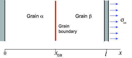
Figure 2: Schematic bicrystal with a plane grain boundary. The left bar indicates the fixed wall. The system is subject to uniform uniaxial stress $\sigma_{xx}$ in the $x$-direction.

The following case is chosen for a parametric numerical study. Suppose the grains $\alpha$ and $\beta$ are separated by a plane incoherent GB normal to the Cartesian direction $x$ (Fig. 2). At the left end, the grain $\alpha$ is attached to a fixed wall at $x=0$. The reference frame is also attached to the wall. At the right end, the grain $\beta$ terminates at a movable wall (piston) capable of exerting a prescribed normal stress $\sigma_{11}$ without shear ($\sigma_{12}=\sigma_{13}=0$). Let $x_{GB}(t)$ denote the current GB position and $x=l(t)$ be the right end of grain $\beta$. The lateral dimensions of the grains are assumed to be much larger than $l$. All intensive properties of the system depend only on the coordinate $x$, making the problem effectively one-dimensional. The temperature is fixed.

Suppose the lateral dimensions of the system were initially adjusted so that in the absence of the external force ($\sigma_{11}=0$), the system reached thermodynamic equilibrium with stress-free grains. The equilibrium vacancy concentration in this state is $c_{v}^{*}$. The lateral dimensions of the grains were then fixed once and for all. Next, the vacancy concentration was modified (e.g., by irradiation) and/or a stress $\sigma_{11}$ was applied. This creates a new initial state whose subsequent evolution we wish to investigate. Note that during this evolution, the boundary conditions ensure that the lateral lattice strains, $\varepsilon_{22}$ and $\varepsilon_{33}$, remain fixed at the initial, stress-free value [cf. Eq.(16)],

$$\varepsilon_{22}=\varepsilon_{33}=\dfrac{\Delta\Omega_{v}}{3\Omega^{\prime}}c_{v}^{*}.$$ (30)

To simplify the calculations, the grains will be treated as homogeneous, elastically isotropic media with a Young modulus $E$ and Poisson’s factor $\nu$. As before, it is assumed that mechanical equilibrium is always maintained ($\nabla\cdot\boldsymbol{\sigma}=\mathbf{0}$). Consequently, $\sigma_{22}$ and $\sigma_{33}$ must be equal functions of only $x$ ($\sigma_{22}(x)=\sigma_{33}(x)$), $\sigma_{11}$ must be uniform throughout the system and equal to its boundary value at $x=l$, and all other stress components must be zero. Furthermore, as was done above, we will neglect the stress-free strain produced by the vacancies. In this approximation $\varepsilon_{22}=\varepsilon_{33}=0$ and the isotropic Hooke’s law is readily solved for the normal strain $\varepsilon_{11}$ and lateral stresses $\sigma_{22}$ and $\sigma_{33}$:

$$\varepsilon_{11}=\dfrac{(1+\nu)(1-2\nu)}{E(1-\nu)}\sigma_{11},$$ (31)

$$\sigma_{22}=\sigma_{33}=\dfrac{\nu}{1-\nu}\sigma_{11}.$$ (32)

Thus, all stresses and strains in the system are uniform, time-independent, and are uniquely defined by the applied normal stress $\sigma_{11}$. The hydrostatic part of the stress tensor is

$$\sigma_{h}=\dfrac{1}{3}\left(\dfrac{1+\nu}{1-\nu}\right)\sigma_{11}.$$ (33)

The lattice velocity field $v_{L}(x,t)$ is generally related to the deformation rate by $\partial v_{L}/\partial x=\dot{\varepsilon}_{11}$. However, due to the neglect of the stress-free strain, $\varepsilon_{11}$ is constant and thus $\partial v_{L}/\partial x=0$. Each grain moves with a uniform velocity as a rigid body. Because grain $\alpha$ is attached to the wall, its velocity vanishes, while grain $\beta$ moves with a time-dependent velocity $v_{L}^{\beta}(t)$.

Diffusion inside the grains is described by Eqs.(23) and (25), which simplify to

$$J_{L}=\dfrac{Dc_{v}}{\Omega^{\prime}c_{v}^{*}}\dfrac{\partial c_{v}}{\partial x}$$ (34)

and

$$\dfrac{\partial c_{v}}{\partial t}=\dfrac{Dc_{v}}{c_{v}^{*}}\dfrac{\partial^{2}c_{v}}{\partial x^{2}}+\dfrac{D}{c_{v}^{*}}\left(\dfrac{\partial c_{v}}{\partial x}\right)^{2}-v_{L}\dfrac{\partial c_{v}}{\partial x},$$ (35)

respectively. Note that the stress derivatives appearing in Eqs.(23) and (25) have vanished due to the spatial uniformity of the stress tensor.

Turning to GB processes, the axial symmetry of the problem precludes lateral diffusion in the GB. Thus $\mathbf{J}_{b}=\mathbf{0}$ and the mass conservation equation (11) takes the form

$$\left(c_{v}^{\beta}-c_{v}^{\alpha}\right)\dfrac{dx_{GB}}{dt}+v_{L}^{\beta}+\dfrac{D}{c_{v}^{*}}\left(c_{v}^{\beta}\left(\dfrac{\partial c_{v}}{\partial x}\right)_{\beta}-c_{v}^{\alpha}\left(\dfrac{\partial c_{v}}{\partial x}\right)_{\alpha}\right)=0.$$ (36)

Note that in the second term we replaced $c_{\beta}v_{L}^{\beta}$ by $v_{L}^{\beta}$ due to the smallness of the vacancy concentration. The normal flux of atoms across the boundary is

$$J_{n}=-\dfrac{1}{\Omega^{\prime}}\dfrac{dx_{GB}}{dt}+\dfrac{v_{L}^{\beta}}{2\Omega^{\prime}}+\dfrac{D}{2c_{v}^{*}\Omega^{\prime}}\left(c_{v}^{\alpha}\left(\dfrac{\partial c_{v}}{\partial x}\right)_{\alpha}+c_{v}^{\beta}\left(\dfrac{\partial c_{v}}{\partial x}\right)_{\beta}\right),$$ (37)

where we have used Eq.(12) and approximated $c_{\alpha}+c_{\beta}\approx 2$ and $c_{\beta}\approx 1$. Using $\left[M\right]$ from Eq.(28), the kinetic equation of trans-boundary diffusion (5) becomes

$$-2\dfrac{dx_{GB}}{dt}+v_{L}^{\beta}+\dfrac{D}{c_{v}^{*}}\left(c_{v}^{\alpha}\left(\dfrac{\partial c_{v}}{\partial x}\right)_{\alpha}+c_{v}^{\beta}\left(\dfrac{\partial c_{v}}{\partial x}\right)_{\beta}\right)=-L_{t}^{\prime}\ln\dfrac{c_{v}^{\alpha}}{c_{v}^{\beta}}$$ (38)

with the kinetic coefficient $L_{t}^{\prime}=kT\Omega^{\prime}L_{t}$. The vacancy generation equation (13) simplifies to

$$v_{L}^{\beta}=-R\left(\left\langle\omega\right\rangle-\sigma_{11}\right),$$ (39)

while the GB migration equation (14) reduces to

$$v_{GB}=\dfrac{dx_{GB}}{dt}-\dfrac{1}{2}v_{L}^{\beta}=-L_{GB}\left[\omega\right].$$ (40)

Equations (39) and (40) show that, under vacancy equilibrium conditions, $\omega$ must be uniform throughout the system and equal to $\sigma_{11}$. The equilibrium vacancy concentration $c_{v}^{eq}$ must be also uniform and satisfy the equation

$$\dfrac{kT}{\Omega^{\prime}}\ln\dfrac{c_{v}^{eq}}{c_{v}^{*}}=\dfrac{\Delta\Omega_{v}}{\Omega^{\prime}}\sigma_{h}+\sigma_{11},$$ (41)

where we used Eq.(27) for $\left\langle\omega\right\rangle$. When $\sigma_{11}=0$, $c_{v}^{eq}$ reduces to its stress-free value $c_{v}^{*}$.

If the term with $\Delta\Omega_{v}$ could be dropped, Eq.(41) would reduce to Herring’s relation for the effect of applied stress on the vacancy concentration in solids (Herring, 1949, 1950). However, this term is generally non-negligible since $\Delta\Omega_{v}$ is usually not much smaller than $\Omega^{\prime}$. This term captures the additional effect of lateral elastic deformation on the equilibrium vacancy concentration in stressed solids. In the bicrystal considered here, the lateral stresses arise due to the constraint opposing the Poisson deformation caused by the normal stress. We note in passing that in other cases lateral stresses can be more significant. In epitaxial thin films, lateral (in-plane) stresses can be high while $\sigma_{11}$ is zero, or at least much smaller. Under such conditions, it is the lateral stress that dictates the vacancy concentration in the film.

In the final form, the vacancy generation and GB migration equations take the forms

$$v_{L}^{\beta}=-\dfrac{RkT}{2\Omega^{\prime}}\ln\dfrac{c_{v}^{\alpha}c_{v}^{\beta}}{\left(c_{v}^{eq}\right)^{2}}$$ (42)

and

$$\dfrac{dx_{GB}}{dt}-\dfrac{1}{2}v_{L}^{\beta}=-\dfrac{kTL_{GB}}{2\Omega^{\prime}}\ln\dfrac{c_{v}^{\alpha}}{c_{v}^{\beta}},$$ (43)

respectively.

III.2 The numerical method for solving the equations

The kinetic equations formulated above form a closed system that can be solved numerically as follows. The diffusion equation (35) is solved inside each grain individually, with $v_{L}^{\alpha}\equiv 0$ in grain $\alpha$ and the instantaneous lattice velocity $v_{L}^{\beta}(t)$ in grain $\beta$. Note that both equations must be solved in domains with moving boundaries. At $x=0$ and $x=l(t)$, the zero-flux conditions $\partial c_{v}/\partial x\equiv 0$ are applied. We need two more boundary conditions at the GB and must know the velocities $v_{L}^{\beta}$ and $\dot{x}_{GB}$. This information is provided by the four equations (36), (38), (42) and (43). The initial condition for the vacancy concentration can be chosen arbitrarily. We thus need to solve a system of partial differential equations in two variable-size domains simultaneously with differential equations describing the boundary conditions at the moving interfaces. Similar equations often arise when describing the dynamics of solidification, phase precipitation, and other processes involving a phase formation. In the present case, both grains represent the same phase but have variable dimensions due to the grain boundary motion and the lattice site formation and annihilation at the boundary.

Numerical simulations were performed using an explicit-in-time finite difference approximation to the differential equations, coupled to a nonlinear solver that treats the interface conditions implicitly. More specifically, the spatial domains $0<x<x_{GB}(t)$ and $x_{GB}(t)<x<l(t)$ were mapped to fixed computational domains $0<z<1$ and $1<z<2$, respectively, via the transformations

$$z=\dfrac{x}{x_{GB}(t)},\qquad x<x_{GB}(t),$$ (44)

$$z=1+\dfrac{x-x_{GB}(t)}{l(t)-x_{GB}(t)},\qquad l(t)>x>x_{GB}(t),$$ (45)

which result in a new set of differential equations that explicitly involve coefficients that depend on $x_{GB}(t)$ and $l(t)$. Given the solution at time $t=n\Delta t$, the vacancy concentration field at time $t=(n+1)\Delta t$ was computed at interior points of the grains (excluding the GB) by using a first-order-accurate explicit time differencing scheme (“forward Euler method”), together with no-flux boundary conditions at the sample ends. To complete the solution at this time step, the four additional unknowns $c_{v}^{\alpha}$, $c_{v}^{\beta}$, $v_{L}^{\beta}$ and $dx_{GB}/dt$ were solved by applying Newton’s method to the four equations (36), (38), (42) and (43). The derivatives $\left(\partial c_{v}/\partial x\right)_{\alpha}$ and $\left(\partial c_{v}/\partial x\right)_{\beta}$ appearing in Eqs.(36) and (38) are evaluated using one-sided derivatives using the latest interior values of the vacancy concentration. Good initial guesses for the nonlinear solver are available from the previous time step. Given the updated velocities of the lattice and the GB, new values of $l(t)$ and $x_{GB}(t)$ were obtained by again using a first-order time difference to complete the solution at the new time level. Numerical stability considerations restrict the size of the time step $\Delta t$ to scale with the square of the spatial mesh, but this is not a serious limitation in one spatial dimension. For numerical convenience, in all calculations reported below, the equilibrium vacancy concentration is $c_{v}^{*}=10^{-4}$. For comparison, in most materials the vacancy concentration near the melting point ranges from $10^{-3}$ to $10^{-5}$ (Kraftmakher, 1998).

III.3 Dimensionless form of the governing equations

The numerical results will be analyzed in terms of the following dimensionless variables: time $\tau=Dt/l_{0}^{2}$, coordinate $\xi=x/l_{0}$, the system length $\xi_{l}=l/l_{0}$, the GB position $\xi_{GB}=x_{GB}/l_{0}$, the lattice velocity $\eta=v_{L}^{\beta}l_{0}/D$, the stress $s=\sigma_{11}\Omega^{\prime}/kT$, and the normalized vacancy concentration $C=c_{v}/c_{v}^{*}$, where $l_{0}$ is the initial length of the bicrystal. The dimensionless GB velocity is

$$\eta_{GB}=\dfrac{v_{GB}l_{0}}{D}=\dfrac{d\xi_{GB}}{d\tau}-\dfrac{\eta}{2}.$$ (46)

The dimensionless diffusion equations of the model become

$$\dfrac{\partial C}{\partial\tau}=C\dfrac{\partial^{2}C}{\partial\xi^{2}}+\left(\dfrac{\partial C}{\partial\xi}\right)^{2},\>\>\>\mathrm{grain\>\alpha},$$ (47)

$$\dfrac{\partial C}{\partial\tau}=C\dfrac{\partial^{2}C}{\partial\xi^{2}}+\left(\dfrac{\partial C}{\partial\xi}\right)^{2}-\eta\dfrac{\partial C}{\partial\xi},\>\>\>\mathrm{grain\>\beta}.$$ (48)

The vacancy concentration fields in the grains are subject to the boundary conditions $\partial C/\partial\xi\equiv 0$ at $\xi=0$ and $\xi=\xi_{l}(t)$, and to the following boundary equations at $\xi=\xi_{GB}(t)$:

$$-2\dfrac{d\xi_{GB}}{d\tau}+\eta+c_{v}^{*}\left(C_{\alpha}\left(\dfrac{\partial C}{\partial\xi}\right)_{\alpha}+C_{\beta}\left(\dfrac{\partial C}{\partial\xi}\right)_{\beta}\right)=-\lambda_{t}\ln\dfrac{C_{\alpha}}{C_{\beta}},$$ (49)

$$c_{v}^{*}\left(C_{\beta}-C_{\alpha}\right)\dfrac{d\xi_{GB}}{d\tau}+\eta+c_{v}^{*}\left(C_{\beta}\left(\dfrac{\partial C}{\partial\xi}\right)_{\beta}-C_{\alpha}\left(\dfrac{\partial C}{\partial\xi}\right)_{\alpha}\right)=0,$$ (50)

$$\eta=-\rho\left(\dfrac{1}{2}\ln C_{\alpha}C_{\beta}-\dfrac{b}{3}\left(\dfrac{1+\nu}{1-\nu}\right)s-s\right),$$ (51)

$$\dfrac{d\xi_{GB}}{d\tau}=\dfrac{1}{2}\eta-\lambda\ln\dfrac{C_{\alpha}}{C_{\beta}}.$$ (52)

These equations depend on the dimensionless parameters $\lambda_{t}=(l_{0}/D)L_{t}^{\prime}$, $\lambda=(kTl_{0}/D\Omega^{\prime})L_{GB}$, $\rho=(kTl_{0}/D\Omega^{\prime})R$ and $b=\Delta\Omega_{v}/\Omega^{\prime}$. These parameters control the trans-boundary diffusion, the GB mobility, the rate of vacancy generation/annihilation at the GB, and the vacancy relaxation volume, respectively.

Note that $\xi_{l}(0)=1$ by definition. At any moment of time, the current length of the sample can be found by the integration

$$\xi_{l}(\tau)=1+\intop_{0}^{\tau}\eta(\tau)d\tau.$$ (53)

The evolution of the system depends on the initial vacancy distribution $C(\xi,0)$ in each grain, the initial GB position $\xi_{GB}(0)$, and the applied stress $s$. The system eventually reaches equilibrium with a stress-dependent uniform vacancy concentration $c_{v}^{eq}$. The latter can be obtained from Eq.(51) by setting $\eta=0$, which gives

$$\ln C^{eq}\equiv\ln\dfrac{c_{v}^{eq}}{c_{v}^{*}}=\left(1+\dfrac{b}{3}\left(\dfrac{1+\nu}{1-\nu}\right)\right)s.$$ (54)

Without loss of generality, we will assume that $s=0$ and thus $C^{eq}=1$. Under this condition, the dynamics are only driven by diffusive redistribution of the vacancies between the grains and absorption of non-equilibrium vacancies by the grain boundary. For nonzero stress, the solution can be readily obtained by redefining the dimensionless vacancy concentration as $C=c_{v}/c_{v}^{eq}$, where $c_{v}^{eq}$ refers to the equilibrium state under $s\neq 0$. The evolution equations are then obtained by simply replacing $c_{v}^{*}$ by $c_{v}^{eq}$ and re-interpreting $D$ as the diffusion coefficient in the stressed lattice with the vacancy concentration $c_{v}^{eq}$.

III.4 The normal modes of relaxation

The linear stability analysis of the model presented in Appendix B shows that there are two non-trivial relaxation modes near the system equilibrium. The linear stability analysis assumes that the GB and lattice velocities and the deviation of the vacancy concentration from equilibrium all decay with time in proportion to $\exp(-\kappa^{2}\tau)$. In the so-called $\kappa_{\rho}$ mode, the decaying solutions are (cf. Eq.(86))

$$C_{\alpha}=1+\hat{C}\exp(-\kappa_{\rho}^{2}\tau)\cos\xi\kappa_{\rho},$$ (55)

$$C_{\beta}=1+\hat{C}\exp(-\kappa_{\rho}^{2}\tau)\cos(\xi-1)\kappa_{\rho},$$ (56)

$$\xi_{GB}=\dfrac{1}{2}+\dfrac{\rho\hat{C}}{2\kappa_{\rho}^{2}}\exp(-\kappa_{\rho}^{2}\tau)\cos\dfrac{\kappa_{\rho}}{2},$$ (57)

$$\eta=-\rho\hat{C}\exp(-\kappa_{\rho}^{2}\tau)\cos\dfrac{\kappa_{\rho}}{2}.$$ (58)

Here, $\hat{C}$ is the initial excess of the vacancy concentration over the equilibrium value at the ends of the sample. The boundary is initially at $\xi=1/2$, where the vacancy excess is $\hat{C}\cos\kappa_{\rho}/2$. The wavenumber $\kappa_{\rho}$ is the root of the transcendental equation

$$\dfrac{2Z_{\rho}}{\kappa_{\rho}}=\tan\dfrac{\kappa_{\rho}}{2},$$ (59)

with the constant parameter

$$Z_{\rho}=\dfrac{\rho}{4c_{v}^{*}}.$$ (60)

In this mode, the vacancy concentration is a continuous (no interface gap) and even function about the GB position. The dominant relaxation process is the vacancy generation or absorption by the GB. The boundary itself does not move relative to the mean velocity of the grains ($\eta_{GB}=d\xi_{GB}/d\tau-\eta/2=0$).

The second normal mode is referred to as the $\kappa_{\lambda}$ mode, in which (cf. Eq.(89))

$$C_{\alpha}=1+\hat{C}\exp(-\kappa_{\lambda}^{2}\tau)\cos\xi\kappa_{\lambda},$$ (61)

$$C_{\beta}=1-\hat{C}\exp(-\kappa_{\lambda}^{2}\tau)\cos(\xi-1)\kappa_{\lambda},$$ (62)

$$\xi_{GB}=\dfrac{1}{2}+\dfrac{2\lambda\hat{C}}{\kappa_{\lambda}^{2}}\exp(-\kappa_{\lambda}^{2}\tau)\cos\dfrac{\kappa_{\lambda}}{2},$$ (63)

$$\eta=0,$$ (64)

where $\kappa_{\lambda}$ is the root of the equation

$$\dfrac{2Z_{\lambda}}{\kappa_{\lambda}}=\tan\dfrac{\kappa_{\lambda}}{2},$$ (65)

with

$$Z_{\lambda}=\dfrac{2\lambda+\lambda_{t}}{2c_{v}^{*}}.$$ (66)

There is no vacancy generation or absorption at the boundary. The relaxation occurs by vacancy diffusion in the grains and across the GB. The initial vacancy concentration is $1+\hat{C}$ at $\xi=0$ and $1-\hat{C}$ at $\xi=1$. Thus, the vacancies are oversaturated at one end of the sample and undersaturated at the other. The vacancy concentration profile is an odd function relative to the GB position, with the concentration gap

$$\Delta C=C_{\beta}-C_{\alpha}=\hat{C}\exp(-\kappa_{\lambda}^{2}\tau)\cos\dfrac{\kappa_{\lambda}}{2}$$

at the boundary. During the relaxation process, the concentration gap narrows down and eventually vanishes as the vacancy concentration reaches the equilibrium value $C_{\beta}=C_{\alpha}=1$. Note that this process is accompanied by GB migration with the velocity

$$\eta_{GB}=\dfrac{d\xi_{GB}}{d\tau}=-2\lambda\Delta C$$

driven by the vacancy concentration gap $\Delta C$.

The present model contains three dimensionless kinetic coefficients: $\lambda$, $\lambda_{t}$ and $\rho$, which control the GB mobility, trans-boundary diffusion and vacancy generation/adsorption, respectively. The linear stability analysis identifies two combinations of these parameters, $Z_{\rho}$ and $Z_{\lambda}$, which can be the most effective predictors of the system evolution. Therefore, the numerical cases presented below were primarily chosen based on the values of $Z_{\rho}$ and $Z_{\lambda}$.

III.5 Numerical results

III.5.1 Relaxation modes

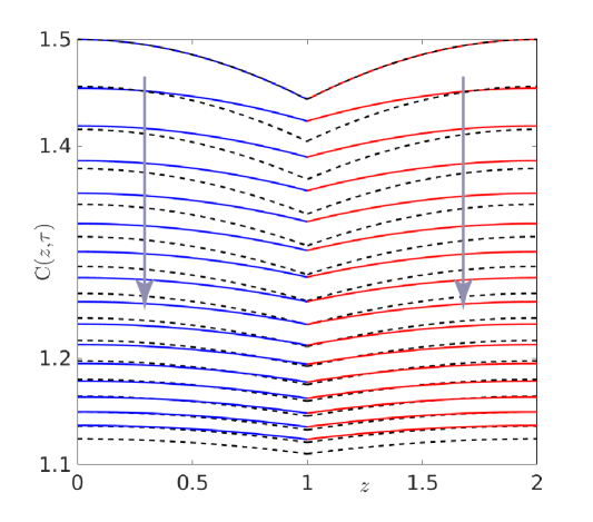
(b)  

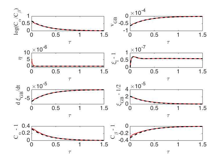
Figure 3: (a) Comparison of the $\kappa_{\rho}$ normal mode solution (dashed black curves) and the nonlinear numerical solution (solid blue and red curves) for the vacancy concentration fields in each grain. The concentration profiles are shown at times $\tau$ ranging from 0 to 1.5 at 0.1 increments. The arrows indicate the direction of time. The model parameters are $\lambda=\lambda_{t}=0$ and $\rho=10^{-4}$ (thus $Z_{\rho}=1/4$ and $Z_{\lambda}=0$) and the initial perturbation has the amplitude $\hat{C}=0.5$. (b) Comparison of the same normal mode solution (dashed red curves) and nonlinear numerical solution (solid black curves) for various interfacial quantities.

We will start by illustrating the two normal modes mentioned above. To create the $\kappa_{\rho}$ mode, we choose $\lambda=\lambda_{t}=0$ and $\rho=10^{-4}$. For these values of the parameters, we have $Z_{\rho}=1/4$ and $Z_{\lambda}=0$. The initial distribution is given by Eqs.(55) and (56) with $\tau=0$ and $\hat{C}=0.5$, so the maximum vacancy concentration in the system is $1.5c_{v}^{*}$. The GB velocity is initialized by $d\xi_{GB}/d\tau=0$. The vacancy concentration profiles obtained by numerical solution of Eqs.(47)-(52) are plotted as a function of time in Fig. 3. For comparison, the dashed lines show predictions of the normal mode equations (55) and (56). Since the grain sizes can vary in time, it is convenient to map the vacancy concentration profiles in the grains $\alpha$ and $\beta$ onto fixed-size intervals $[0,1]$ and $[1,2]$, respectively, by the coordinate transformations (cf. Eqs.(44) and (45))

$$z=\dfrac{\xi}{\xi_{GB}(\tau)},\qquad\xi<\xi_{GB}(\tau),$$ (67)

$$z=1+\dfrac{\xi-\xi_{GB}(\tau)}{\xi_{l}(\tau)-\xi_{GB}(\tau)},\qquad\xi_{l}(\tau)>\xi>\xi_{GB}(\tau).$$ (68)

This transformation was applied to all vacancy concentration plots shown in the paper. The functions $\xi_{GB}(\tau)$ and $\xi_{l}(\tau)$ are then plotted in separate panels.

The plots in Fig. 3(a) demonstrate the formation of a minimum in the vacancy concentration located at the GB, which approaches the equilibrium value causing the profile to become deeper and wider with time until the entire system reaches the vacancy equilibrium. The vacancy absorption at the boundary results in elimination of atomic layers on either side of the GB plane and thus shrinkage of both grains by equal amount, as illustrated in Fig. 3(b). The GB migration velocity relative to the grains remains zero within the numerical accuracy. Note the reasonable agreement between the numerical solution of the nonlinear model and the normal mode predictions. The differences between the two solutions arise from the fact that the normal mode only represents the asymptotic behavior in the limit of small deviations from equilibrium. Much closer agreement was found in a similar comparison for a small perturbation by $\hat{C}=0.5\times 10^{-4}$ (see Fig. 1 in the Supplementary Material (Sup, ????)).

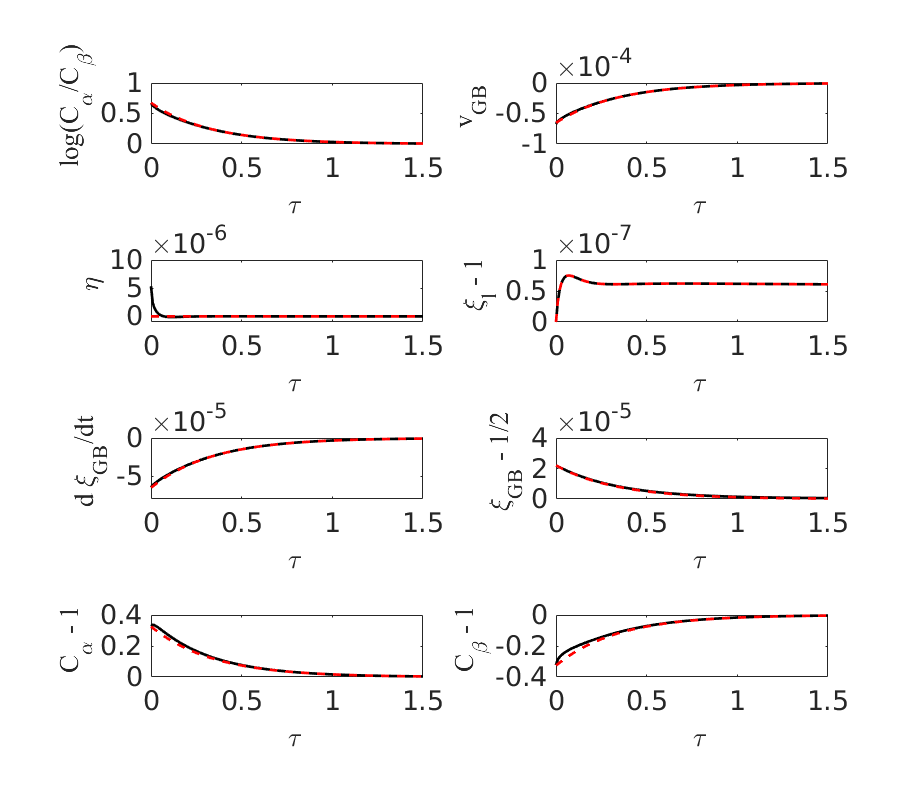
Figure 4: (a) Comparison of the $\kappa_{\lambda}$ normal mode solution (dashed black curves) and the nonlinear numerical solution (solid blue and red curves) for the vacancy concentration fields in each grain. The concentration profiles are shown at times $\tau$ ranging from 0 to 1.5 at 0.1 increments. The arrows indicate the direction of time. The model parameters are $\lambda=10^{-4}$, $\lambda_{t}=0$ and $\rho=10^{-4}$ (thus $Z_{\rho}=1/4$ and $Z_{\lambda}=1$). (b) Comparison of the same normal mode solution (dashed red curves) and nonlinear numerical solution (solid black curves) for various interfacial quantities.

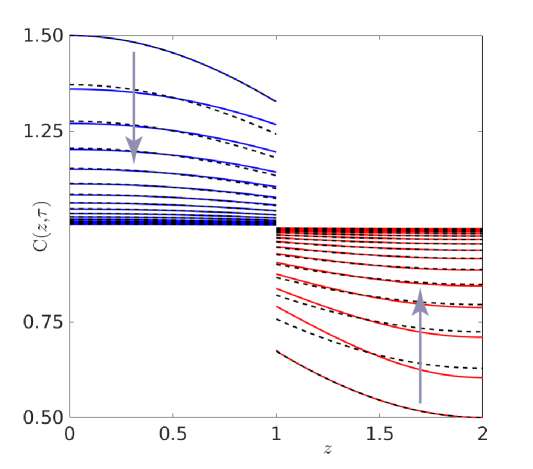
(b)  

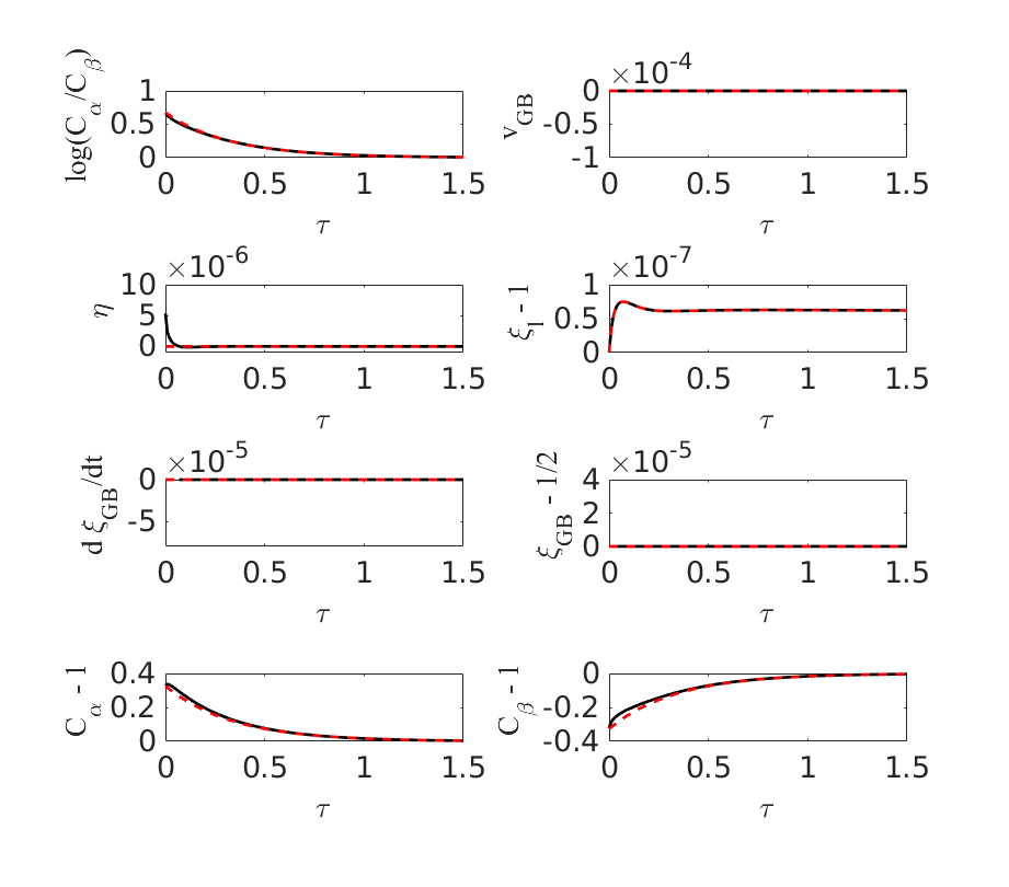
Figure 5: (a) Comparison of the $\kappa_{\lambda}$ normal mode solution (dashed black curves) and the nonlinear numerical solution (solid blue and red curves) for the vacancy concentration fields in each grain. The concentration profiles are shown at times $\tau$ ranging from 0 to 1.5 at 0.1 increments. The arrows indicate the direction of time. The model parameters are $\lambda=0$, $\lambda_{t}=2\times 10^{-4}$ and $\rho=10^{-4}$ (thus $Z_{\rho}=1/4$ and $Z_{\lambda}=1$). (b) Comparison of the same normal mode solution (dashed red curves) and nonlinear numerical solution (solid black curves) for various interfacial quantities.

The $\kappa_{\lambda}$ mode was implemented by creating the initial vacancy distribution according to Eqs.(61) and (62) with $\tau=0$ and $\hat{C}=0.5$ (Figs. 4 and 5). We again choose $\rho=10^{-4}$ and thus $Z_{\rho}=1/4$. The parameter $Z_{\lambda}$ depends on the combination $2\lambda+\lambda_{t}$. Instead of choosing one particular value of this combination, two different cases were tested, namely, $\lambda=10^{-4}$ and $\lambda_{t}=0$, and $\lambda=0$ and $2\times 10^{-4}$. Although both cases have the same $Z_{\lambda}=1$, the situations are physically different. In the first case, the GB is mobile while diffusion across the GB is prohibited. The excess vacancies diffuse from grain $\alpha$ toward the left-hand side of the boundary, where they are annihilated. By the symmetry of the equations, the right-hand side of the boundary simultaneously injects the same amount of vacancies into grain $\beta$. As a result, grain $\alpha$ shrinks while grain $\beta$ expands, keeping the same size of the system and zero lattice velocity in grain $\beta$ (Fig. 4). The GB migrates toward grain $\alpha$ while the vacancy concentration jump at the boundary decreases and eventually closes. In the second case, the vacancies diffuse across the GB, from grain $\alpha$ to grain $\beta$, which again results in reducing and eventually closing the concentration gap (Fig. 5). However, while there is a driving force for GB migration, the boundary does not move due to its zero mobility coefficient ($\lambda=0$). In both cases, the time evolution of the vacancy concentration is similar and relatively close to the respective normal mode solution (61)-(62). Similar tests with a small perturbation ($\hat{C}=0.5\times 10^{-4}$) show much closer agreement between the nonlinear model and the respective normal mode solution. (see Figs. 3 and 4 in the Supplementary Material (Sup, ????)). These calculations demonstrate that, in spite of the drastic difference in the $\lambda$ and $\lambda_{t}$ parameters and the operation of different physical mechanisms, the vacancy relaxation kinetics is in both cases similar and is primarily governed by the parameters $Z_{\rho}$ and $Z_{\lambda}$.

III.5.2 Mixed-mode cases

Further calculations were performed in the mixed-mode regime by creating an initial vacancy distribution different from that in either normal mode. Namely, the initial vacancy concentration profile was chosen to be

$$C_{\alpha}=1,\qquad 0\leq\xi\leq 1/2,$$ (69)

$$C_{\beta}=\dfrac{3}{2}+\dfrac{3}{4}\left(4\xi-3\right)-\dfrac{1}{4}\left(4\xi-3\right)^{3},\qquad 1/2\leq\xi\leq 1.$$ (70)

By these equations, the vacancy concentration is at equilibrium in grain $\alpha$ ($C_{\alpha}\equiv 1$), twice the equilibrium value at the right end of the sample ($C_{\beta}=2$ at $\xi=1$), and tends smoothly to the equilibrium value when approaching the GB from grain $\beta$. Since this function is neither even nor odd with respect to the GB position $\xi=1/2$, the vacancy relaxation process does not have to follow a particular normal mode. The vacancy concentration jump and concentration gradient at the boundary are initially zero.

Table 2 summarizes eight combinations of the dimensionless model parameters that were tested, where each parameter was taken to be either very large or very small. The orders of magnitude of these dimensionless parameters were chosen based on estimates of the possible ranges of the physical parameters on which they depend. The accompanying online Supplementary file (Sup, ????) contains a collection of the vacancy concentration profiles and various interface properties as functions of time for all eight cases. Four of the most representative cases will be discussed below.

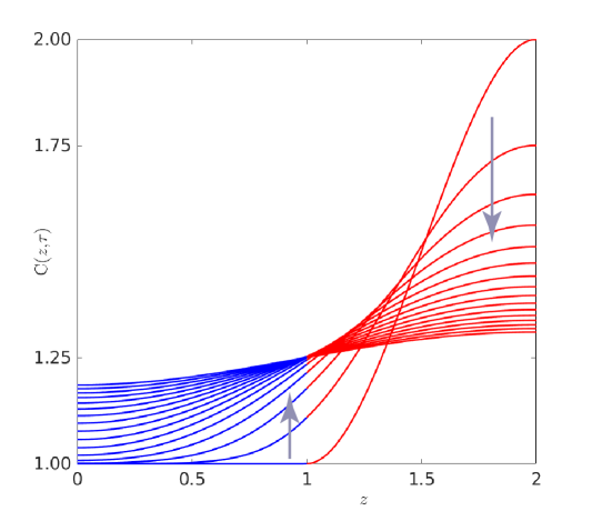
(b)  

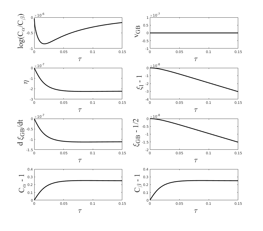
Figure 6: Vacancy concentration profiles (a) and various interfacial quantities. (b) obtained by numerical solution of the model. The concentration profiles are shown at times $\tau$ ranging from 0 to 1.5 at 0.1 increments. The arrows indicate the direction of time. The model parameters correspond to case 4 in Table 2.

In the first example, corresponding to case 4 in Table 2, $\lambda$ and $\rho$ are chosen to be small, meaning that the GB is highly immobile and virtually incapable of vacancy absorption. At the same time, $\lambda_{t}$ is large, so that the GB does not pose any significant resistance to vacancy diffusion. In effect, this situation is almost equivalent to the absence of a GB and thus of any vacancy sinks/sources in the system. The relaxation process reduces to diffusion-controlled vacancy redistribution between the two grains. Since the vacancies are almost conserved, the process is expected to result in uniform vacancy distribution across the system with the concentration close to $C_{\alpha}=C_{\beta}=1.25$ (obtained by the averaging of Eqs.(69) and (70)). The numerical results presented in Fig. 6 generally agree with this scenario while also showing some very small lattice and GB velocities and a small concentration gap at the GB arising due to the nonzero values of $\lambda$ and $\rho$ and a finite value of $\lambda_{t}$.

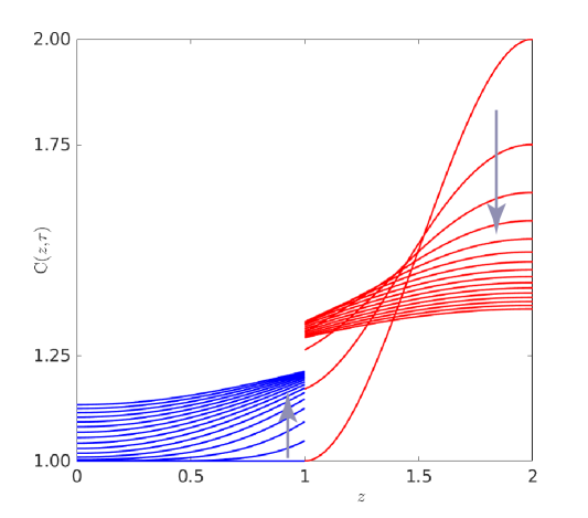
(b)  

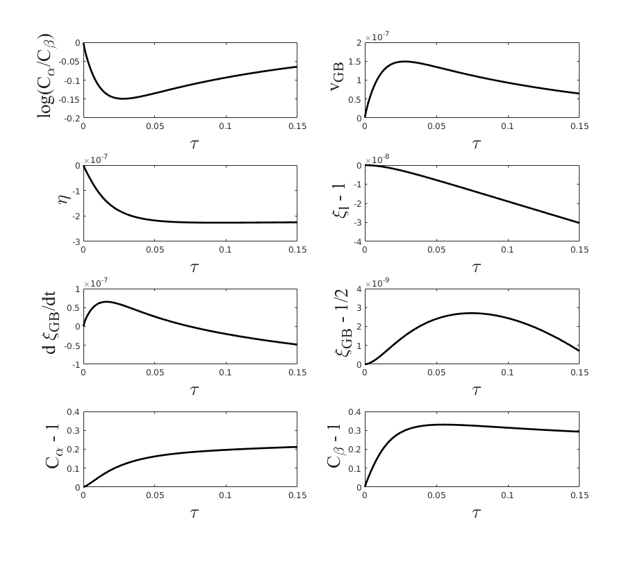
Figure 7: Vacancy concentration profiles (a) and various interfacial quantities. (b) obtained by numerical solution of the model. The concentration profiles are shown at times $\tau$ ranging from 0 to 1.5 at 0.1 increments. The arrow indicates the direction of time. The model parameters correspond to case 8 in Table 2.

In the second example, all three parameters $\lambda$, $\lambda_{t}$ and $\rho$ are small (case 8 in Table 2). The difference from the previous example is that the GB is now a strong diffusive barrier to the vacancies. To the first approximation, the grains can be treated as isolated from each other. Then the vacancy concentration in grain $\alpha$ should remain $C_{\alpha}\equiv 1$ while in grain $\beta$ it should tend to even out and eventually becomes uniform at $C_{\beta}=1.5$. This process should create a vacancy concentration gap $\Delta C=C_{\beta}-C_{\alpha}=0.5$ at the boundary. The numerical solution shows that a large gap does initially arise. However, the vacancies soon begin to leak into grain $\alpha$, reducing the gap and, in the long run, closing it (Fig. 7). The vacancy concentration tends to level at the conservation-dictated value of 1.25. A notable feature of this process is that the gap creates a driving force for GB migration, as evident from the equation

$$\eta_{GB}=-\lambda\ln\dfrac{C_{\alpha}}{C_{\beta}}$$ (71)

obtained by combining Eqs.(46) and (52). Although the mobility $\lambda$ is small, the GB still moves with a velocity $\eta_{GB}$ that is orders of magnitude higher than in the previous example where the gap was small. This example demonstrates the physical phenomenon of vacancy-driven GB migration.

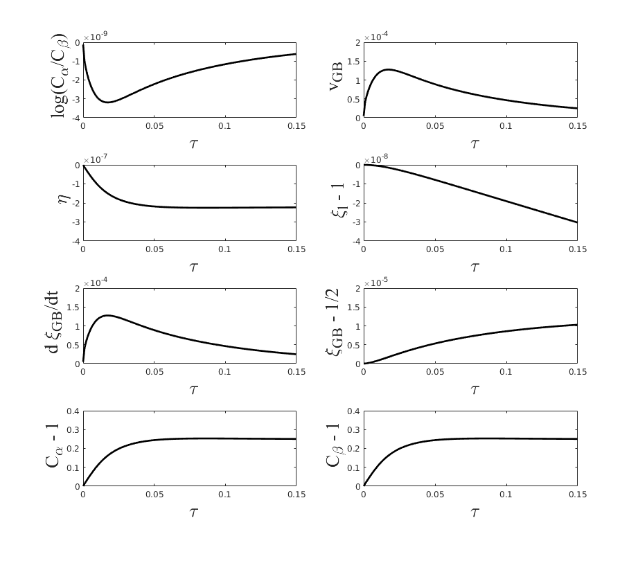
Figure 8: Vacancy concentration profiles (a) and various interfacial quantities. (b) obtained by numerical solution of the model. The concentration profiles are shown at times $\tau$ ranging from 0 to 1.5 at 0.1 increments. The arrows indicate the direction of time. The model parameters correspond to case 7 in Table 2.

In the third example, corresponding to case 7 in Table 2, the vacancy-driven GB migration occurs much faster than in the previous example. We keep the same small values of $\lambda_{t}$ and $\rho$ (slow diffusion across the GB and negligible vacancy absorption), but the GB mobility $\lambda$ is now high. Interestingly, the concentration gap at the GB becomes much smaller (Fig. 8). Nevertheless, due to the high GB mobility this small gap is still capable of driving the boundary motion into grain $\beta$ with a much higher velocity than in the previous examples.

It should be noted that the relation between the vacancy concentration gap and the GB motion is rather convoluted. While the GB motion is driven by the gap, it also strongly reduces the gap. To understand the underlying mechanism, suppose a large gap initially exists due to the diffusion barrier at the GB. Driven by this gap, the boundary moves into the grain in which the vacancy concentration is smaller (cf. Eq.(71)). The gap is then left behind, inside the advancing grain, and can now smooth out by lattice diffusion. In the new position, the GB starts creating a new concentration gap by acting as a diffusion barrier, until the gap becomes large enough to move the boundary into a new position, leaving the gap behind for smoothing by lattice diffusion. In reality the process is continuous rather than incremental, but the mechanism is the same. The process eventually reaches a kinetic balance between the gap-driven GB motion and the motion-induced gap suppression. The remarkable result of this gap-motion coupling is that, in spite of the existence of the strong diffusion barrier at the GB, the vacancy composition profiles look very similar to those in the first example (cf. Fig. 6), in which the boundary did not impose any diffusion barrier but was immobile. This similarity confirms the prominent role of the parameter combination $2\lambda+\lambda_{t}$ in this model, as suggested by the normal mode analysis. In the two cases compared here, this combination is large but for very different reasons: $2\lambda\ll\lambda_{t}$ in one case and $2\lambda\gg\lambda_{t}$ in the other. Note also that the profiles gradually develop a shape that is nearly odd with respect to the GB position, which is a feature the $\kappa_{\lambda}$ normal mode. Thus, the gap-motion coupling provides the mechanistic explanation of why $\lambda$ and $\lambda_{t}$ control the vacancy relaxation process predominantly in this combination and not separately.

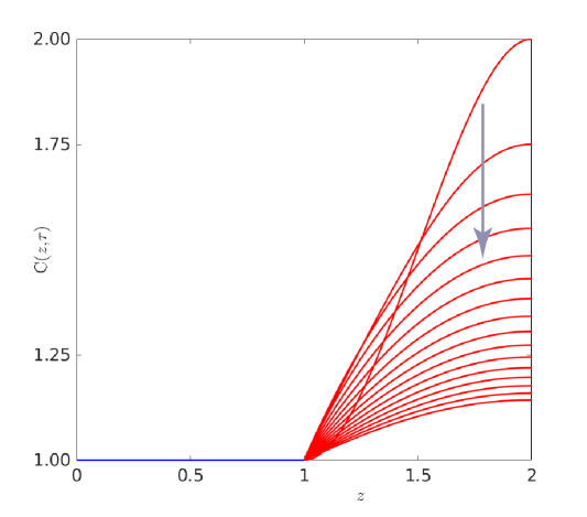
(b)  

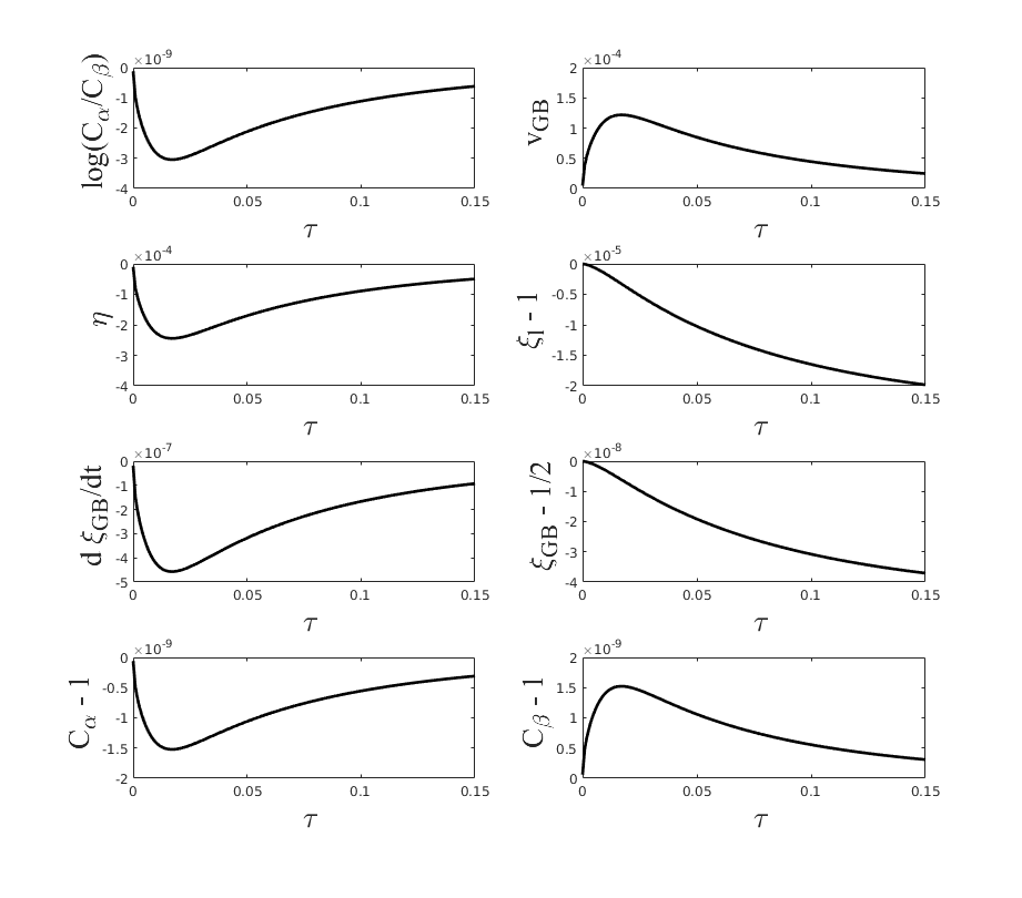
Figure 9: Vacancy concentration profiles (a) and various interfacial quantities. (b) obtained by numerical solution of the model. The concentration profiles are shown at times $\tau$ ranging from 0 to 1.5 at 0.1 increments. The arrow indicates the direction of time. The model parameters correspond to case 1 in Table 2.

Finally, example four features the effect of vacancy absorption at the boundary. The model parameters correspond to case 1 in Table 2, in which the vacancy diffusion across the boundary is fast (large $\lambda_{t}$), the GB is highly mobile (large $\lambda$), and it acts as a powerful sink/source of vacancies (large $\rho$). The GB maintains a nearly perfect equilibrium concentration at all times (Fig. 9). This is a standard assumption in most models describing GBs as vacancy sinks. The vacancies diffusing toward the boundary from grain $\beta$ are eliminated at the boundary and do not penetrate into grain $\alpha$. As a result, grain $\beta$ shrinks while grain $\alpha$ remains intact in both its size and the vacancy concentration. Since the lattice velocity $\eta$ is negative and much larger in magnitude than $d\xi_{GB}/d\tau$, the process can be described as GB migration into grain $\beta$ with the velocity $\eta_{GB}=-\eta/2$ driven by the small but non-negligible vacancy concentration jump.

IV Conclusions

We have applied a sharp-interface model to study the interactions of a planar GB with non-equilibrium vacancies in the presence of mechanical stresses. By contrast to most of the existing models, the present model includes the vacancy generation and absorption processes (or equivalently, lattice site generation/absorption) by the GB. The model predicts a set of coupled kinetic processes that can occur at the GB, including vacancy diffusion toward or away from the boundary, vacancy diffusion across the GB, the GB migration process, and the vacancy generation/absorption at the GB. The rates of these processes are linked to the respective thermodynamic forces, which were previously (Mishin et al., 2015) identified from the equation for the total free energy rate of decrease.

Analysis of the model and the numerical calculations reported here reveal a number of effects arising due to the coupling among the different processes. In particular, the GB motion accelerates the absorption of over-saturated vacancies and/or generation of new vacancies into the grains if their concentration is below equilibrium. If the vacancy concentration is different on either side of the GB, a driving force arises causing GB motion into the grain with the larger concentration. At the same time, the GB motion reduces the concentration jump across the GB and thus the driving force for its migration. The vacancy concentration jump is also influenced by the vacancy generation/absorption process. The different vacancy concentrations result in different driving forces for the vacancy generation or absorption, and thus different generation/absorption rates. The difference in the generation/absorption rates on either side of the GB causes its migration into the grain with faster absorption or slower generation. All these processes are influenced by the rate of vacancy diffusion across the GB. Slow cross-boundary diffusion creates a vacancy concentration jump, which creates a driving force for the GB motion, which in turn affects the rate of vacancy generation and absorption.

Given this coupling among the kinetic processes involved, any meaningful model of vacancy-GB interactions must include all of these processes, describing them by a set of coupled equations. The model presented here achieves this goal and identifies the key combinations of the material parameters that can be utilized to control the vacancy-GB interaction process for various applications. Potential applications of the model include radiation damage healing, diffusional creep, irradiation creep, and solid-state sintering (Herring, 1951, 1953; Kazaryan et al., 1999; Wang, 2006; Li et al., 2011; Abdeljawad et al., 2019).

The present version of the model is based on many simplifying assumptions and approximations, some of which can be lifted in the future. For example, the model can be generalized to multi-component solid solutions containing both vacancies and interstitials. This should allow one to describe the formation of segregation atmospheres and denuded zones near GBs. Although the GB studied here was planar, extension to curved GBs is also possible along the lines discussed in (Mishin et al., 2015). it should also be noted that some of the kinetic parameters of the model can be obtained by atomistic calculations, including the lattice and grain boundary diffusion coefficients as well as the grain boundary mobility. Obtaining this information from atomistic studies of crystallographically specific grain boundaries, and using the present model, could provide a better understanding of the effect of bicrystallography and atomic structure of grain boundaries on their capacity to absorb or generate point defects.

Acknowledgement: Y.M was supported by the National Institute of Standards and Technology, Material Measurement Laboratory, the Materials Science and Engineering Division.

Appendix A: Table of notation

Table 1: List of notation in the order of appearance in the paper. Indices $\alpha$ and $\beta$ label the two grains separated by a grain boundary.

Notation		Meaning
$\mathbf{v}_{L}^{\alpha}$ and $\mathbf{v}_{L}^{\beta}$		Lattice velocities in the grains with respect to laboratory reference frame.
$\mathbf{J}_{L}^{\alpha}$ and $\mathbf{J}_{L}^{\beta}$		Atomic diffusion fluxes in the grains with respect to the lattice reference frames.
$\mathbf{J}_{b}$		2D atomic diffusion flux in grain boundary.
$\mathbf{J}_{n}$		Atomic diffusion flux across grain boundary.
$\mathbf{n}^{\alpha}$		Normal to grain boundary pointing from grain $\alpha$ into grain $\beta$.
$\mathbf{\boldsymbol{\sigma}_{\alpha}}$ and $\mathbf{\boldsymbol{\sigma}_{\beta}}$		Stress tensors in the grains.
$\omega_{\alpha}$ and $\omega_{\beta}$		Grand-canonical potentials per unit volume in the grains.
$f_{s}^{\alpha}$ and $f_{s}^{\beta}$		Free energies per lattice site in the grains.
$\Omega_{\alpha}$ and $\Omega_{\beta}$		Atomic volumes per lattice site in the grains.
$M_{\alpha}$ and $M_{\beta}$		Diffusion potentials of atoms relative to the vacancies in the grains.
$c_{\alpha}$ and $c_{\beta}$		Atomic concentrations (fractions of occupied lattice sites) in the grains.
$L_{\alpha}$ and $L_{\beta}$		Diffusion kinetic coefficients in the grains.
$\mathbf{x},t$		Position and time.
$\mathbf{A}_{\alpha}$ and $\mathbf{A}_{\beta}$		General vector fields in the grains extrapolated to the grain boundary.
$\left[\mathbf{A}\right]\equiv\mathbf{A}_{\alpha}-\mathbf{A}_{\beta}$		Jump of the vector fields across the grain boundary.
$\left\langle\mathbf{A}\right\rangle\equiv(\mathbf{A}_{\alpha}+\mathbf{A}_{\beta})/2$		Average value of the vector fields across the grain boundary.
$L_{t}$ and $L_{p}$		Kinetic coefficients for trans-boundary and intra-boundary diffusion.
$\nu_{\alpha}$ and $\nu_{\beta}$		Numbers of atoms added to the grains per unit area and unit time.
$\nabla_{b}$		2D gradient in grain boundary plane.
$\mathbf{v}_{b}$		Grain boundary velocity relative to laboratory reference frame.
$\mathbf{s}$		Grain boundary traction vector.
$\bot$ and $\|$		Subscripts for normal and tangential components.
$R$		Kinetic coefficient for vacancy creation and annihilation in the grain boundary.
$L_{GB}$		Kinetic coefficient for grain boundary mobility.
$\beta$		Shear coupling factor.
$v_{GB}$		Grain boundary velocity with respect to the mean lattice velocity of the grains.
$\mathbf{t}$		Direction of shear-coupled grain boundary motion.
$K_{s}$		Kinetic coefficient for grain boundary sliding.
$\Delta\Omega_{v}$		Vacancy relaxation volume.
$\boldsymbol{\varepsilon}^{0}$		Stress-free strain due to vacancies.
$\Omega^{\prime}$		Atomic volume in the reference state of strain.
$\mathbf{S}$		Tensor of elastic compliances.
$\sigma_{h}$		Hydrostatic part of the stress tensor.
$M^{*}$		Equilibrium diffusion potential.
$c^{*}$		Equilibrium atomic concentration in stress-free grains.
$kT$		Thermal energy ($T$ temperature, $k$ Boltzmann’s constant).
$c_{v}$		Vacancy concentration (fraction of vacant lattice sites).
$c_{v}^{*}$		Equilibrium vacancy concentration.
$D$		Atomic diffusion coefficient.
$x_{GB}$		Grain boundary position.
$l(t)$		Bicrystal length as a function of time.
$l_{0}$		Initial bicrystal length.
$E$, $\nu$		Young modulus and Poisson’s ratio of the material.
$L_{t}^{\prime}$		Scaled kinetic coefficient of trans-boundary diffusion.
$\tau$		Dimensionless time.
$\xi$		Dimensionless coordinate.
$\xi_{l}$		Dimensionless bicrystal length.
$\xi_{GB}$		Dimensionless grain boundary position.
$\eta$		Dimensionless lattice velocity.
$s$		Dimensionless stress.
$\lambda_{t}$		Dimensionless kinetic coefficient of trans-boundary diffusion.
$\lambda$		Dimensionless grain boundary mobility.
$\rho$		Dimensionless kinetic coefficient for vacancy creation and annihilation in the grain boundary.
$b$		Dimensionless vacancy relaxation volume.
$\hat{C}$		Dimensionless amplitude of the excess of the vacancy concentration.
$\kappa$, $\kappa_{\rho}$, $\kappa_{\lambda}$		Relaxation wave numbers in the linear stability analysis.
$Z_{\rho}$, $Z_{\lambda}$		Dimensionless parameters governing the relaxation modes in the linear stability analysis.

Appendix B: Linear stability analysis

The governing equations (47)-(52) with $s=0$ can be linearized around the equilibrium state with $C_{\alpha}=C_{\beta}=1$, $\xi_{GB}=1/2$, $\eta=0$ and $\xi_{l}=1$. The linearized equations for the perturbed vacancy concentrations $c_{a}(\xi,\tau)$ and $c_{b}(\xi,\tau)$ are

$$\dfrac{\partial c_{a}}{\partial\tau}=\dfrac{\partial^{2}c_{a}}{\partial\xi^{2}},\>\>\>\mathrm{0\leq\xi\leq 1/2},$$ (72)

$$\dfrac{\partial c_{b}}{\partial\tau}=\dfrac{\partial^{2}c_{b}}{\partial\xi^{2}},\>\>\>\mathrm{1/2\leq\xi\leq 1,}$$ (73)

with the boundary conditions

$$\dfrac{\partial c_{a}}{\partial\xi}(0,\tau)=0,\>\>\>\dfrac{\partial c_{b}}{\partial\xi}(1,\tau)=0,$$

The linearized boundary conditions at the GB ($\xi=1/2$) are

$$-2\dfrac{d\xi_{GB}}{d\tau}+\eta+c_{v}^{*}\left(\dfrac{\partial c_{a}}{\partial\xi}+\dfrac{\partial c_{b}}{\partial\xi}\right)=-\lambda_{t}\left(c_{a}-c_{b}\right),$$ (74)

$$\eta+c_{v}^{*}\left(\dfrac{\partial c_{a}}{\partial\xi}-\dfrac{\partial c_{b}}{\partial\xi}\right)=0,$$ (75)

$$\eta=-\rho\dfrac{c_{a}+c_{b}}{2},$$ (76)

$$\dfrac{d\xi_{GB}}{d\tau}=\dfrac{1}{2}\eta-\lambda\left(c_{a}-c_{b}\right).$$ (77)

We seek a normal mode solution of the linearized equations in the form

$$c_{a}(\xi,\tau)=C_{a}(\xi)\exp(-\kappa^{2}\tau),\>\>\>c_{b}(\xi,\tau)=C_{b}(\xi)\exp(-\kappa^{2}\tau),$$

$$\xi_{GB}(\tau)=\dfrac{1}{2}+X_{GB}\exp(-\kappa^{2}\tau),\>\>\>\eta(\tau)=V\exp(-\kappa^{2}\tau),$$

where we anticipate damped solutions with a real, positive decay rate $\kappa^{2}>0$. The diffusion equations become

$$-\kappa^{2}C_{a}=\dfrac{\partial^{2}C_{a}}{\partial\xi^{2}},\>\>\>\mathrm{0\leq\xi\leq 1/2},$$ (78)

$$-\kappa^{2}C_{b}=\dfrac{\partial^{2}C_{b}}{\partial\xi^{2}},\>\>\>\mathrm{1/2\leq\xi\leq 1,}$$ (79)

with the boundary conditions

$$\dfrac{dC_{a}}{d\xi}(0)=0,\>\>\>\dfrac{dC_{b}}{d\xi}(1)=0.$$

The solutions are

$$C_{a}(\xi)=F\cos\xi\kappa,\>\>\>C_{b}(\xi)=G\cos\kappa(\xi-1),$$

where $F$ and $G$ are constants. Inserting them back in Eqs.(74)-(77), the boundary conditions at $\xi=1/2$ become

$$2\kappa^{2}X_{GB}+V-c_{v}^{*}\kappa\sin(\kappa/2)(F-G)+\lambda_{t}\cos(\kappa/2)(F-G)=0,$$

$$V+c_{v}^{*}\kappa\sin(\kappa/2)(F+G)=0,$$

$$2V+\rho\cos(\kappa/2)(F+G)=0,$$

$$2\kappa^{2}X_{GB}+V-2\lambda\cos(\kappa/2)(F-G)=0.$$

Treating $X_{GB}$, $V$, $(F+G)$ and $(F-G)$ as unknowns, we have a homogeneous linear system of equations

$$\begin{bmatrix}2\kappa^{2}&&1&&0&&&\lambda_{t}\cos(\kappa/2)-c_{v}^{*}\kappa\sin(\kappa/2)\\ 0&&1&&c_{v}^{*}\kappa\sin(\kappa/2)&&&0\\ 0&&2&&\rho\cos(\kappa/2)&&&0\\ 2\kappa^{2}&&1&&0&&&-2\lambda\cos(\kappa/2)\end{bmatrix}\begin{bmatrix}X_{GB}\\ V\\ F+G\\ F-G\end{bmatrix}=\begin{bmatrix}0\\ 0\\ 0\\ 0\end{bmatrix}.$$ (80)

This system of equations has nontrivial solutions if its determinant is zero. This condition gives the dispersion relation

$$2\kappa^{2}\left(\rho\cos(\kappa/2)-2c_{v}^{*}\kappa\sin(\kappa/2)\right)\left((2\lambda+\lambda_{t})\cos(\kappa/2)-c_{v}^{*}\kappa\sin(\kappa/2)\right)=0,$$ (81)

which factors into three branches that will be referred to as the $\kappa=0$ branch, the $\kappa_{\rho}$ branch, and the $\kappa_{\lambda}$ branch.

On the $\kappa=0$ branch, the linear system (80) becomes

$$\begin{bmatrix}0&1&0&\lambda_{t}\\ 0&1&0&0\\ 0&2&\rho&0\\ 0&1&0&-2\lambda\end{bmatrix}\begin{bmatrix}X_{GB}\\ V\\ F+G\\ F-G\end{bmatrix}=\begin{bmatrix}0\\ 0\\ 0\\ 0\end{bmatrix}.$$ (82)

and has the trivial solution $F=G=V=0$ with arbitrary $X_{GB}$. This branch reflects the fact that the equilibrium can be reached for any GB position $X_{GB}$.

On the $\kappa_{\rho}$ branch, the root $\kappa_{\rho}$ of Eq.(81) satisfies the condition

$$\dfrac{\rho}{2c_{v}^{*}\kappa_{\rho}}=\tan\dfrac{\kappa_{\rho}}{2},$$

which is a transcendental equation of the form

$$\dfrac{Z}{x}=\tan x$$ (83)

with a constant $Z$. It has a well-known graphical interpretation with the root given by the intersection of the left-hand side $y=Z/x$ and the right hand side $y=\tan x$. For positive $Z$, the smallest root lies in the range $0<x<\pi/2$. On this branch, the parameter $Z$ is

$$Z_{\rho}=\dfrac{\rho}{4c_{v}^{*}}.$$ (84)

The linear system (80) takes the form

$$\begin{bmatrix}2\kappa_{\rho}^{2}&&1&&0&&(\lambda_{t}-\rho/2)\cos(\kappa_{\rho}/2)\\ 0&&2&&\rho\cos(\kappa_{\rho}/2)&&0\\ 0&&2&&\rho\cos(\kappa_{\rho}/2)&&0\\ 2\kappa_{\rho}^{2}&&1&&0&&-2\lambda\cos(\kappa_{\rho}/2)\end{bmatrix}\begin{bmatrix}X_{GB}\\ V\\ F+G\\ F-G\end{bmatrix}=\begin{bmatrix}0\\ 0\\ 0\\ 0\end{bmatrix}$$ (85)

and the corresponding normal mode is proportional to

$$\begin{bmatrix}X_{GB}\\ V\\ F+G\\ F-G\end{bmatrix}=\begin{bmatrix}\rho\cos(\kappa_{\rho}/2)\\ -2\rho\kappa_{\rho}^{2}\cos(\kappa_{\rho}/2)\\ 4\kappa_{\rho}^{2}\\ 0\end{bmatrix}.$$ (86)

Since $F=G$, the vacancy concentration is continuous across the GB. Note that in this mode, the GB migration velocity $d\xi_{GB}/d\tau-\eta/2=0$. The boundary does not move relative to the mean velocity of the grains. The only GB process occurring is the vacancy generation and absorption.

On the $\kappa_{\lambda}$ branch, the root $\kappa_{\lambda}$ of Eq.(81) satisfies the condition

$$\dfrac{2\lambda+\lambda_{t}}{c_{v}^{*}\kappa_{\lambda}}=\tan\dfrac{\kappa_{\lambda}}{2},$$

which is the same transcendent equation (83) with the constant

$$Z_{\lambda}=\dfrac{2\lambda+\lambda_{t}}{2c_{v}^{*}}.$$ (87)

The linear system becomes

$$\begin{bmatrix}2\kappa_{\lambda}^{2}&&1&&0&&&-2\lambda\cos(\kappa_{\lambda}/2)\\ 0&&1&&(2\lambda+\lambda_{t})\cos(\kappa_{\lambda}/2)&&&0\\ 0&&2&&\rho\cos(\kappa_{\lambda}/2)&&&0\\ 2\kappa_{\lambda}^{2}&&1&&0&&&-2\lambda\cos(\kappa_{\lambda}/2)\end{bmatrix}\begin{bmatrix}X_{GB}\\ V\\ F+G\\ F-G\end{bmatrix}=\begin{bmatrix}0\\ 0\\ 0\\ 0\end{bmatrix}$$ (88)

and the normal mode is proportional to

$$\begin{bmatrix}X_{GB}\\ V\\ F+G\\ F-G\end{bmatrix}=\begin{bmatrix}\lambda\cos(\kappa_{\lambda}/2)\\ 0\\ 0\\ \kappa_{\lambda}^{2}\end{bmatrix}.$$ (89)

In this mode, there is no driving force for the vacancy creation or absorption at the GB and thus no lattice flow ($V=0$). The boundary can migrate and the vacancy concentration profile is discontinuous at the boundary, while its spatial derivative remains continuous ($F=-G$).

Table 2: Summary of model parameters for the numerical study of mixed-mode vacancy relaxation.

Case		$\lambda_{t}$		$\lambda$		$\rho$		$Z_{\rho}$		$Z_{\lambda}$		GB properties
1		$300$		$4\times 10^{4}$		$10^{10}$		$5.0\times 10^{13}$		$8.03\times 10^{8}$		Mobile, efficient vacancy sink/source, weak diffusion barrier.
2		$300$		$10^{-6}$		$10^{10}$		$5.0\times 10^{13}$		$3.0\times 10^{6}$		Sluggish, efficient vacancy sink/source, weak diffusion barrier.
3		$300$		$4\times 10^{4}$		$10^{-6}$		$5.0\times 10^{-3}$		$8.03\times 10^{8}$		Mobile, poor vacancy sink/source, weak diffusion barrier.
4		$300$		$10^{-6}$		$10^{-6}$		$5.0\times 10^{-3}$		$3.0\times 10^{6}$		Sluggish, poor vacancy sink/source, weak diffusion barrier.
5		$10^{-3}$		$4\times 10^{4}$		$10^{10}$		$5.0\times 10^{13}$		$8.03\times 10^{8}$		Mobile, efficient vacancy sink/source, strong diffusion barrier.
6		$10^{-3}$		$10^{-6}$		$10^{10}$		$5.0\times 10^{13}$		$10.02$		Sluggish, efficient vacancy sink/source, strong diffusion barrier.
7		$10^{-3}$		$4\times 10^{4}$		$10^{-6}$		$5.0\times 10^{-3}$		$8.0\times 10^{8}$		Mobile, poor vacancy sink/source, strong diffusion barrier.
8		$10^{-3}$		$10^{-6}$		$10^{-6}$		$5.0\times 10^{-3}$		$10.02$		Sluggish, poor vacancy sink/source, strong diffusion barrier.

(a)  

(a)  

(b)  

(a)  

(a)  

(a)  

(a)  

(b)  

(a)

References

- Nabarro (1948) F. R. Nabarro, Deformation of crystals by the motion of single ions, in: Report of a Conference on Strength of Solids, The Physical Society, London, UK, 1948, pp. 75–90.
- Herring (1950) C. J. Herring, Diffusional viscosity of polycrystalline solids, J. Appl. Phys. 21 (1950) 437–445.
- Coble (1963) R. L. Coble, A model for boundary diffusion controlled creep in polycrystalline materials, J. Appl. Phys. 34 (1963) 1679–1682.
- Mohamed and Li (2001) F. A. Mohamed, Y. Li, Creep and superplasticity in nanocrystalline materials: current understanding and future prospects, Mater. Sci. Eng. A 298 (2001) 1–15.
- Svoboda et al. (2006) J. Svoboda, F. D. Fischer, P. Fratzl, Diffusion and creep in multi-component alloys with non-ideal sources and sinks for vacancies, Acta Mater. 54 (2006) 3043–3053.
- Svoboda and Fischer (2011) J. Svoboda, F. D. Fischer, Modelling of the influence of the vacancy source and sink activity and the stress state on diffusion in crystalline solids, Acta Mater. 59 (2011) 1212–1219.
- Mishin et al. (2013) Y. Mishin, J. A. Warren, R. F. Sekerka, W. J. Boettinger, Irreversible thermodynamics of creep in crystalline solids, Phys. Rev. B 88 (2013) 184303.
- Herring (1951) C. Herring, Surface tension as a motivation for sintering, in: The Physics of Powder Metallurgy, McGraw-Hill, New York, 1951, pp. 143–179.
- Herring (1953) C. Herring, The use of classical macroscopic concepts in surface-energy problems, in: R. Gomer, C. S. Smith (Eds.), Structure and Properties of Solid Surfaces, The Univ. of Chicago Press, Chicago, Illinois, 1953, pp. 5–81.
- Mishin et al. (2015) Y. Mishin, G. B. McFadden, R. F. Sekerka, W. J. Boettinger, Sharp interface model of creep deformation in crystalline solids, Phys. Rev. B 92 (2015) 064113.
- Kazaryan et al. (1999) A. Kazaryan, Y. Wang, B. R. Patton, Generalized phase field approach for computer simulation of sintering: Incorporation of rigid-body motion, Scripta Mater. 41 (1999) 487–492.
- Wang (2006) Y. U. Wang, Computer modeling and simulation of solid-state sintering: A phase field approach, Acta Mater. 54 (2006) 953–961.
- Abdeljawad et al. (2019) F. Abdeljawad, D. S. Bolintineanu, A. Cook, H. Brown-Shaklee, C. DiAntonio, D. Kammler, R. Roach, Sintering processes in direct ink additive manufacturing: A mesoscopic modeling approach, Acta Mater. 169 (2019) 60–75.
- Li et al. (2011) J. Li, S. Sarkar, W. T. Cox, T. J. Lenosky, E. Bitzek, Y. Wang, Diffusive molecular dynamics and its application to nanoindentation and sintering, Phys. Rev. B 84 (2011) 054103.
- Sup (????) See the online supplementary material to this article at https://doi.org/10.1016/j.actamat.2019.11.044
- Cahn et al. (2006a) J. W. Cahn, Y. Mishin, A. Suzuki, Duality of dislocation content of grain boundaries, Philos. Mag. 86 (2006a) 3965–3980.
- Cahn et al. (2006b) J. W. Cahn, Y. Mishin, A. Suzuki, Coupling grain boundary motion to shear deformation, Acta Mater. 54 (2006b) 4953–4975.
- Sutton and Balluffi (1995) A. P. Sutton, R. W. Balluffi, Interfaces in Crystalline Materials, Clarendon Press, Oxford, 1995.
- Gu et al. (2017) Y. Gu, J. Han, S. Dai, Y. Zhu, Y. Xiang, D. J. Srolovitz, Point defect sink efficiency of low-angle tilt grain boundaries, J. Mech. Phys. Solids 101 (2017) 166–179.
- Han et al. (2018) J. Han, S. L. Thomas, D. J. Srolovitz, Grain-boundary kinetics: A unified approach, Prog. Mater. Sci. 98 (2018) 386–476.
- Borovikov et al. (2013) V. Borovikov, X. Z. Tang, D. Perez, X. M. Bai, B. P. Uberuaga, A. F. Voter, Influence of point defects on grain boundary mobility in bcc tungsten, J. Phys.: Condens. Matter 25 (2013) 035402.
- Herring (1949) C. Herring, in: R. Gomer, C. S. Smith (Eds.), The Physics of Powder Metallurgy, McGraw-Hill, New York, 1949.
- Kraftmakher (1998) Y. Kraftmakher, Equilibrium vacancies and thermophysical properties of metals, Physics Reports 299 (1998) 79–188.
- Was (2017) G. S. Was, Irradiation creep and growth, in: Fundamentals of Radiation Materials Science, Springer, New York, NY, 2017, pp. 735–791.