Comparison of The UV and Optical Fe II Emission in Type 1 AGNs

Abstract

We present the kinematical properties of the UV and optical Fe II emission gas based on the velocity shift and line width measurements of a sample of 223 Type 1 active galactic nuclei (AGNs) at 0.4 $<$ z $<$ 0.8. We find a strong correlation between the line widths of the UV and optical Fe II emission lines, indicating that both Fe II emission features arise from similar distances in the broad line region (BLR). However, in detail we find differing trends, depending on the width of Fe II. While the velocity shifts and dispersions of the UV Fe II (Fe II_uv) and optical Fe II (Fe II_opt) emission lines are comparable to each other for AGNs with relatively narrow Fe II_opt line widths (i.e., FWHM ¡ 3200 km s^-1; Group A), Fe II_opt is broader than Fe II_uv for AGNs with relatively broad Fe II_opt  (i.e., FWHM ¿ 3200 km s^-1; Group B). Fe II emission lines are on average narrower than H$\beta$ and Mg II for Group A, indicating the Fe II emission region is further out in the BLR, while for Group B AGNs Fe II_opt is comparable to H$\beta$ and broader than Mg II. While Fe II emission lines are on average redshifted ($40\pm 141$ km s^-1 and $182\pm 95$, respectively for Fe II_uv and Fe II_opt), indicating inflow, the sample as a whole shows a large range of velocity shifts, suggesting complex nature of gas kinematics.

1. INTRODUCTION

Active galactic nuclei (AGNs) present diverse components of broad and narrow emission lines in the UV to optical spectral range. These spectral properties reflects the geometric structure, distribution of emissivity, and kinematics of the gas. The Fe II emission blends are often strongly detected around the UV Mg II 2798Å and the optical H$\beta$ 4861Å lines. Since 1960s, a number of studies has investigated the properties of Fe II emission (e.g., Greenstein & Schmidt, 1964; Kwan & Krolik, 1981; Joly, 1987; Wampler & Oke, 1967). Iron is mainly produced by Type Ia supernovae (SNe) in a binary system, and by Type II SNe in massive stars along with heavy $\alpha$ elements, e.g., O, Ne, and Mg. Because of their different time scales of formation, the Fe II/Mg II line flux ratio is often used to investigate chemical evolution as the first order-proxy for the Fe/Mg element ratio (e.g, De Rosa et al., 2011; Sameshima et al., 2017; Shin et al., 2019).

The studies of the excitation mechanism and correlation with other emission line properties are important to understanding the origin of Fe II emission, as there are a number of debates on the nature and origin of Fe II in the literature. Fe II emission was considered to originate from the same region as broad emission lines, i.e., H$\beta$. For example, using 87 low-z quasars, for example, Boroson & Green (1992) reported that the line widths of Fe II and H$\beta$ lines were comparable, indicting that they were at similar locations in the broad line region (BLR). In a recent study, however, Popović et al. (2007) reported that the full-width-at-half-maximum (FWHM) of Fe II is $\frac{1}{3}$ of that of the broad H$\beta$ line. Moreover, Hu et al. (2008a) showed that the FWHM of Fe II line is narrower than that of H$\beta$ (i.e., FWHM Fe II $\sim$ $\frac{3}{4}$ FWHM of H$\beta$). These results indicate that Fe II emission may originate from a region that is located further out in the BLR, compared to that emitting the bulk of H$\beta$.

The velocity shift of Fe II emission is also a source of debate. A number of previous studies assumed no systemic velocity shift of Fe II with respect to [O II] (e.g., Boroson & Green, 1992; Kim et al., 2006; Greene & Ho, 2005). However, Hu et al. (2008b) reported that the optical Fe II emission is redshifted by $\sim$400$-$2000 km s^-1 with respect to the peak of the [O III] 5007Å line, using a set of composite spectra, which were constructed with the AGNs at z $<$ 0.8 selected from the Sloan Digital Sky Survey (SDSS). In contrast, Sulentic et al. (2012) disagreed to with Hu et al. (2008b), arguing that the measurement of Fe II velocity shifts is reliable only for AGNs with high signal-to-noise ratio (S/N) spectra. Based on their high S/N composite spectra, Sulentic et al. (2012) claimed no redshift of the optical Fe II emission. Later on, Kovačević-Dojčinović & Popović (2015) reported no significant redshift of the optical Fe II emission using a sample of 293 SDSS AGNs at 0.4 $<$ z $<$ 0.6, while they showed on average a large redshift of the UV Fe II emission with respect to a narrow emission line [OIII] 5007Å (see also Kovačević et al., 2010). For the origin of the difference between Fe II_uv and Fe II_opt, Kovačević-Dojčinović & Popović (2015) suggested the possibility of the asymmetric distribution of the UV-emitting gas clouds in the BLR, as well as the effect of internal shock increasing excitation of UV lines in infalling gas.

There are also issues in the models of the UV and optical Fe II emission, since classical photoionization models cannot explain the measured flux ratio between the optical and UV Fe II emission (e.g., Collin & Joly, 2000; Baldwin et al., 2004; Sameshima et al., 2011). To solve this problem, for example, Baldwin et al. (2004) discussed local micro-turbulence in the emitting gas in their model. Ferland et al. (2009) investigated the role of anisotropy in Fe II emission from local clouds as the anisotropy depends on the column density of individual clouds, potentially causing the difference between optical and UV Fe II emission.

Overall, studying the physical properties of Fe II emission is intriguing. Multiple Fe II emission lines are blended in a typical AGN spectrum, which is composed of the continuum from the central source (accretion disk and reprocessed photons), and host galaxy contribution. Determining accurate Balmer continuum is also difficult since the best-fit result depends on the assumed physical parameters, i.e., electron temperature $\rm T_{e}$, electron density $\rm n_{e}$, optical depths, the shape of the continuum, and the UV Fe II models (e.g., Kovačević et al., 2014 and Kovačević-Dojčinović et al., 2017). Clearly, high S/N spectra and careful spectral decomposition are required to archive reliable measurements of Fe II emission properties.

In this paper, we investigate the kinematical properties of the UV and optical Fe II emission, using a sample of 223 AGNs at 0.4 $<$ z $<$ 0.8. The sample is a composed of 38 moderate-luminosity AGNs with high quality Keck spectra (S/N $\geq$ 10 in 3000Å and $\geq$ 20 in 5100Å) from our previous study (Woo et al., 2018), and 185 AGNs with S/N $\geqslant$ 20 in both 3000 Å and 5100 Å selected from SDSS. The subsamples obtained from SDSS and Keck are complementary to each other, enabling us to explore the physical connections between the UV and optical Fe II emission over a large range of AGN luminosity. Using these AGNs, we investigate Fe II velocity shift, using individual spectra rather than using a composite spectra as previously done by Sulentic et al. (2012) and Hu et al. (2012). One of our main goals is to settle the debate between Hu et al. (2008b) and Sulentic et al. (2012) on the systemic redshift of the optical Fe II emission lines. We present the comparison of the UV and optical Fe II line properties along with the kinematical properties of the broad emission lines, i.e., H$\beta$ and Mg II. Section 2 describes the sample selection, and Section 3 presents the method. The main results are presented in Section 4, followed by Discussion and summary in Section 5 and 6, respectively. The following cosmological parameters are used throughout the paper: $H_{0}=70$ km s^-1 Mpc^-1, $\Omega_{\rm m}=0.30$, and $\Omega_{\Lambda}=0.70$.

2. Sample Selection

We selected a sample of 52 moderate-luminosity AGNs ($\mathrm{\lambda L_{5100}\sim 10^{43.8}-10^{44.4}}$ erg s^-1) at redshift of 0.4 $<$ z $<$ 0.6, which was initially chosen for measuring stellar velocity dispersions of AGN host galaxies to study the evolution of the black hole mass and host spheroid velocity dispersion ($\rm M_{\rm BH}-\sigma_{*}$) relation (Treu et al., 2004; Woo et al., 2006; Woo, 2008; Bennert et al., 2010; Park et al., 2015), and was also presented in a series of papers in the study of the UV and optical M_BH estimators (McGill et al., 2008 and Woo et al., 2018). Observations and data reduction process of the sample can be found in Park et al. (2015); Woo et al. (2018) for the optical and UV spectral ranges. Among 52 targets, we removed 5 AGNs with strong internal extinction (see details in Woo et al., 2018). Among the remaining 47 targets, we selected AGNs based on a couple of criteria: first, S/N $>$ 10 in the continuum at 3000 Å and 20 at 5100 Å. Second, the UV and optical Fe II emissions are strong, i.e., the contribution of the Fe II emission is larger than 20% of the total flux in the UV spectral range of 2600 $-$ 3050 Å, and in the optical spectral range of 4434 $-$ 4684 Å, respectively. As a result, we obtained 38 AGNs with high quality spectra.

We also used the Sloan Digital Sky Survey (SDSS) quasar catalog (Shen et al., 2011) to initially select 14,367 quasars at 0.4 $<$ z $<$ 0.8. The choice of the redshift range is to include both the rest-frame UV and optical Fe II lines. Then, we chose 487 AGNs with high quality spectra (i.e., S/N $\geqslant$ 20) at both 3000 Å and 5100 Å. Among these AGNs, we removed 63 targets, which contain strong absorption lines in the Mg II line profile. In addition, we excluded 10 targets, which have relatively weak [O III] lines and poor fitting results. From the remaining 414 targets, we selected 321 AGNs, which have the contribution of the Fe II emission is greater than 20% in the pseudo continuum as applied to the Keck sample.

After analyzing all emission lines, we further removed the targets with large fractional errors ($\geqslant$ 50%) of the line width and velocity shift of Fe II emission lines (see Section 3.3). The final SDSS sample contained 185 targets with the monochromatic luminosity at 5100Å $\lambda L_{5100}$ ranging from 10^44.5 to 10^46.5 erg s^-1. By combining the SDSS AGNs with the moderate luminosity AGNs from our previous study, we enlarged the luminosity range of the sample for comparing the UV and optical Fe II emission line kinematics.

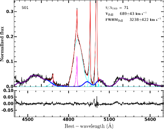
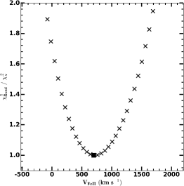
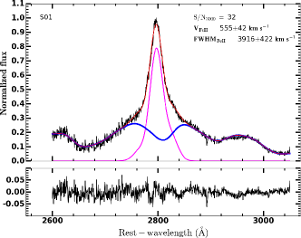
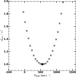
Figure 1.— S01 optical and UV spectra of Keck sample. Top left panel: The rest-frame normalize continuum-subtracted spectra (thick black) and best-fit model (red), adding Fe II emission (blue), broad components (cyan), narrow components (magenta). In the bottom, the residual between the observed spectrum and the combined models is shown (black). Bottom left panel: similarly as color schemes in the top left panel, excepting that magenta shows the best-fit model of Mg II. Top and bottom right panels: $\chi^{2}$ curve as a function of the fixed $\rm V_{FeII}$ of the Fe II template. The best-fit $\rm V_{FeII}$ is shown in solid square.

3. Measurements

We measured the kinematic properties (line width and velocity shift) and fluxes of the UV and optical Fe II emission lines based on the multi-component spectral analysis, following the procedure in our previous studies (Woo et al., 2006; McGill et al., 2008; Park et al., 2015; Woo et al., 2018). In this section, we briefly describe the fitting process for measuring the properties of the UV and optical Fe II emission.

3.1. The UV Spectra Fitting

The fitting process of the UV Fe II  emission lines (Fe II_uv) includes several steps: the observed spectra were fitted simultaneously with a combination of three pseudo-continuum components: a power-law, a Balmer continuum, and a Gaussian-velocity-convolved Fe II template. We used a simple power-law for a continuum from an accretion disk:

$$f_{\lambda}\propto\lambda^{\alpha}$$ (1)

where $\alpha$ is a power-law slope. The Balmer continuum (Grandi, 1982) is calculated as:

$$f_{\lambda}^{BaC}=f_{norm}^{BE}B(\lambda,T_{e})[1-e^{-\tau_{BE}(\frac{\lambda}{\lambda_{BE}})^{3}}]$$ (2)

where $B(\lambda,T_{e})$ is Plank blackbody spectrum at the electron temperature $\rm T_{e}$ of 15,000 K. $\rm\tau_{BE}$ is optical depth at the Balmer edge, $\rm\lambda_{BE}$ = 3646Å. $\rm f_{norm}^{BE}$ is a normalized flux density.

For Fe II emission blends, we adopted the Fe II template based on the I Zw 1 from Tsuzuki et al. (2006). By convolving the Fe II template with a Gaussian function, we generated a series of Fe II models and fitted the observed Fe II with the modes, including a velocity shift as a free parameter. The process was performed in the wavelength range of 2600Å $-$ 3090Å. After subtracting the pseudo-continuum from the observed spectra, we fitted the Mg II line by using a sixth order Gauss-Hermite series (see Section 3.2 in Woo et al., 2018). The best-fit models were determined by $\chi^{2}$ minimization using the nonlinear Levenberg-Marquardt least-squares fitting routine technique, MPFIT (Markwardt, 2009).

3.2. The Optical Spectra Fitting

Similarly, we modeled the optical region with a combination of three components: a single power law, an Fe II template, and a host galaxy template. The fitting was applied in the regions of 4430Å $-$ 4770Å and 5080Å $-$ 5450Å. We used the I Zw 1 Fe II template (Boroson & Green, 1992) and the stellar template from the Indo-US spectral library (Valdes et al., 2004). We convolved the Fe II and host galaxy templates with a Gaussian and determined the velocity shifts and line width of the optical Fe II (Fe II_opt) emission blends as well as those of stellar absorption lines. After subtracting the pseudo-continuum from the observed spectra, we fitted the broad component of the H$\beta$ line by using a sixth order Gauss-Hermite series (see Section 3.1 in Woo et al., 2018). The best-fit models were also archived using the $\chi^{2}$ minimization with the MPFIT.

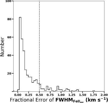
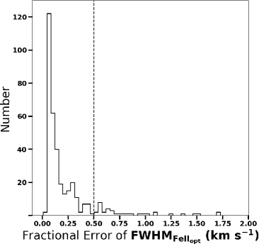
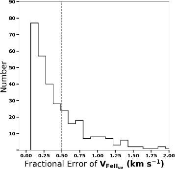
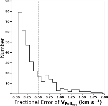
Figure 2.— Fractional error distributions of FWHM and velocity of Fe II_uv and Fe II_opt, respectively. The dash lines show the fraction value of 0.5.

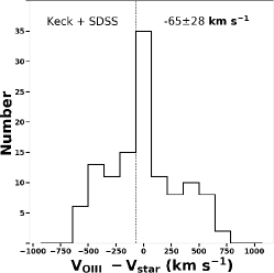
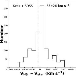
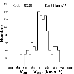
Figure 3.— Distribution of the velocity shift of the peak of [O III] (left panel), the peak of H$\beta$ (middle panel), and the peak of [O II] (right panel), with respect to the systemic velocity measured based on stellar absorption lines, using our Keck and SDSS samples. The dash-line shows the mean of each distribution.

3.3. Fe II Emission Line Widths and Velocity Shifts

The line width and velocity shift of the UV and optical Fe II emission are determined in the fitting process, where we used a series of FeII template with a various width and a velocity shift as free parameters. For the Keck spectra, the measured line widths were corrected for the instrumental resolution of $\sim$145 km s^-1 and $\sim$55 km s^-1 in line dispersion, respectively for the UV and optical spectra, by subtracting the instrumental resolution from the measured velocity in quadrature. We also corrected for the instrumental resolution $R$ $\sim$ 1800 and 2200 of the SDSS spectra. In Figure 1 we present examples of the best-fit result in the UV and optical ranges, which confirms the systemic redshift of Fe II emission lines in both UV and optical. To estimate the confidence of the fit, we used $\chi^{2}$ statistic recipe as described in Section 11.4 of Bevington & Robinson (2003) and Appendix A of Hu et al. (2012). We considered the fit with displacement of fixed $\rm V_{FeII}$ from -500 to 2000 km s^-1.

The measurement errors of line widths and velocity shifts were determined based on the Monte Carlo simulations. We generated 100 mock spectra, for which the flux at each wavelength was randomized by the flux error. Then, we applied the same fitting method for each spectrum. We adopted 1$\sigma$ dispersion of the distribution of the measurements as the error. Figure 2 shows the fractional error of line widths and velocity shifts of Fe II emission lines. To avoid uncertain measurements, we decided to remove the targets with the fractional error of line width or velocity shift larger than 50%.

3.4. Systemic Velocity

To measure the velocity shift of the UV and optical FeII emission blends, we first need to determine the systemic velocity of each target. While the systemic velocity can be best measured based on stellar absorption lines, luminous AGNs typically do not present strong stellar absorption lines. Instead, we consider the peak of the [O III] 5007Å line for determining the systemic velocity as various previous studies have performed (e.g., Hu et al., 2008b; Hu et al., 2012; Sulentic et al., 2012; Kovačević-Dojčinović & Popović, 2015). It is well known that the [O III] line manifests outflows in type 1 and 2 AGNs (e.g., Bae & Woo, 2014; Woo et al., 2016, 2017; Rakshit & Woo, 2018). By using flux weighted center (first moment) of [O III], various previous studies determined the velocity shift of [O III] with respect to stellar absorption lines. However, the peak of [O III] does not show a large velocity shift and can be used as a proxy for stellar absorption lines albeit with large uncertainty. By selecting AGNs, which show a relatively strong stellar component in the continuum ($>$ 30% in the total flux), we tested the difference between the systemic velocity respectively measured based on stellar absorption lines and the peak of [O III] in Figure 3 (left panel). The difference is relatively small with an average of -65 $\pm$ 28 km s^-1, while the worst case shows several hundred km s^-1, suggesting that we may use the peak of the [O III] line for determining systemic velocity since it is close to the stellar velocity.

We also consider the peak of the H$\beta$ line for determining the systemic velocity of each target. Using AGNs with strong stellar absorption lines, we compared the stellar-line-based systemic velocity with the peak of H$\beta$ (Figure 3, middle panel). The difference is an average of -33 $\pm$ 26 km s^-1, which is smaller than the case of the peak of [O III], presumably due to the effect of outflows on the [O III] line profile. Note that careful attention is required in using the peak of H$\beta$ to infer the systemic velocity, since for individual AGNs the peak of H$\beta$ may not be a good tracer of systemic velocity.

In the case of the UV spectra of Keck data, we cannot use H$\beta$ since the UV spectra were obtained independently with a different spectrograph, hence, there could be a systematic shift between UV and optical spectra. Thus, we used the peak of the [O II] 3727Å line to determine the systemic velocity. Figure 3 (right panel) compares the systemic velocity measured from stellar absorption lines and from the peak of [O II]. For most targets, the difference is relatively small with an average of $\sim 41\pm 28$ km s^-1. As in the case of using the H$\beta$ peak, the difference between the peak of [O II] and stellar velocity can be large up to $\pm$750 km s^-1 for individual AGNs. In summary, we used the peak of H$\beta$ for measuring the systemic velocity ($\rm V_{ref}$) in our analysis. In the case of the 38 objects with the Keck UV spectra, we used the peak of [O II] for $\rm V_{ref}$. There are two targets with the Keck spectra, which show large difference in the systemic velocity measured from H$\beta$ and [O II] ($>-500$ km s^-1, SS12 and SS17). We removed these two targets when we compare the velocity shift of Fe II_uv emission lines to other physical quantities.

3.5. Fe II Emission Line fluxes

In addition to the kinematical properties, we also measure the line fluxes based on the Fe II emission lines. Following previous studies in the literature, the line flux of the optical Fe II is integrated over a spectral range of 4434-4684 Å using the best-fit model (see Woo et al., 2015). In the case of the UV Fe II, the line flux is calculated by summing over a spectral range of 2600-3050 Å as similarly done by Kovačević-Dojčinović & Popović (2015).

4. Results

4.1. Comparing UV and Optical Fe II Emission

In this section, we investigate the kinematical properties manifested in the UV and optical Fe II emission lines to understand the connection between two emission line regions.

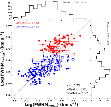
Figure 4.— Comparison of FWHM of Fe II_uv and Fe II_opt. Squares indicate Keck sample with S/N ¿ 20 in the continuum at 3000 Å and 51000 Å . Filled circles show the measurements from SDSS sample. Black dash-lines denote $\rm FWHM_{FeII_{opt}}=FWHM_{FeII_{uv}}$. The correlated coefficient, offset and rms scatter from the black dash line are shown in the plots. Blue samples are $\rm FWHM_{FeII_{opt}}<10^{3.5}$ (Group A), and red samples are $\rm FWHM_{FeII_{opt}}>10^{3.5}$ (Group B).

4.1.1 Line Widths of Fe II Emission Lines

We compare the line width measured from the UV and optical Fe II emission lines in Figure 4. The FWHM of UV Fe II ranges from $\sim$1000 to $\sim$10, 000 km s^-1, with the mean log FWHM (km s^-1) = 3.40 $\pm$ 0.21. In the case of Fe II_opt, the mean log FWHM (km s^-1) is 3.35 $\pm$ 0.23. The comparison shows $\sim$0.2 dex scatter and similar line widths between UV and optical lines. To explore the correlation of the two line widths, we perform the Spearman’s rank-order correlation, finding that Fe II_opt and Fe II_uv lines show are correlated with a correlation coefficient r = 0.73. The results indicate that the UV and optical Fe II emission lines are originated from regions which are closely located to each other as previously reported in the literature (Kovačević-Dojčinović & Popović, 2015).

Nevertheless, we find an interesting trend that the distribution of Fe II_opt FWHM is divided at $\sim$3500 km s^-1. If we separate the sample into two groups: Group A: FWHM of Fe II_opt $<$ $\sim$3200 km s^-1, and Group B: FWHM of Fe II_opt $>$ $\sim$3200 km s^-1, then Group A and Group B show somewhat different comparison. While the line width of Fe II is comparable between UV and optical in Group A, Fe II_opt is broader than Fe II_uv by $\sim$0.1 dex in Group B. Thus, we compare the properties of UV and optical Fe II using these two separate groups in the following sections.

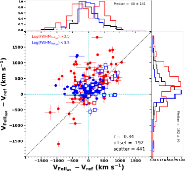
Figure 5.— Comparison of velocity shifts of Fe II_uv and Fe II_opt. Distribution velocity shifts of all sample (black color), Group A (blue color) and Group B (red color) are shown in the histogram panels. Squares indicate Keck sample with S/N ¿ 20 in the continuum at 3000 Å and 5100 Å. Filled circles show the measurements from SDSS sample. Cyan dash-lines show the zero velocity shift. Black dash-lines denote $\rm V_{FeII_{opt}}=V_{FeII_{uv}}$. The correlated coefficient, offset and rms scatter from the black dash line are shown in each panel.

4.1.2 Velocity Shifts of Fe II Emission Lines

We compare the velocity shifts of Fe II_uv and Fe II_opt in Figure 5. For both Fe II_uv and Fe II_opt, the velocity shift ranges around $\pm 1500$ km s^-1, while the mean is 40 $\pm$ 141 km s^-1and 182 $\pm$ 95 km s^-1, respectively for Fe II_uv and Fe II_opt. As described in Section 3.4, we H$\beta$ (and [O II]) shows on velocity shift with respect to stellar absorption lines, with an average of $-33\pm 26$ km s^-1 and $41\pm 28$ km s^-1, respectively. For the uncertainty of the systemic velocity, we added the 3 $\sigma$ uncertainty of the systemic velocity (i.e., a factor of three of the rms dispersion in the distribution of the H$\beta$ or [O II] velocity shift, see Figure 3) to the measurement error determined from the Monte Carlo simulations in quadrature.

The velocity shift correlates between Fe II_uv and Fe II_opt, while the correlation is considerably weaker than the case of the FWHM of Fe II, with r = 0.34. When we examine subsamples, the velocity shifts of Fe II_uv and Fe II_opt in Group A are comparable within the scatter. In the case of Group B, Fe II_opt is on average more redshifted ($\rm V_{FeII_{opt}}$ = 426 $\pm$ 123 km s^-1) than Fe II_uv ($\rm V_{FeII_{UV}}$ = 22 $\pm$ 148 km s^-1).

Overall, there is a large range of velocity shift in both Fe II_uv and Fe II_opt. The majority of AGNs show redshifted Fe II_opt while Fe II_uv is blue-shifted for a significant fraction of AGNs. Note that Fe II_uv and Fe II_opt show a consistent velocity shift, indicating either inflow or outflow motion of gas, with higher velocity of Fe II_opt in general. There are also a small fraction of AGNs, particularly in Group B, that show an opposite sign of the velocity shift between Fe II_uv and Fe II_opt, implying that Fe II_uv gas is outflowing while Fe II_opt gas is inflowing. Note that the measured velocity shift does not entirely depend on the average gas kinematics. The observed emission line reflects the potential anisotropic emission, which may be caused more strongly in UV Fe II from clouds with higher column density (for detailed discussion, see Section 5.2).

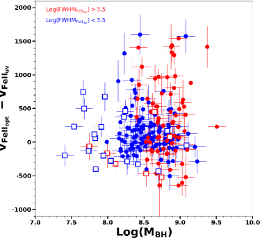
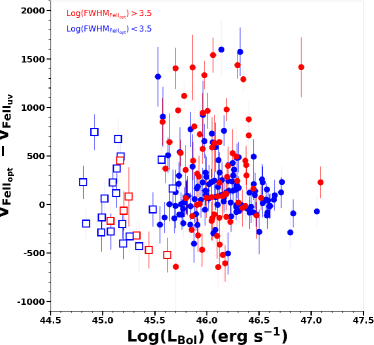
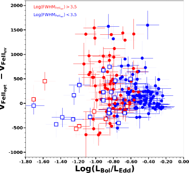
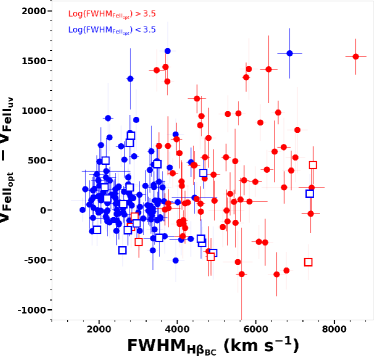
Figure 6.— Comparison of the UV and optical Fe II velocity shift as a function of AGNs properties. Group A ($\rm FWHM_{FeII_{opt}}<10^{3.5}$) is denoted with blue symbols, while Group B ($\rm FWHM_{FeII_{opt}}>10^{3.5}$) is dented with red symbols. Keck and SDSS objects are presented with open and filled symbols, respectively.

4.1.3 Fe II Kinematics vs. AGNs Properties

To explore what is the main driver of the difference in velocity shifts between Fe II_uv and Fe II_opt, we compare them with AGNs properties. In Figure 6, we show the difference in Fe II_uv and Fe II_opt velocity shifts as a function of M_BH, bolometric luminosity, Eddington ratio, and the FWHM of the broad H$\beta$ line. We find no specific trend with M_BH or bolometric luminosity. However, it is interesting to see the difference in the velocity shifts of Group A and B as a function of Eddington ratio luminosity, and FWHM of the H$\beta$ line. Group A sample falls in the group of narrow FWHM H$\beta$ (FWHM $<$ $\sim$4000 km s^-1), and shows relatively small difference in velocity shifts between Fe II_uv and Fe II_opt, while Group B AGNs show larger FWHM H$\beta$ ($>$ $\sim$4000 km s^-1), and display large divergence between Fe II_uv and Fe II_opt velocity shifts. Similarly, the difference in velocity shifts becomes smaller when Eddington ratio is higher ($\rm L_{Bol}/L_{Edd}$ $>$ $\sim$-0.7), while there is a larger discrepancy for lower Eddington ratio AGNs ($\rm L_{Bol}/L_{Edd}$ $<$ $\sim$-0.7).

4.1.4 Fe II vs. Other Emission lines

We compare the line width of Fe II_uv and Fe II_opt with that of the broad emission lines, (i.e., H$\beta$ and Mg II) in Figure 7. First, we investigate the correlation between the line width (FWHM) of Fe II_opt and that of the broad H$\beta$ line. Using the total sample, we determine the correlation coefficient r = 0.85, indicating a good correlation between Fe II_opt and H$\beta$ line widths. We obtain the best-fit slope of 1.15 $\pm$ 0.06, which is close to a linear relationship, while we find a systemic offset of 0.15 dex, indicating that Fe II_opt is an average narrower than H$\beta$ by 30%. For Group A, we find a larger systemic offset of 0.21 dex ($\sim$40%) between Fe II_opt and H$\beta$ in Group A, implying that on average the Fe II_opt emission region is located further out in the BLR, compared to the H$\beta$ emission region. This result is consistent with the result of Hu et al. (2008a), who found that FWHM of Fe II_opt = $\frac{3}{4}$ FWHM of H$\beta$. In contrast, Group B shows comparable line widths between Fe II_opt and H$\beta$, implying that Fe II_opt and H$\beta$ is emitted from the regions, which are close to each other.

Second, we compare Mg II and Fe II_opt, finding similar trends with those of H$\beta$. The widths of Fe II_opt and Mg II are well correlated with r = 0.76. Again, we see the discrepancy between Group A and Group B. For Group A, Fe II_opt is on average narrower than Mg II by 0.15 dex ($\sim$30%), while for Group B, Fe II_opt FWHM is broader than Mg II by 0.1 dex ($\sim$20%).

In the case of UV Fe II, we see no significant difference between Group A and B. The FWHM of Fe II_uv and broad emission lines are well correlated (with r = 0.73, and r = 0.68, respectively for H$\beta$ and Mg II). On average Fe II_uv is narrower than both H$\beta$ (by 0.16 dex) and Mg II (by 0.08 dex), indicating that the Fe II_uv emission line region is further out compared to that of these broad emission lines.

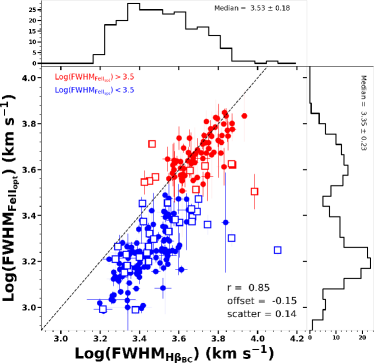
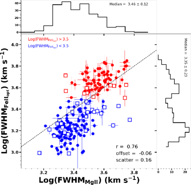
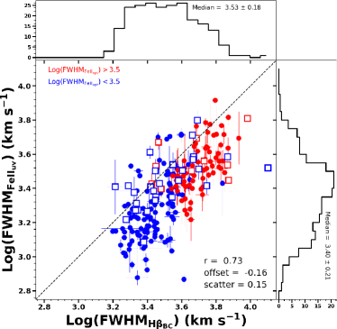
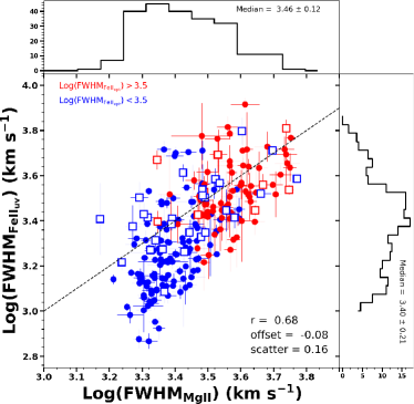
Figure 7.— Comparison of FWHM of Fe II_uv, Fe II_opt with that of Mg II and H$\beta$. Dash-lines denote that FWHM of the quantities of horizon and vertical axes in each panel are same. The correlated coefficient, offset and rms scatter from the black dash line are shown in the plots. Group A ($\rm FWHM_{FeII_{opt}}<10^{3.5}$) is denoted with blue symbols, while Group B ($\rm FWHM_{FeII_{opt}}>10^{3.5}$) is dented with red symbols. Keck and SDSS objects are presented with open and filled symbols, respectively.

4.2. The Fe II_opt to Fe II_uv flux ratio

In this section, we examine the flux ratio between Fe II_opt and Fe II_uv. The Fe II flux is measured in the limited spectral range as described in Section 3.5. We find a large range of the flux ratios from -1.0 to 0.5 with a mean log (Fe II_opt/Fe II_uv) = -0.10 $\pm$ 0.28, indicating complex nature of Fe IIemission.

To investigate whether AGN parameters are related with the optical-to-UV Fe II flux ratio, we compare the flux ratio with M_BH, bolometric luminosity, Eddington ratio and the FWHM of H$\beta$ in Figure 8. While we found no significant correlation between the flux ratio and bolometric luminosity, the flux ratio shows a weak negative correlation with M_BH (i.e., r = -0.32), and a positive correlation with Eddington ratio (r = 0.52). Also, the flux ratio anti-correlates with the line width of H$\beta$ (r = -0.56). These results are consistent with previous studies (e.g., Dong et al., 2011; Sameshima et al., 2011; Kovačević-Dojčinović & Popović, 2015). Using SDSS sample of 4178 targets, for example, Dong et al. (2011) reported a moderate correlation between Fe II_opt$/$Fe II_uv and Eddington ratio, hypothesizing that Eddington ratio is the main driver of controlling the Fe II emission line strength since it regulates the distribution of hydrogen density of the emission regions. A high Eddington ratio is related to high column density, because when Eddington ratio is high, large radiative pressure could push away low density cloud, thus only high column density gas is gravitationally bound (see Section 3.1 in Dong et al., 2011; Sameshima et al., 2011). Similar to our result, Kovačević-Dojčinović & Popović (2015) found a negative correlation between Fe II flux ratio with FWHM of H$\beta$, which can be also interpreted similarly since larger H$\beta$ line width indicates larger black hole mass and smaller Eddington ratio for a fixed luminosity.

Differences in the Fe II_opt$/$Fe II_uv flux ratio may be caused by differences in the distribution of cloud column densities within the BLR (see Figure 3 in Ferland et al., 2009). Joly (1987) showed that Fe II_opt has smaller optical depth compared to that of Fe II_uv. Therefore, as the column density increases, Fe II_opt flux will become larger than that of Fe II_uv. As a result, the flux ratio of Fe II_opt$/$Fe II_uv increases. Thus, AGNs in Group A with on average higher Eddington ratio may have higher column density, which lead to higher Fe II_opt$/$Fe II_uv flux ratio.

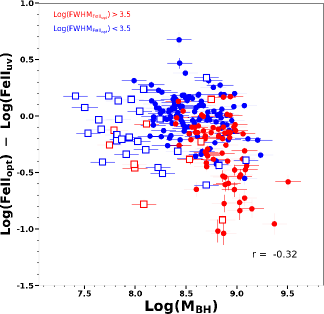
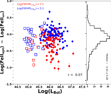
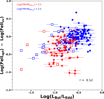
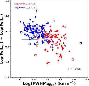
Figure 8.— Comparison of the UV and Optical Fe II emission line fluxes as a function of AGNs properties. Group A ($\rm FWHM_{FeII_{opt}}<10^{3.5}$) is denoted with blue symbols, while Group B ($\rm FWHM_{FeII_{opt}}>10^{3.5}$) is dented with red symbols. Keck and SDSS objects are presented with open and filled symbols, respectively. The correlated coefficients are shown in the lower-left in each panel.

5. Discussion

5.1. Confirmation of systemic velocity shift of the UV and Optical Fe II Emission Lines

One of our main goals in this paper is to confirm the systemic redshift of the optical Fe II emission lines. As we mentioned in Section 1, Sulentic et al. (2012) and Hu et al. (2012) found contrary results on the velocity shift of Fe II_opt emission using a set of composited spectra. Sulentic et al. (2012) generated high S/N composite spectra using the SDSS AGNs, to test the measurement of Hu et al. (2008b). The spectra were binned based on Fe II strengths with a limited range of H$\beta$ FWHM $\leq$ 4000 km s^-1 or H$\beta$ FWHM between $4000$ and $8000$ km s^-1. The composite spectra with high S/N ($\sim$55$-$60) composite spectra did not show a systemic redshift of optical Fe II with respect to [O III]. However, by combining AGNs with the simialr $\rm V_{FeII}$, Hu et al. (2012) argued that their measurement of the systemic redshift was reliable. While these two studies used composite spectra with a very high S/N, which were binned with different criteria, the results lead to discrepancy.

The solution to this issue is to use individual spectra with a high S/N, and we were able to measure the velocity shift of Fe II_opt using a large sample of luminous AGNs with high S/N spectra. In Section 4.1.3, we present the distribution of Fe II_opt (Figure 5), showing that Fe II_opt show a large range of velocity shift with an average $\sim$182 $\pm$ 95 km s^-1. Our results confirmed that optical Fe II emission lines are redshifted on average. The discrepancy between Hu et al. (2008b) and Sulentic et al. (2012) may be caused by the different criteria in constructing composite spectra. Sulentic et al. (2012) combined the spectra over the limited ranges of FWHM of H$\beta$ and Fe II strength, while Hu et al. (2012) combined the spectra based on the limited ranges of Fe II velocity. Hu et al. (2012) argued that Sulentic et al. (2012) failed to find the systemic redshift of Fe II_opt because they made composite spectra using similar FWHM H$\beta$ and Fe II strength, averaging the velocity shift of individual objects.

We also find the average velocity shift of Fe II_uv as 40 $\pm$ 141 km s^-1, which is smaller than that of the previous measurement, 1150 $\pm$ 580 km s^-1 by Kovačević-Dojčinović & Popović (2015). Note that Kovačević-Dojčinović & Popović (2015) mentioned that their measured velocity shift of Fe II_uv should be taken into caution because of large uncertainty for individual AGNs with very broad UV Fe II emission, while it is not clear why the measured average velocity shift of Fe II_uv is different between Kovačević-Dojčinović & Popović (2015) and ours. One possibility is that the difference may be caused by different Fe II templates. In our analysis, we adopted the I Zw 1 Fe II template of Tsuzuki et al. (2006), while Kovačević-Dojčinović & Popović (2015) used the UV Fe II template from Kovačević et al. (2010). Recently, Shin et al. (2019) showed that the flux ratio of Fe II/Mg II could be different up to $\sim$0.2 dex if the flux of Fe II is modeled from different Fe II templates such as Vestergaard & Wilkes (2001) and Tsuzuki et al. (2006).

5.2. Origins of the UV and Optical Fe II Emission Lines

We showed that the widths of Fe II_uv and Fe II_opt  lines are comparable, suggesting that the two emission line regions are close to each other, as reported and suggested by previous studies (Hu et al., 2008b; Kovačević-Dojčinović & Popović, 2015). Interestingly, AGNs in Group A and Group B show a different trend in comparing the widths of Fe II_uv and Fe II_opt. For AGNs with a relatively narrow Mg II line (i.e., $<$ 4000 km s^-1; Group A), the widths of Fe II_uv and Fe II_opt are comparable (Figure 4). In contrast, for AGNs with a very broad Mg II line (i.e., $>$ 4000 km s^-1; Group B), Fe II_opt is broader than Fe II_uv. Similarly, the velocity shifts of Fe II_uv and Fe II_opt are better correlated in Group A, while there is a much larger scatter in Group B. These results suggest that the Fe II emission region is more complex for the AGNs with large gas velocities. Previously, Kovačević-Dojčinović & Popović (2015) reported a large average velocity shift of Fe II_uv, but no significant velocity shift of Fe II_opt. Kovačević-Dojčinović & Popović (2015) discussed that the UV and optical Fe II emission lines may be located in the same region, however, if Fe II_optemitting gas clouds are more symmetrically distributed than UV-emitting gas, potentially causing the difference in the velocity shift. In addition, Kovačević-Dojčinović & Popović (2015) discussed the effect of internal shock waves in the infalling gas. As the shock may contribute the excitation of UV lines, a larger redshift is expected in Fe II_uv.

Following the study of Ferland et al. (2009), who focused on the anisotropic properties of Fe II emission based on a photoionization calculation for a single cloud in the BLR, we consider a couple of effects on the Fe II line emission. First, we expect anisotropy in Fe II emission due to the various contribution from the front illuminated side and the back shielded face of each cloud. It is expected that the anisotropy is stronger for higher column density clouds, and that Fe II_uv emission is emitted more asymmetric since UV Fe II emission arises from larger optical thick transitions compare to that of optical Fe II emission. In contrast, Fe II_opt emission is expected to be more isotropic with symmetry between illuminated and shielded sides of individual clouds. Second, the observed Fe II emission is the combination of the flux from individual clouds with varying column density and distance from the central photoionizing source. As shown by Ferland et al. (2009), clouds with higher column density are expected to have less acceleration due to radiation pressure and show infall signature, i.e., redshifted Fe II emission. Thus, depending on the column density distribution of individual clouds in the BLR, the observed Fe II emission may show different signatures in the velocity shift and line width between the UV and optical Fe II emission lines.

As shown in Figure 8, AGNs in Group A have higher Eddington ratio and higher optical-to-UV Fe II flux ratio than AGNs in group B, indicating that the average column density of individual clouds is higher. Thus, we may expect stronger anisotropy in Fe II emission from individual clouds. Nevertheless, we find no corresponding kinematical signature in Group A in comparison with Group B, since the relative velocity shift between optical and UV Fe II emission is similar between the two groups (see Figure 6). The scatter of the relative velocity shift is even smaller in Group A than in Group B. In the case of the line width, we also see that AGNs in Group A show similar line widths between the optical and UV Fe II emission. These results may imply that the observed velocity shift and line width, which are flux-weighted over a large number of individual clouds, may not be directly influenced by the anisotropy of Fe II emission from each cloud.

While the model of Ferland et al. (2009) has successfully explained the redshift of Fe II (e.g., Hu et al., 2008b, Kovačević-Dojčinović & Popović, 2015), and supports our result that the UV and optical Fe II emission lines are on average redshifted (40 $\pm$ 141 km s^-1 and 182 $\pm$ 95, respectively for Fe II_uv and Fe II_opt, with respect to the peak of the H$\beta$ line), there are also AGNs with blueshifted Fe II, particularly in UV emission. These AGNs may indicate outflows of gas clouds. Note that each cloud in the BLR can be accelerated outward due to strong radiation pressure or infall due to weak acceleration from radiation pressure, depending on the column density of each cloud compared to the minimum column density required for infall (see Equation 2 in Ferland et al., 2009). Thus, for a given AGN, there could be a mix of outflows and infall in the BLR. Without spatially-resolving individual clouds, we only see the average velocity shift of flux-weighted Fe II emission. This scenario may explain our result, which shows a large range of average velocity shift of Fe II (e.g., $\pm$1500 km s^-1).

6. Conclusions

In this paper, we investigate the kinematical properties of the UV and optical Fe II emission lines, using a sample of 223 AGNs at 0.4 $<$ z $<$ 0.8 with a high S/N ratio in the continuum, which allowed us to explore the connection between the UV and optical Fe II emission regions. The main results are summarized as follows:

(1) We find a strong correlation between the widths of UV and optical Fe II emission lines, supporting that both UV and optical Fe II emissions arise from an approximately same distance in the BLR. However, we find a different trend depending on the width of Fe II. The line widths of UV and optical Fe II emission lines are comparable to each other for AGNs with a relatively small Fe II_opt line width (i.e., FWHM $<$ 3200 km s^-1; Group A), while for AGNs with a very broad Fe II_opt (i.e., FWHM $>$ 3200 km s^-1; Group B), Fe II_opt is broader than Fe II_uv.

(2) Fe II emission lines are on average narrower than H$\beta$ and Mg II for Group A, indicating the Fe II emission region is further out in the BLR. This result is consistent with the previous study by Hu et al. (2008b) for the optical Fe II emission. However, for AGNs with very broad Fe II, Fe II_opt emission line is comparable to or broader than H$\beta$ or Mg II.

(3) We confirm the systemic redshift of optical Fe II emission lines with an average velocity 182 $\pm$ 95 km s^-1, as similarly reported by Hu et al. (2008b) and Kovačević-Dojčinović & Popović (2015), while for individual AGNs there is a large range of the velocity shift, including blueshift. In the case of UV Fe II emission lines, we find the average velocity 40 $\pm$ 141 km s^-1. The average velocity shift of the UV and optical Fe II emission may indicate inflow motion. However, there are AGNs with various signs of the velocity shift, indicating complex nature of Fe II emission.

References

- Bae & Woo (2014) Bae, H.-J., & Woo, J.-H. 2014, ApJ, 795, 30
- Bae & Woo (2016) Bae, H.-J., & Woo, J.-H. 2016, ApJ, 828, 97
- Baldwin et al. (2004) Baldwin, J. A., Ferland, G. J., Korista, K. T., Hamann, F., & LaCluyzé, A. 2004, ApJ, 615, 610
- Bennert et al. (2010) Bennert, V. N., Treu, T., Woo, J.-H., et al. 2010, ApJ, 708, 1507
- Bevington & Robinson (2003) Bevington, P. R., & Robinson, D. K. 2003, Data Reduction and Error Analysis for the Physical Sciences (3rd ed.; Boston, MA: McGraw-Hill)
- Boroson & Green (1992) Boroson, T. A., & Green, R. F. 1992, ApJS, 80, 109
- Collin & Joly (2000) Collin, S., & Joly, M. 2000, NewAR, 44, 531
- De Rosa et al. (2011) De Rosa, G., Decarli, R., & Walter, F., et al. 2011, ApJ, 739, 56
- Ferland et al. (2009) Ferland, G. J., Hu, C., Wang, J.-M., et al. 2009, ApJ, 707, 82
- Grandi (1982) Grandi, S. A. 1982, ApJ, 255, 25
- Greene & Ho (2005) Greene, J. E., & Ho, L. C. 2005, ApJ, 630, 122
- Greenstein & Schmidt (1964) Greenstein, J. L., & Schmidt, M. 1964, ApJ, 140, 1
- Dong et al. (2011) Dong, X., Wang, J., Ho, L. C., et al. 2011, ApJ, 736, 86
- Joly (1987) Joly, M. 1987, A&A, 184, 33
- Kim et al. (2006) Kim, M., Ho, L. C., & Im, M. 2006, ApJ, 642, 702
- Kovačević et al. (2010) Kovačević, J., Popović, L. Č, & Dimitrijević, M. S. 2010, ApJS, 189, 15
- Kovačević-Dojčinović & Popović (2015) Kovačević-Dojčinović, J., & Popović, L. Č. 2015, ApJS, 221, 35
- Kovačević et al. (2014) Kovačević-Dojčinović, J., Popović, L. Č., & Kollatschny, W. 2017, arXiv:1311.6653
- Kovačević-Dojčinović et al. (2017) Kovačević-Dojčinović, J., Marčeta-Mandič, S., & Popović, L. Č. 2017, arXiv:1707.08251
- Kwan & Krolik (1981) Kwan, J., & Krolik, J. H. 1981, ApJ, 250, 478
- Lipari & Terlevich (2006) Lipari, S. L., & Terlevich, R. J. 2006, MNRAS, 368, 1001
- Markwardt (2009) Markwardt, C. B. 2009, in Astronomical Data Analysis Software and Systems XVIII, ed. D. A. Bohlender, D. Durand, & P. Dowler (San Francisco: ASP), 251
- McGill et al. (2008) McGill, K. L., Woo, J.-H., Treu, T., & Malkan, M. A. 2008, ApJ, 673, 703
- Oke et al. (1995) Oke, J. B., Cohen, J. G., Carr, M., et al. 1995, PASP, 107, 375
- Park et al. (2015) Park, D., Woo, J.-H., Bennert, V. et al. 2015, ApJ, 799, 164
- Popović et al. (2003) Popović, L. Ć., Mediavilla, E. G., Bon, E., Stanič, N., & Kubićela, A. 2003, ApJ, 599, 185
- Popović et al. (2007) Popović, L. Ć., Smirnova, A., Ilić, D., Moiseev, A.,Kovačević, J., & Afanasiev, V. 2007, in The Central Engine of Active Galactic Nuclei, ed. L. C. Ho & J. -M. Wang (San Francisco: ASP), 552
- Rakshit & Woo (2018) Rakshit, S., & Woo, J. -H. 2017, ApJ, 865, 5
- Sameshima et al. (2011) Sameshima, H., Kawara, K., Matsuoka, Y., et al. 2011, MNRAS, 410, 1018
- Sameshima et al. (2017) Sameshima, H., Yoshii, Y., & Kawara, K. 2017, ApJ, 834, 203
- Sani et al. (2010) Sani, E., Lutz, D., Risaliti, G., et al. 2010, MNRAS, 403, 1246
- Schlegel et al. (1998) Schlegel, D. J., Finkbeiner, D. P., & Davis, M. 1998, ApJ, 500, 525
- Shin et al. (2019) Shin, J., Nagao, T., Woo, J. -H., & Le, H. A. N. 2019, ApJ, 874, 1
- Shen et al. (2011) Shen, Y., Richards, G. T., Strauss, M. A., et al. 2011, ApJS, 194, 45
- Sulentic et al. (2012) Sulentic, J. W., Marziani, P., Zamfir, S., & Meadows, A. 2012, ApJL, 752, L7
- Hu et al. (2008a) Hu, C., Wang, J.-M., Ho, L. C., et al. 2008a, ApJ, 683, L115
- Hu et al. (2008b) Hu, C., Wang, J.-M., Ho, L. C., et al. 2008b, ApJ, 687, 78
- Hu et al. (2012) Hu, C., Wang, J.-M., Ho, L. C., et al. 2012, ApJ, 760, 126
- Treu et al. (2004) Treu, T., Malkan, M. A., & Blandford, R. D. 2004, ApJ, 615, L97
- Tsuzuki et al. (2006) Tsuzuki, Y., Kawara, K., Yoshii, Y., et al. 2006, ApJ, 650, 57
- Valdes et al. (2004) Valdes, F., Gupta, R., Rose, J. A., Singh, H. P., & Bell, D. J. 2004, ApJS, 152, 251
- Vestergaard & Wilkes (2001) Vestergaard, M., & Wilkes, B. J. 2001, ApJS, 134, 1
- Wampler & Oke (1967) Wampler, E. J., & Oke, J. B. 1967, ApJ, 148, 695
- Wang et al. (2009) Wang, J.-G., Dong, X.-B., Wang, T.-G., et al. 2009, ApJ, 707, 1334
- Woo et al. (2006) Woo, J.-H., Treu, T., Malkan, M. A., & Blandford, R. D. 2006, ApJ, 645, 900
- Woo (2008) Woo, J.-H. 2008, AJ, 135, 1849
- Woo et al. (2015) Woo, J.-H., Yoon, Y., Park, S. et al. 2015, ApJ, 801, 38
- Woo et al. (2016) Woo, J.-H., Bae, H.-J., Son, D., & Karouzos, M. 2016, ApJ, 817, 108
- Woo et al. (2017) Woo, J.-H., Son, D., & Bae, H.-J. 2017, ApJ, 839, 120
- Woo et al. (2018) Woo, J.-H., Le, H. A. N., Karouzos, M. 2018, ApJ, 859, 138