ACL’20
Not All Claims are Created Equal:
Choosing the Right Statistical Approach to Assess Hypotheses

Abstract

Empirical research in Natural Language Processing (NLP) has adopted a narrow set of principles for assessing hypotheses, relying mainly on $p$-value computation, which suffers from several known issues. While alternative proposals have been well-debated and adopted in other fields, they remain rarely discussed or used within the NLP community. We address this gap by contrasting various hypothesis assessment techniques, especially those not commonly used in the field (such as evaluations based on Bayesian inference). Since these statistical techniques differ in the hypotheses they can support, we argue that practitioners should first decide their target hypothesis before choosing an assessment method. This is crucial because common fallacies, misconceptions, and misinterpretation surrounding hypothesis assessment methods often stem from a discrepancy between what one would like to claim versus what the method used actually assesses. Our survey reveals that these issues are omnipresent in the NLP research community. As a step forward, we provide best practices and guidelines tailored towards NLP research, as well as an easy-to-use package called HyBayes for Bayesian assessment of hypotheses, complementing existing tools.

1 Introduction

Empirical fields, such as Natural Language Processing (NLP), must follow scientific principles for assessing hypotheses and drawing conclusions from experiments. For instance, suppose we come across the results in Table 1, summarizing the accuracy of two question-answering (QA) systems $S_{1}$ and $S_{2}$ on some datasets. What is the correct way to interpret this empirical observation in terms of the superiority of one system over another? While $S_{1}$ has higher accuracy than $S_{2}$ in both cases, the gap is moderate and the datasets are of limited size. Can this apparent difference in performance be explained simply by random chance, or do we have sufficient evidence to conclude that $S_{1}$ is in fact inherently different (in particular, inherently stronger) than $S_{2}$ on these datasets? If the latter, can we quantify this gap in inherent strength while accounting for random fluctuation?

System	Description	ARC-easy		ARC-challenge
ID		#Correct	Acc.	#Correct	Acc.
$S_{1}$	BERT	1721	72.4	566	48.3
$S_{2}$	Reading Strategies	1637	68.9	496	42.3

Table 1: Performance of two systems Devlin et al. (2019); Sun et al. (2018) on the ARC question-answering dataset Clark et al. (2018). ARC-easy & ARC-challenge have $2376$ & $1172$ instances, respectively. Acc.: accuracy as a percentage.

Such fundamental questions arise in one form or another in every empirical NLP effort. Researchers often wish to draw conclusions such as:

These two conclusions differ in two respects. First, Ca claims the two systems are inherently different, while Cb goes further to claim a margin of at least 1% between their inherent accuracies. The second, more subtle difference lies in the interpretation of the 95% figure: the 95% confidence expressed in Ca is in terms of the space of empirical observations we could have made, given some underlying truth about how the inherent accuracies of $S_{1}$ and $S_{2}$ relate; while the 95% probability expressed in Cb is directly over the space of possible inherent accuracies of the two systems.

To support such a claim, one must turn it into a proper mathematical statement that can be validated using a statistical calculation. This in turn brings in additional choices: we can make at least four statistically distinct hypotheses here, each supported by a different statistical evaluation:

As this illustrates, there are multiple ways to formulate empirical hypotheses and support empirical claims. Since each hypothesis starts with a different assumption and makes a (mathematically) different claim, it can only be tested with a certain set of statistical methods. Therefore, NLP practitioners ought to define their target hypothesis before choosing an assessment method.

The most common statistical methodology used in NLP is null-hypothesis significance testing (NHST) which uses $p$-values Søgaard et al. (2014); Koehn (2004); Dror and Reichart (2018). Hypotheses H1&H2 can be tested with $p$-value-based methods, which include confidence intervals and operate over the probability space of observations (§2.1 and §2.2). On the other hand, there are often overlooked approaches, based on Bayesian inference Kruschke and Liddell (2018), that can be used to assess hypotheses H3&H4 (§2.3 and §2.4) and have two broad strengths: they can deal more naturally with accuracy margins and they operate directly over the probability space of inherent accuracy (rather than of observations).

For each technique reviewed in this work, we discuss how it compares with alternatives and summarize common misinterpretations surrounding it (§3). For example, a common misconception about $p$-value is that it represents a probability of the validity of a hypothesis. While desirable, $p$-values in fact do not provide such a probabilistic interpretation (§3.2). It is instead through a Bayesian analysis of the posterior distribution of the test statistic (inherent accuracy in the earlier example) that one can make claims about the probability space of that statistic, such as H3.

We quantify and demonstrate related common malpractices in the field through a manual annotation of 439 ACL-2018 conference papers, and a survey filled out by 55 NLP researchers (§4). We highlight surprising findings from the survey, such as the following: While 86% expressed fair-to-complete confidence in the interpretation of $p$-values, only a small percentage of them correctly answered a basic $p$-value interpretation question.

Contributions.

This work seeks to inform the NLP community about crucial distinctions between various statistical hypotheses and their corresponding assessment methods, helping move the community towards well-substantiated empirical claims and conclusions. Our exposition covers a broader range of methods (§2) than those included in recent related efforts (§1.1), and highlights that these methods achieve different goals. Our surveys of NLP researchers reveals problematic trends (§4), emphasizing the need for increased scrutiny and clarity. We conclude by suggesting guidelines for better testing (§5), as well as providing a toolkit called HyBayes (cf. Footnote 1) tailored towards commonly used NLP metrics. We hope this work will encourage an improved understanding of statistical assessment methods and effective reporting practices with measures of uncertainty.

1.1 Related Work

While there is an abundant discussion of significance testing in other fields, only a handful of NLP efforts address it. For instance, Chinchor (1992) defined the principles of using hypothesis testing in the context of NLP problems. Most-notably, there are works studying various randomized tests Koehn (2004); Ojala and Garriga (2010); Graham et al. (2014), or metric-specific tests Evert (2004). More recently, Dror et al. (2018) and Dror and Reichart (2018) provide a thorough review of frequentist tests. While an important step in better informing the community, it covers a subset of statistical tools. Our work complements this effort by pointing out alternative tests.

With increasing over-reliance on certain hypothesis testing techniques, there are growing troubling trends of misuse or misinterpretation of such techniques Goodman (2008); Demšar (2008). Some communities, such as statistics and psychology, even have published guidelines and restrictions on the use of $p$-values Trafimow and Marks (2015); Wasserstein et al. (2016). In parallel, some authors have advocated for using alternate paradigms such as Bayesian evaluations Kruschke (2010).

NLP is arguably an equally empirical field, yet with a rare discussion of proper practices of scientific testing, common pitfalls, and various alternatives. In particular, while limitations of $p$-values are heavily discussed in statistics and psychology, only a few NLP efforts approach them: over-estimation of significance by model-based tests Riezler and Maxwell (2005), lack of independence assumption in practice Berg-Kirkpatrick et al. (2012), and sensitivity to the choice of the significance level Søgaard et al. (2014). Our goal is to provide a unifying view of the pitfalls and best practices, and equip NLP researchers with Bayesian hypothesis assessment approaches as an important alternative tool in their toolkit.

2 Assessment of Hypotheses

We often wish to draw qualitative inferences based on the outcome of experiments (for example, inferring the relative inherent performance of systems). To do so, we usually formulate a hypothesis that can be assessed through some analysis.

Suppose we want to compare two systems on a dataset of instances $\boldsymbol{x}=[x_{1},\ldots,x_{n}]$ with respect to a measure $\mathcal{M}(S,x)$ representing the performance of a system $S$ on an instance $x$. Let $\mathcal{M}(S,\boldsymbol{x})$ denote the vector $[\mathcal{M}(S,{x}_{i})]_{i=1}^{n}$. Given systems $S_{1},S_{2}$, define $\boldsymbol{y}\triangleq[\mathcal{M}(S_{1},\boldsymbol{x}),\mathcal{M}(S_{2},\boldsymbol{x})]$ as a vector of observations.

In a typical NLP experiment, the goal is to infer some inherent and unknown properties of systems. To this end, a practitioner assumes a probability distribution on the observations $\boldsymbol{y}$, parameterized by $\boldsymbol{\theta}$, the properties of the systems. In other words, $\boldsymbol{y}$ is assumed to have a distribution with unknown parameters $\boldsymbol{\theta}$. In this setting, a hypothesis $H$ is a condition on $\boldsymbol{\theta}$. Hypothesis assessment is a way of evaluating the degree to which the observations $\boldsymbol{y}$ are compatible with $H$. The overall process is depicted in Figure 1.

Figure 1: Progression of steps taken during a scientific assessment of claims from empirical observations.

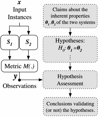
Following our running example, we use the task of answering natural language questions Clark et al. (2018). While our examples are shown for this particular task, all the ideas are applicable to more general experimental settings.

For this task, the performance metric $\mathcal{M}(S,x)$ is defined as a binary function indicating whether a system $S$ answers a given question $x$ correctly or not. The performance vector $\mathcal{M}(S,\boldsymbol{x})$ captures the system’s accuracy on the entire dataset (cf. Table 1). We assume that each system $S_{i}$ has an unknown inherent accuracy value, denoted $\theta_{i}$. Let $\boldsymbol{\theta}=[\theta_{1},\theta_{2}]$ denote the unknown inherent accuracy of two systems. In this setup, one might, for instance, be interested in assessing the credibility of the hypothesis $H$ that $\theta_{1}<\theta_{2}$.

Table 2: Various classes of methods for statistical assessment of hypotheses.

Table 2 shows a categorization of statistical tools developed for the assessment of such hypotheses. The two tools on the left are based on frequentist statistics, while the ones on the right are based on Bayesian inference Kruschke and Liddell (2018). A complementary categorization of these tools is based on the nature of the results that they provide: the ones on the top encourage binary decision making, while those on the bottom provide uncertainty around estimates. We discuss all four classes of tests in the following sub-sections.

2.1 Null-Hypothesis Significance Testing

In frequentist hypothesis testing, there is an asymmetric relationship between two hypotheses. The hypothesis formulated to be rejected is usually called the null-hypothesis $H_{0}$. For instance, in our example $H_{0}$$:\theta_{1}=\theta_{2}$. A decision procedure is devised by which, depending on $\boldsymbol{y}$, the null-hypothesis will either be rejected in favor of $H_{1}$, or the test will stay undecided.

A key notion here is $p$-value, the probability, under the null-hypothesis $H_{0}$, of observing an outcome at least equal to or extreme than the empirical observations $\boldsymbol{y}$. To apply this notion on a set of observations $\boldsymbol{y}$, one has to define a function that maps $\boldsymbol{y}$ to a numerical value. This function is called the test statistic $\delta(.)$ and it formalizes the interpretation of extremeness. Concretely, $p$-value is defined as,

$$\mathbb{P}(\delta(Y)\geq\delta(\boldsymbol{y})|\emph{$H_{0}$})$$ (1)

In this notation, $Y$ is a random variable over possible observations and $\delta(\boldsymbol{y})$ is the empirically observed value of the test statistic.

A large $p$-value implies that the data could easily have been observed under the null-hypothesis. Therefore, a lower $p$-value is used as evidence towards rejecting the null-hypothesis.

Example 1 (Assessment of H1)

We form a null-hypothesis using the accuracy of the two systems (Table 1) using a one-sided $z$-test with $\delta(\boldsymbol{y})\triangleq(1/n)\sum_{i=1}^{n}\left[\mathcal{M}({S}_{1},x_{i})-\mathcal{M}({S}_{2},x_{i})\right].$ We formulate a null-hypothesis against the claim of ${S}_{1}$ having strictly better accuracy than ${S}_{2}$. This results in a $p$-value of $0.0037$ (details in §A.1) and can be interpreted as the following: if the systems have inherently identical accuracy values, the probability of observing a superiority at least as extreme as our observations is $0.0037$. For a significance level of $0.05$ (picked before the test) this $p$-value is small enough to reject the null-hypothesis.

This family of the tests is thus far the most widely used tool in NLP research. Each variant of this test is based on some assumptions about the distribution of the observations, under the null-hypothesis, and an appropriate definition of the test statistics $\delta(.)$. Since a complete exposition of such tests is outside the scope of this work, we encourage interested readers to refer to the existing reviews, such as Dror et al. (2018).

2.2 Confidence Intervals

Confidence Intervals (CIs) are used to express the uncertainty of estimated parameters. In particular, the $95$% CI is the range of values for parameter $\boldsymbol{\theta}$ such that the corresponding test based on $p$-value is not rejected:

$$\mathbb{P}(\delta(Y)\geq\delta(\boldsymbol{y})|\emph{$H_{0}$}(\boldsymbol{\theta}))\geq 0.05.$$ (2)

In other words, the confidence interval merely asks which values of the parameter $\boldsymbol{\theta}$ could be used, before the test is rejected.

Example 2 (Assessment of H2)

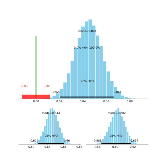
Consider the same setting as in Example 1. According to Table 1, the estimated value of the accuracy differences (maximum-likelihood estimates) is $\theta_{1}-\theta_{2}=0.035$. A 95% CI of this quantity provides a range of values that are not rejected under the corresponding null-hypothesis. In particular, a 95% CI gives $\theta_{1}-\theta_{2}\in[0.0136,0.057]$ (details in §A.2). The blue bar in Figure 2 (right) shows the corresponding CI. Notice that the conclusion of Example 1 is compatible with this CI; the null-hypothesis $\theta_{1}=\theta_{2}$ which got rejected is not included in the CI.

2.3 Posterior Intervals

Bayesian methods focus on prior and posterior distributions of $\boldsymbol{\theta}$. Recall that in a typical NLP experiment, these parameters can be, e.g., the actual mean or standard deviation for the performance of a system, as its inherent and unobserved property.

In Bayesian inference frameworks, a priori assumptions and beliefs are encoded in the form of a prior distribution $\mathbb{P}(\boldsymbol{\theta})$ on parameters of the model. In other words, a prior distribution describes the common belief about the parameters of the model. It also implies a distribution over possible observations. For assessing hypotheses H3 and H4 in our running example, we will simply use the uniform prior, i.e., the inherent accuracy is uniformly distributed over $[0,1]$. This corresponds to having no prior belief about how high or low the inherent accuracy of a typical QA system may be.

In general, the choice of this prior can be viewed as a compromise between the beliefs of the analyzer and those of the audience. The above uniform prior, which is equivalent to the Beta(1,1) distribution, is completely non-committal and thus best suited for a broad audience who has no reason to believe an inherent accuracy of 0.8 is more likely than 0.3. For a moderately informed audience that already believes the inherent accuracy is likely to be widely distributed but centered around 0.67, the analyzer may use a Beta(3,1.5) prior to evaluate a hypothesis. Similarly, for an audience that already believes the inherent accuracy to be highly peaked around 0.75, the analyzer may want to use a Beta(9,3) prior. Formally, one incorporates $\boldsymbol{\theta}$ in a hierarchical model in the form of a likelihood function $\mathbb{P}(\boldsymbol{y}|\boldsymbol{\theta})$. This explicitly models the underlying process that connects the latent parameters to the observations. Consequently, a posterior distribution is inferred using the Bayes rule and conditioned on the observations: $\mathbb{P}(\boldsymbol{\theta}|\boldsymbol{y})=\frac{\mathbb{P}(\boldsymbol{y}|\boldsymbol{\theta})\mathbb{P}(\boldsymbol{\theta})}{\mathbb{P}(\boldsymbol{y})}.$

The posterior distribution is a combined summary of the data and prior information, about likely values of $\boldsymbol{\theta}$. The mode of the posterior (maximum a posteriori) can be seen as an estimate for $\boldsymbol{\theta}$. Additionally, the posterior can be used to describe the uncertainty around the mode.

While the posterior distribution can be analytically calculated for simple models, it is not so straightforward for general models. Fortunately, recent advances in hardware, Markov Chain Monte Carlo (MCMC) techniques Metropolis et al. (1953); Gamerman and Lopes (2006), and probabilistic programming allow sufficiently-accurate numerical approximations of posteriors.

Figure 2: Left: Prior distributions of two systems (bottom row) and their difference (top row). Right: Posterior distributions of two systems (bottom row) and their difference (top row) after observing the performances on ARC-easy dataset. Note the posterior HDI estimate, $(0.00939,0.0612)$. Here we assume at least one percent accuracy difference to be considered practically different. Hence, we indicate the interval $(-0.01,0.01)$ as ROPE (§2.3.)

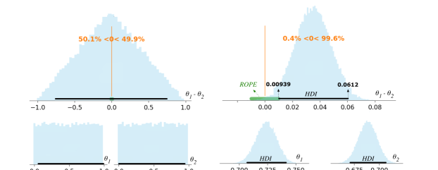
One way to summarize the uncertainty around the point estimate of parameters is by marking the span of values that cover $\alpha$% of the most-credible density in the posterior distribution (e.g., $\alpha=95$%). This is called Highest Density Intervals (HDIs) or Bayesian Confidence Intervals Oliphant (2006) (not to be confused with CI, in §2.2).

Recall that a hypothesis $H$ is a condition on $\boldsymbol{\theta}$ (see Figure 1). Therefore, given the posterior $\mathbb{P}(\boldsymbol{\theta}|\boldsymbol{y})$, one can calculate the probability of $H$, as a probabilistic event, conditioned on $\boldsymbol{y}$: $\mathbb{P}(H|\boldsymbol{y})$.

For example in an unpaired $t$-test, $H_{0}$ is the event that the means of two groups are equal. Bayesian statisticians usually relax this strict equality $\theta_{1}=\theta_{2}$ and instead evaluate the credibility of $|\theta_{1}-\theta_{2}|<\varepsilon$ for some small value of $\varepsilon$. The intuition is that when $\theta_{1}$ and $\theta_{2}$ are close enough they are practically equivalent. This motivates the definition of Region Of Practical Equivalence (ROPE): An interval around zero with “negligible” radius. The boundaries of ROPE depend on the application, the meaning of the parameters and its audience. In our running example, a radius of one percent for ROPE implies that improvements less than $1$ percent are not considered notable. For a discussion on setting ROPE see Kruschke (2018).

These concepts give researchers the flexibility to define and assess a wide range of hypotheses. For instance, we can address H3 (from Introduction) and its different variations that can be of interest depending on the application. The analysis of H3 is depicted in Figure 2 and explained next.

Example 3 (Assessment of H3)

Recall the setting from previous examples. The left panel of Figure 2 shows the prior on the latent accuracy of the systems and their differences (further details on the hierarchical model in §A.3.) We then obtain the posterior distribution (Figure 2, right), in this case via numerical methods). Notice that one can read the following conclusion: with probability $0.996$, the hypothesis H3 (with a margin of 0%) holds true. As explained in §C.2, this statement does not imply any difference with a notable margin. In fact, the posterior in Figure 2 implies that this experiment is not sufficient to claim the following: with probability at least $0.95$, hypothesis H3 (with a margin of 1%) holds true. This is the case since ROPE $(−0.01,0.01)$ overlaps with $95\%$ HDI $(0.00939,0.0612).$

2.4 Bayes Factor

A common tool among Bayesian frameworks is the notion of Bayes Factor. Intuitively, it compares how the observations $\boldsymbol{y}$ shift the credibility from prior to posterior of the two competing hypothesis:

$$\mathit{BF}_{01}=\frac{\mathbb{P}(\text{$H_{0}$}|\boldsymbol{y})}{\mathbb{P}(\text{$H_{1}$}|\boldsymbol{y})}\Bigg{/}\frac{\mathbb{P}(\text{$H_{0}$})}{\mathbb{P}(\text{$H_{1}$})}$$

If the $\mathit{BF}_{01}$ equals to 1 then the data provide equal support for the two hypotheses and there is no reason to change our a priori opinion about the relative likelihood of the two hypotheses. A smaller Bayes Factor is an indication of rejecting the null-hypothesis $H_{0}$. If it is greater than 1 then there is support for the null-hypothesis and we should infer that the odds are in favor of $H_{0}$.

Notice that the symmetric nature of Bayes Factor allows all the three outcomes of “accept”, “reject”, and “undecided,” as opposed to the definition of $p$-value that cannot accept a hypothesis.

Example 4 (Assessment of H4)

Here we want to assess the null-hypothesis $H_{0}$: $|\theta_{1}-\theta_{2}|<0.01$ against $H_{1}$: $|\theta_{1}-\theta_{2}|\geq 0.01$ ($x=0.01$). Substituting posterior and prior values, one obtains: $$\mathit{BF}_{01}=\frac{0.027}{0.980}\Bigg{/}\frac{0.019}{0.972}=1.382$$ . This value is very close to $1$ which means that this observation does not change our prior belief about the two systems difference.

3 Comparisons

Many aspects influence the choice of an approach to assess significance of hypotheses. This section provides a comparative summary, with details in Appendix C and an overall summary in Table 3.

Method	Paradigm	Ease of interpretation ($1=$easy) (§3.1)	Encourages binary-thinking (3.2)	Depends on stopping intention (3.3)	Dependence on prior (3.4)	Decision rule	# of papers using this test in ACL’18
(§2.1) $p$-value	frequentist	3	Yes	Yes	No	Acceptable $p$-value	73
(§2.2) CI	frequentist	4	No	Yes	No	Acceptable confidence margin	6
(§2.3) HDI	Bayesian	1	No	No	Not sensitive but takes it into account	HDI relative to ROPE	0
(§2.4) BF	Bayesian	2	Yes	No	Highly sensitive	Acceptable BF	0

Table 3: A comparison of different statistical methods for evaluating the credibility of a hypothesis given a set of observations. The total number of published papers in at the ACL-2018 conference is 439.

3.1 Susceptibility to Misinterpretation

The complexity of interpreting significance tests combined with insufficient reporting could result in ambiguous or misleading conclusions. This ambiguity can not only confuse authors but also cause confusion among readers of the papers.

While $p$-values (§2.1) are the most common approach, they are inherently complex, which makes them easier to misinterpret (see examples in §C.1). Interpretation of confidence intervals (§2.2) can also be challenging since it is an extension of $p$-value Hoekstra et al. (2014). Approaches that provide measures of uncertainty directly in the hypothesis space (like the ones in §2.3) are often more natural choices for reporting the results of experiments Kruschke and Liddell (2018).

3.2 Measures of Certainty

A key difference is that not all methods studied here provide a measure of uncertainty over the hypothesis space. For instance, $p$-values (§2.1) do not provide probability estimates on two systems being different (or equal) Goodman (2008). On the contrary, they encourage binary thinking Gelman (2013), that is, confidently concluding that one system is better than another, without taking into account the extent of the difference between the systems. CIs (§2.2) provide a range of values for the target parameter. However, this range also does not have any probabilistic interpretation in the hypothesis space du Prel et al. (2009). On the other hand, posterior intervals (§2.3) generally provide a useful summary as they capture probabilistic estimates of the correctness of the hypothesis.

3.3 Dependence on Stopping Intention

The process by which samples in the test are collected can affect the outcome of a test. For instance, the sample size $n$ (whether it is determined before the process of gathering information begins, or is a random variable itself) can change the result. Once observations are recorded, this distinction is usually ignored. Hence, the testing algorithms that do not depend on the distribution of $n$ are more desirable. Unfortunately, the definition of $p$-value (§2.1) depends on the distribution of $n$. For instance, Kruschke (2010, §11.1) provides examples where this subtlety can change the outcome of a test, even when the final set of observations is identical.

3.4 Sensitivity to the Choice of Prior

The choice of the prior can change the outcome of Bayesian approaches (§2.3 & §2.4). Decisions of Bayes Factor (§2.4) are known to be sensitive to the choice of prior, while posterior estimates (§2.3) are less so. For further discussion, see C.4 or refer to discussions by Sinharay and Stern (2002); Liu and Aitkin (2008) or Dienes (2008).

4 Current Trends and Malpractices

This section highlights common practices relevant to the our target approaches. To better understand the common practices or misinterpretations in the field, we conducted a survey. We shared the survey among $\sim$450 NLP researchers (randomly selected from ACL’18 Proceedings) from which 55 individuals filled out the survey. While similar surveys have been performed in other fields Windish et al. (2007), this is the first in the NLP community, to the best of our knowledge. Here we review the main highlights (see Appendix for more details and charts).

Interpreting $p$-values.

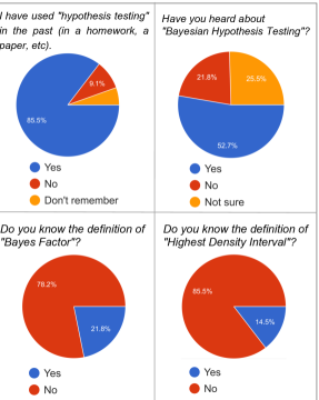
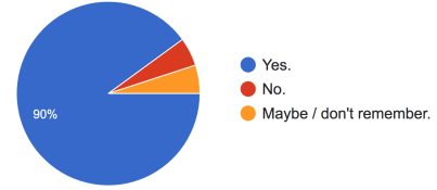
While the majority of the participants have a self-claimed ability to interpret $p$-values (Figure 9(f)), many choose its imprecise interpretation “The probability of the observation this extreme happening due to pure chance” (the popular choice) vs. a more precise statement “Conditioned on the null hypothesis, the probability of the observation this extreme happening.” (see Q1 & Q2 in Appendix B.)

The use of CIs.

Even though $95\%$ percent of the participants self-claimed the knowledge of CIs (Figure 9(e)), it is rarely used in practice. In an annotation done on ACL’18 papers by two of the authors, only 6 (out of 439) papers were found to use CIs.

The use of Bayes Factors.

A majority of the participants had “heard” about “Bayesian Hypothesis Testing” but did not know the definition of “Bayes Factor” (Figure 3). HDIs (discussed in §2.3) were the least known. We did not find any papers in ACL’18 that use Bayesian tools.

The use of “significan*”.

A notable portion of NLP papers express their findings by using the term “significant” (e.g., “our approach significantly improves over X.”) Almost all ACL’18 papers use the term “significant” somewhere. Unfortunately, there is no single universal interpretation of such phrases across readers. In our survey, we observe that when participants read “X significantly improves Y” in the abstract of a hypothetical paper:

1. About $82\%$ expect the claim to be backed by “hypothesis testing”; however, only $57\%$ expect notable empirical improvement (see Q3 in Appendix B);

2. About $35\%$ expect the paper to test “practical significance”, which is not generally assessed by popular tests (see §C.2);

3. A few also expect a theoretical argument.

Figure 3: Select results from our survey.

Recent trends.

Table 3 provides a summary of the techniques studied here. We make two key observations: (i) many papers don’t use any hypothesis assessment method and would benefit from one; (ii) from the final column, $p$-value based techniques clearly dominate the field, a clear disregard to the advantages that the bottom two alternatives offer.

5 Recommended Practices

Having discussed common issues, we provide a collection of recommendations (in addition to the prior recommendations, such as by Dror et al. (2018)).

The first step is to define your goal. Each of the tools in §2 provides a distinct set of information. Therefore, one needs to formalize a hypothesis and consequently the question you intend to answer by assessing this hypothesis. Here are four representative questions, one for each method:

Table 4: Select models supported by our package HyBayes at the time of this publication.

If you decide to use frequentist tests:

• Check if your setting is compatible with the assumptions of the test. In particular, investigate if the meaning of null-hypothesis and sampling distribution match the experimental setting.

• Include a summary of the above investigation. Justify unresolved assumption mismatches.

• Statements reporting $p$-value and confidence interval must be precise enough so that the results are not misinterpreted (see §3.1).

• The term “significant” should be used with caution and clear purpose to avoid misinterpretations (see §4). One way to achieve this is by using adjectives “statistical” or “practical” before any (possibly inflected) usage of “significance.”

• Often times, the desired conclusion is a notable margin in the superiority of one system over another (see §3). In such cases, a pointwise $p$-value argument is not sufficient; a confidence interval analysis is needed. If CI is inapplicable for some reason, this should be mentioned.

If you decide to use Bayesian approaches:

• Since Bayesian tests are less known, it is better to provide a short motivation for the usage.

• Familiarize yourself with packages that help you decide a hierarchical model, e.g., the software provided here. If necessary, customize these models for your specific problem.

• Be clear about your hierarchical model, including model parameters and priors. In most cases, these choices should be justified (see §2.3.)

• Comment on the certainty (or the lack of) of your inference in terms of HDI and ROPE: (I) is HDI completely inside ROPE, (II) they are completely disjoint, (III) HDI contains values both inside and outside ROPE (see §2.3.)

• For reproducibility, include further details about your test: MCMC traces, convergence plots, etc. (Our HyBayes package provides all of this.)

• Be wary that Bayes Factor is highly sensitive to the choice of prior (see §3.4). See Appendix §C.4 for possible ways to mitigate this.

5.1 Package HyBayes

We provide an accompanying package, HyBayes, to facilitate comparing systems using the two Bayesian hypothesis assessment approaches discussed earlier: (a) posterior probabilities and (b) Bayes Factors. (Several packages are already available for frequentist assessments.)

Table 4 summarizes common settings in which HyBayes can be employed in NLP research, including typical use cases, underlying data assumptions, recommended hierarchical model, metrics (accuracy, exact match, etc.), and frequentist tests generally used in these cases. These settings cover several typical assumptions on observed NLP data. However, if a user has specific information on observations or can capitalize on other assumptions, we recommend adding a custom model, which can be done relatively easily.

6 Conclusion

Using well-founded mechanisms for assessing the validity of hypotheses is crucial for any field that relies on empirical work. Our survey indicates that the NLP community is not fully utilizing scientific methods geared towards such assessment, with only a relatively small number of papers using such methods, and most of them relying on $p$-value.

Our goal was to review different alternatives, especially a few often ignored in NLP. We surfaced various issues and potential dangers of careless use and interpretations of different approaches. We do not recommend a particular approach. Every technique has its own weaknesses. Hence, a researcher should pick the right approach according to their needs and intentions, with a proper understanding of the techniques. Incorrect use of any technique can result in misleading conclusions.

We contribute a new toolkit, HyBayes, to make it easy for NLP practitioners to use Bayesian assessment in their efforts. We hope that this work provides a complementary picture of hypothesis assessment techniques for the field and encourages more rigorous reporting trends.

Acknowledgments

The authors would like to thank Rotem Dror, Jordan Kodner, and John Kruschke for invaluable feedback on an early version of this draft. This work was partly supported by a gift from the Allen Institute for AI and by DARPA contracts FA8750-19-2-1004 and FA8750-19-2-0201.

Appendix A Additional Details: Examples

A.1 More Details: Example 1

Here we use a one-sided z-test to compare $s_{1}=1721$ out of $2376$ vs $s_{2}=1637$ out of $2376$. We start with calculating the z-score:

$$s_{1}=1721,n_{1}=2376$$ (3)

$$s_{2}=1637,n_{2}=2376$$ (4)

$$p_{1}=s_{1}/n_{1}=0.72432$$ (5)

$$p_{2}=s_{2}/n_{2}=0.68897$$ (6)

$$\tilde{p}=(s_{1}+s_{2})/(n_{1}+n_{2})=0.70664$$ (7)

$$z=\frac{p_{1}-p_{2}}{\sqrt{\tilde{p}(1-\tilde{p})((1/n_{1})+(1/n_{2}))}}=2.676$$ (8)

Then we can read one-sided tail probability from a z-score table corresponding to $2.676$ as $0.00372$.

A.2 More Details: Example 2

Let $\tilde{z}$ denote the z-score corresponding to 95%, i.e., $\tilde{z}=1.644853$. Also, let $s$ be denominator of the z-score formula above, i.e., $\sigma=\sqrt{\tilde{p}(1-\tilde{p})((1/n_{1})+(1/n_{2}))}$. Then the confidence interval is calculated as follows:

$$[p_{1}-p_{2}-\tilde{z}\sigma,p_{1}-p_{2}+\tilde{z}\sigma]=[0.0136,0.057].$$

A.3 More Details: Example 3

Hierarchical model.

In this analysis, the input consists of four non-negative positive integers $a_{1},n_{1},a_{2},$ and $n_{2}$. The $i$th algorithm has answered $a_{i}$(out of $n_{i}$) questions correctly. In our model, we assume that $a_{i}$ follows a binomial distribution with parameters $\theta_{i}$ and $n_{i}$. Note that this is mathematically the same as considering $n_{i}$ Bernoulli random variables with $a_{i}$ of them being success and $n_{i}-a_{i}$ being failure.

Figure 4: The hierarchical model in Example 3&4.

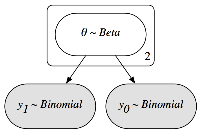
At the higher level, $\theta_{i}$ is assumed to follow a uniform distribution in $[0,1]$. In a later section below, we show how slightly different values for $Beta$ distribution can be used instead as a generalization. To run this analysis with HyBayes one can run the following command:

python -m HyBayes \
       --config config_QABinomial.ini

where config_QABinomial.ini is a configuration file that defines a hierarchical model and the locations of the observations. This particular config file corresponds to the 2nd row of Table 4. For more information and examples, please refer to the manual of our released package (footnote 1).

With this command, HyBayes would run a sampling-based Bayesian inference on the observed data, using the specified hierarchical model. The results should look like Fig. 2.

Generalizations.

It is possible to take previous observations in the literature into account and start with a non-uniform prior. For example, setting $\alpha$ and $\beta$ to $\frac{1}{2}$ incorporates the idea that the performances are generally closer to $0$ or $1$, on the other hand $\alpha=\beta=2$ lowers the probability of such extremes. Notice that, as long as $\theta_{1}$ and $\theta_{2}$ are assumed to follow the same distribution, the probability that $S_{1}$ is better than $S_{2}$ is $0.5$, as expected from any fair prior.

New observations.

The researcher might proceed with performing another experiment with another dataset. Fig.5 shows the posterior given both observations from the performances on the “easy” and “challenge” datasets. Notice that in this case, HDI is completely higher than two percent superiority of the accuracy of $S_{1}$ over $S_{2}$. This means that one can make the following statement: With probability $0.95$, system $S_{1}$’s accuracy is two percent higher than that of $S_{2}$’s. In this case, it seems acceptable to informally state this claim as: system $S_{1}$ practically significantly outperforms system $S_{2}$.

Figure 5: Posterior distributions of two systems (bottom row) and their difference (top row) after observing the performances on both datasets.

Appendix B Additional Details About the Survey in Section 4

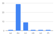
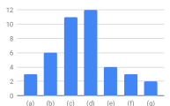
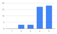
Below we include three questions from the survey discussed in Section 4 that measure participants’ interpretation of various terms or statistical tools. Next to each question, we show the distribution of the collected responses. In Q1 & Q2, reveal that individuals have substantial difficulties in interpreting $p-$values. In Q1, while (b) is the popular response, the correct answer is the much less popular option (c). In Q2, while (d) is the most popular response, the correct answer is (c).

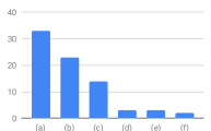
For Q3, as discussed in §4, researchers often find it difficult to interpret statements that contain “significant”. Therefore, we must be extra cautious about how this loaded keyword is used.

Q1: An NLP paper shows a performance of 38% for a classifier. They also show that adding a feature F improves the performance to 39%. In this finding, the authors have stated that $p$-value $>0.05$. This means:

1. The probability is greater than 1 in 20 that an improvement would be found again, if the study were repeated.

2. The probability is greater than 1 in 20 that an improvement this large could occur by chance alone.

3. The probability is less than 1 in 20 that an improvement this large could occur by chance alone.

4. The chance is 95% that the study is correct.

5. I don’t know, because I don’t know what $p$-value means.

6. Don’t have time. Skipping this question.

(a) Distribution of responses to Q1.

Q2: An NLP paper shows a performance of 38% for a classifier-1. They also show that adding a feature improves the performance to 45% (call this classifier-2). The authors claim that this finding is ”statistically significant” with a significance level of 0.01. Which of the following(s) make sense?

1. With probability at least 0.01 classifier-2 will have better results than classifier-1, if we repeat this experiment.

2. With probability 0.01 the observations are sampled from two equal classifiers.

3. The probability of observing a margin ≥ 7% is at most 0.01, assuming that the two classifiers inherently have the same performance.

4. If we repeat the experiment, with a probability 99% classifier-2 will have a higher performance than classifier-1.

5. If we repeat the experiment, with a probability 99% classifier-2 will have a performance margin of 7% compared to classifier-1.

6. I don’t know, because I don’t know how hypothesis testing is done.

7. Don’t have time. Skipping this question.

(a) Distribution of responses to Q2.

Q3: An NLP paper presents system-1 and it compares it with a baseline system-2. In its ”abstract” it writes: ” … system-1 significantly improves over system-2.” What are the right way(s) to interpret this (select all that applies)

1. It is expected that authors have performed some type of ”hypothesis testing.”

2. It is expected that the authors have reported the performances of two systems on a dataset where system-1 has a higher performance than system-2 with a notable margin in the dataset.

3. It is expected that the authors have reported experiments and concluded that system-1, inherently, has a higher perf. than system-2 with a notable margin.

4. It is expected that the authors conclude through theoretical arguments that, system-1 has a higher inherent perf. than system-2 with a notable margin.

5. Even though not expected, it is acceptable that the authors are concluding, through some theoretical arguments, that system-1 has a higher inherent performance than system-2 with a notable margin.

6. Too tedious. Skipping this question.

(a) Distribution of responses to Q3.

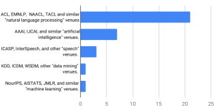
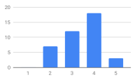
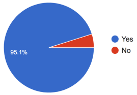
Responses to the remaining questions are summarized in Figure 9:

(a) Current positions of the participants in our survey.

(b) Distribution of responses to “What venues do you usually publish in?”

(c) Distribution of responses to “I have learned about statistical hypothesis testing/assessment (via taking classes or reading it from other places).”

(d) Distribution of responses to “I can understand almost all the ”statistical” terms I encounter in papers.”

(e) Distribution of responses to “Do you know the definition of Confidence Interval?”

(f) Distribution of responses to “I know $p$-values and I know how to interpret them.”

Figure 9: Responses to several questions in our survey of NLP researchers

Appendix C Comparison, Misinterpretations, and Fallacies

This is an extension of the ideas discussed in Section 3.

C.1 Susceptibility to Misinterpretation

The complexity of interpreting significance tests, combined with insufficient reporting (as shown by Dror et al. (2018)) could result in ambiguous or misleading conclusions. Not only many papers are unclear about their tests, but their results could also be misinterpreted by readers.

Among the techniques studied here, $p$-values, due to their complex definition, have received by far the biggest number of criticisms. While $p$-values are the most common approach, they are inherently complex which makes them easy to misinterpret. Here are a few common misinterpretations Demšar (2008); Goodman (2008):

• Misconception #1: If $p<0.05$, the null-hypothesis has only a 5% chance of being true: To see that this is false, remember that $p$-value is defined with the assumption that null-hypothesis is correct (Eq. 1.)

• Misconception #2: If $p>0.05$, there is no difference between the two systems: Having large $p$-value only means that the null-hypothesis is consistent with the observations, but it does not tell anything about the likeliness of the null-hypothesis.

• Misconception #3: A statistically significant result ($p<0.05$) indicates a large/notable difference between two systems: $p$-value only indicates strict superiority and provides no information about the margin of the effect.

Interpretation of CI can also be challenging since it is an extension of $p$-value Hoekstra et al. (2014). Tests that provide measures of uncertainty (like the ones in §2.3) are more natural choices for reporting the results of experiments Kruschke and Liddell (2018). Overall, our view on “ease of interpretation” of the approaches is summarized in Table 3.

C.2 Practical Significance

Statistical significance is different from practical significance Berger and Sellke (1987). While we saw in Example 1 that the difference between systems $S_{1}$ and $S_{2}$ is statistically significant (H1), it does not provide any intuition on the magnitude of their difference (the $x$ parameter in H2-4). In other words, a small $p$-value does not necessarily mean that the effect is practically important. Confidence intervals alleviate this issue by providing the range of parameters that are compatible with the data; however, they do not provide probability estimates Kruschke and Liddell (2018). Bayesian analysis provides probability distributions directly over the target parameters of interest. This allows users to report uncertainty estimates for hypotheses that capture the margins of the effects.

C.3 Unintended Misleading Result by Iterative Testing

While many tests are designed for a single-round experiment, in practice researchers perform multiple rounds of experiments until a predetermined condition is satisfied. This is particularly a problem in binary tests (such as $p$-value) when the condition is to achieve a desired result. For example, a researcher could continue experimenting until they achieve a statistically significant result (even if they don’t necessarily have any intention of cheating the test) Kim and Bang (2016).

Since the outcomes of $p$-values and CIs only can “reject” or stay “undecided”, these tests reinforce an unintentional bias towards the only possible decision. Consequently, it becomes easy to misuse this testing mechanism: for big enough data points it is possible to make statistically significant claims Amrhein et al. (2017).

On the other hand, the approaches in §2.3 and §2.4 provide both outcomes of “Accept” and “reject”, beside staying “undecided.” Therefore an honest researcher is more probable to accept that their data supports the opposite of what their conjecture was.

For an in-depth study of how each approach behaves in sequential tests, we refer to Kruschke (2010, §13.3).

Since $p$-values and CIs do not depend on prior they are not subject to this issue.

C.4 Choice of Prior for Bayes Factor

As discussed in §2.4, §C.3, and §5, Bayes Factor is quite sensitive to the choice of prior. To address this, here are a few options to set the prior:

1. Within the framework of model selection, if the priors are decided based on a clear meaning, as opposed to formulating a “vague” prior, then they can be justified to the audience.

2. Often, there are a few choices of non-committal priors that seem equally representative of our beliefs. The best option is to perform and report one test for each of these choices to control the sensitivity to the prior.

3. Another common approach to mitigate this concern is to use a small portion of the data to get an “informed” prior and do the analysis using this prior. This ensures that the new prior is meaningful and defensible.

4. If none the above applies, it is recommended to use the approaches in §2.3 instead. Even though posterior density depends on prior, this measure is known to be robust for different choices of similar priors.

C.5 Flexible Choice of Hierarchical Model

In this respect, the approaches in §2.3 and §2.4 are better suited to take the specifics of each setting into account.

C.6 Bayes Factors vs. Posterior Intervals

We refer interested readers to Kruschke and Liddell (2018, pp. 165-166) for a list of Bayes factor caveats.

References

- Amrhein et al. (2017) Valentin Amrhein, Fränzi Korner-Nievergelt, and Tobias Roth. 2017. The earth is flat (p 0.05): significance thresholds and the crisis of unreplicable research. PeerJ, 5:e3544.
- Berg-Kirkpatrick et al. (2012) Taylor Berg-Kirkpatrick, David Burkett, and Dan Klein. 2012. An empirical investigation of statistical significance in NLP. In Proceedings of EMNLP, pages 995–1005.
- Berger and Sellke (1987) James O Berger and Thomas Sellke. 1987. Testing a point null hypothesis: The irreconcilability of p values and evidence. Journal of the American Statistical Association, 82(397):112–122.
- Chinchor (1992) Nancy Chinchor. 1992. The statistical significance of the MUC-4 results. In Proceedings of the 4th conference on Message understanding, pages 30–50. Association for Computational Linguistics.
- Clark et al. (2018) Peter Clark, Isaac Cowhey, Oren Etzioni, Tushar Khot, Ashish Sabharwal, Carissa Schoenick, and Oyvind Tafjord. 2018. Think you have solved question answering? Try ARC, the AI2 Reasoning Challenge. CoRR, abs/1803.05457.
- Demšar (2008) Janez Demšar. 2008. On the appropriateness of statistical tests in machine learning. In Workshop on Evaluation Methods for Machine Learning in conjunction with ICML, page 65.
- Devlin et al. (2019) Jacob Devlin, Ming-Wei Chang, Kenton Lee, and Kristina Toutanova. 2019. BERT: Pre-training of deep bidirectional transformers for language understanding. In Proceedings of NAACL, pages 4171–4186.
- Dienes (2008) Zoltan Dienes. 2008. Understanding psychology as a science: An introduction to scientific and statistical inference. Macmillan International Higher Education.
- Dror et al. (2018) Rotem Dror, Gili Baumer, Segev Shlomov, and Roi Reichart. 2018. The hitchhiker’s guide to testing statistical significance in natural language processing. In Proceedings of ACL, pages 1383–1392.
- Dror and Reichart (2018) Rotem Dror and Roi Reichart. 2018. Recommended statistical significance tests for NLP tasks. arXiv preprint arXiv:1809.01448.
- Evert (2004) Stefan Evert. 2004. Significance tests for the evaluation of ranking methods. In Proceedings of COLING.
- Gamerman and Lopes (2006) Dani Gamerman and Hedibert F Lopes. 2006. Markov chain Monte Carlo: stochastic simulation for Bayesian inference. CRC Press.
- Gelman (2013) Andrew Gelman. 2013. The problem with p-values is how they’re used.
- Goodman (2008) Steven Goodman. 2008. A dirty dozen: Twelve p-value misconceptions. Seminars in Hematology, 45(3):135–140.
- Graham et al. (2014) Yvette Graham, Nitika Mathur, and Timothy Baldwin. 2014. Randomized significance tests in machine translation. In Proceedings of the Ninth Workshop on Statistical Machine Translation, pages 266–274.
- Hoekstra et al. (2014) Rink Hoekstra, Richard D Morey, Jeffrey N Rouder, and Eric-Jan Wagenmakers. 2014. Robust misinterpretation of confidence intervals. Psychonomic bulletin & review, 21(5):1157–1164.
- Kim and Bang (2016) Jeehyoung Kim and Heejung Bang. 2016. Three common misuses of p values. Dental hypotheses, 7(3):73.
- Koehn (2004) Philipp Koehn. 2004. Statistical significance tests for machine translation evaluation. In Proceedings of EMNLP.
- Kruschke (2010) John K Kruschke. 2010. Bayesian data analysis. Wiley Interdisciplinary Reviews: Cognitive Science, 1(5):658–676.
- Kruschke (2018) John K Kruschke. 2018. Rejecting or accepting parameter values in bayesian estimation. Advances in Methods and Practices in Psychological Science, 1(2):270–280.
- Kruschke and Liddell (2018) John K Kruschke and Torrin M Liddell. 2018. The bayesian new statistics: Hypothesis testing, estimation, meta-analysis, and power analysis from a bayesian perspective. Psychonomic Bulletin & Review, 25(1):178–206.
- Liu and Aitkin (2008) Charles C Liu and Murray Aitkin. 2008. Bayes factors: Prior sensitivity and model generalizability. Journal of Mathematical Psychology, 52(6):362–375.
- Metropolis et al. (1953) N. Metropolis, A.W. Rosenbluth, M.N. Rosenbluth, A.H. Teller, and E. Teller. 1953. Equation of state calculations by fast computing machines. The journal of chemical physics, 21:1087.
- Ojala and Garriga (2010) Markus Ojala and Gemma C Garriga. 2010. Permutation tests for studying classifier performance. JMLR, 11(Jun):1833–1863.
- Oliphant (2006) Travis E Oliphant. 2006. A Bayesian perspective on estimating mean, variance, and standard-deviation from data. Technical report, Brigham Young University. https://scholarsarchive.byu.edu/facpub/278/.
- du Prel et al. (2009) Jean-Baptist du Prel, Gerhard Hommel, Bernd Röhrig, and Maria Blettner. 2009. Confidence interval or p-value?: Part 4 of a series on evaluation of scientific publications. Deutsches Ärzteblatt International, 106(19):335.
- Riezler and Maxwell (2005) Stefan Riezler and John T Maxwell. 2005. On some pitfalls in automatic evaluation and significance testing for mt. In Proceedings of the ACL workshop on intrinsic and extrinsic evaluation measures for machine translation and/or summarization, pages 57–64.
- Sinharay and Stern (2002) Sandip Sinharay and Hal S Stern. 2002. On the sensitivity of Bayes factors to the prior distributions. The American Statistician, 56(3):196–201.
- Søgaard et al. (2014) Anders Søgaard, Anders Johannsen, Barbara Plank, Dirk Hovy, and Héctor Martínez Alonso. 2014. What’s in a p-value in NLP? In Proceedings of CoNLL, pages 1–10.
- Sun et al. (2018) Kai Sun, Dian Yu, Dong Yu, and Claire Cardie. 2018. Improving machine reading comprehension with general reading strategies. In Proceedings of NAACL.
- Trafimow and Marks (2015) David Trafimow and Michael Marks. 2015. Editorial. Basic and Applied Social Psychology, 37(1):1–2.
- Wasserstein et al. (2016) Ronald L Wasserstein, Nicole A Lazar, et al. 2016. The ASA’s statement on p-values: context, process, and purpose. The American Statistician, 70(2):129–133.
- Windish et al. (2007) Donna M Windish, Stephen J Huot, and Michael L Green. 2007. Medicine residents’ understanding of the biostatistics and results in the medical literature. Jama, 298(9):1010–1022.