High-order accurate entropy stable nodal discontinuous Galerkin schemes for the ideal special relativistic magnetohydrodynamics

Abstract

This paper studies high-order accurate entropy stable nodal discontinuous Galerkin (DG) schemes for the ideal special relativistic magnetohydrodynamics (RMHD). It is built on the modified RMHD equations with a particular source term, which is analogous to the Powell’s eight-wave formulation and can be symmetrized so that an “entropy pair” is obtained. We design an affordable “fully consistent” two-point entropy conservative flux, which is not only consistent with the physical flux, but also maintains the zero parallel magnetic component, and then construct high-order accurate semi-discrete entropy stable DG schemes based on the quadrature rules and the entropy conservative and stable fluxes. They satisfy the semi-discrete “entropy inequality” for the given “entropy pair” and are integrated in time by using the high-order explicit strong stability preserving Runge-Kutta schemes to get further the fully-discrete nodal DG schemes. Extensive numerical tests are conducted to validate the accuracy and the ability to capture discontinuities of our schemes. Moreover, our entropy conservative flux is compared to an existing flux through some numerical tests. The results show that the zero parallel magnetic component in the numerical flux can help to decrease the error in the parallel magnetic component in one-dimensional tests, but two entropy conservative fluxes give similar results since the error in the magnetic field divergence seems dominated in the two-dimensional tests.

1 Introduction

This paper is concerned with the high-order accurate numerical schemes for the ideal special relativistic magnetohydrodynamic (RMHD) equations. In the covariant form, the four-dimensional space-time RMHD equations can be written as follows [1]

$$\nabla_{\alpha}(\rho u^{\alpha})=0,\ \ \nabla_{\alpha}\mathrm{T}^{\alpha\beta}=0,\ \ \nabla_{\alpha}\Psi^{\alpha\beta}=0,$$ (1.1)

where the Einstein summation convention has been used, $\rho$ and $u^{\alpha}$ denote the rest-mass density and the four-velocity vector, respectively, $\nabla_{\alpha}$ denotes the covariant derivative with respect to the four-dimensional space-time coordinates $(t,x^{1},x^{2},x^{3})$, the Greek indices run from $0$ to $3$ (or $t,x,y,z$),

$$\Psi^{\alpha\beta}=u^{\alpha}b^{\beta}-u^{\beta}b^{\alpha},$$ (1.2)

and $\mathrm{T}^{\alpha\beta}$ is the energy-momentum tensor and can be decomposed into the fluid part $\mathrm{T}^{\alpha\beta}_{f}$ and the electromagnetic part $\mathrm{T}^{\alpha\beta}_{m}$, defined by

$$\mathrm{T}^{\alpha\beta}_{f} =(e+p)u^{\alpha}u^{\beta}+pg^{\alpha\beta},$$ (1.3)

$$\mathrm{T}^{\alpha\beta}_{m} =\lvert b\rvert^{2}(u^{\alpha}u^{\beta}+g^{\alpha\beta}/2)-b^{\alpha}b^{\beta}.$$ (1.4)

Here $b^{\alpha}$ and $e$ are the covariant magnetic field and the total energy density, respectively.

Throughout this paper, the metric tensor $g^{\alpha\beta}$ is taken as the Minkowski tensor, i.e. $g^{\alpha\beta}=\mathrm{diag}\{-1,1,1,1\}$, and units in which the speed of light is equal to one will be used. The relations between the four-vectors $u^{\alpha}$ and $b^{\alpha}$, and the spatial components of the velocity $\bm{v}=(v_{1},v_{2},v_{3})$ and the laboratory magnetic field $\bm{B}=(B_{1},B_{2},B_{3})$ are

$$u^{\alpha}=W(1,\bm{v}),$$ (1.5)

$$b^{\alpha}=W\left(\bm{v}\cdot\bm{B},\frac{\bm{B}}{W^{2}}+\bm{v}(\bm{v}\cdot\bm{B})\right),$$ (1.6)

with

$$u^{\alpha}u_{\alpha}=-1,\quad u^{\alpha}b_{\alpha}=0,\quad\lvert b\rvert^{2}\equiv b^{\alpha}b_{\alpha}=\frac{\lvert\bm{B}\rvert^{2}}{W^{2}}+(\bm{v}\cdot\bm{B})^{2},$$ (1.7)

where $W=1/\sqrt{1-\lvert\bm{v}\rvert^{2}}$ is the Lorentz factor. To close the system (1.1)-(1.4), this paper considers the equation of state (EOS) for the perfect gas

$$p=(\Gamma-1)\rho\epsilon,$$

with the adiabatic index $\Gamma\in(1,2]$, where $\epsilon=e/\rho-1$ is the specific internal energy.

For the computational purpose, the system (1.1)-(1.4) should be rewritten in a lab frame as follows

$$\dfrac{\partial{\bm{U}}}{\partial{t}}+\sum_{k}\dfrac{\partial{\bm{F}_{k}(\bm{U})}}{\partial{x^{k}}}=0,$$ (1.8)

with the divergence-free constraint on the magnetic field

$$\sum_{k}\dfrac{\partial{B_{k}}}{\partial{x^{k}}}=0,$$ (1.9)

where $\bm{U}$ and $\bm{F}_{k}$ are respectively the conservative variables vector and the flux vector along the $x^{k}$-direction, and defined by

$$\begin{aligned} &\bm{U}=(D,\bm{m},E,\bm{B})^{\mathrm{T}},\\ &\bm{F}_{k}=(Dv_{k},\bm{m}v_{k}-B_{k}(\bm{B}/W^{2}+(\bm{v}\cdot\bm{B})\bm{v})+p_{\text{tot}}\bm{e}_{k},m_{k},v_{k}\bm{B}-B_{k}\bm{v})^{\mathrm{T}},\end{aligned}$$ (1.10)

with the mass density $D=\rho W$, the momentum density $\bm{m}=(\rho hW^{2}+\lvert\bm{B}\rvert^{2})\bm{v}-(\bm{v}\cdot\bm{B})\bm{B}$, the energy density $E=DhW-p_{\text{tot}}+\lvert\bm{B}\rvert^{2}$, and $\bm{e}_{k}$ denotes the $k$-th row of the $3\times 3$ unit matrix. Here, $p_{\text{tot}}$ denotes the total pressure containing the gas pressure $p$ and the magnetic pressure $p_{m}=\frac{1}{2}\lvert b\rvert^{2}$, and $h$ is the specific enthalpy defined by $h=(e+p)/\rho$. Because there is no explicit expression for the primitive variables $(\rho,\bm{v},p,\bm{B})^{\mathrm{T}}$ and the flux $\bm{F}_{k}$ in terms of $\bm{U}$, a nonlinear algebraic equation should be solved (the approach [37] is used by us), in order to recover the values of the primitive variables and the flux from the given $\bm{U}$.

The RMHD system (1.1)-(1.4) considers the relativistic description for the dynamics of the fluid (gas) at nearly the speed of light when the astrophysical phenomena are investigated from stellar to galactic scales, e.g. coalescing neutron stars, core collapse supernovae, active galactic nuclei, superluminal jets, the formation of black holes, and gamma-ray bursts, etc. It is obvious that its nonlinearity becomes much stronger than the non-relativistic case because of the relativistic effect, thus it is very difficult and challenging to treat it analytically. Numerical simulation is a useful way leading us to a better understanding of the physical mechanisms in the relativistic hydrodynamics (RHD) and the RMHDs. The first numerical work may date back to the artificial viscosity method for the RHD equations in the Lagrangian coordinates [47, 48] and the Eulerian coordinates [64]. Since the early 1990s, the modern shock-capturing methods were extended to the RHDs and RMHDs, such as the Roe-type scheme [2, 22], the Harten-Lax-van Leer (HLL) method [16, 17, 53, 60], the Harten-Lax-van Leer Contact (HLLC) method [42, 50, 51], the essentially non-oscillatory (ENO) and the weighted ENO (WENO) methods [20, 16, 17], the piecewise parabolic methods [44, 52], the Runge-Kutta discontinuous Galerkin (DG) methods with WENO limiter [80, 81], the direct Eulerian generalized Riemann problem schemes [70, 75, 76, 77], the two-stage fourth-order time discretization [78], the adaptive moving mesh methods [31, 32], and so on. The readers are referred to the early review articles [27, 45, 46] for more references. Recently, the properties of the admissible state set and the physical-constraints-preserving (PCP) numerical schemes were well studied for the RHDs and RMHDs, see [66, 71, 72, 73, 74]. For the numerical solutions of the RMHD equations, we need to deal carefully with the divergence-free constraint (1.9). In the non-relativistic case, many works have focused on this issue, for example, the projection method [9], the constrained transport (CT) method [23], the eight-wave formulation of the MHD equations [58], the hyperbolic divergence cleaning method [15], the locally divergence-free DG method [40], the “exactly” divergence-free central DG method [41]. Some of those works have been extended to the relativistic case, such as [5, 17, 55, 81].

For the RMHD equations, the entropy condition is an important property which must be satisfied according to the second law of thermodynamics. On the other hand, it is well known that the weak solution of the quasi-linear hyperbolic conservation laws might not be unique so that the entropy condition is needed to single out the unique physical relevant solution among all the weak solutions. Thus it is a matter of cardinal significance to seek the entropy stable schemes (satisfying some discrete or semi-discrete entropy conditions) for the quasi-linear system of hyperbolic conservation laws.

Definition 1.1.

A strictly convex scalar function $\eta(\bm{U})$ is called an entropy function for the system (1.8)-(1.10) if there are associated entropy fluxes $q_{k}(\bm{U})$ such that

$$q_{k}^{\prime}(\bm{U})=\bm{V}^{\mathrm{T}}\bm{F}_{k}^{\prime}(\bm{U}),$$ (1.11)

where $\bm{V}=\eta^{\prime}(\bm{U})^{\mathrm{T}}$ is called the entropy variables, and $(\eta,q_{k})$ is an entropy pair.

For the smooth solutions of (1.8)-(1.10), multiplying (1.8) by $\bm{V}^{\mathrm{T}}$ gives the entropy identity

$$\dfrac{\partial{\eta(\bm{U})}}{\partial{t}}+\sum_{k}\dfrac{\partial{q_{k}(\bm{U})}}{\partial{x^{k}}}=0.$$

However, if the solution contains a discontinuity, then the above identity does not hold.

Definition 1.2.

A weak solution $\bm{U}$ of (1.8)-(1.10) is called an entropy solution if for all entropy functions $\eta$, the inequality

$$\dfrac{\partial{\eta(\bm{U})}}{\partial{t}}+\sum_{k}\dfrac{\partial{q_{k}(\bm{U})}}{\partial{x^{k}}}\leqslant 0,$$ (1.12)

holds in the sense of distributions.

For the scalar conservation laws, the conservative monotone schemes were nonlinearly stable and satisfied the discrete entropy conditions, thus they could converge to the entropy solution [14, 30]. A class of so-called E-schemes satisfying the entropy condition for any convex entropy was studied in [56, 57], but they were only first-order accurate. Generally, it is hard to show that the high-order schemes of the scalar conservation laws and the schemes for the system of hyperbolic conservation laws satisfy the entropy inequality for any convex entropy function. Two relative works were presented in [8] and [34]. The former is second-order accurate and not in the standard finite volume form, while the latter approximates the entropy variables and needs solving nonlinear equations at each time step. A lot of people are trying to study the high-order accurate entropy stable schemes, which satisfy the entropy inequality for a given entropy pair. The second-order entropy conservative schemes (satisfying the discrete entropy identity) were studied in [61, 62], and their higher-order extension was considered in [39]. It is known that the entropy conservative schemes may become oscillatory near the shock waves so that some additional dissipation term has to be added to obtain the entropy stable schemes (satisfying the discrete entropy inequality). Combining the entropy conservative flux with the “sign” property of the ENO reconstruction, the arbitrary high-order entropy stable schemes were constructed by using high-order dissipation terms [25]. The entropy stable schemes based on summation-by-parts (SBP) operators were developed for the Navier-Stokes equations [24]. The semi-discrete DG schemes for scalar conservation laws were proved to satisfy a discrete entropy inequality for the square entropy [36], and some entropy stable DG schemes were also studied, such as the space-time DG formulation [4, 33] and the entropy stable nodal DG schemes using suitable quadrature rules for the conservation laws [12] and the MHD equations [43]. As a base of those works, constructing the affordable two-point entropy conservative flux is very important, and has been extended to the shallow water equations [28], the RHD equations [21], the MHD equations [11, 65, 18], very recently the RMHD equations [69], and so on. Because it can be verified that the original MHD equations cannot be symmetrized, which is also true for the RMHD equations, most of the above mentioned MHD works are based on the modified MHD equations with a non-conservative source term, which is first introduced by Godunov [29] in one-dimensional case, and then extended to multi-dimensional cases by Powell [58]. Due to introducing the source term, the sufficient condition proposed in [61] for a finite difference or volume scheme to satisfy an entropy identity should be modified, see [11, 65], and in the DG framework, the non-conservative source term should also be carefully discretized [43].

This paper aims at studying the high-order accurate entropy stable nodal DG schemes for the RMHD equations. Because the conservative RMHD equations cannot be symmetrized, a suitable non-conservative source term should be added to obtain the modified RMHD equations, which can be symmetrized by the entropy pair following [29]. By using the modified RMHD equations and suitable quadrature rules as well as the SBP, high-order accurate entropy stable DG schemes satisfying the entropy inequality for the given entropy pair are constructed, where the so-called two-point entropy conservative flux is used in the integral over the cell, while the entropy stable fluxes are used at the cell interfaces, e.g., the Godunov flux, the HLL flux with suitably chosen wave speeds, the Lax-Friedrichs flux, and so on. It can be shown that the temporal change of the total entropy in each cell for such semi-discrete scheme is only effected from the entropy stable fluxes at the cell interfaces. One of our main tasks is to technically design the affordable two-point entropy conservative flux with zero parallel magnetic component, which is “fully consistent” with the physical flux (Note that the parallel magnetic component of the physical flux is always zero). It is worth noting that in a very recent and independent work [69], an entropy conservative scheme is constructed with a suitable discretization of the source term, but its parallel magnetic component of the entropy conservative flux does not always vanish. This paper will give a comparison of those entropy conservative fluxes by some numerical tests to validate that our newly derived entropy conservative flux may serve as a better base of the entropy conservative or stable schemes for the RMHD equations.

The paper is organized as follows. Section 2 introduces the modified symmetrizable RMHD equations. Section 3 presents the 1D entropy stable nodal DG schemes and constructs the affordable two-point entropy conservative flux for the one-dimensional RMHD equations. Section 4 extends the results to the two-dimensional cases. Extensive numerical tests are conducted in Section 5 to validate the effectiveness of our schemes. Section 6 gives some conclusions.

2 Symmetrization of the ideal special RMHD equations

This section gives a derivation of the symmetrizable RMHD equations, which is analogous to the non-relativistic case. First of all, we want to show that the RMHD equations (1.8)-(1.10) are not symmetrizable by using the entropy pair based on the thermodynamical entropy as in the RHD case [21]. For the smooth solutions of the special RMHD equations (1.8)-(1.10), if defining the thermodynamical entropy

$$s=\ln(p)-\Gamma\ln(\rho),$$

then from (1.8)-(1.10) and the first law of thermodynamics

$$T~{}\mathrm{d}s=\mathrm{d}(e/\rho)+p\mathrm{d}(1/\rho),$$

one can show [1] that

$$\dfrac{\partial{s}}{\partial{t}}+\sum_{k}v_{k}\dfrac{\partial{s}}{\partial{x^{k}}}+\frac{(\bm{v}\cdot\bm{B})\nabla\cdot{\bm{B}}}{\rho\epsilon}=0,$$

where $T$ is the temperature, which is equal to $\epsilon$ under the assumptions in this paper. Combining it with the first equation in (1.8) obtains

$$\dfrac{\partial{(\rho Ws)}}{\partial{t}}+\sum_{k}\dfrac{\partial{(\rho v_{k}Ws)}}{\partial{x^{k}}}+\frac{(\Gamma-1)\rho W(\bm{v}\cdot\bm{B})\nabla\cdot{\bm{B}}}{p}=0,$$ (2.1)

which implies that the following quantities

$${\eta}(\bm{U})=\dfrac{-\rho Ws}{\Gamma-1},\quad{q_{k}}(\bm{U})=\dfrac{-\rho v_{k}Ws}{\Gamma-1},$$ (2.2)

satisfy an additional conservation law

$$\dfrac{\partial{\eta}}{\partial{t}}+\sum_{k}\dfrac{\partial{q_{k}}}{\partial{x^{k}}}=0,$$ (2.3)

under the constraint $\nabla\cdot{\bm{B}}=0$. However, unfortunately, the pair $(\eta,q_{k})$ defined in (2.2) does not satisfy (1.11), since

$$q_{k}^{\prime}(\bm{U})=\bm{V}^{\mathrm{T}}\bm{F}_{k}^{\prime}(\bm{U})+\dfrac{\rho W}{p}(\bm{v}\cdot\bm{B})B_{k}^{\prime}(\bm{U}),$$ (2.4)

where the vector $\bm{V}={\eta}^{\prime}(\bm{U})^{\mathrm{T}}$ is explicitly given by

$$\bm{V}=(V_{1},\cdots,V_{8})^{\mathrm{T}}=\left(\dfrac{\Gamma-s}{\Gamma-1}+\dfrac{\rho}{p},\dfrac{\rho u^{x}}{p},\dfrac{\rho u^{y}}{p},\dfrac{\rho u^{z}}{p},-\dfrac{\rho W}{p},\dfrac{\rho b^{x}}{p},\dfrac{\rho b^{y}}{p},\dfrac{\rho b^{z}}{p}\right)^{\mathrm{T}}.$$

Moreover, the pair $(\eta,q_{k})$ cannot symmetrize the RMHD system (1.8)-(1.10), because it can be verified that the matrix $\dfrac{\partial{\bm{U}}}{\partial{\bm{V}}}$ is symmetric and positive definite, but $\dfrac{\partial{\bm{F}_{k}}}{\partial{\bm{V}}}$ is not symmetric.

To derive a symmetrizable RMHD system for (1.8)-(1.10), one needs to add some non-conservative source terms, similar to those for the non-relativistic ideal MHD equations [29, 58], to get a modified RMHD system as follows

$$\dfrac{\partial{\bm{U}}}{\partial{t}}+\dfrac{\partial{\bm{F}_{k}}}{\partial{x^{k}}}+\Phi^{\prime}(\bm{V})^{\mathrm{T}}\nabla\cdot{\bm{B}}=0,$$ (2.5)

where $\Phi(\bm{V})$ is a homogeneous function of degree one, i.e. $\Phi=\Phi^{\prime}(\bm{V})\bm{V}$. Taking the dot product of $\bm{V}=\eta^{\prime}(\bm{U})^{\mathrm{T}}$ with (2.5) yields

$$\bm{V}^{\mathrm{T}}\dfrac{\partial{\bm{U}}}{\partial{t}} +\left(\bm{V}^{\mathrm{T}}\dfrac{\partial{\bm{F}_{k}}}{\partial{\bm{U}}}+\Phi(\bm{V})\dfrac{\partial{B_{k}}}{\partial{\bm{U}}}\right)\dfrac{\partial{\bm{U}}}{\partial{x^{k}}}$$

$$= \dfrac{\partial{\eta}}{\partial{t}}+\left(\dfrac{\partial{q_{k}}}{\partial{\bm{U}}}+\left(\Phi(\bm{V})-\dfrac{\rho W}{p}(\bm{v}\cdot\bm{B})\right)\dfrac{\partial{B_{k}}}{\partial{\bm{U}}}\right)\dfrac{\partial{\bm{U}}}{\partial{x^{k}}}=0.$$

It is obvious that the above equation becomes the identity (2.3) if defining the homogeneous function $\Phi$ by

$$\Phi(\bm{V})=\dfrac{\rho W(\bm{v}\cdot\bm{B})}{p}=-\dfrac{V_{2}V_{6}+V_{3}V_{7}+V_{4}V_{8}}{V_{5}}.$$

One can verify that $\Phi^{\prime}(\bm{V})=\big{(}0,\dfrac{b^{x}}{W},\dfrac{b^{y}}{W},\dfrac{b^{z}}{W},\bm{v}\cdot\bm{B},\bm{v}\big{)}$ and the pair $(\eta,q_{k})$ can symmetrize the modified RMHD system (2.5) because applying the change of variables $\bm{V}=\bm{V}(\bm{U})$ gives

$$\dfrac{\partial{\bm{U}}}{\partial{\bm{V}}}\dfrac{\partial{\bm{V}}}{\partial{t}}+\left(\dfrac{\partial{\bm{F}_{k}}}{\partial{\bm{V}}}+\Phi^{\prime}(\bm{V})\dfrac{\partial{B_{k}}}{\partial{\bm{V}}}\right)\dfrac{\partial{\bm{V}}}{\partial{x^{k}}}=0,$$

and $\dfrac{\partial{\bm{F}_{k}}}{\partial{\bm{V}}}+\Phi^{\prime}(\bm{V})\dfrac{\partial{B_{k}}}{\partial{\bm{V}}}$ is symmetric. Notice that the identity (2.3) is obtained without using the divergence-free condition, and useful in constructing an entropy stable scheme because the numerical divergence may not be zero. Moreover, we can define the “entropy potential” $\psi_{k}$ from given $(\eta(\bm{U}),q_{k}(\bm{U}))$ by

$$\psi_{k}:=\bm{V}^{\mathrm{T}}\bm{F}_{k}(\bm{U})+\Phi(\bm{V})B_{k}-q_{k}(\bm{U})=\rho v_{k}W+\dfrac{\rho v_{k}W\lvert b\rvert^{2}}{2p},$$ (2.6)

which makes the following identity true

$$\int_{\Omega}\left(\dfrac{\partial{\eta}}{\partial{t}}+\dfrac{\partial{q_{k}}}{\partial{x^{k}}}\right)\mathrm{d}\bm{x}= \int_{\Omega}\bm{V}^{\mathrm{T}}\left(\dfrac{\partial{\bm{U}}}{\partial{t}}+\dfrac{\partial{\bm{F}_{k}(\bm{U})}}{\partial{x^{k}}}+\Phi^{\prime}(\bm{V})^{\mathrm{T}}\nabla\cdot{\bm{B}}\right)\mathrm{d}\bm{x}$$

$$= \int_{\Omega}\left(\dfrac{\partial{\eta(\bm{U})}}{\partial{t}}+\dfrac{\partial{(\bm{V}^{\mathrm{T}}\bm{F}_{k}(\bm{U}))}}{\partial{x^{k}}}-\dfrac{\partial{\bm{V}^{\mathrm{T}}}}{\partial{x^{k}}}\bm{F}(\bm{U})+\Phi(\bm{V})\nabla\cdot{\bm{B}}\right)\mathrm{d}\bm{x}$$

$$= \int_{\Omega}\left(\dfrac{\partial{\eta(\bm{U})}}{\partial{t}}+\dfrac{\partial{(\bm{V}^{\mathrm{T}}\bm{F}_{k}(\bm{U}))}}{\partial{x^{k}}}-\dfrac{\partial{\psi_{k}(\bm{U})}}{\partial{x^{k}}}+\Phi(\bm{V})\nabla\cdot{\bm{B}}\right)\mathrm{d}\bm{x}.$$

The “entropy potential” plays an important role in obtaining the sufficient condition for the two-point entropy conservative fluxes.

Remark 2.1.

Combining the modified induction equations and the first equation in (1.8) gives

$$\dfrac{\partial}{\partial t}\left(\dfrac{\nabla\cdot{\bm{B}}}{\rho W}\right)+\bm{v}\cdot\nabla\left(\dfrac{\nabla\cdot{\bm{B}}}{\rho W}\right)=0,$$

which implies that the errors in divergence may be transported by the flow. However, one drawback is that the non-conservative source term may lead to incorrect solutions.

3 One-dimensional entropy stable DG schemes

This section considers the one-dimensional $x$-splitting system of (2.5), i.e.,

$$\dfrac{\partial{\bm{U}}}{\partial{t}}+\dfrac{\partial{\bm{F}_{1}(\bm{U})}}{\partial{x}}=-\Phi^{\prime}(\bm{V})^{\mathrm{T}}\dfrac{\partial{B_{1}}}{\partial{x}}.$$ (3.1)

3.1 Spatial DG discretization

Assume that the computational domain $\Omega$ is divided into $N_{x}$ cells, $I_{i}=(x_{{i-\frac{1}{2}}},x_{{i+\frac{1}{2}}})$, $i=1,2,\cdots,N_{x}$, where $x_{\frac{1}{2}}<x_{\frac{3}{2}}<\dots<x_{N_{x}+\frac{1}{2}}$. Denote the center of $I_{i}$ and the mesh size by $x_{i}=\frac{1}{2}(x_{{i-\frac{1}{2}}}+x_{{i+\frac{1}{2}}})$ and $\Delta x_{i}=x_{{i+\frac{1}{2}}}-x_{{i-\frac{1}{2}}}$ respectively. The spatial DG approximation space is

$$\bm{W}^{r}_{h}=\{\bm{w}_{h}\in\left[L^{2}(\Omega)\right]^{8}:~{}\bm{w}_{h}|_{I_{i}}\in[P^{r}(I_{i})]^{8},i=1,2,\dots,N_{x}\},$$ (3.2)

where $P^{r}(I_{i})$ denotes all polynomials of degree at most $r$ on $I_{i}$. Let us multiply (3.1) with the test function $\bm{w}_{h}\in\bm{W}^{r}_{h}$, integrating it over the control volume $I_{i}$, and introducing the numerical fluxes at the cell interfaces following [43], then the spatial DG approximation for (3.1) is to find $\bm{U}_{h}\in\bm{W}^{r}_{h}$, satisfying

$$\frac{d}{dt}\int_{I_{i}}\bm{U}_{h}^{\mathrm{T}}\bm{w}_{h}\mathrm{d}x= \int_{I_{i}}\bm{F}_{1}(\bm{U}_{h})^{\mathrm{T}}\dfrac{\partial{\bm{w}_{h}}}{\partial{x}}\mathrm{d}x-\int_{I_{i}}\Phi^{\prime}(\bm{U}_{h})\dfrac{\partial{(B_{1})_{h}}}{\partial{x}}\bm{w}_{h}\mathrm{d}x$$

$$-\hat{\bm{F}}_{i+\frac{1}{2}}^{\mathrm{T}}\bm{w}_{h}(x_{i+\frac{1}{2}}^{-})+\hat{\bm{F}}_{i-\frac{1}{2}}^{\mathrm{T}}\bm{w}_{h}(x_{i-\frac{1}{2}}^{+})$$

$$-\frac{1}{2}\Phi^{\prime}(\bm{U}_{h}(x_{i+\frac{1}{2}}^{-}))\llbracket(B_{1})_{h}\rrbracket_{i+\frac{1}{2}}\bm{w}_{h}(x_{i+\frac{1}{2}}^{-})$$

$$-\frac{1}{2}\Phi^{\prime}(\bm{U}_{h}(x_{i-\frac{1}{2}}^{+}))\llbracket(B_{1})_{h}\rrbracket_{i-\frac{1}{2}}\bm{w}_{h}(x_{i-\frac{1}{2}}^{+}),$$ (3.3)

for any $\bm{w}_{h}\in\bm{W}^{r}_{h}$ and $i=1,2,\cdots,N_{x}$, where $\llbracket(B_{1})_{h}\rrbracket=(B_{1})_{h}^{+}-(B_{1})_{h}^{-}$ denotes the jump of $(B_{1})_{h}$ at the cell interface, with the superscripts $+,-$ denoting its right and left limits, and $\hat{\bm{F}}_{i+\frac{1}{2}}$ is a two-point numerical flux

$$\hat{\bm{F}}_{i+\frac{1}{2}}=\hat{\bm{F}}(\bm{U}_{h}(x_{i+\frac{1}{2}}^{-}),\bm{U}_{h}(x_{i+\frac{1}{2}}^{+})),$$ (3.4)

which is consistent with the physical flux $\bm{F}_{1}$ in (3.1). Notice that the discretization of the non-conservative source term is originally proposed for directly solving the Hamilton-Jacobi equations [13].

In what follows, the derivation of the entropy conservative and stable DG schemes largely relies on the summation-by-parts (SBP) operator. The key idea is to approximate the integrals in (3.1) by using the $(r+1)$-point Legendre-Gauss-Lobatto quadrature rule. For the reference element $I=[-1,1]$, denote the Legendre-Gauss-Lobatto quadrature points as

$$-1=\xi_{0}<\xi_{1}<\cdots<\xi_{r}=1,$$

and corresponding weights as $\omega_{j},j=0,1,\cdots,r$. Define the Lagrangian basis polynomials by

$$L_{j}(\xi)=\prod\limits_{l=0,l\not=j}^{r}\dfrac{\xi-\xi_{l}}{\xi_{j}-\xi_{l}},\ j=0,1,\cdots,r,$$

the difference matrix $\bm{D}=({D}_{jl})$ and the mass matrix $\bm{M}=({M}_{jl})$ respectively by

$${D}_{jl}=L_{l}^{\prime}(\xi_{j}),\ \ {M}_{jl}=\langle{L_{j}},{L_{l}}\rangle_{\omega}=\omega_{j}\delta_{jl},$$

where

$$\langle{u},{v}\rangle_{\omega}=\sum_{j=0}^{r}\omega_{j}u(\xi_{j})v(\xi_{j}).$$

It is obvious that $L_{j}(\xi_{l})=\delta_{jl}$, $\bm{M}=\text{diag}\{\omega_{0},\cdots,\omega_{r}\}$, and the matrices $\bm{M}$ and $\bm{D}$ satisfy the following property.

Proposition 3.1.

The identity for the matrices $\bm{M}$ and $\bm{D}$

$$\bm{M}\bm{D}+\bm{D}^{\mathrm{T}}\bm{M}=\bm{B},\$$ (3.5)

holds, where $\bm{B}$ is the boundary matrix defined by

$$\bm{B}=\text{diag}\{-1,0,\cdots,0,1\}=:\text{diag}\{\tau_{0},\cdots,\tau_{r}\}.$$

The above property is usually considered as the summation-by-parts (SBP) property, which is a discrete analog of the integration by parts, that is, $\bm{\xi}^{T}\bm{M}\bm{D}\bm{\eta}+\bm{\xi}^{T}\bm{D}^{\mathrm{T}}\bm{M}\bm{\eta}=\bm{\xi}^{T}\bm{B}\bm{\eta}$, $\bm{\xi},\bm{\eta}\in\mathbb{R}^{r+1}$.

Now the integrals in (3.1) can be approximated by using the $(r+1)$-point Legendre-Gauss-Lobatto quadrature rule and the SBP property (3.5) to derive the semi-discrete nodal DG scheme as follows

$$\dfrac{\mathrm{d}\bm{U}_{i}^{l}}{\mathrm{d}t}= -\dfrac{4}{\Delta x_{i}}\sum_{p=0}^{r}{D}_{lp}{\tilde{\bm{F}}_{1}(\bm{U}_{i}^{p},\bm{U}_{i}^{l})}-\dfrac{2}{\Delta x_{i}}\sum_{p=0}^{r}{D}_{lp}(\Phi_{i}^{{}^{\prime}l})^{\mathrm{T}}(B_{1})_{i}^{p}$$

$$+\dfrac{2}{\Delta x_{i}}\dfrac{\tau_{l}}{\omega_{l}}\left(\bm{F}_{i,1}^{l}-\bm{F}_{i,1,*}^{l}\right)+\dfrac{2}{\Delta x_{i}}\dfrac{\tau_{l}}{\omega_{l}}\bm{s}_{i}^{l},\ l=0,\cdots,r,$$ (3.6)

where the transformation between $I_{i}$ and $I$ is $x_{i}(\xi)=\frac{1}{2}(x_{i-\frac{1}{2}}+x_{i+\frac{1}{2}})+\frac{\xi}{2}\Delta x_{i}$, and

$$\bm{U}_{i}^{l}=\bm{U}_{h}(x_{i}(\xi_{l})),\quad\bm{F}_{i,1}^{l}=\bm{F}_{1}(\bm{U}_{i}^{l}),\quad(\Phi_{i}^{{}^{\prime}l})^{\mathrm{T}}=\Phi^{\prime}(\bm{V}(\bm{U}_{i}^{l}))^{\mathrm{T}},\quad l=0,1,\cdots,r,$$

$$\vec{\bm{F}}_{i,1,*}=\begin{bmatrix}\bm{F}_{i,1,*}^{0},\bm{F}_{i,1,*}^{1},\cdots,\bm{F}_{i,1,*}^{r}\end{bmatrix}:=\begin{bmatrix}\hat{\bm{F}}_{i-\frac{1}{2}}(\bm{U}_{i-1}^{r},\bm{U}_{i}^{0}),0,\cdots,0,\hat{\bm{F}}_{i+\frac{1}{2}}(\bm{U}_{i}^{r},\bm{U}_{i+1}^{0})\end{bmatrix},$$

$$\vec{\bm{s}}_{i}=\begin{bmatrix}\bm{s}_{i}^{0},\bm{s}_{i}^{1},\cdots,\bm{s}_{i}^{r}\end{bmatrix}:=\begin{bmatrix}\dfrac{1}{2}(\Phi_{i}^{{}^{\prime}0})^{\mathrm{T}}[(B_{1})_{i}^{0}-(B_{1})_{i-1}^{r}],0,&\cdots,0,-\dfrac{1}{2}(\Phi_{i}^{{}^{\prime}r})^{\mathrm{T}}[(B_{1})_{i+1}^{0}-(B_{1})_{i}^{r}]\end{bmatrix}.$$

The numerical fluxes $\tilde{\bm{F}}_{1}(\bm{U}_{i}^{p},\bm{U}_{i}^{l})$, $l,p=0,1,\cdots,r$, are further used to approximate the fluxes in the volume integrals in (3.1), respectively. The purpose of this work is to develop the entropy stable DG scheme, that is, to derive the two-point entropy conservative flux $\bm{F}_{1}^{EC}(\bm{U}_{i}^{p},\bm{U}_{i}^{l})$, and use $\bm{F}_{1}^{EC}(\bm{U}_{i}^{p},\bm{U}_{i}^{l})$ and the entropy stable flux $\hat{\bm{F}}^{ES}_{i\pm\frac{1}{2}}$ to replace respectively $\tilde{\bm{F}}_{1}(\bm{U}_{i}^{p},\bm{U}_{i}^{l})$ and $\hat{\bm{F}}_{i\pm\frac{1}{2}}$ in (3.6).

Definition 3.1.

For a given entropy pair, if a consistent, symmetric two-point numerical flux $\tilde{\bm{F}}_{1}(\bm{U}_{L},\bm{U}_{R})$ satisfies

$$\llbracket\bm{V}\rrbracket^{\mathrm{T}}\cdot{\tilde{\bm{F}}_{1}}=\llbracket\psi_{1}\rrbracket-\llbracket\Phi\rrbracket\{\!\!\{B_{1}\}\!\!\},$$ (3.7)

then we call it an entropy conservative flux, denoted by $\bm{F}_{1}^{EC}(\bm{U}_{L},\bm{U}_{R})$, where $\llbracket\cdot\rrbracket=(\cdot)_{R}-(\cdot)_{L}$ and $\{\!\!\{\cdot\}\!\!\}=\frac{1}{2}((\cdot)_{L}+(\cdot)_{R})$ denote the jump and the mean value, respectively.

Notice that the condition (3.7) is different from that in [61], due to the last term for the special numerical approximation of the source term in (3.1).

Definition 3.2.

For a given entropy pair, if a consistent two-point numerical flux $\hat{\bm{F}}(\bm{U}_{L},\bm{U}_{R})$ satisfies

$$\llbracket\bm{V}\rrbracket^{\mathrm{T}}\cdot\hat{\bm{F}}+\llbracket\Phi\rrbracket\{\!\!\{B_{1}\}\!\!\}-\llbracket\psi_{1}\rrbracket\leqslant 0,$$ (3.8)

then we call it an entropy stable flux, denoted by $\hat{\bm{F}}^{ES}(\bm{U}_{L},\bm{U}_{R})$.

Following [43] can easily give the following conclusions.

Proposition 3.2.

If the numerical flux $\tilde{\bm{F}}_{1}(\bm{U}_{L},\bm{U}_{R})$ satisfies (3.7), then the scheme (3.6) is entropy conservative in the sense of that the identity

$$\dfrac{\mathrm{d}}{\mathrm{d}t}\left(\sum_{l=0}^{r}\dfrac{\Delta x_{i}}{2}\omega_{l}\eta_{l}\right)=\mathcal{F}_{i}^{0}-\mathcal{F}_{i}^{r},$$

holds, where

$$\mathcal{F}_{i}^{r}=((\bm{V}^{r}_{i})^{\mathrm{T}}\bm{F}_{i,1,*}^{r}-\psi_{i}^{r})+\Phi_{i}^{r}\{\!\!\{B_{1}\}\!\!\}_{i}^{r},$$

$$\mathcal{F}_{i}^{0}=((\bm{V}^{0}_{i})^{\mathrm{T}}\bm{F}_{i,1,*}^{0}-\psi_{i}^{0})+\Phi_{i}^{0}\{\!\!\{B_{1}\}\!\!\}_{i}^{0}.$$

Moreover, the scheme is at least $r$-th order accurate measured by local truncation errors.

Proposition 3.3.

If the numerical fluxes $\tilde{\bm{F}}_{1}(\bm{U}_{L},\bm{U}_{R})$ and $\hat{\bm{F}}_{i\pm\frac{1}{2}}$ in (3.6) are entropy conservative and stable, respectively, then the scheme (3.6) is entropy stable in the sense that the inequality

$$\dfrac{\mathrm{d}}{\mathrm{d}t}\left(\sum_{l=0}^{r}\dfrac{\Delta x_{i}}{2}\omega_{l}\eta_{l}\right)+\left(\mathcal{Q}_{{i+\frac{1}{2}}}-\mathcal{Q}_{{i-\frac{1}{2}}}\right)\leqslant 0,$$

holds, where

$$\mathcal{Q}_{{i+\frac{1}{2}}}=\dfrac{1}{2}\left(\mathcal{F}_{i}^{r}+\mathcal{F}_{i+1}^{0}\right),\quad\mathcal{Q}_{{i-\frac{1}{2}}}=\dfrac{1}{2}\left(\mathcal{F}_{i-1}^{r}+\mathcal{F}_{i}^{0}\right),$$

which are consistent with the entropy flux $q_{1}$ in (2.2).

3.2 Two-point entropy conservative flux

This section is going to derive the entropy conservative flux satisfying (3.7) for (3.1). The key is to use the identity

$$\llbracket ab\rrbracket=\{\!\!\{a\}\!\!\}\llbracket b\rrbracket+\{\!\!\{b\}\!\!\}\llbracket a\rrbracket,$$ (3.9)

and rewrite the jumps of the entropy variables $\bm{V}$, the potential $\psi_{1}$, and $\Phi$ as some linear combinations (the coefficients do not depend on the jumps) of the jumps of a specially chosen parameter vector $\widetilde{\bm{V}}$. For simplicity in derivation, we choose the parameter vector as

$$\widetilde{\bm{V}}=(\rho,\beta,u^{x},u^{y},u^{z},b^{x},b^{y},b^{z})^{\mathrm{T}},\ \ \beta=\rho/p.$$

At this point, we have

$$s=-\ln\beta-(\Gamma-1)\ln\rho,~{}W=\sqrt{1+(u^{x})^{2}+(u^{y})^{2}+(u^{z})^{2}},~{}b^{0}=\dfrac{u^{k}b^{k}}{W},~{}k=x,y,z,$$

and the jump of $W$ can be expressed as

$$\llbracket W\rrbracket= \dfrac{\{\!\!\{u^{k}\}\!\!\}\llbracket u^{k}\rrbracket}{\{\!\!\{W\}\!\!\}},$$

which plays an important role in rewriting the jumps of the other components of $\bm{V}$. With the help of the above identities, we have

$$\llbracket\bm{V}_{1}\rrbracket=\dfrac{\llbracket\rho\rrbracket}{\{\!\!\{\rho\}\!\!\}^{\text{ln}}}+\left(\dfrac{1}{(\Gamma-1)\{\!\!\{\beta\}\!\!\}^{\text{ln}}}+1\right)\llbracket\beta\rrbracket=:\dfrac{\llbracket\rho\rrbracket}{\{\!\!\{\rho\}\!\!\}^{\text{ln}}}+\alpha_{0}\llbracket\beta\rrbracket,$$ (3.10)

$$\llbracket\bm{V}_{2}\rrbracket=\{\!\!\{u^{x}\}\!\!\}\llbracket\beta\rrbracket+\{\!\!\{\beta\}\!\!\}\llbracket u^{x}\rrbracket,$$

$$\llbracket\bm{V}_{3}\rrbracket=\{\!\!\{u^{y}\}\!\!\}\llbracket\beta\rrbracket+\{\!\!\{\beta\}\!\!\}\llbracket u^{y}\rrbracket,$$

$$\llbracket\bm{V}_{4}\rrbracket=\{\!\!\{u^{z}\}\!\!\}\llbracket\beta\rrbracket+\{\!\!\{\beta\}\!\!\}\llbracket u^{z}\rrbracket,$$

$$\llbracket\bm{V}_{5}\rrbracket=-\{\!\!\{W\}\!\!\}\llbracket\beta\rrbracket-\dfrac{\{\!\!\{\beta\}\!\!\}\{\!\!\{u^{k}\}\!\!\}}{\{\!\!\{W\}\!\!\}}\llbracket u^{k}\rrbracket,$$

$$\llbracket\bm{V}_{6}\rrbracket=\{\!\!\{b^{x}\}\!\!\}\llbracket\beta\rrbracket+\{\!\!\{\beta\}\!\!\}\llbracket b^{x}\rrbracket,$$

$$\llbracket\bm{V}_{7}\rrbracket=\{\!\!\{b^{y}\}\!\!\}\llbracket\beta\rrbracket+\{\!\!\{\beta\}\!\!\}\llbracket b^{y}\rrbracket,$$

$$\llbracket\bm{V}_{8}\rrbracket=\{\!\!\{b^{z}\}\!\!\}\llbracket\beta\rrbracket+\{\!\!\{\beta\}\!\!\}\llbracket b^{z}\rrbracket,$$

with the logarithmic mean $\{\!\!\{a\}\!\!\}^{\text{ln}}={\llbracket a\rrbracket}/{\llbracket\ln{a}\rrbracket}$ introduced in [35], where its stable numerical implementation can be found. Next we need to rewrite the right hand side (RHS) of (3.7) as some linear combinations similar to the above results

$$\llbracket\rho u^{x}+\frac{\beta u^{x}\lvert b\rvert^{2}}{2}\rrbracket -\llbracket\Phi\rrbracket\{\!\!\{B_{1}\}\!\!\}=\{\!\!\{u^{x}\}\!\!\}\llbracket\rho\rrbracket+\{\!\!\{\rho\}\!\!\}\llbracket u^{x}\rrbracket$$

$$+\dfrac{1}{2}\llbracket\beta u^{x}\left(b^{k}b^{k}-\dfrac{(u^{k}b^{k})^{2}}{W^{2}}\right)\rrbracket-\llbracket\dfrac{\beta u^{m}b^{m}}{W}\rrbracket\{\!\!\{Wb^{x}-\dfrac{u^{x}u^{l}b^{l}}{W}\}\!\!\}$$

$$= \{\!\!\{u^{x}\}\!\!\}\llbracket\rho\rrbracket+\{\!\!\{\rho\}\!\!\}\llbracket u^{x}\rrbracket+\dfrac{1}{2}\llbracket\beta u^{x}\left(b^{k}b^{k}\right)\rrbracket-\llbracket\dfrac{\beta u^{k}b^{k}}{W}\rrbracket\{\!\!\{Wb^{x}\}\!\!\}$$

$$-\dfrac{1}{2}\llbracket\beta u^{x}\dfrac{(u^{k}b^{k})^{2}}{W^{2}}\rrbracket+\llbracket\dfrac{\beta u^{m}b^{m}}{W}\rrbracket\{\!\!\{\dfrac{u^{x}u^{l}b^{l}}{W}\}\!\!\},\quad m,l=x,y,z.$$

A special attention should be paid to those terms because the parallel magnetic component of the entropy conservative flux $\bm{F}_{1}^{EC}=(F_{1},F_{2},F_{3},F_{4},F_{5},F_{6},F_{7},F_{8})^{\mathrm{T}}$ should be zero for consistency. From (3.10), it is not difficult to know that the term with the jump of $b^{x}$ only appears as $F_{6}\llbracket b^{x}\rrbracket$ at the left hand side of (3.7), thus the term with $\llbracket b^{x}\rrbracket$ has to be zero at the RHS of (3.7). Different from the non-relativistic case [11], it is not enough to use the identity (3.9) to rewrite the RHS of (3.7) when one wants to eliminate terms containing $\llbracket b^{x}\rrbracket$. Here a more straightforward way is used to handle the RHS of (3.7). By some manipulations, we have

$$\dfrac{1}{2}\llbracket\beta u^{x}(b^{x})^{2}\rrbracket -\llbracket\dfrac{\beta u^{x}b^{x}}{W}\rrbracket\{\!\!\{Wb^{x}\}\!\!\}=-\dfrac{b^{x}_{L}b^{x}_{R}W_{L}W_{R}}{2}\llbracket\dfrac{\beta u^{x}}{W^{2}}\rrbracket$$

$$=-\dfrac{b^{x}_{L}b^{x}_{R}W_{L}W_{R}}{2\{\!\!\{W^{2}\}\!\!\}}\left(\{\!\!\{u^{x}\}\!\!\}\llbracket\beta\rrbracket+\{\!\!\{\beta\}\!\!\}\llbracket u^{x}\rrbracket-2\{\!\!\{\dfrac{\beta u^{x}}{W^{2}}\}\!\!\}\{\!\!\{u^{k}\}\!\!\}\llbracket u^{k}\rrbracket\right)$$

$$=:-\alpha_{1}\left(\{\!\!\{u^{x}\}\!\!\}\llbracket\beta\rrbracket+\{\!\!\{\beta\}\!\!\}\llbracket u^{x}\rrbracket-2\{\!\!\{\dfrac{\beta u^{x}}{W^{2}}\}\!\!\}\{\!\!\{u^{k}\}\!\!\}\llbracket u^{k}\rrbracket\right),$$ (3.11)

$$\dfrac{1}{2}\llbracket\beta u^{x}(b^{m})^{2}\rrbracket -\llbracket\dfrac{\beta u^{m}b^{m}}{W}\rrbracket\{\!\!\{Wb^{x}\}\!\!\}$$

$$= \dfrac{1}{2}\{\!\!\{(b^{m})^{2}\}\!\!\}\{\!\!\{u^{x}\}\!\!\}\llbracket\beta\rrbracket+\dfrac{1}{2}\{\!\!\{(b^{m})^{2}\}\!\!\}\{\!\!\{\beta\}\!\!\}\llbracket u^{x}\rrbracket+\{\!\!\{\beta u^{x}\}\!\!\}\{\!\!\{b^{m}\}\!\!\}\llbracket b^{m}\rrbracket$$

$$-\dfrac{\{\!\!\{Wb^{x}\}\!\!\}}{\{\!\!\{W\}\!\!\}}\Big{(}\{\!\!\{b^{m}\}\!\!\}\{\!\!\{u^{m}\}\!\!\}\llbracket\beta\rrbracket+\{\!\!\{\beta\}\!\!\}\{\!\!\{b^{m}\}\!\!\}\llbracket u^{m}\rrbracket+\{\!\!\{\beta u^{m}\}\!\!\}\llbracket b^{m}\rrbracket$$

$$-\{\!\!\{\dfrac{\beta u^{m}b^{m}}{W}\}\!\!\}\dfrac{\{\!\!\{u^{k}\}\!\!\}}{\{\!\!\{W\}\!\!\}}\llbracket u^{k}\rrbracket\Big{)},\quad m=y,z,$$ (3.12)

$$-\dfrac{1}{2}\llbracket\dfrac{\beta u^{x}u^{m}b^{m}u^{m}b^{m}}{W^{2}}\rrbracket +\llbracket\dfrac{\beta u^{m}b^{m}}{W}\rrbracket\{\!\!\{\dfrac{u^{x}u^{m}b^{m}}{W}\}\!\!\}=-\dfrac{\beta_{L}\beta_{R}\left(b^{m}_{L}b^{m}_{R}u^{m}_{L}u^{m}_{R}\right)}{2W_{L}W_{R}}\llbracket\dfrac{u^{x}}{\beta}\rrbracket$$

$$= -\dfrac{\beta_{L}\beta_{R}\left(b^{m}_{L}b^{m}_{R}u^{m}_{L}u^{m}_{R}\right)}{2W_{L}W_{R}\{\!\!\{\beta\}\!\!\}}\left(\llbracket u^{x}\rrbracket-\{\!\!\{\dfrac{u^{x}}{\beta}\}\!\!\}\llbracket\beta\rrbracket\right),\quad m=x,y,z,$$ (3.13)

$$-\llbracket\dfrac{\beta u^{x}u^{m}b^{m}u^{l}b^{l}}{W^{2}}\rrbracket +\llbracket\dfrac{\beta u^{m}b^{m}}{W}\rrbracket\{\!\!\{\dfrac{u^{x}u^{l}b^{l}}{W}\}\!\!\}+\llbracket\dfrac{\beta u^{l}b^{l}}{W}\rrbracket\{\!\!\{\dfrac{u^{x}u^{m}b^{m}}{W}\}\!\!\}$$

$$= -\dfrac{\beta_{L}\beta_{R}\left(b^{m}_{L}b^{l}_{R}u^{m}_{L}u^{l}_{R}+b^{m}_{R}b^{l}_{L}u^{m}_{R}u^{l}_{L}\right)}{2W_{L}W_{R}\{\!\!\{\beta\}\!\!\}}\left(\llbracket u^{x}\rrbracket-\{\!\!\{\dfrac{u^{x}}{\beta}\}\!\!\}\llbracket\beta\rrbracket\right),$$

$$\qquad\ m,l=x,y,z,~{}m\neq l,$$ (3.14)

where the symbol with the subscript $L$ (resp. $R$) denotes the left (resp. right) state and $\llbracket b^{x}\rrbracket$ does not appear. Using the identities (3.11)-(3.14) gives

$$-\dfrac{1}{2}\llbracket\beta u^{x}\dfrac{(u^{k}b^{k})^{2}}{W^{2}}\rrbracket+\llbracket\dfrac{\beta u^{m}b^{m}}{W}\rrbracket\{\!\!\{\dfrac{u^{x}u^{l}b^{l}}{W}\}\!\!\}$$

$$= \sum_{m=x,y,z}\left[-\dfrac{1}{2}\llbracket\dfrac{\beta u^{x}u^{m}b^{m}u^{m}b^{m}}{W^{2}}\rrbracket+\llbracket\dfrac{\beta u^{m}b^{m}}{W}\rrbracket\{\!\!\{\dfrac{u^{x}u^{m}b^{m}}{W}\}\!\!\}\right]$$

$$+\sum_{m,l=x,y,z,~{}m\neq l}\dfrac{1}{2}\left[-\llbracket\dfrac{\beta u^{x}u^{m}b^{m}u^{l}b^{l}}{W^{2}}\rrbracket+\llbracket\dfrac{\beta u^{m}b^{m}}{W}\rrbracket\{\!\!\{\dfrac{u^{x}u^{l}b^{l}}{W}\}\!\!\}+\llbracket\dfrac{\beta u^{l}b^{l}}{W}\rrbracket\{\!\!\{\dfrac{u^{x}u^{m}b^{m}}{W}\}\!\!\}\right]$$

$$= -(b^{m}_{L}u^{m}_{L})(b^{l}_{R}u^{l}_{R})\dfrac{\beta_{L}\beta_{R}}{2W_{L}W_{R}\{\!\!\{\beta\}\!\!\}}\left(\llbracket u^{x}\rrbracket-\{\!\!\{\dfrac{u^{x}}{\beta}\}\!\!\}\llbracket\beta\rrbracket\right)=:-\tau\left(\llbracket u^{x}\rrbracket-\{\!\!\{\dfrac{u^{x}}{\beta}\}\!\!\}\llbracket\beta\rrbracket\right).$$ (3.15)

Substituting the identities (3.10), (3.11)-(3.14), and (3.15) into (3.7), and equating the coefficients of the same jump terms gives

$$\left\{\begin{aligned} &F_{1}=\{\!\!\{\rho\}\!\!\}^{\text{ln}}\{\!\!\{u^{x}\}\!\!\},\\ &\alpha_{0}F_{1}+\{\!\!\{u^{x}\}\!\!\}{F_{2}}+\{\!\!\{u^{y}\}\!\!\}{F_{3}}+\{\!\!\{u^{z}\}\!\!\}{F_{4}}-\{\!\!\{W\}\!\!\}F_{5}+\{\!\!\{b^{x}\}\!\!\}F_{6}+\{\!\!\{b^{y}\}\!\!\}F_{7}+\{\!\!\{b^{z}\}\!\!\}F_{8}\\ &=-\alpha_{1}\{\!\!\{u^{x}\}\!\!\}+\dfrac{1}{2}\left(\{\!\!\{(b^{y})^{2}\}\!\!\}+\{\!\!\{(b^{z})^{2}\}\!\!\}\right)\{\!\!\{u^{x}\}\!\!\}-\dfrac{\{\!\!\{Wb^{x}\}\!\!\}}{\{\!\!\{W\}\!\!\}}\left(\{\!\!\{b^{y}\}\!\!\}\{\!\!\{u^{y}\}\!\!\}+\{\!\!\{b^{z}\}\!\!\}\{\!\!\{u^{z}\}\!\!\}\right)+\tau\{\!\!\{\dfrac{u^{x}}{\beta}\}\!\!\},\\ &\{\!\!\{\beta\}\!\!\}F_{2}-\dfrac{\{\!\!\{\beta\}\!\!\}\{\!\!\{u^{x}\}\!\!\}}{\{\!\!\{W\}\!\!\}}F_{5}=\{\!\!\{\rho\}\!\!\}-\alpha_{1}\{\!\!\{\beta\}\!\!\}+2\alpha_{1}\{\!\!\{\dfrac{\beta u^{x}}{W^{2}}\}\!\!\}\{\!\!\{u^{x}\}\!\!\}+\dfrac{1}{2}\left(\{\!\!\{(b^{y})^{2}\}\!\!\}+\{\!\!\{(b^{z})^{2}\}\!\!\}\right)\{\!\!\{\beta\}\!\!\}\\ &+\dfrac{\{\!\!\{Wb^{x}\}\!\!\}}{\{\!\!\{W\}\!\!\}}\left(\{\!\!\{\dfrac{\beta u^{y}b^{y}}{W}\}\!\!\}+\{\!\!\{\dfrac{\beta u^{z}b^{z}}{W}\}\!\!\}\right)\dfrac{\{\!\!\{u^{x}\}\!\!\}}{\{\!\!\{W\}\!\!\}}-\tau,\\ &\{\!\!\{\beta\}\!\!\}F_{3}-\dfrac{\{\!\!\{\beta\}\!\!\}\{\!\!\{u^{y}\}\!\!\}}{\{\!\!\{W\}\!\!\}}F_{5}=2\alpha_{1}\{\!\!\{\dfrac{\beta u^{x}}{W^{2}}\}\!\!\}\{\!\!\{u^{y}\}\!\!\}\\ &-\dfrac{\{\!\!\{Wb^{x}\}\!\!\}}{\{\!\!\{W\}\!\!\}}\left(\{\!\!\{\beta\}\!\!\}\{\!\!\{b^{y}\}\!\!\}-\{\!\!\{\dfrac{\beta u^{y}b^{y}}{W}\}\!\!\}\dfrac{\{\!\!\{u^{y}\}\!\!\}}{\{\!\!\{W\}\!\!\}}-\{\!\!\{\dfrac{\beta u^{z}b^{z}}{W}\}\!\!\}\dfrac{\{\!\!\{u^{y}\}\!\!\}}{\{\!\!\{W\}\!\!\}}\right),\\ &\{\!\!\{\beta\}\!\!\}F_{4}-\dfrac{\{\!\!\{\beta\}\!\!\}\{\!\!\{u^{z}\}\!\!\}}{\{\!\!\{W\}\!\!\}}F_{5}=2\alpha_{1}\{\!\!\{\dfrac{\beta u^{x}}{W^{2}}\}\!\!\}\{\!\!\{u^{z}\}\!\!\}\\ &-\dfrac{\{\!\!\{Wb^{x}\}\!\!\}}{\{\!\!\{W\}\!\!\}}\left(\{\!\!\{\beta\}\!\!\}\{\!\!\{b^{z}\}\!\!\}-\{\!\!\{\dfrac{\beta u^{y}b^{y}}{W}\}\!\!\}\dfrac{\{\!\!\{u^{z}\}\!\!\}}{\{\!\!\{W\}\!\!\}}-\{\!\!\{\dfrac{\beta u^{z}b^{z}}{W}\}\!\!\}\dfrac{\{\!\!\{u^{z}\}\!\!\}}{\{\!\!\{W\}\!\!\}}\right),\\ &\{\!\!\{\beta\}\!\!\}F_{6}=0,\\ &\{\!\!\{\beta\}\!\!\}F_{7}=\{\!\!\{\beta u^{x}\}\!\!\}\{\!\!\{b^{y}\}\!\!\}-\dfrac{\{\!\!\{Wb^{x}\}\!\!\}}{\{\!\!\{W\}\!\!\}}\{\!\!\{\beta u^{y}\}\!\!\},\\ &\{\!\!\{\beta\}\!\!\}F_{8}=\{\!\!\{\beta u^{x}\}\!\!\}\{\!\!\{b^{z}\}\!\!\}-\dfrac{\{\!\!\{Wb^{x}\}\!\!\}}{\{\!\!\{W\}\!\!\}}\{\!\!\{\beta u^{z}\}\!\!\},\end{aligned}\right.$$

from which we can directly get the following four components of the entropy conservative flux

$$\left\{\begin{aligned} &F_{1}=\{\!\!\{\rho\}\!\!\}^{\text{ln}}\{\!\!\{u^{x}\}\!\!\},\\ &F_{6}=0,\\ &F_{7}=\dfrac{\{\!\!\{\beta u^{x}\}\!\!\}\{\!\!\{b^{y}\}\!\!\}}{\{\!\!\{\beta\}\!\!\}}-\dfrac{\{\!\!\{Wb^{x}\}\!\!\}\{\!\!\{\beta u^{y}\}\!\!\}}{\{\!\!\{W\}\!\!\}\{\!\!\{\beta\}\!\!\}},\\ &F_{8}=\dfrac{\{\!\!\{\beta u^{x}\}\!\!\}\{\!\!\{b^{z}\}\!\!\}}{\{\!\!\{\beta\}\!\!\}}-\dfrac{\{\!\!\{Wb^{x}\}\!\!\}\{\!\!\{\beta u^{z}\}\!\!\}}{\{\!\!\{W\}\!\!\}\{\!\!\{\beta\}\!\!\}}.\end{aligned}\right.$$ (3.16)

The four components $F_{2},F_{3},F_{4},F_{5}$ of the entropy conservative flux satisfy the following system of linear equations

$$\begin{bmatrix}\{\!\!\{u^{x}\}\!\!\}&\{\!\!\{u^{y}\}\!\!\}&\{\!\!\{u^{z}\}\!\!\}&-\{\!\!\{W\}\!\!\}\\ \{\!\!\{\beta\}\!\!\}&0&0&-\frac{\{\!\!\{\beta\}\!\!\}\{\!\!\{u^{x}\}\!\!\}}{\{\!\!\{W\}\!\!\}}\\ 0&\{\!\!\{\beta\}\!\!\}&0&-\frac{\{\!\!\{\beta\}\!\!\}\{\!\!\{u^{y}\}\!\!\}}{\{\!\!\{W\}\!\!\}}\\ 0&0&\{\!\!\{\beta\}\!\!\}&-\frac{\{\!\!\{\beta\}\!\!\}\{\!\!\{u^{z}\}\!\!\}}{\{\!\!\{W\}\!\!\}}\\ \end{bmatrix}\begin{bmatrix}F_{2}\\ F_{3}\\ F_{4}\\ F_{5}\\ \end{bmatrix}=\begin{bmatrix}(RHS)_{1}\\ (RHS)_{2}\\ (RHS)_{3}\\ (RHS)_{4}\end{bmatrix},$$ (3.17)

where

$$(RHS)_{1}= -\alpha_{0}F_{1}-\alpha_{1}\{\!\!\{u^{x}\}\!\!\}+\dfrac{1}{2}\left(\{\!\!\{(b^{y})^{2}\}\!\!\}+\{\!\!\{(b^{z})^{2}\}\!\!\}\right)\{\!\!\{u^{x}\}\!\!\}-\dfrac{\{\!\!\{Wb^{x}\}\!\!\}}{\{\!\!\{W\}\!\!\}}\left(\{\!\!\{b^{y}\}\!\!\}\{\!\!\{u^{y}\}\!\!\}+\{\!\!\{b^{z}\}\!\!\}\{\!\!\{u^{z}\}\!\!\}\right)$$

$$+\tau\{\!\!\{\dfrac{u^{x}}{\beta}\}\!\!\}-\{\!\!\{b^{y}\}\!\!\}F_{7}-\{\!\!\{b^{z}\}\!\!\}F_{8},$$

$$(RHS)_{2}= \{\!\!\{\rho\}\!\!\}-\alpha_{1}\{\!\!\{\beta\}\!\!\}+2\alpha_{1}\{\!\!\{\dfrac{\beta u^{x}}{W^{2}}\}\!\!\}\{\!\!\{u^{x}\}\!\!\}+\dfrac{1}{2}\left(\{\!\!\{(b^{y})^{2}\}\!\!\}+\{\!\!\{(b^{z})^{2}\}\!\!\}\right)\{\!\!\{\beta\}\!\!\}$$

$$+\dfrac{\{\!\!\{Wb^{x}\}\!\!\}}{\{\!\!\{W\}\!\!\}}\left(\{\!\!\{\dfrac{\beta u^{y}b^{y}}{W}\}\!\!\}+\{\!\!\{\dfrac{\beta u^{z}b^{z}}{W}\}\!\!\}\right)\dfrac{\{\!\!\{u^{x}\}\!\!\}}{\{\!\!\{W\}\!\!\}}-\tau,$$

$$(RHS)_{3}= 2\alpha_{1}\{\!\!\{\dfrac{\beta u^{x}}{W^{2}}\}\!\!\}\{\!\!\{u^{y}\}\!\!\}-\dfrac{\{\!\!\{Wb^{x}\}\!\!\}}{\{\!\!\{W\}\!\!\}}\left(\{\!\!\{\beta\}\!\!\}\{\!\!\{b^{y}\}\!\!\}-\{\!\!\{\dfrac{\beta u^{y}b^{y}}{W}\}\!\!\}\dfrac{\{\!\!\{u^{y}\}\!\!\}}{\{\!\!\{W\}\!\!\}}-\{\!\!\{\dfrac{\beta u^{z}b^{z}}{W}\}\!\!\}\dfrac{\{\!\!\{u^{y}\}\!\!\}}{\{\!\!\{W\}\!\!\}}\right),$$

$$(RHS)_{4}= 2\alpha_{1}\{\!\!\{\dfrac{\beta u^{x}}{W^{2}}\}\!\!\}\{\!\!\{u^{z}\}\!\!\}-\dfrac{\{\!\!\{Wb^{x}\}\!\!\}}{\{\!\!\{W\}\!\!\}}\left(\{\!\!\{\beta\}\!\!\}\{\!\!\{b^{z}\}\!\!\}-\{\!\!\{\dfrac{\beta u^{y}b^{y}}{W}\}\!\!\}\dfrac{\{\!\!\{u^{z}\}\!\!\}}{\{\!\!\{W\}\!\!\}}-\{\!\!\{\dfrac{\beta u^{z}b^{z}}{W}\}\!\!\}\dfrac{\{\!\!\{u^{z}\}\!\!\}}{\{\!\!\{W\}\!\!\}}\right).$$

Solving the system (3.17) can give the explicit expressions of $F_{2},F_{3},F_{4},F_{5}$ as follows

$$\left\{\begin{aligned} F_{5}&=\mathcal{D}^{-1}\left[\{\!\!\{u^{x}\}\!\!\}(RHS)_{2}+\{\!\!\{u^{y}\}\!\!\}(RHS)_{3}+\{\!\!\{u^{z}\}\!\!\}(RHS)_{4}-\{\!\!\{\beta\}\!\!\}(RHS)_{1}\right],\\ F_{2}&=\{\!\!\{u^{x}\}\!\!\}F_{5}/\{\!\!\{W\}\!\!\}+(RHS)_{2}/\{\!\!\{\beta\}\!\!\},\\ F_{3}&=\{\!\!\{u^{y}\}\!\!\}F_{5}/\{\!\!\{W\}\!\!\}+(RHS)_{3}/\{\!\!\{\beta\}\!\!\},\\ F_{4}&=\{\!\!\{u^{z}\}\!\!\}F_{5}/\{\!\!\{W\}\!\!\}+(RHS)_{4}/\{\!\!\{\beta\}\!\!\},\end{aligned}\right.$$ (3.18)

where $\mathcal{D}=\dfrac{\{\!\!\{\beta\}\!\!\}(\{\!\!\{W\}\!\!\}^{2}-\sum\{\!\!\{u^{k}\}\!\!\}^{2})}{\{\!\!\{W\}\!\!\}}$.

Theorem 3.1.

For the $x$-splitting system (3.1), the flux $\bm{F}_{1}^{EC}$ presented in (3.16)-(3.18) is entropy conservative and consistent with the physical flux (1.10).

Proof.

First of all, it needs to show that the entropy conservative flux is well defined, i.e.,

$$\mathcal{D}=\dfrac{\{\!\!\{\beta\}\!\!\}\left(\{\!\!\{W\}\!\!\}^{2}-\sum\{\!\!\{u^{k}\}\!\!\}^{2}\right)}{\{\!\!\{W\}\!\!\}}>0,$$ (3.19)

which is equivalent to that $\{\!\!\{W\}\!\!\}^{2}-\sum\{\!\!\{u^{k}\}\!\!\}^{2}>0$, because $\{\!\!\{W\}\!\!\}>0$ and $\{\!\!\{\beta\}\!\!\}>0$. In fact, using the Cauchy inequality gives

$$\{\!\!\{W\}\!\!\}^{2}-\sum\{\!\!\{u^{k}\}\!\!\}^{2} =\dfrac{1}{2}\left(1+\sqrt{1+\sum(u^{k}_{L})^{2}}\sqrt{1+\sum(u^{k}_{R})^{2}}-\sum u^{k}_{L}u^{k}_{R}\right)$$

$$>\dfrac{1}{2}\left(\sqrt{\sum(u^{k}_{L})^{2}}\sqrt{\sum(u^{k}_{R})^{2}}-\sum u^{k}_{L}u^{k}_{R}\right)\geqslant 0.$$

Next, we verify that the entropy conservative flux (3.16)-(3.17) is consistent with the flux $\bm{F}_{1}$. If letting $\bm{U}_{L}=\bm{U}_{R}=\bm{U}$, then we can simplify (3.16) as follows

$$\left\{\begin{aligned} F_{1}=&Dv_{1},\\ F_{6}=&0,\\ F_{7}=&u^{x}b^{y}-u^{y}b^{x}=v_{1}B_{2}-B_{1}v_{2},\\ F_{8}=&u^{x}b^{z}-u^{z}b^{x}=v_{1}B_{3}-B_{1}v_{3},\end{aligned}\right.$$ (3.20)

and the linear system (3.17) can be rewritten as follows

$$\begin{bmatrix}{u^{x}}&{u^{y}}&{u^{z}}&-{W}\\ {\beta}&0&0&-\frac{\beta u^{x}}{W}\\ 0&{\beta}&0&-\frac{\beta u^{y}}{W}\\ 0&0&{\beta}&-\frac{\beta u^{z}}{W}\\ \end{bmatrix}\begin{bmatrix}F_{2}\\ F_{3}\\ F_{4}\\ F_{5}\\ \end{bmatrix}=\begin{bmatrix}(RHS)_{1}\\ (RHS)_{2}\\ (RHS)_{3}\\ (RHS)_{4}\end{bmatrix},$$

where

$$(RHS)_{1}= -\left(1+\dfrac{p}{(\Gamma-1)\rho}\right)F_{1}-\dfrac{1}{2}(b^{x})^{2}u^{x}+\dfrac{1}{2}\left((b^{y})^{2}+(b^{z})^{2}\right)u^{x}-b^{x}\left({b^{y}}{u^{y}}+{b^{z}}{u^{z}}\right)$$

$$+\dfrac{u^{x}}{2}(b^{0})^{2}-{b^{y}}(u^{x}b^{y}-u^{y}b^{x})-{b^{z}}(u^{x}b^{z}-u^{z}b^{x})$$

$$= -\left(1+\dfrac{p}{(\Gamma-1)\rho}\right)F_{1}-\dfrac{1}{2}u^{x}\lvert b\rvert^{2},$$

$$(RHS)_{2}= {\rho}-\dfrac{1}{2}\beta(b^{x})^{2}+{\dfrac{\beta(u^{x})^{2}(b^{x})^{2}}{W^{2}}}+\dfrac{1}{2}\left({(b^{y})^{2}}+{(b^{z})^{2}}\right){\beta}+\left({\beta u^{y}b^{y}}+{\beta u^{z}b^{z}}\right)\dfrac{{u^{x}}b^{x}}{{W^{2}}}-\dfrac{1}{2}\beta(b^{0})^{2},$$

$$= \beta\left(p_{\text{tot}}-\dfrac{b^{x}B_{1}}{W}\right),$$

$$(RHS)_{3}= 2\alpha_{1}{\dfrac{\beta u^{x}}{W^{2}}}{u^{y}}-b^{x}\left({\beta}{b^{y}}-{\dfrac{\beta u^{y}b^{y}u^{y}}{W^{2}}}-{\dfrac{\beta u^{z}b^{z}u^{y}}{W^{2}}}\right)=-\dfrac{\beta b^{x}B_{2}}{W},$$

$$(RHS)_{4}= 2\alpha_{1}{\dfrac{\beta u^{x}}{W^{2}}}{u^{z}}-b^{x}\left({\beta}{b^{z}}-{\dfrac{\beta u^{y}b^{y}u^{z}}{W}}-{\dfrac{\beta u^{z}b^{z}u^{z}}{W}}\right)=-\dfrac{\beta b^{x}B_{3}}{W}.$$

Operating the row elimination gives

$$\begin{bmatrix}0&0&0&-1/{W}\\ 1&0&0&-{u^{x}}/{W}\\ 0&1&0&-{u^{y}}/{W}\\ 0&0&1&-{u^{z}}/{W}\\ \end{bmatrix}\begin{bmatrix}F_{2}\\ F_{3}\\ F_{4}\\ F_{5}\\ \end{bmatrix}=\begin{bmatrix}-\rho hWv_{1}-u^{x}\lvert b\rvert^{2}+b^{x}(\bm{v}\cdot\bm{B})\\ p_{\text{tot}}-{b^{x}B_{1}}/{W}\\ -{b^{x}B_{2}}/{W}\\ -{b^{x}B_{3}}/{W}\\ \end{bmatrix},$$ (3.21)

which implies

$$F_{5}=\rho hW^{2}v_{1}+\lvert b\rvert^{2}W^{2}v_{1}-Wb^{x}(\bm{v}\cdot\bm{B})=(\rho hW^{2}+\lvert\bm{B}\rvert^{2})v_{1}-(\bm{v}\cdot\bm{B})B_{1}=m_{1}.$$ (3.22)

Substituting such $F_{5}$ back into (3.21) yields

$$F_{2}= p_{\text{tot}}-{b^{x}B_{1}}/{W}+u^{x}m_{1}/W=m_{1}v_{1}-B_{1}({B_{1}}/W^{2}+(\bm{v}\cdot\bm{B})v_{1})+p_{\text{tot}},$$ (3.23)

$$F_{3}= -{b^{x}B_{2}}/{W}+u^{y}m_{1}/W=m_{2}v_{1}-B_{1}({B_{2}}/W^{2}+(\bm{v}\cdot\bm{B})v_{2}),$$

$$F_{4}= -{b^{x}B_{3}}/{W}+u^{z}m_{1}/W=m_{3}v_{1}-B_{1}({B_{3}}/W^{2}+(\bm{v}\cdot\bm{B})v_{3}).$$

From (3.20), (3.22), and (3.23), one can see that the entropy conservative flux is consistent. ∎

Remark 3.1.

The entropy conservative fluxes for the $y$- and $z$-splitting system can be derived by using the rotational invariance and alternating the indices $x,y,z$ in (3.16)-(3.18).

Remark 3.2.

The entropy conservative flux presented recently in [69] is consistent, but its parallel magnetic component does not always vanish, so that it may lead to a large error in the parallel component of the magnetic field. It will be compared to ours by some numerical tests in Section 5.

Remark 3.3.

If the magnetic field disappears, i.e. $\bm{B}\equiv 0$, our entropy conservative flux reduces to

$$F_{1}= \{\!\!\{\rho\}\!\!\}^{\text{ln}}\{\!\!\{u^{x}\}\!\!\},$$

$$F_{5}= \left(\{\!\!\{W\}\!\!\}^{2}-\sum\{\!\!\{u^{k}\}\!\!\}^{2}\right)^{-1}\{\!\!\{W\}\!\!\}\left(\{\!\!\{\rho\}\!\!\}\{\!\!\{u^{x}\}\!\!\}/\{\!\!\{\beta\}\!\!\}+\alpha_{0}F_{1}\right),$$

$$F_{2}= \dfrac{\{\!\!\{u^{x}\}\!\!\}}{\{\!\!\{W\}\!\!\}}F_{5}+\dfrac{\{\!\!\{\rho\}\!\!\}}{\{\!\!\{\beta\}\!\!\}},$$

$$F_{3}= \dfrac{\{\!\!\{u^{y}\}\!\!\}}{\{\!\!\{W\}\!\!\}}F_{5},\ F_{4}=\dfrac{\{\!\!\{u^{z}\}\!\!\}}{\{\!\!\{W\}\!\!\}}F_{5},\ F_{6}=F_{7}=F_{8}=0,$$

which is the same as the flux in (3.13) of [69]. Formally, those expressions are simpler than those in [21], where the primitive variable vector is used as the parameter vector.

3.3 Entropy stable fluxes

For the sake of simplicity, the entropy stable flux is chosen as the Lax-Friedrichs flux

$$\hat{\bm{F}}^{ES}(\bm{U}_{L},\bm{U}_{R})=\dfrac{1}{2}\left(\bm{F}_{1}(\bm{U}_{L})+\bm{F}_{1}(\bm{U}_{R})\right)-\dfrac{1}{2}\alpha\left(\bm{U}_{R}-\bm{U}_{L}\right),$$ (3.24)

where $\alpha=\max\{\lvert\varrho(\bm{U}_{L})\rvert,\lvert\varrho(\bm{U}_{R})\rvert\}$ and $\varrho(\bm{U})$ is the spectral radius of $\dfrac{\partial{\bm{F}_{1}}}{\partial{\bm{U}}}+\Phi^{\prime}\dfrac{\partial{B_{1}}}{\partial{\bm{U}}}$.

3.4 Time discretization

The semi-discrete scheme (3.6) is further approximated in time by using the following third-order accurate explicit SSP (strong stability preserving) Runge-Kutta method

$$\bm{U}^{(1)}=\bm{U}^{n}+\Delta t\bm{L}(\bm{U}^{n}),$$ (3.25)

$$\bm{U}^{(2)}=\dfrac{3}{4}\bm{U}^{n}+\dfrac{1}{4}\left(\bm{U}^{(1)}+\Delta t\bm{L}(\bm{U}^{(1)})\right),$$

$$\bm{U}^{n+1}=\dfrac{1}{3}\bm{U}^{n}+\dfrac{2}{3}\left(\bm{U}^{(2)}+\Delta t\bm{L}(\bm{U}^{(2)})\right),$$

where $\bm{L}(\bm{U})$ denotes the spatial discrete operator of the DG scheme (3.6).

4 Two-dimensional entropy stable DG schemes

This section discusses the extension of the above entropy stable nodal DG schemes to the two-dimensional special RMHD equations on the Cartesian mesh. They will be built on the approximation of the 2D RMHD equations with source terms

$$\dfrac{\partial{\bm{U}}}{\partial{t}}+\dfrac{\partial{\bm{F}_{1}(\bm{U})}}{\partial{x}}+\dfrac{\partial{\bm{F}_{2}(\bm{U})}}{\partial{y}}=-\Phi^{\prime}(\bm{V})^{\mathrm{T}}\dfrac{\partial{B_{1}}}{\partial{x}}-\Phi^{\prime}(\bm{V})^{\mathrm{T}}\dfrac{\partial{B_{2}}}{\partial{y}},$$ (4.1)

by using the tensor product technique.

The computational domain $\Omega$ is divided into $N_{x}\times N_{y}$ cells, $I_{i,j}=J_{i}\times K_{j}$ with $J_{i}=[x_{i-\frac{1}{2}},x_{i+\frac{1}{2}}]$, $K_{j}=[y_{j-\frac{1}{2}},y_{j+\frac{1}{2}}]$, $\Delta x_{i}=x_{i+\frac{1}{2}}-x_{i-\frac{1}{2}}$, and $\Delta y_{j}=y_{j+\frac{1}{2}}-y_{j-\frac{1}{2}}$, $i=1,\dots,N_{x}$, $j=1,\dots,N_{y}$. The spatial DG approximation space is taken as

$$\bm{W}^{r}_{h}=\left\{\bm{w}_{h}\in[L^{2}(\Omega)]^{8}:\bm{w}_{h}|_{I_{i,j}}\in[P^{r}(J_{i})]^{8}\otimes[P^{r}(K_{j})]^{8},i=1,2,\dots,N_{x},j=1,2,\dots,N_{y}\right\}.$$ (4.2)

Following the 1D case, the spatial DG approximation of (4.1) is to find $\bm{U}_{h}\in\bm{W}^{r}_{h}$ such that

$$\int_{I_{i,j}}\dfrac{\partial{\bm{U}_{h}^{\mathrm{T}}}}{\partial{t}}\bm{w}_{h}\mathrm{d}x\mathrm{d}y= \int_{I_{i,j}}\bm{F}_{1}(\bm{U}_{h})^{\mathrm{T}}\dfrac{\partial{\bm{w}_{h}}}{\partial{x}}\mathrm{d}x\mathrm{d}y-\int_{I_{i,j}}\Phi^{\prime}(\bm{U}_{h})\dfrac{\partial{(B_{1})_{h}}}{\partial{x}}\bm{w}_{h}\mathrm{d}x\mathrm{d}y$$

$$+\int_{I_{i,j}}\bm{F}_{2}(\bm{U}_{h})^{\mathrm{T}}\dfrac{\partial{\bm{w}_{h}}}{\partial{y}}\mathrm{d}x\mathrm{d}y-\int_{I_{i,j}}\Phi^{\prime}(\bm{U}_{h})\dfrac{\partial{(B_{2})_{h}}}{\partial{y}}\bm{w}_{h}\mathrm{d}x\mathrm{d}y$$

$$-\int_{K_{j}}\left[\hat{\bm{F}}_{i+\frac{1}{2}}^{\mathrm{T}}(y)\bm{w}_{h}(x_{i+\frac{1}{2}}^{-},y)-\hat{\bm{F}}_{i-\frac{1}{2}}^{\mathrm{T}}(y)\bm{w}_{h}(x_{i-\frac{1}{2}}^{+},y)\right]\mathrm{d}y$$

$$-\int_{J_{i}}\left[\hat{\bm{G}}_{j+\frac{1}{2}}^{\mathrm{T}}(x)\bm{w}_{h}(x,y_{j+\frac{1}{2}}^{-})-\hat{\bm{G}}_{j-\frac{1}{2}}^{\mathrm{T}}(x)\bm{w}_{h}(x,y_{j-\frac{1}{2}}^{+})\right]\mathrm{d}x$$

$$-\int_{K_{j}}\frac{1}{2}\Phi^{\prime}(\bm{U}_{h}(x_{i+\frac{1}{2}}^{-},y))\llbracket(B_{1})_{h}\rrbracket_{i+\frac{1}{2}}(y)\bm{w}_{h}(x_{i+\frac{1}{2}}^{-},y)\mathrm{d}y$$

$$-\int_{K_{j}}\frac{1}{2}\Phi^{\prime}(\bm{U}_{h}(x_{i-\frac{1}{2}}^{+},y))\llbracket(B_{1})_{h}\rrbracket_{i-\frac{1}{2}}(y)\bm{w}_{h}(x_{i-\frac{1}{2}}^{+},y)\mathrm{d}y$$

$$-\int_{J_{i}}\frac{1}{2}\Phi^{\prime}(\bm{U}_{h}(x,y_{j+\frac{1}{2}}^{-}))\llbracket(B_{2})_{h}\rrbracket_{j+\frac{1}{2}}(x)\bm{w}_{h}(x,y_{j+\frac{1}{2}}^{-})\mathrm{d}x$$

$$-\int_{J_{i}}\frac{1}{2}\Phi^{\prime}(\bm{U}_{h}(x,y_{j-\frac{1}{2}}^{+}))\llbracket(B_{2})_{h}\rrbracket_{j-\frac{1}{2}}(x)\bm{w}_{h}(x,y_{j-\frac{1}{2}}^{+})\mathrm{d}x,$$ (4.3)

for any $\bm{w}_{h}\in\bm{W}^{r}_{h}$ and $i=1,2,\cdots,N_{x},j=1,2,\cdots,N_{y}$.

If using the tensor product Legendre-Gauss-Lobatto quadrature rule and introducing the notations

$$x_{i}(\xi)=\frac{1}{2}(x_{i-\frac{1}{2}}+x_{i+\frac{1}{2}})+\frac{\xi}{2}\Delta x_{i},~{}y_{j}(\xi)=\frac{1}{2}(y_{j-\frac{1}{2}}+y_{j+\frac{1}{2}})+\frac{\xi}{2}\Delta y_{j},~{}\bm{U}_{i,j}^{l,m}=\bm{U}_{h}(x_{i}(\xi_{l}),y_{j}(\xi_{m})),$$

$$\bm{F}_{i,j,1}^{l,m}=\bm{F}_{1}(\bm{U}_{i,j}^{l,m}),\quad\bm{F}_{i,j,2}^{l,m}=\bm{F}_{2}(\bm{U}_{i,j}^{l,m}),\quad\Phi_{i,j}^{{}^{\prime}l,m}=\Phi^{\prime}(\bm{V}(\bm{U}_{i,j}^{l,m})),\quad l,m=0,1,\cdots,r,$$

$$\vec{\bm{F}}_{1,*,m}^{i,j}:=\begin{bmatrix}\bm{F}_{i,j,1,*}^{0,m},\bm{F}_{i,j,1,*}^{1,m},\cdots,\bm{F}_{i,j,1,*}^{r,m}\end{bmatrix}=\begin{bmatrix}\hat{\bm{F}}_{i-\frac{1}{2}}(\bm{U}_{i-1,j}^{r,m},\bm{U}_{i,j}^{0,m}),0,\cdots,0,\hat{\bm{F}}_{i+\frac{1}{2}}(\bm{U}_{i,j}^{r,m},\bm{U}_{i+1,j}^{0,m})\end{bmatrix},$$

$$\vec{\bm{F}}_{2,*,l}^{i,j}:=\begin{bmatrix}\bm{F}_{i,j,2,*}^{l,0},\bm{F}_{i,j,2,*}^{l,1},\cdots,\bm{F}_{i,j,2,*}^{l,r}\end{bmatrix}=\begin{bmatrix}\hat{\bm{G}}_{j-\frac{1}{2}}(\bm{U}_{i,j-1}^{l,r},\bm{U}_{i,j}^{l,0}),0,\cdots,0,\hat{\bm{G}}_{j+\frac{1}{2}}(\bm{U}_{i,j}^{l,r},\bm{U}_{i,j+1}^{l,0})\end{bmatrix},$$

$$\vec{\bm{s}}^{i,j}_{m}:=\begin{bmatrix}\bm{s}_{i,j}^{0,m},\bm{s}_{i,j}^{1,m},\cdots,\bm{s}_{i,j}^{r,m}\end{bmatrix}$$

$$~{}~{}~{}~{}~{}=\begin{bmatrix}\dfrac{1}{2}(\Phi_{i,j}^{{}^{\prime}l,0})^{\mathrm{T}}[(B_{1})_{i,j}^{0,m}-(B_{1})_{i-1,j}^{r,m}],0,\cdots,0,-\dfrac{1}{2}(\Phi_{i,j}^{{}^{\prime}r,m})^{\mathrm{T}}[(B_{1})_{i+1,j}^{0,m}-(B_{1})_{i,j}^{r,m}]\end{bmatrix},$$

$$\vec{\bm{r}}^{i,j}_{l}:=\begin{bmatrix}\bm{r}_{i,j}^{l,0},\bm{r}_{i,j}^{l,1},\cdots,\bm{r}_{i,j}^{l,r}\end{bmatrix}$$

$$~{}~{}~{}~{}~{}=\begin{bmatrix}\dfrac{1}{2}(\Phi_{i,j}^{{}^{\prime}l,0})^{\mathrm{T}}[(B_{2})_{i,j}^{l,0}-(B_{2})_{i,j-1}^{l,r}],0,\cdots,0,-\dfrac{1}{2}(\Phi_{i,j}^{{}^{\prime}l,r})^{\mathrm{T}}[(B_{2})_{i,j+1}^{l,0}-(B_{2})_{i,j}^{l,r}]\end{bmatrix},$$

then the 2D semi-discrete entropy stable nodal DG schemes (4) for the $(i,j)$-th cell can be derived as follows

$$\dfrac{\mathrm{d}\bm{U}_{i,j}^{l,m}}{\mathrm{d}t}+\dfrac{4}{\Delta x_{i}}\sum_{p=0}^{r}{D}_{lp}\bm{F}_{1}^{EC}(\bm{U}_{i,j}^{p,m},\bm{U}_{i,j}^{l,m})+\dfrac{4}{\Delta y_{j}}\sum_{q=0}^{r}{D}_{mq}\bm{F}_{2}^{EC}(\bm{U}_{i,j}^{l,q},\bm{U}_{i,j}^{l,m})$$

$$+\dfrac{2}{\Delta x_{i}}\sum_{p=0}^{r}{D}_{lp}(\Phi_{i,j}^{{}^{\prime}l,m})^{\mathrm{T}}(B_{1})_{i,j}^{p,m}+\dfrac{2}{\Delta y_{j}}\sum_{q=0}^{r}{D}_{mq}(\Phi_{i,j}^{{}^{\prime}l,m})^{\mathrm{T}}(B_{2})_{i,j}^{l,q}$$

$$=\dfrac{2}{\Delta x_{i}}\dfrac{\tau_{l}}{\omega_{l}}\left(\bm{F}_{i,j,1}^{l,m}-\bm{F}_{i,j,1,*}^{l,m}\right)+\dfrac{2}{\Delta y_{j}}\dfrac{\tau_{m}}{\omega_{m}}\left(\bm{F}_{i,j,2}^{l,m}-\bm{F}_{i,j,2,*}^{l,m}\right)+\dfrac{2}{\Delta x_{i}}\dfrac{\tau_{l}}{\omega_{l}}\bm{s}_{i,j}^{l,m}+\dfrac{2}{\Delta y_{j}}\dfrac{\tau_{m}}{\omega_{m}}\bm{r}_{i,j}^{l,m},$$ (4.4)

for $l,m=0,\cdots,r$, where $\bm{F}_{1}^{EC}$ and $\bm{F}_{2}^{EC}$ are the two-point entropy conservative fluxes in the $x$- and $y$-directions, respectively, while $\hat{\bm{F}}_{i+\frac{1}{2}}$ and $\hat{\bm{G}}_{j+\frac{1}{2}}$ are the entropy stable fluxes in the $x$- and $y$-directions, respectively. The 2D fully discrete explicit nodal DG schemes will be gotten by approximating the time derivatives in (4) by using the third-order Runge-Kutta method (3.25).

5 Numerical results

This section conducts several numerical experiments to validate the performance and accuracy of our entropy stable DG schemes for the 1D and 2D ideal special RMHD problems. In the light of the article length, here only present numerical results for $r=2$ in the DG approximation space, the CFL number as $0.2$, and the adiabatic index $\Gamma=5/3$, unless otherwise stated.

5.1 1D case

Example 5.1 (1D Alfvén wave).

This test is used to verify the accuracy. The computational domain $[0,1]$ with periodic boundary conditions is divided into $N_{x}$ uniform cells. The exact solutions [81] are given by

$$\rho(x,t)=1,\quad v_{1}(x,t)=0,\quad v_{2}(x,t)=0.1\sin(2\pi(x+t/\kappa)),\quad v_{3}(x,t)=0.1\cos(2\pi(x+t/\kappa)),$$

$$B_{1}(x,t)=1,\quad B_{2}(x,t)=\kappa v_{2}(x,t),\quad B_{3}(x,t)=\kappa v_{3}(x,t),\quad p(x,t)=0.1,$$

where $\kappa=\sqrt{1+\rho hW^{2}}$.

Table 5.1 lists the errors and the orders of convergence in $B_{2}$ at $t=1$ obtained by using our entropy stable DG scheme. It is seen that our scheme gets the $(r+1)$th-order accuracy as expected.

$N_{x}$	$\ell^{1}$ error	order	$\ell^{2}$ error	order	$\ell^{\infty}$ error	order
20	4.395e-05	-	5.799e-05	-	1.641e-04	-
40	5.398e-06	3.03	7.575e-06	2.94	2.260e-05	2.86
80	6.685e-07	3.01	9.696e-07	2.97	2.951e-06	2.94
160	8.322e-08	3.01	1.227e-07	2.98	3.766e-07	2.97
320	1.038e-08	3.00	1.543e-08	2.99	4.756e-08	2.99

Table 5.1: Example 5.1: Errors and orders of convergence in $B_{2}$ at $t=1$.

Example 5.2 (Riemann problem I).

The initial data of the first 1D Riemann problem [81] are

$$(\rho,v_{1},v_{2},v_{3},B_{1},B_{2},B_{3},p)=\begin{cases}(1,~{}0,~{}0,~{}0,~{}0.5,~{}1,~{}0,~{}1),&\quad x<0.5,\\ (0.125,~{}0,~{}0,~{}0,~{}0.5,-1,~{}0,~{}0.1),&\quad x>0.5,\end{cases}$$

with $\Gamma=2$. As the time increases, the initial discontinuity will be decomposed into a left-moving fast rarefaction wave, a slow compound wave, a contact discontinuity, a right-moving slow shock wave, and a right-moving fast rarefaction wave.

The rest-mass density $\rho$, the Lorentz factor $W$, and the $y$ component of the magnetic field $B_{2}$ at $t=0.4$ obtained by the entropy stable DG schemes with $800$ cells are shown in Figure 5.1. One can see that our numerical solutions (“$\circ$”) are in good agreement with the reference solutions (solid line) and the discontinuities are well captured. The reference solutions are obtained by using a first-order finite volume scheme with HLLD flux on a very fine mesh. It is worth noting that some slightly numerical oscillations are observed, similar to the results obtained by the $P^{K}$-based non-central DG method in [81] for $K=2,3$, although the TVB limiter [12] has been performed with the parameter $M=10$ on the local characteristic fields. On the other hand, as shown in [12], the TVB limiter cannot guarantee the entropy non-increasing property in the case that for the system it is performed on the local characteristic fields, even though it does not destroy the entropy stable property in the scalar case. It will be given later the evolution of the total entropy in several 2D examples to check whether the total entropy decays with time as expected.

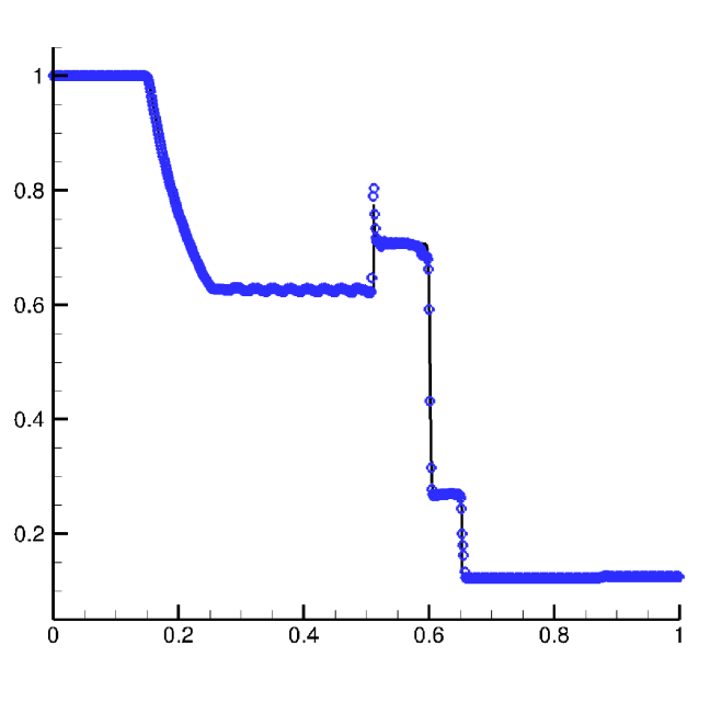
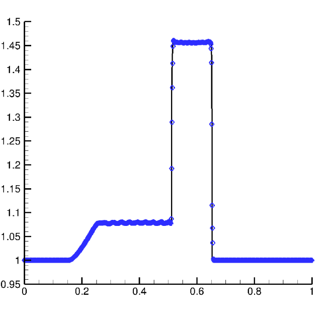
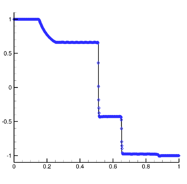
Figure 5.1: Example 5.2: The rest-mass density $\rho$, the Lorentz factor $W$, and the $y$ component of the magnetic field $B_{2}$ at $t=0.4$ with $N_{x}=800$ cells (from left to right). The symbol “$\circ$” and the solid line are the numerical and reference solutions, respectively.

Example 5.3 (Riemann problem II).

The initial data of the second 1D Riemann problem [81] are

$$(\rho,v_{1},v_{2},v_{3},B_{1},B_{2},B_{3},p)=\begin{cases}(1,~{}0,~{}0,~{}0,~{}5,~{}6,~{}6,~{}30),&\quad x<0.5,\\ (1,~{}0,~{}0,~{}0,~{}5,~{}0.7,~{}0.7,~{}1),&\quad x>0.5.\end{cases}$$

Figure 5.2 plots the rest-mass density $\rho$, the $x$ component of the velocity $v_{1}$, and the $y$ component of the magnetic field $B_{2}$ at $t=0.4$ obtained by the entropy stable DG scheme with $800$ cells and the TVB limiter ($M=10$). It can be seen that the solution consists of two left-moving rarefaction waves, a contact discontinuity, and two right-moving shock waves, and our scheme can still resolve the waves well, although small overshoot appears near the contact discontinuity.

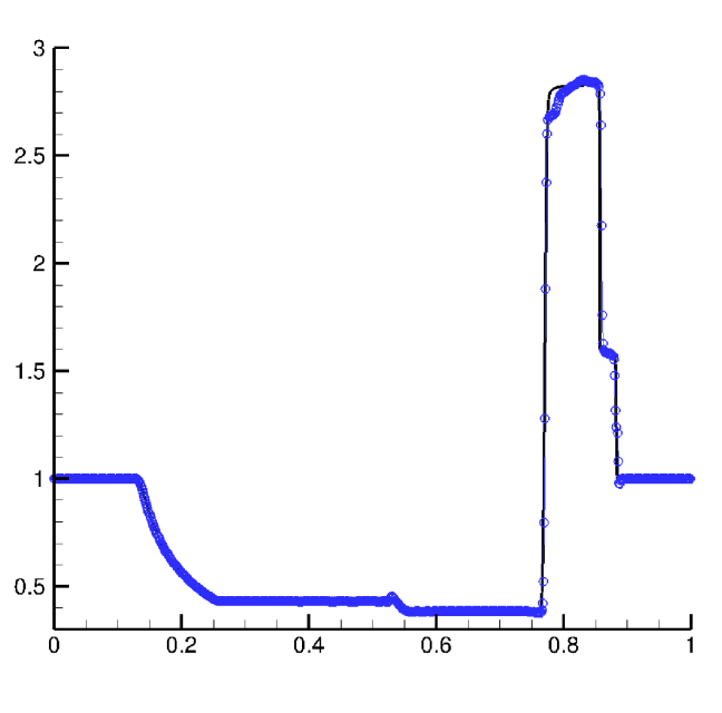
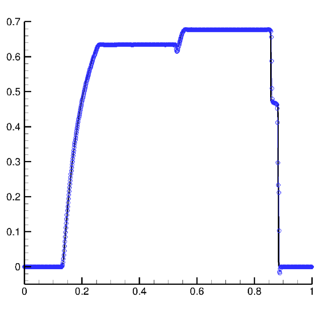
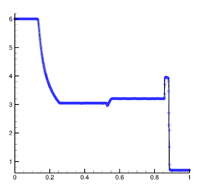
Figure 5.2: Example 5.3: The rest-mass density $\rho$, the $x$ component of the velocity $v_{1}$, and the $y$ component of the magnetic field $B_{2}$ at $t=0.4$ with $800$ cells (from left to right). The symbol “$\circ$” and the solid line are the numerical and reference solutions, respectively.

Example 5.4 (Riemann problem III).

The initial data of the third 1D Riemann problem [53] are

$$(\rho,v_{1},v_{2},v_{3},B_{1},B_{2},B_{3},p)=\begin{cases}(1,~{}0,~{}0.3,~{}0.4,~{}1,~{}6,~{}2,~{}5),&\quad x<0.5,\\ (0.9,~{}0,~{}0,~{}0,~{}1,~{}5,~{}2,~{}5.3),&\quad x>0.5.\end{cases}$$

The initial discontinuity will break into seven waves: a fast rarefaction wave, a rotational wave, and a slow shock wave moving to the left of the contact discontinuity, and a slow shock wave, an Alfvén wave, and a fast shock wave moving to the right of the contact discontinuity. Figure 5.3 shows the rest-mass density $\rho$, the $x$ component of the velocity $v_{1}$, and the $y$ component of the magnetic field $B_{2}$ at $t=0.4$ obtained by the entropy stable DG scheme with $800$ cells and the TVB limiter ($M=10$). From those plots, we can see that our scheme can capture the discontinuities well, as well as two narrow regions between the rotational wave at $x\approx 0.455$ and the slow shock wave at $x\approx 0.468$, and the slow shock wave at $x\approx 0.558$ and the Alfvén wave at $x\approx 0.565$.

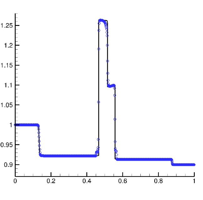
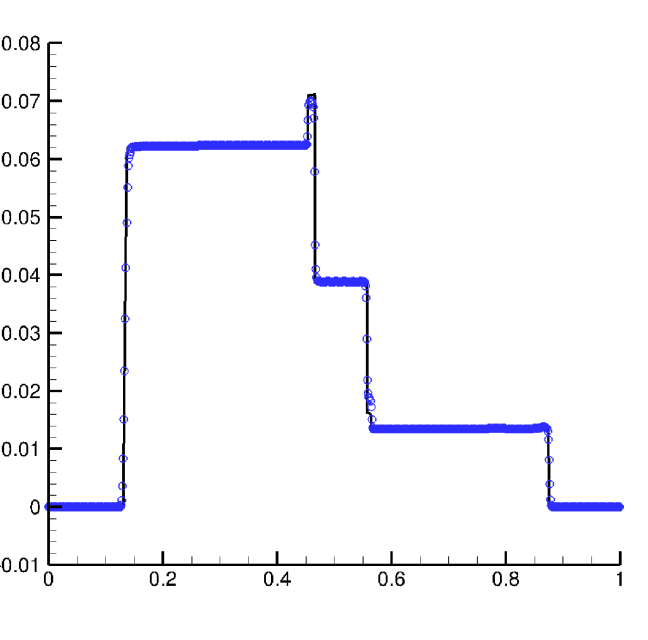
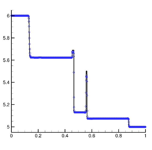
Figure 5.3: Example 5.4: The rest-mass density $\rho$, the $x$ component of the velocity $v_{1}$, and the $y$ component of the magnetic field $B_{2}$ at $t=0.4$ with $800$ cells (from left to right). The symbol “$\circ$” and the solid line are the numerical and reference solutions, respectively.

5.2 2D case

Example 5.5 (2D Alfvén wave).

This test is used to verify the accuracy of the 2D entropy stable scheme. The computational domain $[0,2/\sqrt{3}]\times[0,2]$ with periodic boundary conditions is divided into $N_{x}\times N_{y}$ uniform cells. A sine wave is propagating in the direction $(\sqrt{3}/2,1/2)$, i.e., the angle with the $x$-axis is $\alpha=\pi/6$. The exact solutions [81] are given by

$$\rho(x,y,t)=1,\quad v_{1}(x,y,t)=-0.1\sin(2\pi(\xi+t/\kappa))\sin\alpha,$$

$$v_{2}(x,y,t)=0.1\sin(2\pi(\xi+t/\kappa))\cos\alpha,\quad v_{3}(x,y,t)=0.1\cos(2\pi(\xi+t/\kappa)),$$

$$B_{1}(x,y,t)=\cos\alpha+\kappa v_{1}(x,y,t),\quad B_{2}(x,y,t)=\sin\alpha+\kappa v_{2}(x,y,t),$$

$$B_{3}(x,y,t)=\kappa v_{3}(x,y,t),\quad p(x,y,t)=0.1,$$

where $\xi=x\cos\alpha+y\sin\alpha,\kappa=\sqrt{1+\rho hW^{2}}$.

Table 5.2 lists the errors and the orders of convergence in $B_{2}$ at $t=1$ obtained by using our entropy stable DG scheme. It is seen that the orders of convergence are half order less than the optimal order. It is similar to the phenomenon observed in [12]. The possible reason is the inaccurate numerical quadrature rule used in the element.

$N_{x}=N_{y}$	$\ell^{1}$ error	order	$\ell^{2}$ error	order	$\ell^{\infty}$ error	order
10	4.180e-04	-	4.994e-04	-	1.608e-03	-
20	5.550e-05	2.91	6.741e-05	2.89	2.313e-04	2.80
40	7.054e-06	2.98	8.820e-06	2.93	2.896e-05	3.00
80	9.656e-07	2.87	1.192e-06	2.89	4.674e-06	2.63
160	1.526e-07	2.66	1.964e-07	2.60	7.962e-07	2.55

Table 5.2: Example 5.5: Errors and orders of convergence in $B_{2}$ at $t=1$.

Example 5.6 (Isentropic vortex).

The 2D relativistic isentropic vortex problem constructed in [3] is used to further test the accuracy and performance of our 2D scheme. The computational domain $[-5,5]^{2}$ with periodic boundary conditions is divided into $N_{x}\times N_{y}$ uniform cells. The setup of a steady vortex centered at $(0,0)$ in a coordinate system $S$ with the space-time coordinates $(t,x,y)$ is

$$(v_{1},v_{2})=v_{\text{max}}^{\phi}e^{0.5(1-r^{2})}(-y,x),$$

$$(B_{1},B_{2})=B_{\text{max}}^{\phi}e^{0.5(1-r^{2})}(-y,x),$$

with $v_{\text{max}}^{\phi}=B_{\text{max}}^{\phi}=0.7$ and $r=\sqrt{x^{2}+y^{2}}$. The vortex is isentropic so that $p=\rho^{\Gamma}$, and then the pressure can be solved by

$$r\dfrac{\mathrm{d}p_{\text{tot}}}{\mathrm{d}r}=\left(\rho h+\lvert b\rvert^{2}\right)W^{2}|v|^{2}-\lvert b\rvert^{2},\quad p_{\text{tot}}(0)=1.$$

Next, assume that a coordinate system $S^{\prime}$ with the spacetime coordinates $(t^{\prime},x^{\prime},y^{\prime})$ is in motion relative to the coordinate system $S$ with a constant velocity of magnitude $w$ along the $(1,1)$ direction, from the perspective of an observer stationary in $S$. The relationship between the coordinate systems $S$ and $S^{\prime}$ is given by the Lorentz transformation as follows

$$\gamma=\dfrac{1}{\sqrt{1-w^{2}}},\quad t=\gamma\big{(}t^{\prime}+\dfrac{w}{\sqrt{2}}(x^{\prime}+y^{\prime})\big{)},$$

$$x=x^{\prime}+\dfrac{\gamma-1}{2}(x^{\prime}+y^{\prime})+\dfrac{\gamma t^{\prime}w}{\sqrt{2}},\quad y=y^{\prime}+\dfrac{\gamma-1}{2}(x^{\prime}+y^{\prime})+\dfrac{\gamma t^{\prime}w}{\sqrt{2}}.$$

Corresponding transformations between the velocities and the magnetic field are given by

$$v_{1}^{\prime} =\dfrac{1}{1-\frac{w(v_{1}+v_{2})}{\sqrt{2}}}\left[\dfrac{v_{1}}{\gamma}-\dfrac{w}{\sqrt{2}}+\dfrac{\gamma w^{2}}{2(\gamma+1)}(v_{1}+v_{2})\right],$$

$$v_{2}^{\prime} =\dfrac{1}{1-\frac{w(v_{1}+v_{2})}{\sqrt{2}}}\left[\dfrac{v_{2}}{\gamma}-\dfrac{w}{\sqrt{2}}+\dfrac{\gamma w^{2}}{2(\gamma+1)}(v_{1}+v_{2})\right],$$

and

$$B_{1}^{\prime} =B_{1}+\frac{\gamma-1}{2}(B_{1}-B_{2}),$$

$$B_{2}^{\prime} =B_{2}-\frac{\gamma-1}{2}(B_{1}-B_{2}),$$

respectively. Using those transformations gives a time-dependent solution $(\rho^{\prime},v_{1}^{\prime},v_{2}^{\prime},B_{1}^{\prime},B_{2}^{\prime},p^{\prime})$ in the coordinate system $S^{\prime}$. This test describes a RMHD vortex moves with a constant speed of magnitude $w$ in $(-1,-1)$ direction.

We choose $w=0.5\sqrt{2}$, and the output time is $t=20$ so that the vortex travels and returns to the original position after a period. The errors in the mass density $D$ and corresponding orders of convergence listed in Table 5.3 show that the orders of convergence of the present entropy stable DG scheme are nearly $2.5$ as the mesh is refined. Figure 5.4 plots the contours of the rest-mass density $\rho$ and the magnitude of the magnetic field $|\bm{B}|$ with $40$ equally spaced contour lines. The results show that due to the Lorentz contraction, the vortex becomes elliptical, and our scheme can preserve the shape of the vortex well after a whole period. Figure 5.5 presents the evolutions of the total entropy $\int_{\Omega}\eta(\bm{U}_{i,j})\mathrm{d}x\mathrm{d}y$ with respect to the time obtained by the entropy stable DG scheme with different resolutions. We can see that the total entropy decay as expected and they converge as the resolution increases.

$N_{x}=N_{y}$	$\ell^{1}$ error	order	$\ell^{2}$ error	order	$\ell^{\infty}$ error	order
20	4.239e-02	-	1.142e-01	-	1.012e+00	-
40	6.172e-03	2.78	1.878e-02	2.60	2.151e-01	2.23
80	5.333e-04	3.53	1.971e-03	3.25	3.297e-02	2.71
160	6.180e-05	3.11	2.507e-04	2.97	5.476e-03	2.59
320	9.280e-06	2.74	4.221e-05	2.57	1.008e-03	2.44

Table 5.3: Example 5.6: Errors and orders of convergence in $D$ at $t=20$.

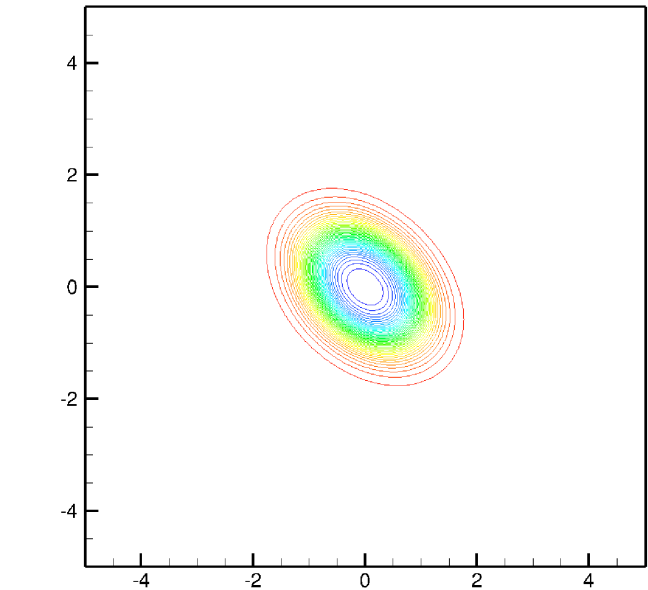
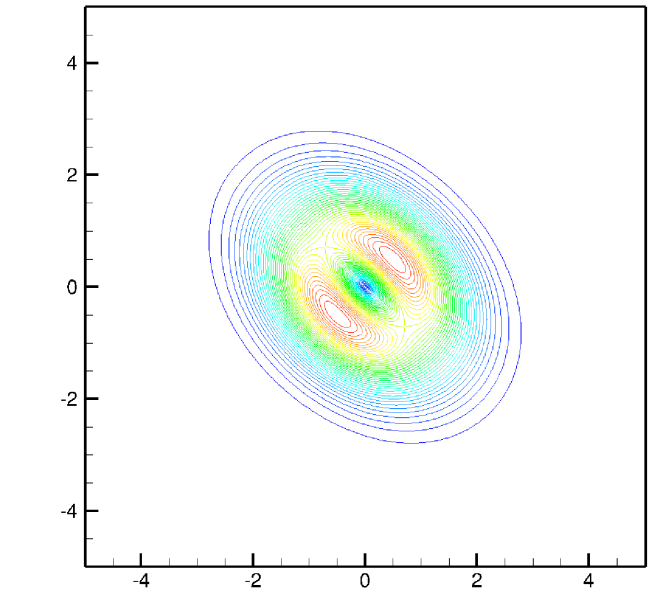
Figure 5.4: Example 5.6: The rest-mass density $\rho$ and the magnitude of the magnetic field $|B|$ (from left to right) at $t=20$ with $40$ equally spaced contour lines obtained by using the entropy stable scheme with $N_{x}=N_{y}=320$.

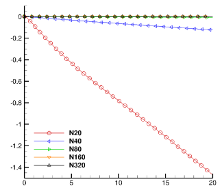
Figure 5.5: Example 5.6: The time evolution of the total entropy obtained by using the entropy stable DG scheme with different spatial resolutions of $N_{x}=N_{y}=20,40,80,160,320$.

Example 5.7 (Orszag-Tang problem).

It is a benchmark test for the RMHD equations [81]. The initial data are taken as follows

$${\rho(x,y,0)=\frac{25}{36\pi},\quad v_{1}(x,y,0)=0.5\sin(2\pi y),\quad v_{2}(x,y,0)=0.5\sin(2\pi x)},$$

$${v_{3}(x,y,0)=0,\quad B_{1}(x,y,0)=-\frac{1}{\sqrt{4\pi}}\sin(2\pi y),\quad B_{2}(x,y,0)=\frac{1}{\sqrt{4\pi}}\sin(4\pi x)},$$

$${B_{3}(x,y,0)=0,\quad p(x,y,0)=\frac{5}{12\pi}}.$$

The computational domain is $[0,1]^{2}$ with periodic boundary conditions. As time increases, complex wave patterns will emerge and the solution will present turbulent behavior.

In order to get a better performance of the nodal DG scheme, for this test and the following tests, we will first employ the KXRCF discontinuity indicator [38] to detect the “trouble cells”, and then use the TVB limiter to modify the nodal values in the “trouble cells”. Moreover, the physical-constraints-preserving limiter [71] is also used to guarantee that the numerical solutions are in the physical admissible state set. Figure 5.6 shows the contours of the rest-mass density $\rho$ and the Lorentz factor $W$ at $t=1$ with $40$ equally spaced contour lines with the TVB limiter parameter $M=10$. It can be seen that our scheme can resolve the wave patterns well and the results are comparable to those in [81].

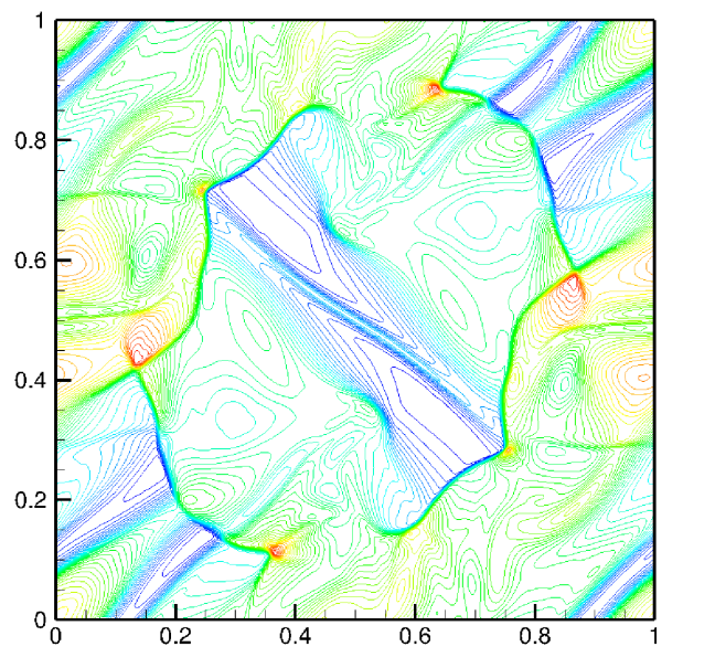
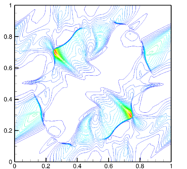
Figure 5.6: Example 5.7: The rest-mass density $\rho$ and the Lorentz factor $W$ (from left to right) at $t=1$ with $40$ equally spaced contour lines obtained by using the entropy stable scheme with $N_{x}=N_{y}=400$.

Example 5.8 (Blast problem).

It describes a 2D RMHD blast problem. The initial setup is the same as that in [3, 17, 51]. The computation domain $[-6,6]^{2}$ with outflow boundary conditions consists of three parts. The inner part is the explosion zone with a radius of $0.8$, and $\rho=0.01,~{}p=1$. The outer part is the ambient medium with the radius larger than $1$, and $\rho=10^{-4},~{}p=5\times 10^{-4}$. The intermediate part is a linear taper applied to the density and the pressure from the radius $0.8$ to $1$. The magnetic field is only initialized in the $x$-direction as $B_{1}=0.1$ or 0.5. The adiabatic index $\Gamma=4/3$ is used in this test.

Figures 5.7 and 5.8 plot the contours of the rest-mass density logarithm, the pressure logarithm, the Lorentz factor, and the magnitude of the magnetic field at $t=4$ with $40$ equally spaced contour lines obtained by using the entropy stable scheme with the TVB limiter parameter $M=0.01$. We can see that the solutions are well gotten and those for the case of $B_{1}=0.1$ and $0.5$ are in agreement with those in [3] and [71], respectively.

The time evolution of the total entropy in Example 5.7 and Example 5.8 is shown in Figure 5.9, and the observed monotonic decay implies that the fully discrete scheme is entropy stable.

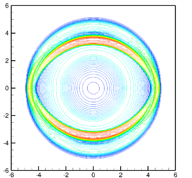
(a) $\log_{10}\rho$

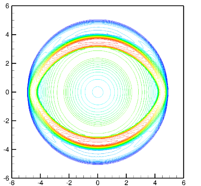
(b) $\log_{10}p$

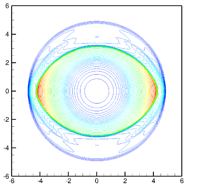
(c) $W$

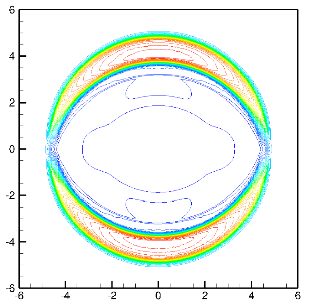
(d) $|\bm{B}|$

Figure 5.7: Example 5.8 with initial $B_{1}=0.1$: Numerical solutions at $t=4$ with $40$ equally spaced contour lines obtained by using the entropy stable scheme with $N_{x}=N_{y}=400$.

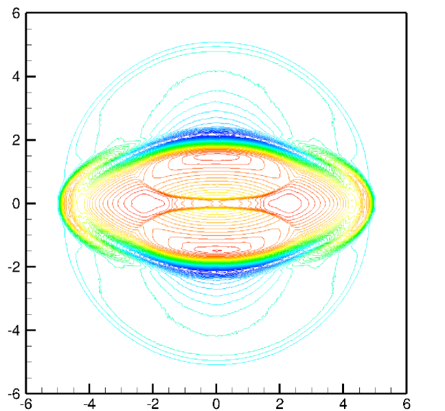
(a) $\log_{10}\rho$

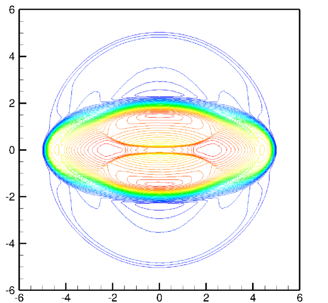
(b) $\log_{10}p$

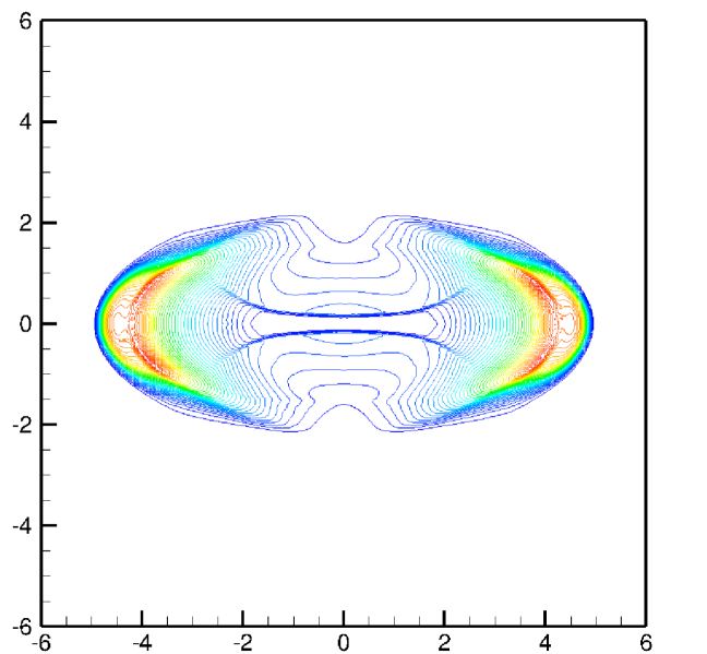
(c) $W$

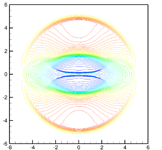
(d) $|\bm{B}|$

Figure 5.8: Same as Figure 5.7 except for the initial $B_{1}=0.5$.

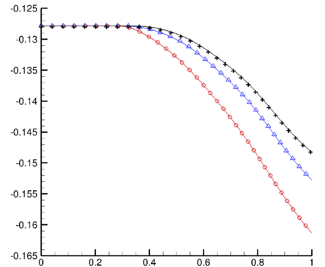
(a) Example 5.7.

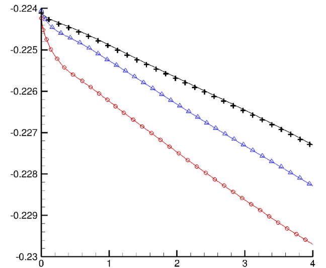
(b) Example 5.8 for the initial $B_{1}=0.1$.

Figure 5.9: The evolution of the total entropy obtained by using the entropy stable scheme. The symbols “$\circ$”, “$\Delta$”, and “$+$” with line denote the results obtained by using $100\times 100,200\times 200,400\times 400$ cells, respectively.

Example 5.9 (Shock-vortex interaction).

This test is about the interaction between a shock wave and a vortex, which is constructed in [3]. Here we rotate the shock wave and vortex clockwise by $\pi/4$, in order to eliminate the boundary effects in the computational domain. The present computational domain is taken as $[-9,9]^{2}$, and an isentropic vortex initially centered at $(-3,0)$, similar to that in Example 5.6, is put, except for $w=-0.6\sqrt{2}$. A planar stationary shock wave placed at $x=2\sqrt{2}-3$ is initially far away from the vortex so that the pre-shock state is a constant state

$$(\rho,v_{1},v_{2},B_{1},B_{2},p)=(6.73586072,~{}0.6\sqrt{2},~{}0,~{}0,~{}0,~{}24.02454458).$$

Following [3], the post-shock state is

$$(\rho,v_{1},v_{2},B_{1},B_{2},p)=(10.47090373,~{}0.507707117\sqrt{2},~{}0,~{}0,~{}0,~{}50.44557978),$$

when $x\geqslant 2\sqrt{2}-3$. The problem is solved until $t=10$, but the results at $t=3.4$ will also be given to show that the vortex is half-way through the shock wave.

Figure 5.10 plots the contours of $\rho,W,|\bm{B}|$ at $t=3.4,10$ with $40$ equally spaced contour lines obtained by using our entropy stable scheme with $N_{x}=N_{y}=600$ and the TVB limiter parameter $M=10$. Those results show that the shock wave is still located at $x=2\sqrt{2}-3$ after the interaction of the vortex and the shock wave, and our entropy stable scheme can capture the complicated structures of the solutions. They are very similar to those in [3], even though our result in the center of the vortex is not as smooth as that in [3].

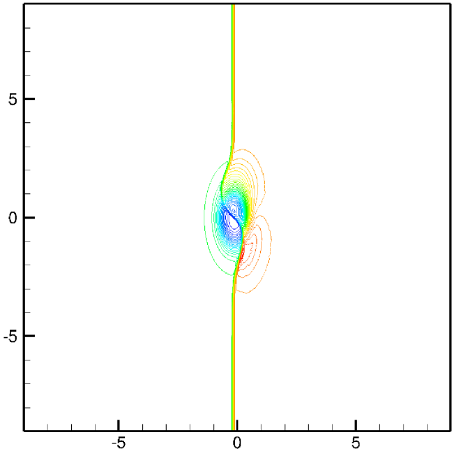
(a) $\rho$

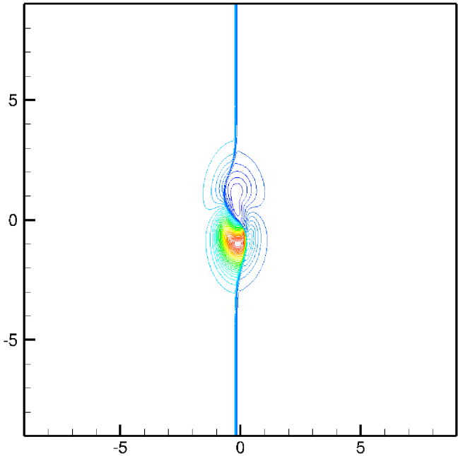
(b) $W$

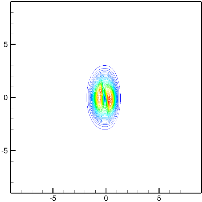
(c) $|\bm{B}|$

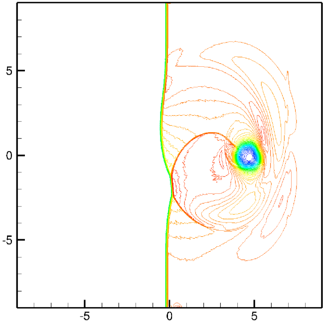
(d) $\rho$

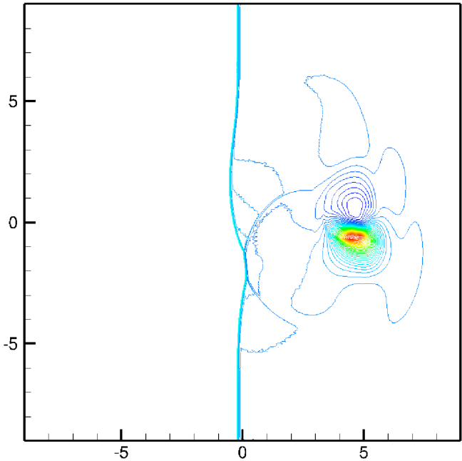
(e) $W$

(f) $|\bm{B}|$

Figure 5.10: Example 5.9: Numerical solutions at $t=3.4$ (first row) and $10$ (second row) with $40$ equally spaced contour lines obtained by using the entropy stable scheme with $N_{x}=N_{y}=600$.

5.3 Comparison between two entropy conservative fluxes

This section presents a numerical comparison of our two-point entropy conservative flux and that in [69]. As stated in Section 3, the parallel magnetic component of our entropy conservative flux is zero so that it is “fully consistent” with the physical flux. However, the parallel magnetic component of the entropy conservation flux in [69] is not zero, thus one can expect that the entropy stable DG scheme with our entropy conservative flux will behave better.

In the following, we take three 1D Riemann problems in Examples 5.2-5.4 and a rotated shock tube problem as examples.

Figure 5.11 shows the $B_{1}$ components for three 1D Riemann problems obtained by the entropy stable DG scheme using our two-point entropy conservative flux (3.16)-(3.18) and the flux (3.6) in [69], respectively. The other components are nearly the same so that they are omitted here and the only difference between two schemes is just in the two-point entropy conservative flux. The solid lines and the symbol (“$\square$”) denote the numerical solutions obtained by using the flux (3.16)-(3.18) and the flux (3.6) in [69], respectively. We can see that, for those Riemann problems, the results with the present two-point entropy conservative flux can maintain $B_{1}$ invariant exactly, while others do not have this property, and maintaining a zero parallel magnetic component is useful to reduce the error in the parallel magnetic component.

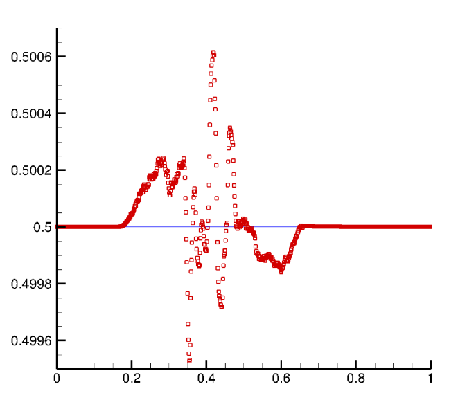
(a) Example 5.2

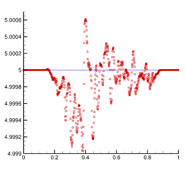
(b) Example 5.3

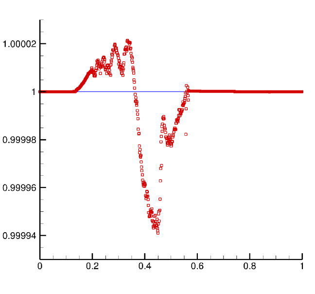
(c) Example 5.4

Figure 5.11: Examples 5.2-5.4: The solid line and the symbol (“$\square$”) denote the numerical solutions obtained by using the flux (3.16)-(3.18) and the flux (3.6) in [69], respectively.

Example 5.10 (Rotated shock tube).

Following [43, 63], this rotated shock tube problem is designed to compare the results of the entropy stable DG schemes with different two-point entropy conservative fluxes. The initial left and right states are $(\rho,v_{\parallel},v_{\perp},B_{\parallel},B_{\perp},p)=(1,~{}0.5,~{}0,~{}0.5,~{}0.5,~{}1)$ and $(1,-0.5,~{}0,~{}0.5,~{}0.5,~{}0.1)$, respectively. A $800\times 2$ Cartesian mesh with $\Delta x=\Delta y=1/800$ is used. The top and bottom boundaries are translational symmetry in the $(-1,1)$ direction, while the left and right boundary conditions are specified by the initial conditions, in view of the fact that the waves do not reach those boundaries at the output time $t=0.4$.

Figure 5.12 plots the numerical solutions obtained by using the entropy stable DG schemes, where the symbols “$\circ$” and “$+$” denote the numerical solutions obtained by using the flux (3.16)-(3.18) and the flux (3.6) in [69], respectively, and the solid line denotes the reference solution obtained by using a 1D first-order finite volume scheme on a mesh of $20000$ cells. Our numerical solutions are in good agreement with the reference solutions, except that the parallel component of the magnetic field $B_{\parallel}$ is not a constant due to the non-conservative source term, which can also be seen in [43, 63]. In this example, the schemes with two entropy conservative fluxes give similar results and the large error is shown in $B_{\parallel}$ when $\nabla\cdot{\bm{B}}$ is not zero. From this example, we can see that the error in $B_{\parallel}$ mainly results from the error in $\nabla\cdot{\bm{B}}$, which dominates the error in the non-zero parallel component of the two-point entropy conservative flux, thus we almost cannot distinguish the results in $B_{\parallel}$ in Figure 5.12. In summary, the newly resulting two-point entropy conservative flux may serve as a better base of the entropy conservative or stable schemes for the RMHD equations since it gives better or at least comparable results.

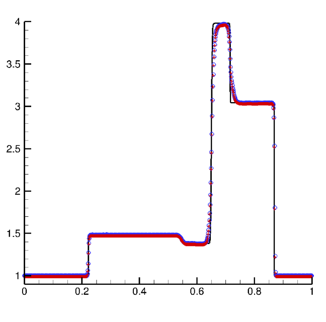
(a) $\rho$

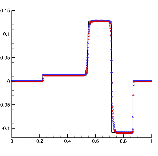
(b) $v_{\perp}$

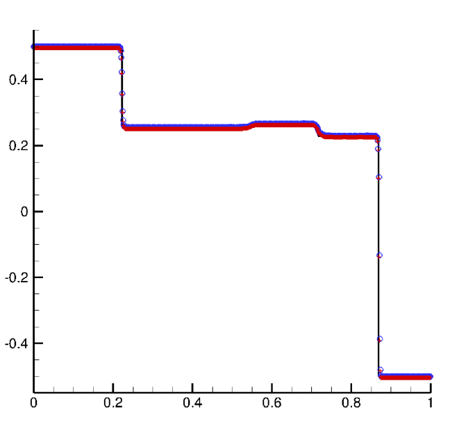
(c) $v_{\parallel}$

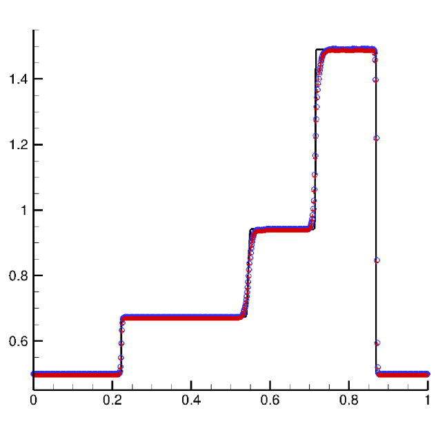
(d) $B_{\perp}$

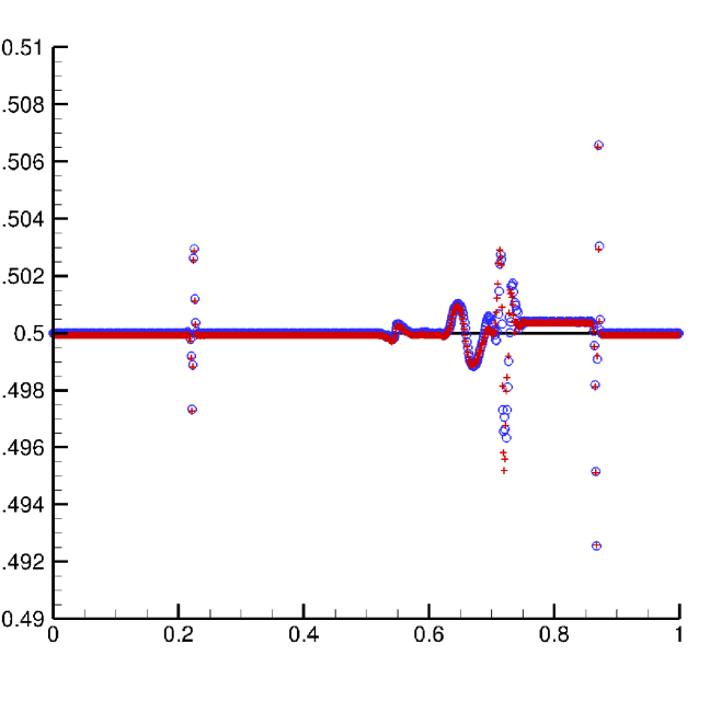
(e) $B_{\parallel}$

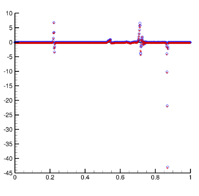
(f) $\nabla\cdot{\bm{B}}$

Figure 5.12: Example 5.10: The symbols “$\circ$” and “$+$” denote the numerical solutions obtained by using the flux (3.16)-(3.18) and the flux (3.6) in [69], respectively. The solid line is the reference solution.

6 Conclusion

This paper has presented the high-order accurate entropy stable nodal DG schemes for the ideal special RMHD equations. The conservative RMHD equations we usually considered cannot be symmetrized, thus a particular source term is added into the RMHD equations to achieve the symmetrization of the RMHD equations, and the corresponding convex entropy pair is found to symmetrize the modified RMHD equations. For the modified RMHD equations, high-order entropy stable DG schemes based on suitable quadrature rules are constructed to satisfy the semi-discrete entropy inequality for the given entropy pair. One key is to technically construct the affordable two-point entropy conservative flux, which is used inside each cell. Our two-point entropy conservative flux also maintains the zero parallel magnetic component, which is shown to be useful to reduce the errors in the parallel magnetic component in several one-dimensional Riemann problems, while in two dimensions, the entropy stable DG schemes with our two-point entropy conservative flux and with the existing two-point entropy conservative flux give comparable results in the rotated shock tube test, thus our newly derived entropy conservative flux may serve as a better base of the entropy conservative or the entropy stable schemes for the RMHD equations. At the cell interfaces, the entropy stable fluxes are used, resulting in an entropy stable DG schemes satisfying the semi-discrete entropy inequality. The semi-discrete schemes are integrated in time by using the high-order explicit Runge-Kutta schemes. Extensive numerical tests are conducted to validate the accuracy and the ability to capture discontinuities of our entropy stable DG schemes.

References

- [1] A. M. Anile and S. Pennisi, On the mathematical structure of test relativistic magnetofluiddynamics, Ann. Inst. Henri Poincaré, 46 (1987), 27-44.
- [2] L. Antón, J. A. Miralles, J. M. Martí, J. M. Ibáez, M. A. Aloy, and P. Mimica, Relativistic magnetohydrodynamics: Renormalized eigenvectors and full wave decomposition Riemann solver, Astrophys. J. Suppl. Ser., 188 (2010), 1-31.
- [3] D. S. Balsara and J. Kim, A subluminal relativistic magnetohydrodynamics scheme with ADER-WENO predictor and multidimensional Riemann solver-based corrector, J. Comput. Phys., 312 (2016), 357-384.
- [4] T. J. Barth, Numerical methods for gas-dynamics systems on unstructured meshes, in An Introduction to Recent Developments in Theory and Numerics of Conservation Laws, edited by D. Kroner, M. Ohlberger and C. Rohde, Lecture Notes in Comput. Sci. Engrg, volume 5, Berlin: Springer, 1999, 195-285.
- [5] K. Beckwith and J. M. Stone, A second-order Godunov method for multi-dimensional relativistic magnetohydrodynamics, Astrophys. J. Suppl. Ser., 193 (2011), 29pp.
- [6] B. Biswas and R. Dubey, Low dissipative entropy stable schemes using third order WENO and TVD reconstructions, Advan. Comput. Math., 44 (2018), 1153-1181.
- [7] R. Borges, M. Carmona, B. Costa, and W. S. Don, An improved weighted essentially non-oscillatory scheme for hyperbolic conservation laws, J. Comput. Phys., 227 (2008), 3191-3211.
- [8] F. Bouchut, C. Bourdarias, and B. Perthame, A MUSCL method satisfying all the numerical entropy inequalities, Math. Comp., 65 (1996), 1439-1461.
- [9] J. U. Brackbill and D. C. Barnes, The effect of nonzero on the numerical solution of the magnetohydrodynamic equations, J. Comput. Phys., 35 (1980), 426-430.
- [10] M. H. Carpenter, T. C. Fisher, E. J. Nielsen, and S. H. Frankel, Entropy stable spectral collocation schemes for the Navier-Stokes equations: discontinuous interfaces, SIAM J. Sci. Comput., 36 (2014), B835-B867.
- [11] P. Chandrashekar and C. Klingenberg, Entropy stable finite volume scheme for ideal compressible MHD on 2-D Cartesian meshes, SIAM J. Numer. Anal. 54 (2016), 1313-1340.
- [12] T. Chen and C.-W. Shu, Entropy stable high order discontinuous Galerkin methods with suitable quadrature rules for hyperbolic conservation laws, J. Comput. Phys., 345 (2017), 427-461.
- [13] Y. Cheng and C.-W. Shu, A discontinuous Galerkin finite element method for directly solving the Hamilton-Jacobi equations, J. Comput. Phys., 223 (2007), 398-415.
- [14] M. G. Crandall and A. Majda, Monotone difference approximations for scalar conservation laws, Math. Comp., 34 (1980), 1-21.
- [15] A. Dedner, F. Kemm, D. Kröner, C.-D. Munz, T. Schnitzer, and M. Wesenberg, Hyperbolic divergence cleaning for the MHD equations, J. Comput. Phys., 175 (2002), 645-673.
- [16] L. Del Zanna and N. Bucciantini, An efficient shock-capturing central-type scheme for multidimensional relativistic flows, I: Hydrodynamics, Astron. Astrophys., 390 (2002), 1177-1186.
- [17] L. Del Zanna, N. Bucciantini, and P. Londrillo, An efficient shock-capturing central-type scheme for multidimensional relativistic flows, II: Magnetohydrodynamics, Astron. Astrophys., 400 (2003), 397-413.
- [18] D. Derigs, A. R. Winters, G. J. Gassner, S. Walch, and M. Bohm, Ideal GLM-MHD: About the entropy consistent nine-wave magnetic field divergence diminishing ideal magnetohydrodynamics equations, J. Comput. Phys., 364 (2018), 420-467.
- [19] C. R. DeVore, Flux-corrected transport techniques for multidimensional compressible magnetohydrodynamics, J. Comput. Phys., 92 (1991), 142-160.
- [20] A. Dolezal and S. S. M. Wong, Relativistic hydrodynamics and essentially non-oscillatory shock capturing schemes, J. Comput. Phys., 120 (1995), 266-277.
- [21] J. M. Duan and H. Z. Tang, High-order accurate entropy stable finite difference schemes for one- and two-dimensional special relativistic hydrodynamics, accepted by Adv. Appl. Math. Mech., (2019), arXiv:1905.06092.
- [22] F. Eulderink and G. Mellema, General relativistic hydrodynamics with a Roe solver, Astron. Astrophys. Suppl. Ser., 110 (1995), 587-623.
- [23] C. R. Evans and J. F. Hawley, Simulation of magnetohydrodynamic flows: a constrained transport method, Astrophys. J., 332 (1988), 659-677.
- [24] T. C. Fisher and M. H. Carpenter, High-order entropy stable finite difference schemes for nonlinear conservation laws: Finite domains, J. Comput. Phys., 252 (2013), 518-557.
- [25] U. S. Fjordholm, S. Mishra, and E. Tadmor, Arbitrarily high-order accurate entropy stable essentially nonoscillatory schemes for systems of conservation laws, SIAM J. Numer. Anal., 50 (2012), 544-573.
- [26] U. S. Fjordholm, S. Mishra, and E. Tadmor, ENO reconstruction and ENO interpolation are stable, Found. Comput. Math., 13 (2013), 139-159.
- [27] J. A. Font, Numerical hydrodynamics and magnetohydrodynamics in general relativity, Living Rev. Relativ., 11 (2008), 7.
- [28] G. J. Gassner, A. R. Winters, and D. A. Kopriva, A well balanced and entropy conservative discontinuous Galerkin spectral element method for the shallow water equations, Appl. Math. Comput., 272 (2016), 291-308.
- [29] S. K. Godunov, The symmetric form of magnetohydrodynamics equation, Num. Meth. Mech. Cont. Media, 1 (1972), 26-34.
- [30] A. Harten, On a class of high-resolution TVD stable finite difference schemes, SIAM J. Numer. Anal., 21 (1984), 1-23.
- [31] P. He and H. Z. Tang, An adaptive moving mesh method for two-dimensional relativistic hydrodynamics, Commun. Comput. Phys., 11 (2012), 114-146.
- [32] P. He and H. Z. Tang, An adaptive moving mesh method for two-dimensional relativistic magnetohydrodynamics, Comput. Fluids, 60 (2012), 1-20.
- [33] A. Hiltebrand and S. Mishra, Entropy stable shock capturing space–time discontinuous Galerkin schemes for systems of conservation laws, Numer. Math., 126 (2014), 103-151.
- [34] T. J. Hughes, L. Franca, and M. Mallet, A new finite element formulation for computational fluid dynamics: I. Symmetric forms of the compressible Euler and Navier-Stokes equations and the second law of thermodynamics, Comput. Methods Appl. Mech. Eng., 54 (1986), 223-234.
- [35] F. Ismail and P. L. Roe, Affordable, entropy-consistent Euler flux functions II: Entropy production at shocks, J. Comput. Phys., 228 (2009), 5410-5436.
- [36] G. S. Jiang, C.-W. Shu, On a cell entropy inequality for discontinuous Galerkin methods, Math. Comp., 62 (1994), 531-538.
- [37] A. V. Koldoba, O. A. Kuznetsov, and G. V. Ustyugova, An approximate Riemann solver for relativistic magnetohydrodynamics, Mon. Not. R. Astron. Soc., 333 (2002), 932-942.
- [38] L. Krivodonova, J. Xin, J.-F. Remacle, N. Chevaugeon, and J. E. Flaherty, Shock detection and limiting with discontinuous Galerkin methods for hyperbolic conservation laws, Appl. Numer. Math., 48 (2004), 323-338.
- [39] P. G. LeFloch, J.-M. Mercier, and C. Rohde, Fully discrete, entropy conservative schemes of arbitrary order, SIAM J. Numer. Anal., 40 (2002), 1968-1992.
- [40] F. Y. Li and C.-W. Shu, Locally divergence-free discontinuous Galerkin methods for MHD equations, J. Sci. Comput., 22 (2005), 413-442.
- [41] F. Y. Li, L. W. Xu, and S. Yakovlev, Central discontinuous Galerkin methods for ideal MHD equations with the exactly divergence-free magnetic field, J. Comput. Phys., 230 (2011), 4828-4847.
- [42] D. Ling, J. M. Duan, and H. Z. Tang, Physical-constraints-preserving Lagrangian finite volume schemes for one- and two-dimensional special relativistic hydrodynamics, J. Comput. Phys., 396 (2019), 507-543.
- [43] Y. Liu, C.-W. Shu, and M. Zhang, Entropy stable high order discontinuous Galerkin methods for ideal compressible MHD on structured meshes, J. Comput. Phys., 354 (2018), 163-178.
- [44] J. M. Martí and E. Müller, Extension of the piecewise parabolic method to one-dimensional relativistic hydrodynamics, J. Comput. Phys., 123 (1996), 1-14.
- [45] J. M. Martí and E. Müller, Numerical hydrodynamics in special relativity, Living Rev. Relativ., 6 (2003), 7.
- [46] J. M. Martí and E. Müller, Grid-based methods in relativistic hydrodynamics and magnetohydrodynamics, Living Rev. Comput. Astrophys., 1 (2015), 3.
- [47] M. M. May and R. H. White, Hydrodynamics calculations of general-relativistic collapse, Phys. Rev., 141 (1966), 1232-1241.
- [48] M. M. May and R. H. White, Stellar dynamics and gravitational collapse, in Methods Comput. Phys., Vol. 7, edited by B. Alder, S. Fernbach, and M. Rotenberg, New York: Academic, 1967, 219-258.
- [49] M. L. Merriam, An entropy-based approach to nonlinear stability, NASA-TM-101086, 1989.
- [50] A. Mignone and G. Bodo, An HLLC Riemann solver for relativistic flows I - Hydrodynamics, Mon. Not. R. Astron. Soc., 364 (2005), 126-136.
- [51] A. Mignone and G. Bodo, An HLLC Riemann solver for relativistic flows II - Magnetohydrodynamics, Mon. Not. R. Astron. Soc., 368 (2006), 1040-1054.
- [52] A. Mignone, T. Plewa, and G. Bodo, The piecewise parabolic method for multidimensional relativistic fluid dynamics, Astron. Astrophys. Suppl. Ser., 160 (2005), 199-219.
- [53] A. Mignone, M. Ugliano, and G. Bodo, A five-wave Harten-Lax-van Leer Riemann solver for relativistic magnetohydrodynamics, Mon. Not. R. Astron. Soc., 393 (2009), 1141-1156.
- [54] P. Mösta et al., GRHydro: A new open-source general-relativistic magnetohydrodynamics code for the Einstein toolkit, Classical and Quantum Gravity, 31 (2014), 50pp.
- [55] J. Núez-de la Rosa and C. D. Munz, XTROEM-FV: A new code for computational astrophysics based on very high order finite-volume methods - II. Relativistic hydro- and magnetohydrodynamics, Mon. Not. R. Astron. Soc., 460 (2016), 535-559.
- [56] S. Osher, Riemann solvers, the entropy condition, and difference approximations, SIAM J. Numer. Anal., 21 (1984), 217-235.
- [57] S. Osher and E. Tadmor, On the convergence of difference approximations to scalar conservation laws, Math. Comp., 50 (1988), 19-51.
- [58] K. Powell, An approximate Riemann solver for magnetohydrodynamics (that works in more than one dimension), Tech. 94-24, ICASE, NASA Langley, 1994.
- [59] T. Qin, C.-W. Shu, and Y. Yang, Bound-preserving discontinuous Galerkin methods for relativistic hydrodynamics, J. Comput. Phys., 315 (2016), 323-347.
- [60] V. Schneider, U. Katscher, D. H. Rischke, B. Waldhauser, J. A. Maruhn, and C. D. Munz, New algorithms for ultra-relativistic numerical hydrodynamics, J. Comput. Phys., 105 (1993), 92-107.
- [61] E. Tadmor, The numerical viscosity of entropy stable schemes for systems of conservation laws, I. Math. Comp., 49 (1987), 91-103.
- [62] E. Tadmor, Entropy stability theory for difference approximations of nonlinear conservation laws and related time-dependent problems, Acta. Numer., (2004), 451-512.
- [63] G. Tóth, The constraint in shock-capturing magnetohydrodynamics codes, J. Comput. Phys., 161 (2000), 605-652.
- [64] J. R. Wilson, Numerical study of fluid flow in a Kerr space, Astrophys. J., 173 (1972), 431-438.
- [65] A. R. Winters and G. J. Gassner, Affordable, entropy conserving and entropy stable flux functions for the ideal MHD equations, J. Comput. Phys, 304 (2016), 72-108.
- [66] K. L. Wu, Design of provably physical-constraint-preserving methods for general relativistic hydrodynamics, Phys. Rev. D, 95 (2017), 103001.
- [67] K. L. Wu, Positivity-preserving analysis of numerical schemes for ideal magnetohydrodynamics, SIAM J. Numer, Anal., 56 (2018), 2124-2147.
- [68] K. L. Wu and C.-W. Shu, A provably positive discontinuous Galerkin method for multidimensional ideal magnetohydrodynamics, SIAM J. Sci. Comput., 40 (2018), B1302-B1329.
- [69] K. L. Wu and C.-W. Shu, Entropy symmetrization and high-order accurate entropy stable numerical schemes for relativistic MHD equations, arXiv:1907.07467, (2019).
- [70] K. L. Wu and H. Z. Tang, A direct Eulerian GRP scheme for spherically symmetric general relativistic hydrodynamics, SIAM J. Sci. Comput., 38 (2016), B458-B489.
- [71] K. L. Wu and H. Z. Tang, Admissible states and physical constraints preserving numerical schemes for special relativistic magnetohydrodynamics, Math. Mod. Meth. Appl. Sci., 27 (2017), 1871-1928.
- [72] K. L. Wu and H. Z. Tang, High-order accurate physical-constraints-preserving finite difference WENO schemes for special relativistic hydrodynamics, J. Comput. Phys., 298 (2015), 539-564.
- [73] K. L. Wu and H. Z. Tang, On physical-constraints-preserving schemes for special relativistic magnetohydrodynamics with a general equation of state, Z. Angew. Math. Phys., 69 (2018), 84.
- [74] K. L. Wu and H. Z. Tang, Physical-constraints-preserving central discontinuous Galerkin methods for special relativistic hydrodynamics with a general equation of state, Astrophys. J. Suppl. Ser., 228 (2017), 3.
- [75] K. L. Wu, Z. C. Yang, and H. Z. Tang, A third-order accurate direct Eulerian GRP scheme for one-dimensional relativistic hydrodynamics, East Asian J. Appl. Math., 4 (2014), 95-131.
- [76] Z. C. Yang, P. He, and H. Z. Tang, A direct Eulerian GRP scheme for relativistic hydrodynamics: one-dimensional case, J. Comput. Phys., 230 (2011), 7964-7987.
- [77] Z. C. Yang and H. Z. Tang, A direct Eulerian GRP scheme for relativistic hydrodynamics: two-dimensional case, J. Comput. Phys., 231 (2012), 2116-2139.
- [78] Y. H. Yuan and H. Z. Tang, Two-stage fourth-order accurate time discretizations for 1D and 2D special relativistic hydrodynamics, accepted by J. Comput. Math., (2019), arXiv:1712.05546.
- [79] W. Q. Zhang and A. I. MacFadyen, RAM: A relativistic adaptive mesh refinement hydrodynamics code, Astrophys. J. Suppl. Ser., 164 (2006), 255-279.
- [80] J. Zhao and H. Z. Tang, Runge-Kutta discontinuous Galerkin methods with WENO limiter for the special relativistic hydrodynamics, J. Comput. Phys., 242 (2013), 138-168.
- [81] J. Zhao and H. Z. Tang, Runge-Kutta discontinuous Galerkin methods for the special relativistic magnetohydrodynamics, J. Comput. Phys., 343 (2017), 33-72.