Einsteinโ€™s $E=mc^{2}$ derivable
from Heisenbergโ€™s Uncertainty Relations

Sibel BaลŸkal

Department of Physics, Middle East Technical University, 06800 Ankara, Turkey

Young S. Kim

Center for Fundamental Physics, University of Maryland College Park,

Maryland, 20742, USA

Marilyn E. Noz

Department of Radiology, New York University, New York, NY 10016, USA

Abstract

Heisenbergโ€™s uncertainty relation can be written in terms of the step-up and step-down operators in the harmonic oscillator representation. It is noted that the single-variable Heisenberg commutation relation contains the symmetry of the $Sp(2)$ group which is isomorphic to the Lorentz group applicable to one time-like dimension and two space-like dimensions, known as the $O(2,1)$ group. This group has three independent generators. The one-dimensional step-up and step-down operators can be combined into one two-by-two Hermitian matrix which contains three independent operators. If we use a two-variable Heisenberg commutation relation, the two pairs of independent step-up, step-down operators can be combined into a four-by-four block-diagonal Hermitian matrix with six independent parameters. It is then possible to add one off-diagonal two-by-two matrix and its Hermitian conjugate to complete the four-by-four Hermitian matrix. This off-diagonal matrix has four independent generators. There are thus ten independent generators. It is then shown that these ten generators can be linearly combined to the ten generators for the Diracโ€™s two oscillator system leading to the group isomorphic to the de Sitter group $O(3,2)$, which can then be contracted to the inhomogeneous Lorentz group with four translation generators corresponding to the four-momentum in the Lorentz-covariant world. This Lorentz-covariant four-momentum is known as Einsteinโ€™s $E=mc^{2}.$

Based on an invited paper presented by Young S. Kim at the 16th International Conference on Squeezed States and Uncertainty Relations (Madrid, Spain, 2019); published in the Quantum Reports, Vol. 1 (2), 236 - 251 (2019), https://www.mdpi.com/2624-960X/1/2/21.

1 Introduction

Let us start with Heisenbergโ€™s commutation relations

$$\left[x_{i},P_{j}\right]=i~{}\delta_{ij},$$ (1)

with

$$P_{i}=-i\frac{\partial}{\partial x_{i}},$$ (2)

where $i=1,2,3,$ correspond to the $x,y,z$ coordinates respectively.

With these $x_{i}$ and $P_{i}$, we can construct the following three operators,

$$J_{i}=\epsilon_{ijk}x_{j}P_{k}.$$ (3)

These three operators satisfy the closed set of commutation relations:

$$\left[J_{i},J_{j}\right]=i\epsilon_{ijk}J_{k}.$$ (4)

These $J_{i}$ operators generate rotations in the three-dimensional space. In mathematics, this set is called the Lie algebra of the rotation group. This is a direct consequence of Heisenbergโ€™s commutation relations.

In quantum mechanics, each $J_{i}$ corresponds to the angular momentum along the $i$ direction. The remarkable fact is that it is also possible to construct the same Lie algebra with two-by-two matrices. These matrices are of course the Pauli spin matrices, leading to the observable angular momentum not seen in classical mechanics.

As the expression shows in Eq.(2), each $P_{i}$ generates a translation along the $i^{th}$ direction. Thus, the three translation generators, together with the three rotation generators constitute the Lie algebra of the Galilei group, with the additional commutation relations:

$$\left[J_{i},P_{j}\right]=i\epsilon_{ijk}P_{k}.$$ (5)

This set of commutation relations together with those of Eq.(4) constitute a closed set for both $P_{i}$ and $J_{i}$. This set is called the Lie algebra of the Galilei group. This group is the basic symmetry group for the Schrรถdinger or non-relativistic quantum mechanics.

In the Schrรถdinger picture, the generator $P_{i}$ corresponds to the particle momentum along the $i$ direction. In addition, the time translation operator is

$$P_{0}=i\frac{\partial}{\partial t}.$$ (6)

This corresponds to the energy variable.

Let us go to the Lorentzian world. Here we have to take into account the generators of the boosts. The generators thus include the time variable, and the generator of boosts along the $i$ direction is

$$K_{i}=i\left(x_{i}\frac{\partial}{\partial t}+t\frac{\partial}{\partial x_{i}}\right).$$ (7)

These generators satisfy the commutation relations

$$\left[K_{i},K_{j}\right]=-i\epsilon_{ijk}J_{k}.$$ (8)

Thus, these three boost generators alone cannot constitute a closed set of commutation relations (Lie algebra).

With $J_{i}$, these boost generators satisfy

$$\left[J_{i},K_{j}\right]=i~{}\epsilon_{ijk}K_{k}.$$ (9)

With $P_{i}$, they satisfy the relation

$$\left[P_{i},K_{i}\right]=i\delta_{0i}P_{0}.$$ (10)

Thus, the commutation relations of Eqs.(4,5, 8,9,10) constitute a closed set of the ten generators. This closed set is commonly called the Lie algebra of the Poincarรฉ symmetry.

The three rotation and three translation generators are contained in or derivable from Heisenbergโ€™s commutation relations, and the time translation operator is seen in the Schrรถdinger equation. They are all Hermitian operators corresponding to dynamical variables. On the other hand, the three boost generators of Eq.(7) are not derivable from the Heisenberg relations. Furthermore, they do not appear to correspond to observable quantitiesย [1].

The purpose of this paper is to show that the Lie algebra of the Poincarรฉ symmetry is derivable from the Heisenberg commutation relations. For this purpose, we first examine the symmetry of the Heisenberg commutation relation using the Wigner function in the phase space. It is noted that the single-variable relation contains the symmetry of the Lorentz group applicable to two space-like and one time-like dimensions.
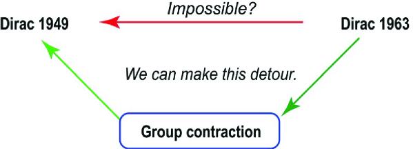
As Dirac noted in 1963ย [2], two coupled oscillators lead to the symmetry of the $O(3,2)$ or the Lorentz group applicable to the three space-like directions and two time-like directions. As is illustrated in Fig.ย 3, it is possible to contract one of those two time variables of this $O(3,2)$ group into the inhomogeneous Lorentz group consisting of the Lorentz group applicable to the three space-like dimensions and one time-like direction, plus four translation generators corresponding to the energy-momentum four-vector. This of course leads to Einsteinโ€™s energy-momentum relation of $E=mc^{2}$.

Refer to caption

Figure 1: According to Diracโ€™s 1949 paper, the task of constructing quantum mechanics is essentially constructing a representation of the inhomogeneous Lorentz group. In his 1963 paper, Dirac constructed the Lie algebra of the $O(3,2)$ de Sitter group from the algebra of two harmonic oscillators, which is a direct consequence of Heisenbergโ€™s uncertainty commutation relations. It is possible to derive the Lie algebra of the inhomogeneous Lorentz group from that of $O(3,2)$ using the group-contraction procedure of Inรถnรผ and Wignerย [3].

In Sec.ย 2, it is noted that the best way to study the symmetry of the Heisenberg commutation relation is to use the Wigner function for the Gaussian function for the oscillator state. In the Wigner phase space, this function contains the symmetry for the Lorentz group applicable to two space-like dimensions and one time-like dimension. This group has three generators. This operation is equivalent to constructing a two-by-two block-diagonal Hermitian matrix with quadratic forms of the step-up and step-down operators.

In Sec.ย 3, we consider two oscillators. If these oscillators are independent, it is possible to construct a four-by-four block diagonal matrix, where each block consists of the two-by-two matrix for each operator defined in Sec.ย 2. Since the oscillators are uncoupled, this four-by-four block-diagonal Hermitian matrix contains six independent generators.

If the oscillators are coupled, then to keep the overall four-by-four block-diagonal matrix Hermitian, we need one off-diagonal block matrix, with four independent quadratic forms. Thus, the overall four-by-four matrix contains ten independent quadratic forms of the creation and annihilation operators.

It is shown that these ten independent generators can be linearly combined into the ten generators constructed by Dirac for the the Lorentz-group applicable to three space-like dimensions and two time-like dimensions, commonly called $O(3,2)$ group.

In Sec.ย 4, using the boosts belonging to one of its time-like dimensions, we contract $O(3,2)$ to produce the Lorentz group applicable to one time dimension and four translations leading to the four-momentum. This Lorentz-covariant four-momentum is commonly known as Einsteinโ€™s $E=mc^{2}$.

This paper is basically based on Diracโ€™s paper published in 1949 and 1963ย [1, 2]. As is illustrated in Fig.1, we show here that the space-time symmetry of quantum mechanics mentioned in his 1949 paper is derivable from his two-oscillator system discussed in 1963. The route is the group contraction procedure of Inรถnรผ and Wignerย [3].

Indeed, Dirac made his lifelong efforts to synthesize quantum mechanics and special relativity from 1927ย [4]. In and before 1949, he treated quantum mechanics and special relativity as two separate scientific disciplines, and he then attempted to synthesized them. Thus, it is of interest to see how Diracโ€™s idea evolved during the period 1929-49. We shall give a brief review of Diracโ€™s efforts during the period in the Appendix.

2 Symmetries of the Single-mode States

Heisenbergโ€™s uncertainty relation for a single Cartesian variable takes the form

$$[x,p]=i.$$ (11)

with

$$p=-i\frac{\partial}{\partial x}.$$

Very often, it is more convenient to use the operators

a=12โ€‹(x+iโ€‹p),aโ€ =12โ€‹(xโˆ’iโ€‹p)formulae-sequence๐‘Ž12๐‘ฅ๐‘–๐‘superscript๐‘Žโ€ 12๐‘ฅ๐‘–๐‘a=\frac{1}{\sqrt{2}}(x+ip),\qquad a^{{\dagger}}=\frac{1}{\sqrt{2}}(x-ip) (12)

with

[a,aโ€ ]=1.๐‘Žsuperscript๐‘Žโ€ 1\left[a,a^{{\dagger}}\right]=1. (13)

This aspect is well known.

The representation based on $a$ and aโ€ superscript๐‘Žโ€ a^{{\dagger}} is known as the harmonic oscillator representation of the uncertainty relation and is the basic language for the Fock space for particle numbers. This representation is therefore the basic language for quantum optics.

Let us next consider the quadratic forms: aโ€‹a,aโ€ โ€‹aโ€ ,aโ€‹aโ€ ๐‘Ž๐‘Žsuperscript๐‘Žโ€ superscript๐‘Žโ€ ๐‘Žsuperscript๐‘Žโ€ aa,a^{{\dagger}}a^{{\dagger}},aa^{{\dagger}}, and aโ€ โ€‹asuperscript๐‘Žโ€ ๐‘Ža^{{\dagger}}a. Then the linear combination

aโ€‹aโ€ โˆ’aโ€ โ€‹a=1,๐‘Žsuperscript๐‘Žโ€ superscript๐‘Žโ€ ๐‘Ž1aa^{{\dagger}}-a^{{\dagger}}a=1, (14)

according to the uncertainty relation. Thus, there are three independent quadratic forms, and we are led to the following two-by-two matrix:

((aโ€‹aโ€ +aโ€ โ€‹a)/2aโ€‹aaโ€ โ€‹aโ€ (aโ€‹aโ€ +aโ€ โ€‹a)/2).matrix๐‘Žsuperscript๐‘Žโ€ superscript๐‘Žโ€ ๐‘Ž2๐‘Ž๐‘Žsuperscript๐‘Žโ€ superscript๐‘Žโ€ ๐‘Žsuperscript๐‘Žโ€ superscript๐‘Žโ€ ๐‘Ž2\pmatrix{\left(aa^{{\dagger}}+a^{{\dagger}}a\right)/2&aa\cr a^{{\dagger}}a^{{\dagger}}&\left(aa^{{\dagger}}+a^{{\dagger}}a\right)/2}. (15)

This matrix leads to the following three independent operators:

J2=12โ€‹(aโ€‹aโ€ +aโ€ โ€‹a),K1=12โ€‹(aโ€ โ€‹aโ€ +aโ€‹a),K3=i2โ€‹(aโ€ โ€‹aโ€ โˆ’aโ€‹a).formulae-sequencesubscript๐ฝ212๐‘Žsuperscript๐‘Žโ€ superscript๐‘Žโ€ ๐‘Žformulae-sequencesubscript๐พ112superscript๐‘Žโ€ superscript๐‘Žโ€ ๐‘Ž๐‘Žsubscript๐พ3๐‘–2superscript๐‘Žโ€ superscript๐‘Žโ€ ๐‘Ž๐‘ŽJ_{2}=\frac{1}{2}\left(aa^{{\dagger}}+a^{{\dagger}}a\right),\quad K_{1}=\frac{1}{2}\left(a^{{\dagger}}a^{{\dagger}}+aa\right),\quad K_{3}=\frac{i}{2}\left(a^{{\dagger}}a^{{\dagger}}-aa\right). (16)

They produce the following set of closed commutation relations:

$$\left[J_{2},K_{1}\right]=-iK_{3},\qquad\left[J_{2},K_{3}\right]=iK_{1},\qquad\left[K_{1},K_{3}\right]=iJ_{2}.$$ (17)

This set is commonly called the Lie algebra of the $Sp(2)$ group, locally isomorphic to the Lorentz group applicable to one time and two space coordinates.

The best way to study the symmetry property of these operators is to use the Wigner function for the ground-state oscillator which takes the formย [5, 6, 7, 8]

$$W(x,p)=\frac{1}{\pi}\exp\left[-\left(x^{2}+p^{2}\right)\right].$$ (18)

This distribution is concentrated in the circular region around the origin. Let us define the circle as

$$x^{2}+p^{2}=1.$$ (19)

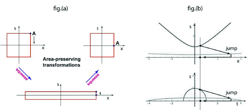
We can use the area of this circle in the phase space of $x$ and $p$ as the minimum uncertainty. This uncertainty is preserved under rotations in the phase space and also under squeezing. These transformations can be written as

$$\pmatrix{\cos\theta&-\sin\theta\cr\sin\theta&\cos\theta}\pmatrix{x\cr p},\qquad\pmatrix{e^{\eta}&0\cr 0&e^{-\eta}}\pmatrix{x\cr p},$$ (20)

respectively. The rotation and the squeeze are generated by

$$J_{2}=-i\left(x\frac{\partial}{\partial p}-p\frac{\partial}{\partial x}\right),\qquad K_{1}=-i\left(x\frac{\partial}{\partial x}-p\frac{\partial}{\partial p}\right).$$ (21)

If we take the commutation relation with these two operators, the result is

$$\left[J_{2},K_{1}\right]=-iK_{3},$$ (22)

with

$$K_{3}=-i\left(x\frac{\partial}{\partial p}+p\frac{\partial}{\partial x}\right).$$ (23)

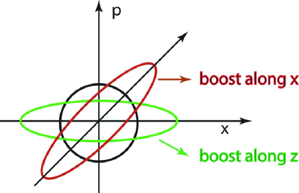
Indeed, as before, these three generators form the closed set of commutation which form the Lie algebra of the $Sp(2)$ group, isomorphic to the Lorentz group applicable to two space and one time dimensions. This isomorphic correspondence is illustrated in Fig.ย 2.

Refer to caption

Figure 2: Rotations and squeezes in the phase space produced by the $Sp(2)$ transformations. The squeeze along the $x$ direction corresponds to the Lorentz boost along the $z$ direction, while the squeeze along the $45^{o}$ degree corresponds to the boost along the $x$ direction. The rotation by $45^{o}$ corresponds to the rotation by $90^{o}$ around the $y$ axis.

Let us consider the Minkowski space of $(x,y,z,t)$. It is possible to write three four-by-four matrices satisfying the Lie algebra of Eq.(17). The three four-by-four matrices satisfying this set of commutation relations are:

$$J_{2}=\pmatrix{0&0&i&0\cr 0&0&0&0\cr i&0&0&0\cr 0&0&0&0},\quad K_{1}=\pmatrix{0&0&0&i\cr 0&0&0&0\cr 0&0&0&0\cr i&0&0&0},\quad K_{3}=\pmatrix{0&0&0&0\cr 0&0&0&0\cr 0&0&0&i\cr 0&0&i&0}.$$ (24)

However, these matrices have null second rows and null second columns. Thus, they can generate Lorentz transformations applicable only to the three-dimensional space of $(x,z,t)$, while the $y$ variable remains invariant. Thus, this single-oscillator system cannot describe what happens in the full four-dimensional Minkowski space.

Yet, it is interesting, the oscillator system can produce three different representations sharing the same Lie algebra with the (2 + 1)-dimensional Lorentz group, as shown in Tableย 1.

Table 1: Transformation for the Gaussian function, in terms of harmonic oscillators, two-dimensional phase space, and the four-dimensional Minkowski space.
Generators Oscillator Phase space Lorentz
$J_{2}$ 12โ€‹(aโ€‹aโ€ +aโ€ โ€‹a)12๐‘Žsuperscript๐‘Žโ€ superscript๐‘Žโ€ ๐‘Ž{1\over 2}\left(aa^{{\dagger}}+a^{{\dagger}}a\right) $\frac{1}{2}\sigma_{2}$ $\pmatrix{0&0&i&0\cr 0&0&0&0\cr i&0&0&0\cr 0&0&0&0}$
$K_{1}$ 12โ€‹iโ€‹(aโ€ โ€‹aโ€ +aโ€‹a)12๐‘–superscript๐‘Žโ€ superscript๐‘Žโ€ ๐‘Ž๐‘Ž{1\over 2i}\left(a^{{\dagger}}a^{{\dagger}}+aa\right) $\frac{i}{2}\sigma_{1}$ $\pmatrix{0&0&0&i\cr 0&0&0&0\cr 0&0&0&0\cr i&0&0&0}$
$K_{3}$ 12โ€‹(aโ€ โ€‹aโ€ โˆ’aโ€‹a),12superscript๐‘Žโ€ superscript๐‘Žโ€ ๐‘Ž๐‘Ž{1\over 2}\left(a^{{\dagger}}a^{{\dagger}}-aa\right), $\frac{i}{2}\sigma_{3}$ $\pmatrix{0&0&0&0\cr 0&0&0&0\cr 0&0&0&i\cr 0&0&i&0}$

3 Symmetries from Two Oscillators

In order to generate Lorentz transformations applicable to the full Minkowskian space, we may need two Heisenberg commutation relations. Indeed, Paul A. M. Dirac started this program in 1963ย [2]. It is possible to write the two uncertainty relations using two harmonic oscillators as

[ai,ajโ€ ]=ฮดiโ€‹j,subscript๐‘Ž๐‘–subscriptsuperscript๐‘Žโ€ ๐‘—subscript๐›ฟ๐‘–๐‘—\left[a_{i},a^{{\dagger}}_{j}\right]=\delta_{ij}, (25)

with

ai=12โ€‹(xi+iโ€‹pi),aiโ€ =12โ€‹(xiโˆ’iโ€‹pi),formulae-sequencesubscript๐‘Ž๐‘–12subscript๐‘ฅ๐‘–๐‘–subscript๐‘๐‘–subscriptsuperscript๐‘Žโ€ ๐‘–12subscript๐‘ฅ๐‘–๐‘–subscript๐‘๐‘–a_{i}=\frac{1}{\sqrt{2}}\left(x_{i}+ip_{i}\right),\qquad a^{{\dagger}}_{i}=\frac{1}{\sqrt{2}}\left(x_{i}-ip_{i}\right), (26)

and

xi=12โ€‹(ai+aiโ€ ),pi=i2โ€‹(aiโ€ โˆ’ai),formulae-sequencesubscript๐‘ฅ๐‘–12subscript๐‘Ž๐‘–subscriptsuperscript๐‘Žโ€ ๐‘–subscript๐‘๐‘–๐‘–2subscriptsuperscript๐‘Žโ€ ๐‘–subscript๐‘Ž๐‘–x_{i}=\frac{1}{\sqrt{2}}\left(a_{i}+a^{{\dagger}}_{i}\right),\qquad p_{i}=\frac{i}{\sqrt{2}}\left(a^{{\dagger}}_{i}-a_{i}\right), (27)

where $i$ and $j$ could be 1 or 2.

As in the case of the two-by-two matrix given in Eq.ย 15, we can consider the following four-by-four block-diagonal matrix if the oscillators are not coupled:

((a1โ€‹a1โ€ +a1โ€ โ€‹a1)/2a1โ€‹a100a1โ€ โ€‹a1โ€ (a1โ€‹a1โ€ +a1โ€ โ€‹a1)/20000(a2โ€‹a2โ€ +a2โ€ โ€‹a2)/2a2โ€‹a200a2โ€ โ€‹a2โ€ (a2โ€‹a2โ€ +a2โ€ โ€‹a2)/2).matrixsubscript๐‘Ž1superscriptsubscript๐‘Ž1โ€ superscriptsubscript๐‘Ž1โ€ subscript๐‘Ž12subscript๐‘Ž1subscript๐‘Ž100superscriptsubscript๐‘Ž1โ€ superscriptsubscript๐‘Ž1โ€ subscript๐‘Ž1superscriptsubscript๐‘Ž1โ€ superscriptsubscript๐‘Ž1โ€ subscript๐‘Ž120000subscript๐‘Ž2superscriptsubscript๐‘Ž2โ€ superscriptsubscript๐‘Ž2โ€ subscript๐‘Ž22subscript๐‘Ž2subscript๐‘Ž200subscriptsuperscript๐‘Žโ€ 2superscriptsubscript๐‘Ž2โ€ subscript๐‘Ž2subscriptsuperscript๐‘Žโ€ 2subscriptsuperscript๐‘Žโ€ 2subscript๐‘Ž22\pmatrix{\left(a_{1}a_{1}^{{\dagger}}+a_{1}^{{\dagger}}a_{1}\right)/2&a_{1}a_{1}&0&0\cr a_{1}^{{\dagger}}a_{1}^{{\dagger}}&\left(a_{1}a_{1}^{{\dagger}}+a_{1}^{{\dagger}}a_{1}\right)/2&0&0\cr 0&0&\left(a_{2}a_{2}^{{\dagger}}+a_{2}^{{\dagger}}a_{2}\right)/2&a_{2}a_{2}\cr 0&0&a^{{\dagger}}_{2}a_{2}^{{\dagger}}&\left(a_{2}a^{{\dagger}}_{2}+a^{{\dagger}}_{2}a_{2}\right)/2}. (28)

There are six generators in this matrix.

We are now interested in coupling them by filling in the off-diagonal blocks. The most general forms for this block are the following two-by-two matrix and its Hermitian conjugate:

(a1โ€ โ€‹a2a1โ€‹a2a1โ€ โ€‹a2โ€ a1โ€‹a2โ€ )matrixsubscriptsuperscript๐‘Žโ€ 1subscript๐‘Ž2subscript๐‘Ž1subscript๐‘Ž2missing-subexpressionmissing-subexpressionsubscriptsuperscript๐‘Žโ€ 1subscriptsuperscript๐‘Žโ€ 2subscript๐‘Ž1subscriptsuperscript๐‘Žโ€ 2\pmatrix{a^{{\dagger}}_{1}a_{2}&a_{1}a_{2}\cr{}&{}\cr a^{{\dagger}}_{1}a^{{\dagger}}_{2}&a_{1}a^{{\dagger}}_{2}} (29)

with four independent generators. This leads to the following four-by-four matrix with ten (6ย +ย 4) generators:

((a1โ€‹a1โ€ +a1โ€ โ€‹a1)/2a1โ€‹a1a1โ€ โ€‹a2a1โ€‹a2a1โ€ โ€‹a1โ€ (a1โ€‹a1โ€ +a1โ€ โ€‹a1)/2a1โ€ โ€‹a2โ€ a1โ€‹a2โ€ a1โ€‹a2โ€ a1โ€‹a2(a2โ€‹a2โ€ +a2โ€ โ€‹a2)/2a2โ€‹a2a1โ€ โ€‹a2โ€ a1โ€ โ€‹a2a2โ€ โ€‹a2โ€ (a2โ€‹a2โ€ +a2โ€ โ€‹a2)/2).matrixsubscript๐‘Ž1superscriptsubscript๐‘Ž1โ€ subscriptsuperscript๐‘Žโ€ 1subscript๐‘Ž12subscript๐‘Ž1subscript๐‘Ž1subscriptsuperscript๐‘Žโ€ 1subscript๐‘Ž2subscript๐‘Ž1subscript๐‘Ž2superscriptsubscript๐‘Ž1โ€ superscriptsubscript๐‘Ž1โ€ subscript๐‘Ž1superscriptsubscript๐‘Ž1โ€ superscriptsubscript๐‘Ž1โ€ subscript๐‘Ž12subscriptsuperscript๐‘Žโ€ 1subscriptsuperscript๐‘Žโ€ 2subscript๐‘Ž1subscriptsuperscript๐‘Žโ€ 2subscript๐‘Ž1subscriptsuperscript๐‘Žโ€ 2subscript๐‘Ž1subscript๐‘Ž2subscript๐‘Ž2superscriptsubscript๐‘Ž2โ€ superscriptsubscript๐‘Ž2โ€ subscript๐‘Ž22subscript๐‘Ž2subscript๐‘Ž2subscriptsuperscript๐‘Žโ€ 1subscriptsuperscript๐‘Žโ€ 2subscriptsuperscript๐‘Žโ€ 1subscript๐‘Ž2subscriptsuperscript๐‘Žโ€ 2superscriptsubscript๐‘Ž2โ€ subscript๐‘Ž2subscriptsuperscript๐‘Žโ€ 2subscriptsuperscript๐‘Žโ€ 2subscript๐‘Ž22\pmatrix{\left(a_{1}a_{1}^{{\dagger}}+a^{{\dagger}}_{1}a_{1}\right)/2&a_{1}a_{1}&a^{{\dagger}}_{1}a_{2}&a_{1}a_{2}\cr a_{1}^{{\dagger}}a_{1}^{{\dagger}}&\left(a_{1}a_{1}^{{\dagger}}+a_{1}^{{\dagger}}a_{1}\right)/2&a^{{\dagger}}_{1}a^{{\dagger}}_{2}&a_{1}a^{{\dagger}}_{2}\cr a_{1}a^{{\dagger}}_{2}&a_{1}a_{2}&\left(a_{2}a_{2}^{{\dagger}}+a_{2}^{{\dagger}}a_{2}\right)/2&a_{2}a_{2}\cr a^{{\dagger}}_{1}a^{{\dagger}}_{2}&a^{{\dagger}}_{1}a_{2}&a^{{\dagger}}_{2}a_{2}^{{\dagger}}&\left(a_{2}a^{{\dagger}}_{2}+a^{{\dagger}}_{2}a_{2}\right)/2}. (30)

With these ten elements, we can now construct the following four rotation-like generators:

J1=12โ€‹(a1โ€ โ€‹a2+a2โ€ โ€‹a1),J2=12โ€‹iโ€‹(a1โ€ โ€‹a2โˆ’a2โ€ โ€‹a1),formulae-sequencesubscript๐ฝ112subscriptsuperscript๐‘Žโ€ 1subscript๐‘Ž2subscriptsuperscript๐‘Žโ€ 2subscript๐‘Ž1subscript๐ฝ212๐‘–subscriptsuperscript๐‘Žโ€ 1subscript๐‘Ž2subscriptsuperscript๐‘Žโ€ 2subscript๐‘Ž1\displaystyle J_{1}={1\over 2}\left(a^{{\dagger}}_{1}a_{2}+a^{{\dagger}}_{2}a_{1}\right),\qquad J_{2}={1\over 2i}\left(a^{{\dagger}}_{1}a_{2}-a^{{\dagger}}_{2}a_{1}\right),
J3=12โ€‹(a1โ€ โ€‹a1โˆ’a2โ€ โ€‹a2),S0=12โ€‹(a1โ€ โ€‹a1+a2โ€‹a2โ€ ),formulae-sequencesubscript๐ฝ312subscriptsuperscript๐‘Žโ€ 1subscript๐‘Ž1subscriptsuperscript๐‘Žโ€ 2subscript๐‘Ž2subscript๐‘†012subscriptsuperscript๐‘Žโ€ 1subscript๐‘Ž1subscript๐‘Ž2subscriptsuperscript๐‘Žโ€ 2\displaystyle J_{3}={1\over 2}\left(a^{{\dagger}}_{1}a_{1}-a^{{\dagger}}_{2}a_{2}\right),\qquad S_{0}={1\over 2}\left(a^{{\dagger}}_{1}a_{1}+a_{2}a^{{\dagger}}_{2}\right), (31)

and six squeeze-like generators:

K1=โˆ’14โ€‹(a1โ€ โ€‹a1โ€ +a1โ€‹a1โˆ’a2โ€ โ€‹a2โ€ โˆ’a2โ€‹a2),subscript๐พ114subscriptsuperscript๐‘Žโ€ 1subscriptsuperscript๐‘Žโ€ 1subscript๐‘Ž1subscript๐‘Ž1subscriptsuperscript๐‘Žโ€ 2subscriptsuperscript๐‘Žโ€ 2subscript๐‘Ž2subscript๐‘Ž2\displaystyle K_{1}=-{1\over 4}\left(a^{{\dagger}}_{1}a^{{\dagger}}_{1}+a_{1}a_{1}-a^{{\dagger}}_{2}a^{{\dagger}}_{2}-a_{2}a_{2}\right),
K2=+i4โ€‹(a1โ€ โ€‹a1โ€ โˆ’a1โ€‹a1+a2โ€ โ€‹a2โ€ โˆ’a2โ€‹a2),subscript๐พ2๐‘–4subscriptsuperscript๐‘Žโ€ 1subscriptsuperscript๐‘Žโ€ 1subscript๐‘Ž1subscript๐‘Ž1subscriptsuperscript๐‘Žโ€ 2subscriptsuperscript๐‘Žโ€ 2subscript๐‘Ž2subscript๐‘Ž2\displaystyle K_{2}=+{i\over 4}\left(a^{{\dagger}}_{1}a^{{\dagger}}_{1}-a_{1}a_{1}+a^{{\dagger}}_{2}a^{{\dagger}}_{2}-a_{2}a_{2}\right),
K3=+12โ€‹(a1โ€ โ€‹a2โ€ +a1โ€‹a2),subscript๐พ312subscriptsuperscript๐‘Žโ€ 1subscriptsuperscript๐‘Žโ€ 2subscript๐‘Ž1subscript๐‘Ž2\displaystyle K_{3}=+{1\over 2}\left(a^{{\dagger}}_{1}a^{{\dagger}}_{2}+a_{1}a_{2}\right), (32)

and

Q1=โˆ’i4โ€‹(a1โ€ โ€‹a1โ€ โˆ’a1โ€‹a1โˆ’a2โ€ โ€‹a2โ€ +a2โ€‹a2),subscript๐‘„1๐‘–4subscriptsuperscript๐‘Žโ€ 1subscriptsuperscript๐‘Žโ€ 1subscript๐‘Ž1subscript๐‘Ž1subscriptsuperscript๐‘Žโ€ 2subscriptsuperscript๐‘Žโ€ 2subscript๐‘Ž2subscript๐‘Ž2\displaystyle Q_{1}=-{i\over 4}\left(a^{{\dagger}}_{1}a^{{\dagger}}_{1}-a_{1}a_{1}-a^{{\dagger}}_{2}a^{{\dagger}}_{2}+a_{2}a_{2}\right),
Q2=โˆ’14โ€‹(a1โ€ โ€‹a1โ€ +a1โ€‹a1+a2โ€ โ€‹a2โ€ +a2โ€‹a2),subscript๐‘„214subscriptsuperscript๐‘Žโ€ 1subscriptsuperscript๐‘Žโ€ 1subscript๐‘Ž1subscript๐‘Ž1subscriptsuperscript๐‘Žโ€ 2subscriptsuperscript๐‘Žโ€ 2subscript๐‘Ž2subscript๐‘Ž2\displaystyle Q_{2}=-{1\over 4}\left(a^{{\dagger}}_{1}a^{{\dagger}}_{1}+a_{1}a_{1}+a^{{\dagger}}_{2}a^{{\dagger}}_{2}+a_{2}a_{2}\right),
Q3=+i2โ€‹(a1โ€ โ€‹a2โ€ โˆ’a1โ€‹a2).subscript๐‘„3๐‘–2superscriptsubscript๐‘Ž1โ€ superscriptsubscript๐‘Ž2โ€ subscript๐‘Ž1subscript๐‘Ž2\displaystyle Q_{3}=+\frac{i}{2}\left(a_{1}^{{\dagger}}a_{2}^{{\dagger}}-a_{1}a_{2}\right). (33)

There are now ten operators from Eqs.(3,3,3), and they satisfy the following Lie algebra as was noted by Dirac in 1963ย [2]:

$\displaystyle[J_{i},J_{j}]=i\epsilon_{ijk}J_{k},\quad[J_{i},K_{j}]=i\epsilon_{ijk}K_{k},$
$\displaystyle[J_{i},Q_{j}]=i\epsilon_{ijk}Q_{k},\quad[K_{i},K_{j}]=[Q_{i},Q_{j}]=-i\epsilon_{ijk}J_{k},$
$\displaystyle[K_{i},Q_{j}]=-i\delta_{ij}S_{0},\quad[J_{i},S_{0}]=0,\quad[K_{i},S_{0}]=-iQ_{i},\quad[Q_{i},S_{0}]=iK_{i}.$ (34)

Dirac noted that this set is the same as the Lie algebra for the $O(3,2)$ de Sitter group, with ten generators. This is the Lorentz group applicable to the three-dimensional space with two time variables. This group plays a very important role in space-time symmetries.

In the same paper, Dirac pointed out that this set of commutation relations serves as the Lie algebra for the four-dimensional symplectic group commonly called $Sp(4)$. For a dynamical system consisting of two pairs of canonical variables $x_{1},p_{1}$ and $x_{2},p_{2}$, we can use the four-dimensional phase space with the coordinate variables defined asย [9]

$$\left(x_{1},p_{1},x_{2},p_{2}\right).$$ (35)

Then the four-by-four transformation matrix $M$ applicable to this four-component vector is canonical ifย [10, 11]

$$MJ\tilde{M}=J,$$ (36)

where $\tilde{M}$ is the transpose of the $M$ matrix, with

$$J=\pmatrix{0&1&0&0\cr-1&0&0&0\cr 0&0&0&1\cr 0&0&-1&0},$$ (37)

which we can write in the block-diagonal form as

$$J=i\pmatrix{I&0\cr 0&I}\sigma_{2},$$ (38)

where $I$ is the unit two-by-two matrix.

According to this form of the $J$ matrix, the area of the phase space for the $x_{1}$ and $p_{1}$ variables remains invariant, and the story is the same for the phase space of $x_{2}$ and $p_{2}.$

Table 2: Transformation generators for the two-oscillator system.
Generators Two Oscillators Phase space
$J_{1}$ 12โ€‹(a1โ€ โ€‹a2+a2โ€ โ€‹a1)12subscriptsuperscript๐‘Žโ€ 1subscript๐‘Ž2subscriptsuperscript๐‘Žโ€ 2subscript๐‘Ž1{1\over 2}\left(a^{{\dagger}}_{1}a_{2}+a^{{\dagger}}_{2}a_{1}\right) $-\frac{1}{2}\pmatrix{0&I\cr I&0}\sigma_{2}$
$J_{2}$ 12โ€‹iโ€‹(a1โ€ โ€‹a2โˆ’a2โ€ โ€‹a1)12๐‘–subscriptsuperscript๐‘Žโ€ 1subscript๐‘Ž2subscriptsuperscript๐‘Žโ€ 2subscript๐‘Ž1{1\over 2i}\left(a^{{\dagger}}_{1}a_{2}-a^{{\dagger}}_{2}a_{1}\right) $\frac{i}{2}\pmatrix{0&-I\cr I&0}I$
$J_{3}$ 12โ€‹(a1โ€ โ€‹a1โˆ’a2โ€ โ€‹a2),12subscriptsuperscript๐‘Žโ€ 1subscript๐‘Ž1subscriptsuperscript๐‘Žโ€ 2subscript๐‘Ž2{1\over 2}\left(a^{{\dagger}}_{1}a_{1}-a^{{\dagger}}_{2}a_{2}\right), $\frac{1}{2}\pmatrix{-I&0\cr 0&I}\sigma_{2}$
$S_{0}$ 12โ€‹(a1โ€ โ€‹a1+a2โ€‹a2โ€ ),12subscriptsuperscript๐‘Žโ€ 1subscript๐‘Ž1subscript๐‘Ž2subscriptsuperscript๐‘Žโ€ 2{1\over 2}\left(a^{{\dagger}}_{1}a_{1}+a_{2}a^{{\dagger}}_{2}\right), $\frac{1}{2}\pmatrix{I&0\cr 0&I}\sigma_{2}$
$K_{1}$ โˆ’14โ€‹(a1โ€ โ€‹a1โ€ +a1โ€‹a1โˆ’a2โ€ โ€‹a2โ€ โˆ’a2โ€‹a2)14subscriptsuperscript๐‘Žโ€ 1subscriptsuperscript๐‘Žโ€ 1subscript๐‘Ž1subscript๐‘Ž1subscriptsuperscript๐‘Žโ€ 2subscriptsuperscript๐‘Žโ€ 2subscript๐‘Ž2subscript๐‘Ž2-{1\over 4}\left(a^{{\dagger}}_{1}a^{{\dagger}}_{1}+a_{1}a_{1}-a^{{\dagger}}_{2}a^{{\dagger}}_{2}-a_{2}a_{2}\right) $\frac{i}{2}\pmatrix{I&0\cr 0&-I}\sigma_{1}$
$K_{2}$ +i4โ€‹(a1โ€ โ€‹a1โ€ โˆ’a1โ€‹a1+a2โ€ โ€‹a2โ€ โˆ’a2โ€‹a2)๐‘–4subscriptsuperscript๐‘Žโ€ 1subscriptsuperscript๐‘Žโ€ 1subscript๐‘Ž1subscript๐‘Ž1subscriptsuperscript๐‘Žโ€ 2subscriptsuperscript๐‘Žโ€ 2subscript๐‘Ž2subscript๐‘Ž2+{i\over 4}\left(a^{{\dagger}}_{1}a^{{\dagger}}_{1}-a_{1}a_{1}+a^{{\dagger}}_{2}a^{{\dagger}}_{2}-a_{2}a_{2}\right) $\frac{i}{2}\pmatrix{I&0\cr 0&I}\sigma_{3}$
$K_{3}$ 12โ€‹(a1โ€ โ€‹a2โ€ +a1โ€‹a2)12subscriptsuperscript๐‘Žโ€ 1subscriptsuperscript๐‘Žโ€ 2subscript๐‘Ž1subscript๐‘Ž2{1\over 2}\left(a^{{\dagger}}_{1}a^{{\dagger}}_{2}+a_{1}a_{2}\right) $-\frac{i}{2}\pmatrix{0&I\cr I&0}\sigma_{1}$
$Q_{1}$ โˆ’i4โ€‹(a1โ€ โ€‹a1โ€ โˆ’a1โ€‹a1โˆ’a2โ€ โ€‹a2โ€ +a2โ€‹a2)๐‘–4subscriptsuperscript๐‘Žโ€ 1subscriptsuperscript๐‘Žโ€ 1subscript๐‘Ž1subscript๐‘Ž1subscriptsuperscript๐‘Žโ€ 2subscriptsuperscript๐‘Žโ€ 2subscript๐‘Ž2subscript๐‘Ž2-{i\over 4}\left(a^{{\dagger}}_{1}a^{{\dagger}}_{1}-a_{1}a_{1}-a^{{\dagger}}_{2}a^{{\dagger}}_{2}+a_{2}a_{2}\right) $-\frac{i}{2}\pmatrix{I&0\cr 0&-I}\sigma_{3}$
$Q_{2}$ โˆ’14โ€‹(a1โ€ โ€‹a1โ€ +a1โ€‹a1+a2โ€ โ€‹a2โ€ +a2โ€‹a2)14subscriptsuperscript๐‘Žโ€ 1subscriptsuperscript๐‘Žโ€ 1subscript๐‘Ž1subscript๐‘Ž1subscriptsuperscript๐‘Žโ€ 2subscriptsuperscript๐‘Žโ€ 2subscript๐‘Ž2subscript๐‘Ž2-{1\over 4}\left(a^{{\dagger}}_{1}a^{{\dagger}}_{1}+a_{1}a_{1}+a^{{\dagger}}_{2}a^{{\dagger}}_{2}+a_{2}a_{2}\right) $\frac{i}{2}\pmatrix{I&0\cr 0&I}\sigma_{1}$
$Q_{3}$ i2โ€‹(a1โ€ โ€‹a2โ€ โˆ’a1โ€‹a2)๐‘–2superscriptsubscript๐‘Ž1โ€ superscriptsubscript๐‘Ž2โ€ subscript๐‘Ž1subscript๐‘Ž2\frac{i}{2}\left(a_{1}^{{\dagger}}a_{2}^{{\dagger}}-a_{1}a_{2}\right) $\frac{1}{2}\pmatrix{I&0\cr 0&I}\sigma_{2}$

We can then write the generators of the $Sp(4)$ group asย [12]

$\displaystyle J_{1}=-\frac{1}{2}\pmatrix{0&I\cr I&0}\sigma_{2},\quad J_{2}=\frac{i}{2}\pmatrix{0&-I\cr I&0}I,\quad J_{3}=\frac{1}{2}\pmatrix{-I&0\cr 0&I}\sigma_{2},$
$\displaystyle S_{0}=\frac{1}{2}\pmatrix{I&0\cr 0&I}\sigma_{2},$ (39)

and

$\displaystyle K_{1}=\frac{i}{2}\pmatrix{I&0\cr 0&-I}\sigma_{1},\quad K_{2}=\frac{i}{2}\pmatrix{I&0\cr 0&I}\sigma_{3},\quad K_{3}=-\frac{i}{2}\pmatrix{0&I\cr I&0}\sigma_{1},$
$\displaystyle Q_{1}=-\frac{i}{2}\pmatrix{I&0\cr 0&-I}\sigma_{3},\quad Q_{2}=\frac{i}{2}\pmatrix{I&0\cr 0&I}\sigma_{1},\quad Q_{3}=\frac{i}{2}\pmatrix{0&I\cr I&0}\sigma_{3}.$ (40)

Among these ten matrices, six of them are in block-diagonal form. They are $S_{0},J_{3},K_{1},K_{2},Q_{1},$ and $Q_{2}.$ In the language of two harmonic oscillators, these generators do not mix up the first and second oscillators. There are six of them because each operator has three generators for its own $Sp(2)$ symmetry. These generators, together with those in the oscillator representation, are tabulated in Tableย 2.

The off-diagonal matrix $J_{2}$ couples the first and second oscillators without changing the overall volume of the four-dimensional phase space. However, in order to construct the closed set of commutation relations, we need the three additional generators: $J_{1},K_{3},$ and $Q_{3}.$ The commutation relations given in Eqs.(3) are clearly consequences of Heisenbergโ€™s uncertainty relations.

As for the $O(3,2)$ group, the generators are five-by-five matrices, applicable to (x,y,z,t,s)๐‘ฅ๐‘ฆ๐‘ง๐‘ก๐‘ (x,y,z,t,s), where $t$ and s๐‘ s are time-like variables. These matrices can be written as

$\displaystyle J_{1}=\pmatrix{0&0&0&0&0\cr 0&0&-i&0&0\cr 0&i&0&0&0\cr 0&0&0&0&0\cr 0&0&0&0&0},\quad J_{2}=\pmatrix{0&0&i&0&0\cr 0&0&0&0&0\cr-i&0&0&0&0\cr 0&0&0&0&0\cr 0&0&0&0&0},\quad J_{3}=\pmatrix{0&-i&0&0&0\cr i&0&0&0&0\cr 0&0&0&0&0\cr 0&0&0&0&0\cr 0&0&0&0&0},$
$\displaystyle K_{1}=\pmatrix{0&0&0&i&0\cr 0&0&0&0&0\cr 0&0&0&0&0\cr i&0&0&0&0\cr 0&0&0&0&0},\quad K_{2}=\pmatrix{0&0&0&0&0\cr 0&0&0&i&0\cr 0&0&0&0&0\cr 0&i&0&0&0\cr 0&0&0&0&0},\quad K_{3}=\pmatrix{0&0&0&0&0\cr 0&0&0&0&0\cr 0&0&0&i&0\cr 0&0&i&0&0\cr 0&0&0&0&0},$
$\displaystyle Q_{1}=\pmatrix{0&0&0&0&i\cr 0&0&0&0&0\cr 0&0&0&0&0\cr 0&0&0&0&0\cr i&0&0&0&0},\quad Q_{2}=\pmatrix{0&0&0&0&0\cr 0&0&0&0&i\cr 0&0&0&0&0\cr 0&0&0&0&0\cr 0&i&0&0&0},\quad Q_{3}=\pmatrix{0&0&0&0&0\cr 0&0&0&0&0\cr 0&0&0&0&i\cr 0&0&0&0&0\cr 0&0&i&0&0},$
$\displaystyle S_{0}=\pmatrix{0&0&0&0&0\cr 0&0&0&0&0\cr 0&0&0&0&0\cr 0&0&0&0&-i\cr 0&0&0&i&0}.$ (41)

Next, we are interested in eliminating all the elements in the fifth row. The six generators $J_{i}$ and $K_{i}$ are not affected by this operation, but $Q_{1},Q_{2},Q_{3},$ and $S_{0}$ become

$\displaystyle P_{1}=\pmatrix{0&0&0&0&i\cr 0&0&0&0&0\cr 0&0&0&0&0\cr 0&0&0&0&0\cr 0&0&0&0&0},\quad P_{2}=\pmatrix{0&0&0&0&0\cr 0&0&0&0&i\cr 0&0&0&0&0\cr 0&0&0&0&0\cr 0&0&0&0&0},\quad P_{3}=\pmatrix{0&0&0&0&0\cr 0&0&0&0&0\cr 0&0&0&0&i\cr 0&0&0&0&0\cr 0&0&0&0&0},$
$\displaystyle P_{0}=\pmatrix{0&0&0&0&0\cr 0&0&0&0&0\cr 0&0&0&0&0\cr 0&0&0&0&-i\cr 0&0&0&0&0},$ (42)

respectively. While $J_{i}$ and $K_{i}$ generate Lorentz transformations on the four dimensional Minkowski space, these $Q_{i}$ and $S_{0}$ in the form of the $P_{i},P_{0}$ matrices generate translations along the $x,y,z,$ and $t$ directions respectively. We shall study this aspect in detail in Sec.ย 4.

4 Contraction of O(3,2) to the Inhomogeneous
Lorentz Group

We can contract $O(3,2)$ according to the procedure introduced by Inรถnรผ and Wignerย [3]. They introduced the procedure for transforming the four-dimensional Lorentz group into the three-dimensional Galilei group. Here, we shall contract the boost generators belonging to the time-like s๐‘ s variable, $Q_{i}$ , along with the rotation generator between the two time-like variables, $S_{0}$.

Here, we illustrate the Inรถnรผ-Wigner procedure using the concept of squeeze transformations. For this purpose, let us introduce the squeeze matrix

$$C(\epsilon)=\pmatrix{1/\epsilon&0&0&0&0\cr 0&1/\epsilon&0&0&0\cr 0&0&1/\epsilon&0&0\cr 0&0&0&1/\epsilon&0\cr 0&0&0&0&\epsilon}.$$ (43)

This mtrix commutes with $J_{i}$ and $K_{i}$. The story is different for $Q_{i}$ and $S_{0}$.

For $Q_{1}$,

$$C~{}Q_{1}~{}C^{-1}=\pmatrix{0&0&0&0&i/\epsilon^{2}\cr 0&0&0&0&0\cr 0&0&0&0&0\cr 0&0&0&0&0\cr i\epsilon^{2}&0&0&0&0},$$ (44)

which, in the limit of small $\epsilon$, becomes

$$Q^{\prime}_{1}=\pmatrix{0&0&0&0&i/\epsilon^{2}\cr 0&0&0&0&0\cr 0&0&0&0&0\cr 0&0&0&0&0\cr 0&0&0&0&0}.$$ (45)

We then make the inverse squeeze transformation:

$$C^{-1}~{}Q^{\prime}_{1}~{}C=\pmatrix{0&0&0&0&i\cr 0&0&0&0&0\cr 0&0&0&0&0\cr 0&0&0&0&0\cr 0&0&0&0&0}.$$ (46)

Refer to caption

Figure 3: The Inรถnรผ-Wigner contraction procedure interpreted as squeeze transformations. In fig.(a), the square becomes a narrow rectangle during the squeeze process. When the rectangle becomes narrow enough, the point A can be moved to the horizontal axis. Then, the inverse squeeze brings back the rectangle to the original shape. The point A remains on the horizontal axis. In fig.(b), both the hyperbola and the circle become flattened to the horizontal axis, during the initial squeeze. The point on the curve moves to the horizontal axis. This point moves back to its finite position during the inverse squeeze.

Thus, we can write this contraction procedure as

$$P_{1}=\lim_{\epsilon\rightarrow 0}\left(\epsilon^{2}~{}C~{}Q_{1}~{}C^{-1}\right),$$ (47)

where the explicit five-by-five matrix is given in Eq.(3). Likewise

$$P_{2}=\lim_{\epsilon\rightarrow 0}\left(\epsilon^{2}~{}C~{}Q_{2}~{}C^{-1}\right),\quad P_{3}=\lim_{\epsilon\rightarrow 0}\left(\epsilon^{2}~{}C~{}Q_{3}~{}C^{-1}\right),\quad P_{0}=\lim_{\epsilon\rightarrow 0}\left(\epsilon^{2}~{}C~{}S_{0}~{}C^{-1}\right).$$ (48)

These four contracted generators lead to the five-by-five transformation matrix, as can be seen from

$$\exp\left\{-i\left(aP_{1}+bP_{2}+cP_{3}+dP_{0}\right)\right\}$$ (49)

performing translations in the four-dimensional Minkowski space:

$$\pmatrix{1&0&0&0&a\cr 0&1&0&0&b\cr 0&0&1&0&c\cr 0&0&0&1&-d\cr 0&0&0&0&1}\pmatrix{x\cr y\cr z\cr t\cr 1}=\pmatrix{x+a\cr y+b\cr z+c\cr t-d\cr 1}.$$ (50)

In this way, the space-like directions are translated and the time-like $t$ component is shortened by an amount $d$. This means the group $O(3,2)$ derivable from the Heisenbergโ€™s uncertainty relations becomes the inhomogeneous Lorentz group governing the Poincarรฉ symmetry for quantum mechanics and quantum field theory. These matrices correspond to the differential operators

$$P_{x}=-i\frac{\partial}{\partial x},\quad P_{y}=-i\frac{\partial}{\partial y},\quad P_{z}=-i\frac{\partial}{\partial z},\quad P_{0}=i\frac{\partial}{\partial t},$$ (51)

respectively. These translation generators correspond to the Lorentz-covariant four-momentum variable with

$$p_{1}^{2}+p_{2}^{2}+p_{3}^{2}-p_{0}^{2}=\mbox{constant}.$$ (52)

This energy-momentum relation is widely known as Einsteinโ€™s $E=mc^{2}$.

Concluding Remarks

According to Diracย [1], the problem of finding a Lorentz-covariant quantum mechanics reduces to the problem of finding a representation of the inhomogeneous Lorentz group. Again, according to Diracย [2], it is possible to construct the Lie algebra of the group $O(3,2)$ starting from two oscillators. We have shown in our earlier paperย [12] that this $O(3,2)$ group can be contracted to the inhomogeneous Lorentz group according to the group contraction procedure introduced by Inรถnรผ and Wignerย [3].

In this paper, we noted first that the symmetry of a single oscillator is generated by three generators. Two independent oscillators thus have six generators. We have shown that there are four additional generators needed for the coupling of the two oscillators. Thus there are ten generators. These ten generators can then be linearly combined to produce ten generators which were spelled out in Diracโ€™s 1963 paper.

For the two-oscillator system, there are four step-up and step-down operators. There are therefore sixteen quadratic formsย [9]. Among those, only ten of them are in Diracโ€™s 1963 paperย [2]. Why ten? Dirac needed those ten to construct the Lie algebra for the $O(3,2)$ group. At the end of the same paper, he stated that this Lie algebra is the same as that for the $Sp(4)$ group, which preserves the minimum uncertainty for each oscillator.

In this paper, we started with the block-diagonal matrix given in Eq.(28) for two totally independent oscillators with six independent generators. We then added one two-by-two Hermitian matrix of Eq.(29) with four generators for the off-diagonal blocks. The result is the four-by-four Hermitian matrix given in Eq.(30). This four-by-four Hermitian matrix has ten independent operators which can be linearly combined to the ten operators chosen by Dirac. Thus, in this paper, we have shown how the two-oscillators are coupled, and how this coupling introduces additional symmetries.

Paul A. M. Dirac made his life-long efforts to make quantum mechanics consistent with special relativity, starting from 1927ย [4]. While we exploited the contents of his paper published in 1963ย [2], it is of interest to review his earlier efforts. In his earlier papers, Dirac started with quantum mechanics and special relativity as two different branches of science based on two different mathematical bases.

In this paper, based on Diracโ€™s two papersย [1, 2], we concluded that both quantum mechanics and special relativity can be derived from the same mathematical base. A brief review of Diracโ€™s earlier efforts is given in the Appendix.

Appendix

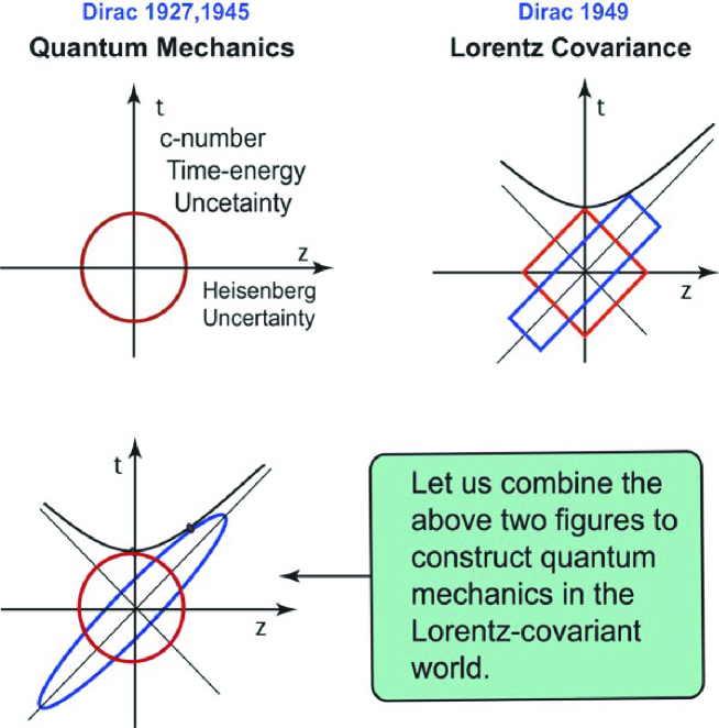
As we all know, quantum mechanics and special relativity were developed along two separate routes. As early as 1927, Dirac was interested in understanding whether these two scientific disciplines are compatible with each other. In his paper of 1927ย [4], Dirac noted the the existence of the time-energy uncertainty relation without excitations. He called this the โ€œc-numberโ€ time-energy uncertainty relation. Dirac pointed out that the space-time asymmetry makes it difficult to construct the uncertainty relation in the Lorentz-covariant world.

Refer to caption

Figure 4: Diracโ€™s three papers. His 1927 and 1945 papers can be described by a circle in the longitudinal space-like and time-like coordinate. Dirac introduced the light-cone coordinate system in 1959. In this system, the Lorentz boost is a squeeze transformation. It is then natural to synthesize these two figures to a squeezed circle or an ellipse. Figureย 6 will illustrate how this elliptic squeeze manifests itself in the real world.

In 1945, Dirac considered the four-dimensional harmonic oscillator wave functions applicable to the four-dimensional space and time. In so doing, Dirac was considering localized bound states. The space and time variables in his case are the separations between two constituents, like the proton and electron in the hydrogen atom.

It was shown later that Diracโ€™s concern about the c-number time-energy uncertainty is not necessary in view of the fact that a massive particle at rest has only three space-like dimensionsย [13]. According to Wignerย [14], the little group for the massive particle is isomorphic to $O(3)$ย [14]. With this understanding, we can use a circle in the $z~{}t$ plane as shown in Fig.ย 4, where $z$ and $t$ are longitudinal and time separations respectively.

In his 1949 paperย [15], Dirac introduced the light-cone coordinate system which tells us that the Lorentz boost is a squeeze transformation. This aspect is also illustrated in Fig.ย 4. It is then not difficult to see how the circle looks to a moving observer.

Refer to caption

Figure 5: The Bohr-Einstein issue is 100 years old. Fifty years later, it became the quark-parton puzzle, based on observations made in high-energy laboratories.

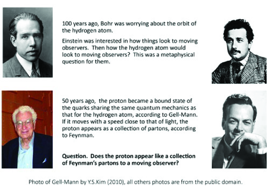
Next question is whether this elliptic squeeze has anything to do with the real world. One hundred years ago, Niels Bohr and Albert Einstein met occasionally to discuss physics. Their interests were different. Bohr was worrying about the electron orbit in the hydrogen atom. Einstein was interested in how things look to moving observers. Then the question arises. How would the hydrogen atom look to a moving observer? This was a metaphysical issue during the period of Bohr and Einstein, because there were no hydrogen atoms moving fast enough to exhibit this Einstein effect.

Fifty years later, the physics world was able to produce many protons from particle accelerators. In 1964ย [16], Gell-Mann observed that the proton is a bound state of the more fundamental particles called โ€œquarksโ€ according to the quantum mechanics applicable also to the hydrogen atom.
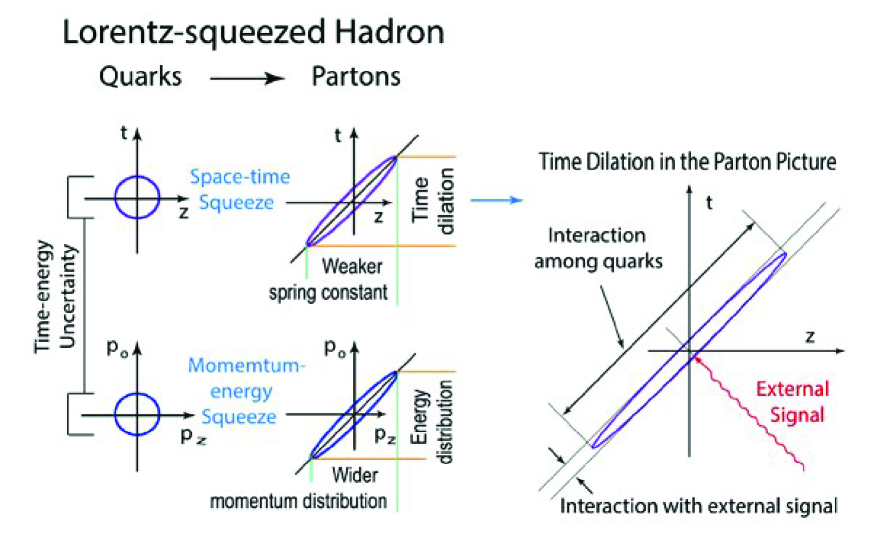
However, according to Feynmanย [17, 18], when the proton moves very fast, it appears as a collection of a large number of free-moving light-like partons with a wide-spread momentum distribution, as described in Fig.ย 6. Feynmanโ€™s parton picture was entirely based on what we observe in laboratories.

Unlike the hydrogen atom, the proton can become accelerated, and its speed could be very close to that of light. Thus the Bohr-Einstein issue became the Gell-Mann-Feynman issue, as illustrated in Fig.ย 5. The question is whether Gell-Mannโ€™s quark model and Feynmanโ€™s parton picture are two different aspects of one Lorentz-covariant entity. This question was addressed by Kim and Noz 1977ย [19] and was explained in detail by the present authors with a graphical illustration given in Fig.ย 6.

Refer to caption

Figure 6: In the harmonic-oscillator regime, the momentum-energy wave function takes the same mathematical form as that of the space-time wave functions. This figure shows that the quark model and the parton model are two different aspects of one Lorentz-covariant entity. In 1969ย [17], Feynman observed that the fast-moving proton appears as a collection of a large number of light-like partons with a wide-spread momentum distribution, and short interaction time with the external signal. This figure is a graphical illustration of the 1977 paper by Kim and Nozย [19]. This figure is from a recent book by the present authorsย [20].

References

  • [1] Dirac, P. A. M. Forms of Relativistic Dynamics. Rev. Mod. Phys. 1949 21, 392 - 399.
  • [2] Dirac, P. A. M. A Remarkable Representation of the 3 + 2 de Sitter Group. J. Math. Phys. 1963 4, 901 - 909.
  • [3] Inรถnรผ, E.; Wigner, E. P. On the Contraction of Groups and their Representations. Proc. Natl. Acad. Sci. (U.S.) 1953 39, 510 - 524.
  • [4] Dirac, P. A. M. The Quantum Theory of the Emission and Absorption of Radiation Proc. Roy. Soc. (London) 1927 A114 243 - 265.
  • [5] Han, D.; Kim, Y. S.; Noz, M.E. Linear canonical transformations of coherent and squeezed states in the Wigner phase space. Phys. Rev. A 1988 37, 807 - 814.
  • [6] Kim, Y. S.; Wigner, E. P. Canonical transformation in quantum mechanics. Am. J. Phys. 1990, 58, 439 - 447.
  • [7] Kim, Y. S.; Noz, M. E. Phase Space Picture of Quantum Mechanics; World Scientific Publishing Company: Singapore, 1991.
  • [8] Dodonov, V. V.; Manโ€™ko V. I. Theory of Nonclassical States of Light; Taylor & Francis: London & New York, 2003.
  • [9] Han, D.; Kim, Y. S.; Noz, M. E. $O(3,3)$-like Symmetries of Coupled Harmonic Oscillators. J. Math. Phys. 1995 36, 3940 - 3954.
  • [10] Abraham, R.; Marsden, J. E. Foundations of Mechanics 2nd ed. Benjamin Cummings: Reading, Massachusetts, 1978.
  • [11] Goldstein, H. Classical Mechanics. 2nd ed. Addison-Wesley: Reading, Massachusetts, 1980.
  • [12] BaลŸkal, S.; Kim, Y. S.; Noz, M. E. Poincarรฉ Symmetry from Heisenbergโ€™s Uncertainty Relations. Symmetry 2019 11, (3) 49:1 - 9.
  • [13] Kim, Y. S.; Noz, M. E.; Oh, S. H. Representations of the Poincarรฉ group for relativistic extended hadrons J. Math. Phys. 1979 20 1341 - 1344.
  • [14] Wigner, E. On unitary representations of the inhomogeneous Lorentz group Ann. Math. 1939, 40, 149 - 204.
  • [15] Dirac, P. A. M. Unitary Representations of the Lorentz Group Proc. Roy. Soc. (London) 1945 A183 284 - 295.
  • [16] Gell-Mann, M. A Schematic Model of Baryons and Mesons Phys. Lett. 1964 8, 214 - 215.
  • [17] Feynman, R. P. Very High-Energy Collisions of Hadrons Phys. Rev. Lett. 1969 23 1415 - 1417.
  • [18] Bjorken, J. D.; Paschos, E. A. Electron-Proton and $\gamma$-Proton Scattering and the Structure of the Nucleon Phys. Rev. 1969 185 1975 - 1982.
  • [19] Kim, Y. S.; Noz, M. E. Covariant harmonic oscillators and the parton picture Phys. Rev. D 1977 15 335 - 338.
  • [20] BaลŸkal, S; Kim. Y. S.; E. Noz, M. E. Physics of the Lorentz Group, IOP Concise Physics Morgan & Claypool Publisher, San Rafael, California, U.S.A. and IOP Publishing, Bristol, UK., 2015.