Meta Label Correction for Noisy Label Learning

Abstract

Leveraging weak or noisy supervision for building effective machine learning models has long been an important research problem. Its importance has further increased recently due to the growing need for large-scale datasets to train deep learning models. Weak or noisy supervision could originate from multiple sources including non-expert annotators or automatic labeling based on heuristics or user interaction signals. There is an extensive amount of previous work focusing on leveraging noisy labels. Most notably, recent work has shown impressive gains by using a meta-learned instance re-weighting approach where a meta-learning framework is used to assign instance weights to noisy labels. In this paper, we extend this approach via posing the problem as a label correction problem within a meta-learning framework. We view the label correction procedure as a meta-process and propose a new meta-learning based framework termed MLC (Meta Label Correction) for learning with noisy labels. Specifically, a label correction network is adopted as a meta-model to produce corrected labels for noisy labels while the main model is trained to leverage the corrected labels. Both models are jointly trained by solving a bi-level optimization problem. We run extensive experiments with different label noise levels and types on both image recognition and text classification tasks. We compare the re-weighing and correction approaches showing that the correction framing addresses some of the limitations of re-weighting. We also show that the proposed MLC approach outperforms previous methods in both image and language tasks.

Introduction

Recent advances in deep learning have enabled impressive performance on various tasks, including image recognition (He et al. 2016) and natural language processing (Devlin et al. 2018). At the core of this success lies the availability of large amounts of annotated data. However, such datasets are not readily available at scale for many tasks. Learning with weak supervision aims to address this challenge by leveraging weak evidences of supervision. Weak supervision can come in several forms including: incomplete supervision; where only a small subset of the training data has labels, inexact supervision; where only coarse-grained annotations are available, and inaccurate supervision; where noisy labels are given  (Zhou 2017). In this work, we focus on using inaccurate (noisy) labels as a form of weak supervision. Noisy labels may originate from multiple sources including: corrupted labels, non-expert annotators, automatic labels based on heuristics or user interaction signals, etc.

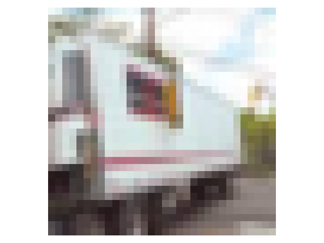
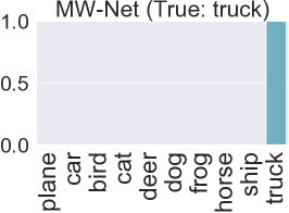
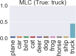
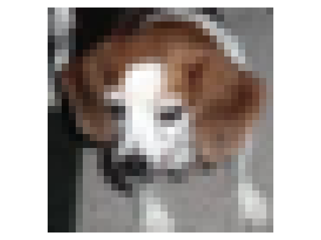
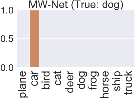
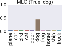
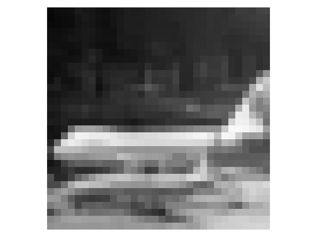
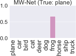
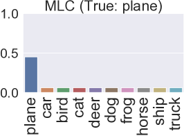
Figure 1: Illustration of label reweighting vs label correction. The first image is a truck and the given noisy label is truck, where MW-Net (A label reweighting method) and MLC successfully recover it. However, for the second image whose true label is dog and the given noisy label is automobile, MW-Net is unable to down-weight the incorrect label while MLC correctly adjusts its label by predicting the maximum weight on the class dog than all other classes. So is the case for the airplane with noisy label frog.

Training deep networks with noisy labels is challenging since they are prone to fitting and memorizing the noise (Zhang et al. 2017) given their high model capacity. As such, multiple lines of work have been proposed recently to effectively combine clean (or gold) labeled data with noisy (or weak) supervision data for more effective learning. One line of work focused on selecting samples from the noisy data that are likely to be correct using co-teaching or curriculum learning  (Jiang et al. 2017; Han et al. 2018b). Another line of work tries to re-weight the weak instances for selective training  (Ren et al. 2018; Shu et al. 2019), instead of either including or excluding them. Some of these approaches use a meta-learning framework to assign importance scores to each sample in the noisy training set such that the ones with higher weights can contribute more to the main model training  (Ren et al. 2018; Shu et al. 2019).

One of the limitations of label re-weighting is that it is limited to up or down weighting the contribution of an instance in the learning process. An alternative approach relies on the idea of label correction. It aims to correct the noisy labels based on certain assumptions about the weak label generation process. In a sense, label correction aims to go beyond selecting or assigning high weights to useful examples to also altering the assigned labels of incorrectly labeled examples. However, previous methods of label correction rely on assumptions about the weak label generation process and thus often involves two independent steps: (1) estimating a label corruption matrix (Hendrycks et al. 2018), (2) training a model on the noisy data leveraging the corruption matrix. Estimating the corruption matrix often involves assumptions about the noise generation process, such as assuming that the noisy label is only dependent on the true label and is independent of the data itself (Hendrycks et al. 2018).

In this paper, we adopt label correction to address the problem of learning with noisy labels, from a meta-learning perspective. We term our method meta label correction (MLC). Specifically, we view the label correction procedure as a meta-process, which objective is to provide corrected labels for the examples with noisy labels. Meanwhile, the main predictive model is trained with such corrected labels generated by the meta-model. Both the meta-model and the main model are learned concurrently via a bi-level optimization procedure. This allows the model to maximize the performance on the clean data set (i.e., the clean labels serve as a validation set w.r.t. the noisy set) by updating the label correction process in a differentiable manner. MLC extends work on re-weighting and correction leveraging the advantages of both approaches. In contrast to meta-learning based instance re-weighting, which only considers up or down weighting the given noisy label, MLC provides a more refined way of leveraging noisy labels by exploring all possible classes in the label space. In contrast to previous label correction methods, MLC doesn’t make assumptions about the underlying label noises and concurrently learns a correction model with the main model. Figure 1 shows examples where label re-weighting could at best down-weight noisy samples, reducing their impact on the learning process. On the other hand, MLC can successfully correct the noisy labels to the true ones.

Meta learning has been successfully used for many applications including hyper-parameter tuning (Maclaurin, Duvenaud, and Adams 2015), optimizer learning (Ravi and Larochelle 2017), model selection (Pedregosa 2016), adaptation to new tasks (Finn, Abbeel, and Levine 2017) and neural architecture search (Liu, Simonyan, and Yang 2019). This work leverages meta-learning for label correction to learn from noisy labels and makes the following contributions:

• We pose the problem of learning from weak (noisy) supervision as a meta label correction where a correction network is trained as a meta process to provide reliable labels for the main models to learn;

• We compare and contrast re-weighting and correction as two strategies for handling noisy labeled data;

• We conduct experiments on a combination of 3 image recognition and 4 large-scale text classification tasks with varying noise levels and types, including real-world noisy labels. We show that the proposed method outperform previous best methods on label correction and re-weighting, demonstrating the power of the proposed method.

Related Work

Labeled data largely determines whether a machine learning system can perform well on a task or not, as noisy label or corrupted labels could cause dramatic performance drop (Nettleton, Orriols-Puig, and Fornells 2010). The problem gets even worse when an adversarial rival intentionally injects noises into the labels (Reed et al. 2014). Thus, understanding, modeling, correcting, and learning with noisy labels has been of interest at large in the research communities (Natarajan et al. 2013; Frénay and Verleysen 2013). Several approaches  (Mnih and Hinton 2012; Patrini et al. 2017; Sukhbaatar et al. 2014; Larsen et al. 1998) have attempted to address the weak labels by modifying the model’s architecture or by implementing a loss correction.  (Sukhbaatar et al. 2014) introduced a stochastic variant to estimate label corruption, however the method has to have access to the true labels, rendering it inapplicable when no true labels are present. A forward loss correction adds a linear layer to the end of the model and the loss is adjusted accordingly to incorporate learning about the label noise.  (Patrini et al. 2017) also make use of the forward loss correction mechanism, and propose an estimate of the label corruption estimation matrix which relies on strong assumptions, and does not make use of clean labels that might be available for a portion of the data set. Similar idea is also explored in  (Goldberger and Ben-Reuven 2017).

In this paper, we limit our attention to the setting where in addition to a large amount of weakly labeled data, there is also a small set of clean data available. Under this setup, two major lines of work have been proposed to solve learning problem with noisy labels and we briefly review them here.

Learning with Label Correction

The first line of work aims to correct the weak labels as much as possible by imposing assumptions of how the noisy labels are generated from its underlying true labels. Consider the problem of classifying the data into $k$ categories, label correction involves estimating a label corruption matrix $C_{k\times k}$ whose entry $C_{ij}$ denotes the probability of observing noisy label for class $i$ while the underlying true class label is actually $j$ (Han et al. 2018a; Yao et al. 2020; Xia et al. 2019). For example, gold loss correction (Hendrycks et al. 2018) falls into this category; a key drawback of this line of work is that the label corruption matrix is estimated in an adhoc way and also that the estimation process is separate from the main model process, hence allowing no feedback from the main model to the estimation process. In addition, the estimated label corruption matrices are global, thus ignoring data dependent noises, a setting prevalent in real world label noises(Xia et al. 2020).

Learning to Re-weight Training Instances

Knowing that not all training examples are equally important and useful for building a main model given the noise, another line of work for learning with weak supervision focuses on selecting a subset of samples from the noisy data that are likely to be correct  (Jiang et al. 2017; Han et al. 2018b; Yu et al. 2019; Fang et al. 2020). Instead of discarding examples, an extension of this idea focused on assigning learnable weights to each example in the training noisy set. The goal is to assign a weight for each training example, indicating how useful the example is, such that the main model could use these weights to improve performance on a separate validation set (the clean set)  (Ren et al. 2018; Shu et al. 2019). The example weights are essentially hyper-parameters for the main model and can be learned by formulating a bi-level optimization problem. This framework allows the example weights learning and the main model to communicate with each other and a better model could be learned.

Our work follows the learning to correct framework by learning to model and correct the label noise in the noisy examples. Instead of separately handling the label correction and model learning steps, we propose a meta-learning approach to co-optimize for the two steps. We show that our model can outperform state-of-the-art methods for both learning to correct and learning to re-weight.

Meta Label Correction

Following (Charikar, Steinhardt, and Valiant 2017; Veit et al. 2017; Li et al. 2017; Xiao et al. 2015; Ren et al. 2018), we assume that the setup of learning with noisy labels involves two sets of data: a small set of data with clean/trusted labels and a large set of data with noisy/weak labels. Typically the clean set is much smaller compared to the noisy set, due to scarcity of expert labels and high labeling costs. Training directly on the small clean set often tends to be sub-optimal, as too little data can easily cause over-fitting. Training directly on the noisy set (or a combination of the noisy and clean sets) also tends to be sub-optimal, as large high-capacity models can fit and memorize the noise (Zhang et al. 2017). Note that unlike some of the work in this area, e.g., (Veit et al. 2017), we do not require having trusted and noisy labels for the same instances.

One advantage of the label correction approach is that it allows us to combine clean labels and corrected noisy labels in the learning process. Our proposed approach adopts the label correction methodology while also co-optimizing the label correction process together with the main model process through a unified meta-learning framework. We achieve that by training a meta learner (meta model) that tries to correct the noisy labels and a main model that tries to build the best predictive model with corrected labels coming from the meta model, allowing the meta model and main model to reinforce each other.

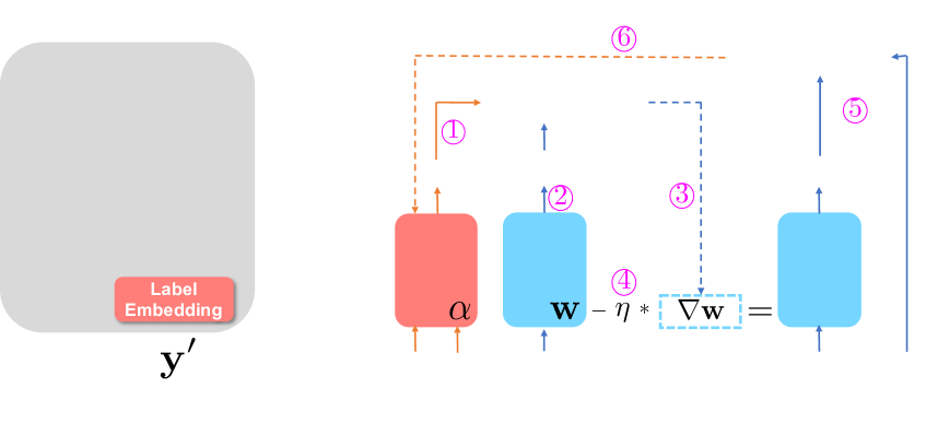
Figure 2: MLC computation graph. $(\bm{\mathbf{x}}_{i},\bm{\mathbf{y}}_{i}^{\prime})$ denotes a pair of sample with weak label and $(\bm{\mathbf{x}}_{j},\bm{\mathbf{y}}_{j})$ is a pair of sample with clean label. (a) Architecture of the label correction network, where $h(\bm{\mathbf{x}})$ is a feature representation of input $\bm{\mathbf{x}}$; (b) Computation flow of updating the LCN. In order, operations are: ① Feed the weak instance to the LCN and get its corrected label, ② Feed the data instance to the current classifier and compute the logits for prediction, ③ Compute the loss with the logits and corrected label, and compute the gradient of the loss w.r.t. the parameter of the classifier. Note that the gradient will be a function of the parameters of the LCN. ④ Update the classifier parameter while keeping the computation graph for its gradient, ⑤ Feed a pair of clean instance to the new model and compute its loss, ⑥ Compute the gradient of the loss w.r.t the parameter of LCN and update the LCN.

A Meta-learning Method for Label Correction

We describe the framework in detail as follows. Given a set of clean data examples $D=\{\bm{\mathbf{x}},\bm{\mathbf{y}}\}^{m}$ and a set of weak (noisy) data examples $D^{\prime}=\{\bm{\mathbf{x}},\bm{\mathbf{y}}^{\prime}\}^{M}$ with $m$ much smaller than $M$. To best exploit the information carried by the weak labels, we propose to construct a label correction network (LCN), serving as a meta model, which takes a pair of noisy data example and its weak label as input and attempts to produce a corrected label for this data example. The LCN is parameterized as a function with parameters $\bm{\mathbf{\alpha}}$, $y_{c}=g_{\bm{\mathbf{\alpha}}}(h(\bm{\mathbf{x}}),y^{\prime})$ to correct the weak label $y^{\prime}$ of example feature $h(\bm{\mathbf{x}})$ to a more accurate one. (Note that $y_{c}$ is a soft label, i.e., a multinomial distribution for all possible classes and the subscription in $y_{c}$ emphasizes that it’s generating a corrected label). Meanwhile, the main model $f$, that we aim to train and use for prediction after training, is instantiated as another function with parameters $\bm{\mathbf{w}}$, $y=f_{\bm{\mathbf{w}}}(\bm{\mathbf{x}})$.

Without linking the two models, there’s no way to enforce that: 1) the corrected label from LCN for an example from the meta model $g$ is indeed a meaningful one, let alone a corrected one, since directly training the LCN is not possible without clean labels for the noisy examples ; 2) The main model $f$ ends up fitting onto the correct true labels, if the labels provided by the LCN do not align with the unknown true labels. Fortunately, the two models can be linked together via a bi-level optimization framework, motivated by the intuition that if the labels generated by the LCN are of high quality, then a classifier trained with such corrected labels as supervision should achieve low loss on a separate set of clean examples. Formally, this can be formulated as the following bi-level optimization problem:

$$\min_{\bm{\mathbf{\alpha}}}\,\mathbb{E}_{(\bm{\mathbf{x}},y)\in D}\,\ell\left(y,f_{\bm{\mathbf{w}}^{*}_{\bm{\mathbf{\alpha}}}}(\bm{\mathbf{x}})\right)$$ (1)

$$\,\,\,\,\mbox{s.t. }\,\,\bm{\mathbf{w}}^{*}_{\bm{\mathbf{\alpha}}}=\arg\min_{\bm{\mathbf{w}}}\mathbb{E}_{(\bm{\mathbf{x}},y^{\prime})\in D^{\prime}}\,\ell\left(g_{\bm{\mathbf{\alpha}}}(h(\bm{\mathbf{x}}),y^{\prime}),f_{\bm{\mathbf{w}}}(\bm{\mathbf{x}})\right)$$

where $\ell(\cdot)$ is the loss function for classification, i.e., cross-entropy. We term this framework as Meta Label Correction (MLC); Figure 2 provides an overview of the framework. Note that to facilitate a light-weight design of the LCN, we take $h(\bm{\mathbf{x}})$ to be the feature representations from the main classifier, e.g., representations from the last layer, with stop-gradient operators before feeding to LCN to prevent gradient flowing the LCN back to the main model.

In this bi-level optimization, the LCN parameters $\bm{\mathbf{\alpha}}$ are the upper parameters (or meta parameters) while the main model parameters $\bm{\mathbf{w}}$ are the lower parameters (or main parameters). Like many other work involving bi-level optimizations, exact solutions to Problem (1) requires solving for the optimal $\bm{\mathbf{w}}^{*}$ whenever $\bm{\mathbf{\alpha}}$ gets updated. This is both analytically infeasible and computationally expensive, particularly when the main model $f$ is complex, such as ResNet (He et al. 2016) for image recognition and BERT (Devlin et al. 2018) for text classification.

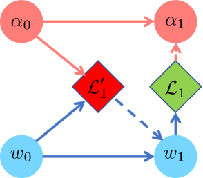
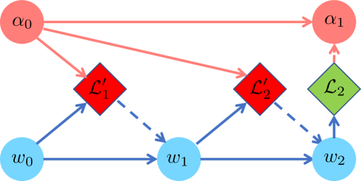
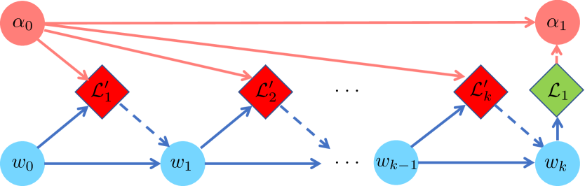
Figure 3: Different bi-level optimization learning strategies. (a) For any step, the optimal $\bm{\mathbf{w}}^{*}_{\bm{\mathbf{\alpha}}}$ is approximated with one-step look-ahead optimizer update, and used to compute the evaluation loss $\mathcal{L}_{1}$, which is then used to update $\bm{\mathbf{\alpha}}$. (b) $\bm{\mathbf{\alpha}}$ are updated once every two updates from $\bm{\mathbf{w}}$, i.e., a two-step look-ahead update is used to approximate $\bm{\mathbf{w}}^{*}_{\bm{\mathbf{\alpha}}}$. (c) Extending to $k$-step look-ahead approximation of $\bm{\mathbf{w}}^{*}_{\bm{\mathbf{\alpha}}}$ for updating $\bm{\mathbf{\alpha}}$. We find using a $k$ in the range of $1\sim 10$ works well empirically.

Gradient-based optimization for bi-level optimization. Outside of label correction research, various other studies, including differentiable architecture search (Liu, Simonyan, and Yang 2019), few-shot meta learning (Finn, Abbeel, and Levine 2017; Nichol, Achiam, and Schulman 2018), have used similar bi-level formulation as Problem (1). Instead of solving for the optimal for $\bm{\mathbf{w}}^{*}$ for each $\bm{\mathbf{\alpha}}$, one step of SGD update for $\bm{\mathbf{w}}$ to approximate the optimal main model for a given $\bm{\mathbf{\alpha}}$ has been employed

$$\bm{\mathbf{w}}^{*}_{\bm{\mathbf{\alpha}}}\approx\bm{\mathbf{w}}^{\prime}(\bm{\mathbf{\alpha}})=\bm{\mathbf{w}}-\eta\nabla_{\bm{\mathbf{w}}}\mathcal{L}_{D^{\prime}}(\bm{\mathbf{\alpha}},\bm{\mathbf{w}})$$ (2)

where $\mathcal{L}_{D^{\prime}}(\bm{\mathbf{\alpha}},\bm{\mathbf{w}})\triangleq\mathbb{E}_{(\bm{\mathbf{x}},y^{\prime})\in D^{\prime}}\,\ell\left(g_{\bm{\mathbf{\alpha}}}(\bm{\mathbf{x}},y^{\prime}),f_{\bm{\mathbf{w}}}(\bm{\mathbf{x}})\right)$ is a shorthand for the lower-level objective function and $\eta$ is the learning rate for the main model $f$. Denoting the upper-level objective function (meta loss) as $\mathcal{L}_{D}(\bm{\mathbf{w}})\triangleq\bm{\mathbf{w}}$ $\mathbb{E}_{(\bm{\mathbf{x}},y)\in D}\,\ell(y,f_{\bm{\mathbf{w}}}(\bm{\mathbf{x}}))$, the proxy optimization problem with one-step look ahead SGD now becomes

$$\min_{\bm{\mathbf{\alpha}}}\,\mathcal{L}_{D}(\bm{\mathbf{w}}^{\prime}(\bm{\mathbf{\alpha}})) =\mathcal{L}_{D}(\bm{\mathbf{w}}-\eta\nabla_{\bm{\mathbf{w}}}\mathcal{L}_{D^{\prime}}(\bm{\mathbf{\alpha}},\bm{\mathbf{w}}))$$ (3)

Efficient Meta-gradient with $k$-step SGD of Main Parameters

Different from DARTS (Liu, Simonyan, and Yang 2019), the meta loss $\mathcal{L}_{D}(\bm{\mathbf{w}}^{*}_{\bm{\mathbf{\alpha}}})$ depends only implicitly on the meta parameters $\bm{\mathbf{\alpha}}$ via the trained model $\bm{\mathbf{w}}^{*}_{\bm{\mathbf{\alpha}}}$, hence a more accurate estimate of the optimal solution $\bm{\mathbf{w}}^{*}_{\bm{\mathbf{\alpha}}}$ for the current LCN parameters $\bm{\mathbf{\alpha}}$ is desired. To this end, we propose to employ a $k$-step ahead SGD update as the proxy estimate for the optimal solution. Figure 3 demonstrates the parameter updating schemes for different $k$. A larger $k$ principally provides less noisy estimate for the optimal solution $\bm{\mathbf{w}}^{*}_{\bm{\mathbf{\alpha}}}$, however it also results in longer dependencies over the past $k$ iterations, which requires caching $k$ copies of the model parameters $\bm{\mathbf{w}}$. To address this, we further propose to approximate the current meta-parameter gradient with information from the previous $k$ step as follows

$$\frac{\partial\bm{\mathbf{w}}^{\prime}}{\partial\bm{\mathbf{\alpha}}} =\left(I-\Lambda H_{\bm{\mathbf{w}},\bm{\mathbf{w}}}\right)\frac{\partial\bm{\mathbf{w}}}{\partial\bm{\mathbf{\alpha}}}-\Lambda H_{\bm{\mathbf{\alpha}},\bm{\mathbf{w}}}$$ (4)

$$g_{\bm{\mathbf{w}}^{\prime}}\frac{\partial\bm{\mathbf{w}}^{\prime}}{\partial\bm{\mathbf{\alpha}}} =g_{\bm{\mathbf{w}}^{\prime}}\left(I-\Lambda H_{\bm{\mathbf{w}},\bm{\mathbf{w}}}\right)\frac{\partial\bm{\mathbf{w}}}{\partial\bm{\mathbf{\alpha}}}-g_{\bm{\mathbf{w}}^{\prime}}\Lambda H_{\bm{\mathbf{\alpha}},\bm{\mathbf{w}}}$$ (5)

$$\frac{\partial\mathcal{L}_{D}(\bm{\mathbf{w}}^{\prime})}{\partial\bm{\mathbf{\alpha}}} \approx g_{\bm{\mathbf{w}}^{\prime}}\left(I-\Lambda\right)\frac{g_{\bm{\mathbf{w}}^{\top}}}{\|g_{\bm{\mathbf{w}}}\|^{2}}\frac{\partial\mathcal{L}_{D}(\bm{\mathbf{w}})}{\partial\bm{\mathbf{\alpha}}}-g_{\bm{\mathbf{w}}^{\prime}}\Lambda H_{\bm{\mathbf{\alpha}},\bm{\mathbf{w}}}$$ (6)

where $\bm{\mathbf{w}}^{\prime}$ is the model parameter for next step, $g_{\bm{\mathbf{w}}}$ is a short hand for the gradient of the training loss w.r.t $\bm{\mathbf{w}}$, $\Lambda$ is a diagonal matrix representing the current learning rates for all parameters in $\bm{\mathbf{w}}$, and $H_{\bm{\mathbf{\alpha}},\bm{\mathbf{w}}}$ is a short hand for $\frac{\partial^{2}}{\partial\bm{\mathbf{\alpha}}\partial\bm{\mathbf{w}}}\mathcal{L}_{D^{\prime}}(\bm{\mathbf{\alpha}},\bm{\mathbf{w}})$. $H_{\bm{\mathbf{w}},\bm{\mathbf{w}}}$ is estimated with identity to ease computation and the second term can be computed as

$$g_{\bm{\mathbf{w}}^{\prime}}\Lambda H_{\bm{\mathbf{\alpha}},\bm{\mathbf{w}}}= \nabla_{\bm{\mathbf{\alpha}},\bm{\mathbf{w}}}^{2}\mathcal{L}_{D^{\prime}}(\bm{\mathbf{\alpha}},\bm{\mathbf{w}})\Lambda\nabla_{\bm{\mathbf{w}}^{\prime}}\mathcal{L}_{D}(\bm{\mathbf{w}}^{\prime})$$

$$= \nabla_{\bm{\mathbf{\alpha}}}\Big{(}\nabla_{\bm{\mathbf{w}}}^{\top}\mathcal{L}_{D^{\prime}}(\bm{\mathbf{\alpha}},\bm{\mathbf{w}})\Lambda\nabla_{\bm{\mathbf{w}}^{\prime}}\mathcal{L}_{D}(\bm{\mathbf{w}}^{\prime})\Big{)}$$ (7)

Algorithm 1 outlines an iterative procedure to solve the above proxy problem with $k$-step look ahead SGD for the main model.

while not converged do

       Update meta parameters $\bm{\mathbf{\alpha}}$ by descending Eq. (6)

      Update model parameters $\bm{\mathbf{w}}$ by descending $\nabla_{\bm{\mathbf{w}}}\mathcal{L}_{D^{\prime}}(\bm{\mathbf{\alpha}},\bm{\mathbf{w}})$

end while

Algorithm 1 MLC - Meta Label Correction

Training with Soft Labels from LCN

Not only does the LCN explicitly model the dependency of the corrected label on both the data example and its noisy label, but also it ensures that the output from the LCN is a valid categorical distribution over all possible classes. Soft labels are crucial in MLC as they make gradient propagation back to the meta model from the main model possible. However, when the main model takes these examples with soft corrected labels, it brings difficulty to training due to the additional uncertainly in the corrected labels. This can be alleviated by the following strategy. In training for each batch of clean data, we split it into two parts, with one serving as the clean evaluation set and add the other to the training process for $f$, as a small portion of the clean set will provide clean guidance for training, to ease model training. This has been shown to be effective in similar settings (Ranzato et al. 2015; Pham et al. 2020).

Remark: Label Correction vs Label Reweighting

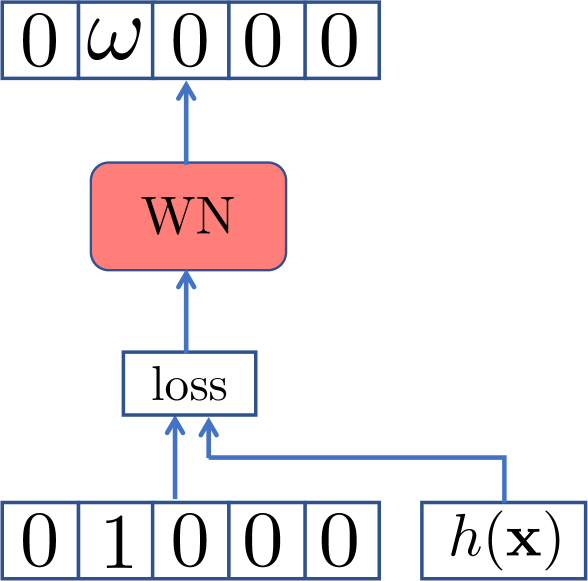
(a) Weighting-Network (WN) in Meta-WN (Shu et al. 2019)

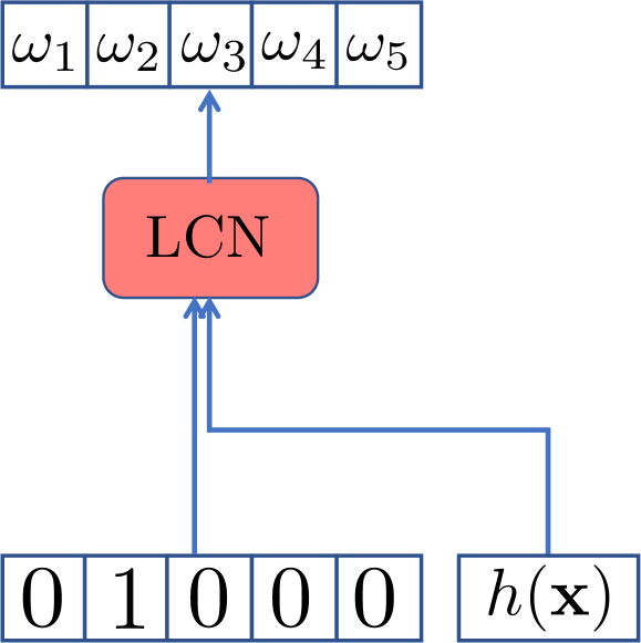
(b) Label Correction Network (LCN) in MLC (Ours)

Figure 4: Different treatments of noisy labels from Meta-WN and MLC. Total number of classes assumed to be 5 for illustration purpose. (a) Meta-WN; (b) MLC.

To address noisy labels, Meta-WN (Shu et al. 2019) leverages the Weight-Network (WN) as the meta-module to reweight the given noisy label, while MLC aims to provide a more refined treatment, i.e., to correct the noisy label. More explicitly, Figure 4 demonstrates the difference of the underlying operations between Meta-WN and MLC. To highlight

• For an input, Meta-WN tries to learn a weight for the given noisy class only, whiling ignoring all other possible classes (demonstrated by the single non-negative weight $\omega$ for Class 2 while $0$ for all other classes in Figure 4(a)), while since MLC tries to correct the given weak label, essentially it considers all possible classes (demonstrated by the full non-negative vector resulting from the final softmax layer of the LCN, i.e., $(\omega_{1},\omega_{1},\omega_{3},\omega_{4},\omega_{5})$ for all classes with $\omega_{1}+\omega_{1}+\omega_{3}+\omega_{4}+\omega_{5}=1$, essentially weighting all possible classes)

• Another key difference between MLC and Meta-WN relies on the information bottleneck to their corresponding meta-modules. For Meta-WN doesn’t directly take an pair of data and noisy label as input, but rather relies on the scalar loss of the classifier that particular input incurs as input. In other words, the meta-module lacks the ability to differentiate the different input pairs if the loss values for them are similar, effectively limiting the modeling capacity of the meta-module. While the LCN in MLC directly takes the data feature $h(\bm{\mathbf{x}})$ and its weak label as input, allowing a more flexible treatment and enabling the LCN to identify different information brought by different input pairs.

Experiments

To test the performance of MLC, we conduct experiments on a combination of three image recognition and four text classification tasks, and compare with previous state-of-the-art approaches for learning with noisy labels under different types of label noises.

Datasets and Setup

Datasets. We evaluate our method on 3 image recognition datasets, CIFAR-10, CIFAR-100 (Krizhevsky 2009) and Clothing1M (Xiao et al. 2015) and 4 large-scale multi-class text classification benchmark datasets, that are widely used by text classification research (Zhang, Zhao, and LeCun 2015; Xie et al. 2019; Dai et al. 2019; Yang et al. 2016; Conneau et al. 2016), AG news, Amazon reviews, Yelp reviews and Yahoo answers. Information about all datasets is summarized in Table 1.

Dataset	CIFAR-10	CIFAR-100	Clothing1M	AG	Amazon-5	Yelp-5	Yahoo
# classes	10	100	14	4	5	5	10
Train	50K	50K	1.05M	120K	3M	650K	1.4M
Test	10K	10K	10K	7.6K	650K	50K	60K
Clean	1000	1000	50K	400	500	500	1000
Noisy	49K	49K	1M	119.6K	$\sim$ 3M	649.5K	$\sim$ 1.4M
Classifier	ResNet 32		ResNet 50	Pre-trained BERT-base

Table 1: Dataset statistics and classifier architectures used. Note the clean set is significantly smaller than the noisy label set.

Datasets	CIFAR-10	CIFAR-100	AG	Yelp-5	Amazon-5	Yahoo
($\#$ clean labels)	($10\times 100$)	($100\times 10$)	($4\times 100$)	($5\times 100$)	($5\times 100$)	($10\times 100$)
MW-Net (Shu et al. 2019)	65.12	39.96	75.91	51.27	49.49	60.18
GLC (Hendrycks et al. 2018)	86.62	50.50	83.88	60.12	60.31	68.03
MLC (Ours)	86.81	53.68	85.27	62.61	61.21	73.72

Table 2: Mean accuracies on all data sets. Each cell represents the average runs over two noise types and 10 noise levels. A $k=5$ (5-step ahead SGD) is used for all experiment. (Each configuration is run for 5 times and the mean is reported)

Method	Forward	Joint Learning	MLNT	MW-Net	GLC	MLC
	(Patrini et al. 2017)	(Tanaka et al. 2018)	(Li et al. 2019)	(Shu et al. 2019)	(Hendrycks et al. 2018)	(Ours)
Accuracy	69.84	72.23	73.47	73.72	73.69	75.78

Table 3: Test set accuracies on Clothing1M with real-world noisy labels ($k=5$)

Noisy label sources Following related work (Hendrycks et al. 2018; Ren et al. 2018; Shu et al. 2019), for each dataset, we sample a portion of the entire training set as the clean set (except for Clothing1M). To ensure a fair and consistent evaluation, we use only 1000 images as clean set for both CIFAR-10 and CIFAR-100, and only 100 instances per class for the four large scale text classification data sets. The noisy sets are generated by corrupting the labels of all the remaining data points based on the following two setting:

Uniform label noise (UNIF). For a dataset with $C$ classes, a clean example with true label $y$ is randomly corrupted to all possible classes $y^{\prime}$ with probability $\frac{\rho}{C}$ and stays in its original label with probability $1-\rho$. (Note the corrupted label might also happen to be the original label, hence the label has probability of $1-\rho+\frac{\rho}{C}$ to stay uncorrupted.)

Flipped label noise (FLIP). For a dataset with $C$ classes, a clean example with true label $y$ is randomly flipped to one of the rest $C-1$ classes with probability $\rho$ and stays in its original label with probability $1-\rho$.

We vary $\rho$ in the range of $[0,1]$ to simulate different noise levels for both types. We emphasize that both simulated noise types make the assumption that given the true label the noisy label doesn’t depend on the data itself. Hence we also evaluate all the methods on another source of noisy labels:

Real-world noisy labels. Clothing1M (Xiao et al. 2015) is a dataset where noisy labels for images are devised by leveraging user tags as proxy annotations. As Clothing1M is the only dataset that comes with real-world noisy labels, we use its original split of clean and noisy sets.

Finally, we also note that regardless of noise types, none of the methods tested in this paper is aware of the label corruption probability $\rho$ nor do they have knowledge about which data sample in the noisy set is actually corrupted.

Baseline Methods and Model Architectures

We focus our evaluation of MLC against state-of-the-art methods for learning with weak supervision from two different themes, i.e.,  (Hendrycks et al. 2018) for label correction (denoted by GLC hereafter) and instance re-weighting with meta learning  (Shu et al. 2019) (denoted by MW-Net hereafter). Note that GLC and MW-Net were shown to consistently outperform other methods such as training on clean data only, cleaning on weak data only, combining clean and weak data, as well as more sophisticated models for combining the clean and weak labels such as distillation (Li et al. 2017) and forward loss correction (Sukhbaatar et al. 2014). Additionally, MW-Net was shown to outperform a slightly different variant for instance re-weighting with meta-parameters (Ren et al. 2018). As such, we do not show results from these methods.

For fair and consistent comparisons, we use the same classifier architectures for all methods, i.e., ResNet 32 for CIFAR-10 and CIFAR-100, ResNet 50 pretrained from ImageNet for Clothing1M, and pre-trained BERT-base for the four large-scale text data sets. We implement all models and experiments in PyTorch. All models are trained with the same number of epochs for the same dataset.

LCN architecture. We use the same LCN architecture for MLC across all settings as follows (Figure 2(a)):

• An embedding layer of size $(C,128)$ to embed the input noisy labels, followed by a three-layer feed-forward network with dimensions of (128+xdim, hdim), (hdim, hdim), (hdim,C) respectively. tanh is used as the nonlinear activation function in-between them and lastly a Softmax layer to output a categorical distribution as the corrected labels

where $C$ is the number of classes, xdim is the feature dimension of input $\bm{\mathbf{x}}$ from the last layer from the main classifier, i.e., 64 from ResNet32 for CIFAR-10 and CIFAR-100, 2048 from ResNet 50 for Clothing1M and 768 from BERT-base for text datasets and hdim is the hidden dimension for the LCN (set to 768 for text datasets and 64 otherwise).

Main Results

MLC on image recognition. We start by comparing all methods on the standard image recognition datasets. Table 2 presents the averaged accuracies across multiple configurations (two noise types, 10 noise levels) with $k=5$. The table shows that MLC consistently outperforms other methods over all datasets. In addition, on Clothing1M with real noisy labels (Table 3), MLC outperforms all baseline methods and improves over GLC and MW-Net by over 2 points in accuracy, suggesting its ability to capture better data-dependent label corruptions via the meta-learning framework.

MLC on text classification. Table 2 also presents the mean accuracies of MLC on 4 large text data sets with pre-trained BERT-base as its main classifier. Overall, label reweighting (MW-Net) seems insufficient to fully address the text classification problem; label correction approaches demonstrate much higher performances, while MLC achieves the best thanks to its nature of combining of both label correction and the data-driven meta-learning framework.

Analysis and Ablation Studies

Effects of noise levels $\rho$ and $k$ for MLC. Figure 5 presents the results of all methods under UNIF with noise levels from 0 to 1.0 with a step size of 0.1. It’s clear that, since Meta-WN only attempts to re-weight the observed weak label, its performance decreases significantly when the noise level goes up, as the given label turns more likely to be the wrong label thus re-weighting for this case is insufficient; while label correction based methods (GLC and MLC) show to be robust against severe label noises. This is consistent with results reported in  (Hendrycks et al. 2018) where label correction was shown to perform well even in extreme noise level situations.

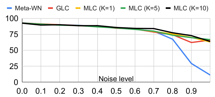
Figure 5: Test accuracy w.r.t noise levels

Moreover, we observe that MLC is more effective in doing this than previous label correction methods for severe noise. In terms of the number of look-ahead steps, $k$, used to compute the meta-gradient, the value of $k$ does not seem to have an impact on MLC’s performance when the noise level is low; however when the noise level is high (more than 0.6), a larger $k$ leads to higher test accuracy, validating the strategy of using multiple steps to compute the meta-gradients. Similar trends are also observed on FLIP.

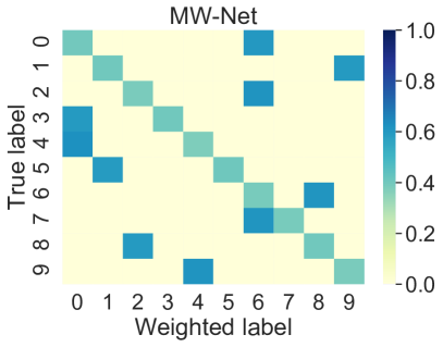
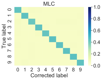
Figure 6: (a) Heatmap of learned weights of MW-Net w.r.t to the true labels; note that MW-Net does not alter the noisy labels but only assigns them weight. (b) Heatmap of probability distribution of the corrected labels of MLC w.r.t to the true labels; note that MLC can alter the input label (For all examples in the test set with noise level $\rho=0.6$.)

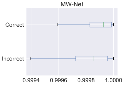
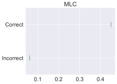
Figure 7: Effect of reweighting vs correction for FLIP with $\rho=0.6$. (Left) Weights assigned by MW-Net w.r.t to the input noisy label; (Right) Correction probabilities learned by LCN to the input noisy label.

Meta net evaluation. We perform additional experiments to understand what the meta model, i.e., the LCN, actually learns after model convergence. Additionally, we seek to quantify the benefit of correcting noisy labels, v.s. re-weighting instances. We use the FLIP setting to generate corrupted labels for instances in the test set in CIFAR-10 and feed them to the meta nets of both MLC and Meta-WN. MLC will produce a probability distribution over all possible classes where Meta-WN will assign a scalar weight to each instance. Note that, for CIFAR-10, we know which of the noisy label is actually correct and which is not but neither of the models have access to this information. Ideally, Meta-WN will assign higher weights to the correct instances and lower weights to the incorrect ones. Similarly, MLC should keep the label of correct instances as is and alter the labels of the incorrect ones. We see from Figure 7 that this is actually the case. On average, both model seem to be able to distinguish between the correct and incorrect labels. However, for incorrect labels, Meta-WN can only down-weight the sample reducing the dependence of the training process on it. MLC goes beyond this by also trying to change the label to assign the sample to the correct one, allowing the main model to fully leverage it. We can see from Figure 6 that it does that successfully. On other other hand, MW-Net can only assign a weight to the noisy label.

MLC training dynamics. Figure 8(a,b,c) shows the training progress for one run on the CIFAR-10 with UNIF under different noise levels. We monitor a set of different metrics during training, including the loss function on the noisy data with corrected labels, loss function on clean data, and the test set accuracy as training progresses. The figure shows that both losses decrease and test accuracy increases as the training process progresses. Note that with larger noise levels (hence more difficult cases), training with MLC gets harder (as seen by the slightly higher loss on clean data and loss on noisy data). However, MLC still converges and achieves good results on test set as shown in Figure 8(c).

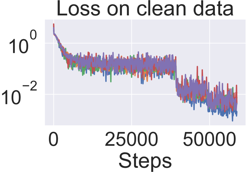
(a)

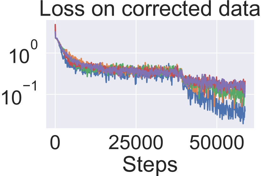
(b)

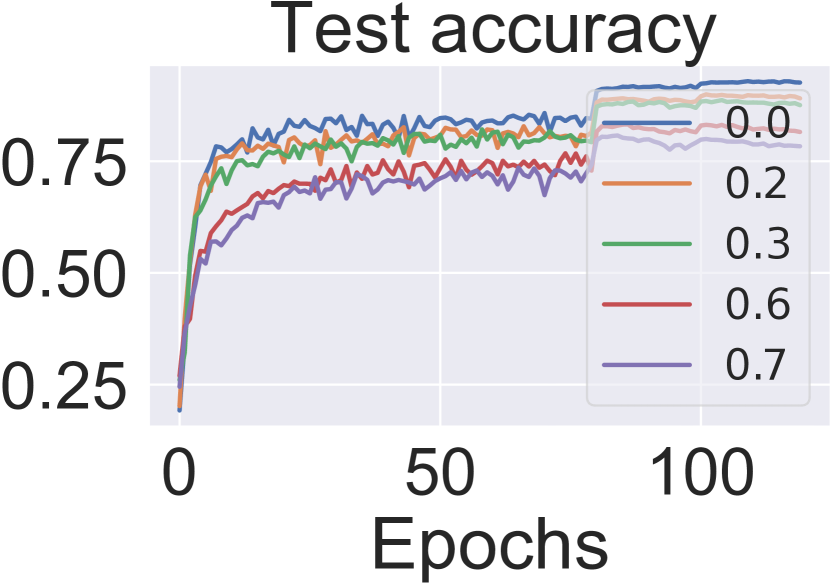
(c)

Figure 8: (a,b,c) Loss and test set accuracy dynamics w.r.t noise levels (losses are in log-scale). The two jump-points in the curves are due to the decay of learning rates at 60th and 80th Epoch, or $\sim$ 40K and 50K steps equivalently.

Conclusions

In this paper, we address the problem of learning with noisy labels from a meta-learning perspective. Specifically, we propose to use a meta network to correct the noisy labels from the data set, and a main classifier network is trained to fit the example to a provided label, i.e., corrected labels for the noisy examples and true labels for the clean ones. The meta network and main network are jointly optimized in a bi-level optimization fashion; to address the computation challenge, we employ a $k$-step ahead SGD update to compute the meta-gradient. Empirical experiments on three image recognition and four text classification tasks with various label noise types show the benefits of label correction over instance re-weighting and demonstrate the strong performance of MLC over previous methods leveraging noisy labels.

References

- Charikar, Steinhardt, and Valiant (2017) Charikar, M.; Steinhardt, J.; and Valiant, G. 2017. Learning from untrusted data. In Proceedings of the 49th Annual ACM SIGACT Symposium on Theory of Computing, 47–60. ACM.
- Conneau et al. (2016) Conneau, A.; Schwenk, H.; Barrault, L.; and Lecun, Y. 2016. Very deep convolutional networks for text classification. arXiv preprint arXiv:1606.01781 .
- Dai et al. (2019) Dai, Z.; Yang, Z.; Yang, Y.; Carbonell, J.; Le, Q. V.; and Salakhutdinov, R. 2019. Transformer-xl: Attentive language models beyond a fixed-length context. arXiv preprint arXiv:1901.02860 .
- Devlin et al. (2018) Devlin, J.; Chang, M.-W.; Lee, K.; and Toutanova, K. 2018. Bert: Pre-training of deep bidirectional transformers for language understanding. arXiv preprint arXiv:1810.04805 .
- Fang et al. (2020) Fang, T.; Lu, N.; Niu, G.; and Sugiyama, M. 2020. Rethinking Importance Weighting for Deep Learning under Distribution Shift. Advances in Neural Information Processing Systems 33.
- Finn, Abbeel, and Levine (2017) Finn, C.; Abbeel, P.; and Levine, S. 2017. Model-agnostic meta-learning for fast adaptation of deep networks. In Proceedings of the 34th International Conference on Machine Learning-Volume 70, 1126–1135. JMLR. org.
- Frénay and Verleysen (2013) Frénay, B.; and Verleysen, M. 2013. Classification in the presence of label noise: a survey. IEEE transactions on neural networks and learning systems 25(5): 845–869.
- Goldberger and Ben-Reuven (2017) Goldberger, J.; and Ben-Reuven, E. 2017. Training deep neural-networks using a noise adaptation layer. In 5th International Conference on Learning Representations, ICLR 2017, Toulon, France, April 24-26, 2017, Conference Track Proceedings. OpenReview.net.
- Han et al. (2018a) Han, B.; Yao, J.; Niu, G.; Zhou, M.; Tsang, I.; Zhang, Y.; and Sugiyama, M. 2018a. Masking: A new perspective of noisy supervision. Advances in Neural Information Processing Systems 31: 5836–5846.
- Han et al. (2018b) Han, B.; Yao, Q.; Yu, X.; Niu, G.; Xu, M.; Hu, W.; Tsang, I.; and Sugiyama, M. 2018b. Co-teaching: Robust training of deep neural networks with extremely noisy labels. In Advances in neural information processing systems, 8527–8537.
- He et al. (2016) He, K.; Zhang, X.; Ren, S.; and Sun, J. 2016. Deep residual learning for image recognition. In Proceedings of the IEEE conference on computer vision and pattern recognition, 770–778.
- Hendrycks et al. (2018) Hendrycks, D.; Mazeika, M.; Wilson, D.; and Gimpel, K. 2018. Using trusted data to train deep networks on labels corrupted by severe noise. In Advances in Neural Information Processing Systems, 10477–10486.
- Jiang et al. (2017) Jiang, L.; Zhou, Z.; Leung, T.; Li, L.-J.; and Fei-Fei, L. 2017. Mentornet: Learning data-driven curriculum for very deep neural networks on corrupted labels. arXiv preprint arXiv:1712.05055 .
- Kingma and Ba (2014) Kingma, D. P.; and Ba, J. 2014. Adam: A method for stochastic optimization. arXiv preprint arXiv:1412.6980 .
- Krizhevsky (2009) Krizhevsky, A. 2009. Learning multiple layers of features from tiny images. Master’s thesis, Department of Computer Science, University of Toronto .
- Larsen et al. (1998) Larsen, J.; Nonboe, L.; Hintz-Madsen, M.; and Hansen, L. K. 1998. Design of robust neural network classifiers. In Proceedings of the 1998 IEEE International Conference on Acoustics, Speech and Signal Processing, ICASSP’98 (Cat. No. 98CH36181), volume 2, 1205–1208. IEEE.
- Li et al. (2019) Li, J.; Wong, Y.; Zhao, Q.; and Kankanhalli, M. S. 2019. Learning to learn from noisy labeled data. In Proceedings of the IEEE Conference on Computer Vision and Pattern Recognition, 5051–5059.
- Li et al. (2017) Li, Y.; Yang, J.; Song, Y.; Cao, L.; Luo, J.; and Li, L.-J. 2017. Learning From Noisy Labels With Distillation. In The IEEE International Conference on Computer Vision (ICCV).
- Liu, Simonyan, and Yang (2019) Liu, H.; Simonyan, K.; and Yang, Y. 2019. DARTS: Differentiable Architecture Search. In 7th International Conference on Learning Representations, ICLR 2019, New Orleans, LA, USA, May 6-9, 2019. OpenReview.net.
- Maclaurin, Duvenaud, and Adams (2015) Maclaurin, D.; Duvenaud, D.; and Adams, R. 2015. Gradient-based hyperparameter optimization through reversible learning. In International Conference on Machine Learning, 2113–2122.
- Mnih and Hinton (2012) Mnih, V.; and Hinton, G. E. 2012. Learning to label aerial images from noisy data. In Proceedings of the 29th International conference on machine learning (ICML-12), 567–574.
- Natarajan et al. (2013) Natarajan, N.; Dhillon, I. S.; Ravikumar, P. K.; and Tewari, A. 2013. Learning with noisy labels. In Advances in neural information processing systems, 1196–1204.
- Nettleton, Orriols-Puig, and Fornells (2010) Nettleton, D. F.; Orriols-Puig, A.; and Fornells, A. 2010. A study of the effect of different types of noise on the precision of supervised learning techniques. Artificial intelligence review 33(4): 275–306.
- Nichol, Achiam, and Schulman (2018) Nichol, A.; Achiam, J.; and Schulman, J. 2018. On first-order meta-learning algorithms. arXiv preprint arXiv:1803.02999 .
- Patrini et al. (2017) Patrini, G.; Rozza, A.; Krishna Menon, A.; Nock, R.; and Qu, L. 2017. Making deep neural networks robust to label noise: A loss correction approach. In Proceedings of the IEEE Conference on Computer Vision and Pattern Recognition, 1944–1952.
- Pedregosa (2016) Pedregosa, F. 2016. Hyperparameter optimization with approximate gradient. arXiv preprint arXiv:1602.02355 .
- Pham et al. (2020) Pham, H.; Xie, Q.; Dai, Z.; and Le, Q. V. 2020. Meta pseudo labels. arXiv preprint arXiv:2003.10580 .
- Ranzato et al. (2015) Ranzato, M.; Chopra, S.; Auli, M.; and Zaremba, W. 2015. Sequence level training with recurrent neural networks. arXiv preprint arXiv:1511.06732 .
- Ravi and Larochelle (2017) Ravi, S.; and Larochelle, H. 2017. Optimization as a Model for Few-Shot Learning. In 5th International Conference on Learning Representations.
- Reed et al. (2014) Reed, S.; Lee, H.; Anguelov, D.; Szegedy, C.; Erhan, D.; and Rabinovich, A. 2014. Training deep neural networks on noisy labels with bootstrapping. arXiv preprint arXiv:1412.6596 .
- Ren et al. (2018) Ren, M.; Zeng, W.; Yang, B.; and Urtasun, R. 2018. Learning to Reweight Examples for Robust Deep Learning. In International Conference on Machine Learning, 4334–4343.
- Shu et al. (2019) Shu, J.; Xie, Q.; Yi, L.; Zhao, Q.; Zhou, S.; Xu, Z.; and Meng, D. 2019. Meta-weight-net: Learning an explicit mapping for sample weighting. In Advances in Neural Information Processing Systems, 1917–1928.
- Sukhbaatar et al. (2014) Sukhbaatar, S.; Bruna, J.; Paluri, M.; Bourdev, L.; and Fergus, R. 2014. Training convolutional networks with noisy labels. arXiv preprint arXiv:1406.2080 .
- Tanaka et al. (2018) Tanaka, D.; Ikami, D.; Yamasaki, T.; and Aizawa, K. 2018. Joint optimization framework for learning with noisy labels. In Proceedings of the IEEE Conference on Computer Vision and Pattern Recognition, 5552–5560.
- Veit et al. (2017) Veit, A.; Alldrin, N.; Chechik, G.; Krasin, I.; Gupta, A.; and Belongie, S. 2017. Learning from noisy large-scale datasets with minimal supervision. In Proceedings of the IEEE Conference on Computer Vision and Pattern Recognition, 839–847.
- Xia et al. (2020) Xia, X.; Liu, T.; Han, B.; Wang, N.; Gong, M.; Liu, H.; Niu, G.; Tao, D.; and Sugiyama, M. 2020. Part-dependent label noise: Towards instance-dependent label noise. Advances in Neural Information Processing Systems 33.
- Xia et al. (2019) Xia, X.; Liu, T.; Wang, N.; Han, B.; Gong, C.; Niu, G.; and Sugiyama, M. 2019. Are Anchor Points Really Indispensable in Label-Noise Learning? In Advances in Neural Information Processing Systems, 6838–6849.
- Xiao et al. (2015) Xiao, T.; Xia, T.; Yang, Y.; Huang, C.; and Wang, X. 2015. Learning from massive noisy labeled data for image classification. In Proceedings of the IEEE conference on computer vision and pattern recognition, 2691–2699.
- Xie et al. (2019) Xie, Q.; Dai, Z.; Hovy, E.; Luong, M.-T.; and Le, Q. V. 2019. Unsupervised data augmentation for consistency training. arXiv preprint arXiv:1904.12848 .
- Yang et al. (2016) Yang, Z.; Yang, D.; Dyer, C.; He, X.; Smola, A.; and Hovy, E. 2016. Hierarchical attention networks for document classification. In Proceedings of the 2016 conference of the North American chapter of the association for computational linguistics: human language technologies, 1480–1489.
- Yao et al. (2020) Yao, Y.; Liu, T.; Han, B.; Gong, M.; Deng, J.; Niu, G.; and Sugiyama, M. 2020. Dual T: Reducing estimation error for transition matrix in label-noise learning. Advances in Neural Information Processing Systems 33.
- Yu et al. (2019) Yu, X.; Han, B.; Yao, J.; Niu, G.; Tsang, I.; and Sugiyama, M. 2019. How does Disagreement Help Generalization against Label Corruption? In Proceedings of the 36th International Conference on Machine Learning, 7164–7173.
- Zhang et al. (2017) Zhang, C.; Bengio, S.; Hardt, M.; Recht, B.; and Vinyals, O. 2017. Understanding deep learning requires rethinking generalization. In 5th International Conference on Learning Representations, ICLR 2017, Toulon, France, April 24-26, 2017, Conference Track Proceedings. OpenReview.net.
- Zhang, Zhao, and LeCun (2015) Zhang, X.; Zhao, J.; and LeCun, Y. 2015. Character-level convolutional networks for text classification. In Advances in neural information processing systems, 649–657.
- Zhou (2017) Zhou, Z.-H. 2017. A brief introduction to weakly supervised learning. National Science Review 5(1): 44–53.