Spatially Regularized Parametric Map Reconstruction for Fast Magnetic Resonance Fingerprinting

Abstract

Magnetic resonance fingerprinting (MRF) provides a unique concept for simultaneous and fast acquisition of multiple quantitative MR parameters. Despite acquisition efficiency, adoption of MRF into the clinics is hindered by its dictionary matching-based reconstruction, which is computationally demanding and lacks scalability. Here, we propose a convolutional neural network-based reconstruction, which enables both accurate and fast reconstruction of parametric maps, and is adaptable based on the needs of spatial regularization and the capacity for the reconstruction. We evaluated the method using MRF T1-FF, an MRF sequence for T1 relaxation time of water (T1_H2O) and fat fraction (FF) mapping. We demonstrate the method’s performance on a highly heterogeneous dataset consisting of 164 patients with various neuromuscular diseases imaged at thighs and legs. We empirically show the benefit of incorporating spatial regularization during the reconstruction and demonstrate that the method learns meaningful features from MR physics perspective. Further, we investigate the ability of the method to handle highly heterogeneous morphometric variations and its generalization to anatomical regions unseen during training. The obtained results outperform the state-of-the-art in deep learning-based MRF reconstruction. The method achieved normalized root mean squared errors of 0.048 $\pm$ 0.011 for T1_H2O maps and 0.027 $\pm$ 0.004 for FF maps when compared to the dictionary matching in a test set of 50 patients. Coupled with fast MRF sequences, the proposed method has the potential of enabling multiparametric MR imaging in clinically feasible time.

1 Introduction

Magnetic resonance fingerprinting (Ma et al., 2013) (MRF) is a concept for simultaneous and fast acquisition of multiple quantitative MR parameters. The MR acquisition relies on temporal variations of MR sequence parameters usually combined with high k-space under-sampling. As a result, a time-series of weighted MR images is acquired, where each tissue has a unique MR signal evolution - or fingerprint. Such fingerprints can be simulated, e.g., by Bloch equations, and a dictionary of expected fingerprints can be built. During image reconstruction, the acquired fingerprints are matched to this dictionary of simulated fingerprints with known MR parameters. The highest correlated fingerprint in the dictionary yields the MR parameters at the given voxel. By repeating this process for all voxels, parametric maps are reconstructed.

MRF has the potential for clinically feasible multiparametric MR imaging, and could enable objective evaluation and comparison for a wide variety of clinical applications (Poorman et al., 2019). However, whilst the MRF acquisition is fast, the dictionary matching reconstruction is computationally demanding and lacks scalability as the problem worsens exponentially with the number of reconstructed MR parameters. For instance, as reported in Marty and Carlier (2019a), the reconstruction of five parametric maps can require minutes to hours depending on the implementation and computational hardware. This long reconstruction is mainly attributed to the large dictionary with approximately 9 million simulated fingerprints for five parametric maps. The reconstruction time will especially proof problematic when acquiring large data sets with many slices in clinically settings. Additionally, the dictionary matching results in discretized parametric maps, which might be undesirable considering continuous-valued parametric maps using gold-standard MR sequences. Therefore, the dictionary matching represents currently a drawback of MRF, which makes a routine clinical application of MRF potentially inappropriate, and calls for accurate and fast reconstruction alternatives.

Several methods attempting to improve the MRF reconstruction have been proposed lately. Acceleration of the dictionary matching (McGivney et al., 2014; Cauley et al., 2015; Gómez et al., 2016), iterative reconstruction (Davies et al., 2014; Pierre et al., 2016), and low-rank approximations (Mazor et al., 2018; Assländer et al., 2018; Zhao et al., 2018; Lima da Cruz et al., 2019) were proposed for MRF reconstruction. While some of these methods are promising, both further acceleration of the reconstruction process and continuous values in the parametric maps, as opposed to the discretely sampled dictionary-based reconstruction, are highly desired. Promising in these regards are deep learning-based methods, which offer near real-time reconstructions and produce parametric maps with continuous values.

Deep learning-based methods for MRF reconstruction are versatile but can coarsely be classified into fingerprint-wise reconstruction and spatially regularizing reconstruction. Fingerprint-wise methods feed single fingerprints into a neural network that regresses the MR parameters of interest. Such methods can directly be trained with the entries of the dictionaries but also with the fingerprints of acquired MRF data. Hoppe et al. (2017) proposed a neural network with three 1-D convolutions followed by a fully-connected layer for fingerprint-wise regression of MR parameters. Similarly, Cohen et al. (2018) relied on a solely fully-connected architecture with two hidden layers. A very similar fully-connected architecture was proposed by Golbabaee et al. (2019) with three hidden layers. A more complex architecture was proposed by Song et al. (2019) using residual learning combined with attention mechanisms. Also, in the context of fingerprint-wise reconstruction, Virtue et al. (2017) investigated the complex-valued nature of MRF data by using a complex-valued fully-connected neural network. Recently, Oksuz et al. (2019) used recurrent neural networks (RNNs), where the inputs to the RNN were also fingerprints, followed by a fully-connected layer that regressed the MR parameters. The hypothesis that information between neighboring fingerprints, especially in highly undersampled MRF, could benefit the reconstruction lead researchers exploring spatially regularizing methods. Here, a neighborhood of fingerprints is fed to a neural network that regresses a spatial patch in the parametric maps. These methods are usually trained on acquired MRF data because spatial data, i.e., image slices, is required. Balsiger et al. (2018) proposed a convolutional neural network (CNN) regressing MR parameters from a neighborhood of 5 $\times$ 5 fingerprints. The work of Fang et al. (2018) used a U-Net architecture, considering a neighborhood of fingerprints, for the estimation of parametric maps. Their follow-up work (Fang et al., 2019) additionally proposed to use a feature extraction module that reduces the dimensionality of fingerprints prior to feeding patches of fingerprints to the U-Net. In total, 54 $\times$ 54 fingerprints are used for spatial regularization. Clearly, spatial regularization works superior to fingerprint-wise reconstruction, however, we argue that such strong spatial regularization, and especially spatial pooling and upsampling operations, as in Fang et al. (2018, 2019) is not needed.

We hypothesize that the reconstruction performance is mainly dependent on 1) the extent of spatial regularization and 2) the capacity of the CNN. Motivated by the vast amount of MRF sequences and their differences in fingerprint dimensionality (Poorman et al., 2019), we believe that a CNN architecture, which is adaptable to the specific needs of different MRF sequences, is necessary. To prove the hypothesis, we propose an algorithm that builds the CNN architecture based on the needs of spatial regularization and capacity. The backbone of the CNN was presented in our conference contribution (Balsiger et al., 2019), which we extend by the algorithm making the CNN adaptable and possibly useful for different types of MRF sequences. We evaluated the CNN’s performance on a large (n=164) and highly heterogenous patient dataset, and compared the method to four existing deep learning-based methods proposed by Cohen et al. (2018); Hoppe et al. (2017); Oksuz et al. (2019); Fang et al. (2019). As in Balsiger et al. (2019), we empirically show the benefit of incorporating spatial regularization during the reconstruction and demonstrate that the CNN learns meaningful features from MR physics perspective. Additionally, we investigated the ability of the CNN to handle highly heterogeneous morphometric variations and its generalization to anatomical regions unseen during training.

2 Materials and Methods

2.1 MRF Acquisition and Dictionary Matching Reconstruction

We used MRF T1-FF (Marty and Carlier, 2019a), an MRF sequence for T1 relaxation time (T1) and fat fraction (FF) mapping in fatty infiltrated tissues. Fatty infiltration occurs for instance in neuromuscular diseases, where muscle cells are irreversible replaced by fat resulting in loss of muscle strength. In such cases, the FF in muscles is often quantified as biomarker for disease severity (Carlier et al., 2016; Paoletti et al., 2019). Additionally, increased T1 can be found in diseased muscle tissue (Marty and Carlier, 2019b), which might reflect disease activity. However, in the presence of fatty infiltration, the T1 quantification can be biased by the fat, necessitating the separation of the water and fat pools resulting in T1 of water (T1_H2O) and T1 of fat (T1_fat). The MRF T1-FF sequence is specifically developed for such a separation of water and fat, and, is therefore capable of quantifying FF, T1_H2O, and T1_fat. The acquisition of MRF T1-FF consisted of a 1400 radial spokes FLASH echo train following the golden angle scheme after non-selective inversion. Echo time, repetition time, and nominal flip angle were varied during the echo train. The field of view was set to 350 mm $\times$ 350 mm with a voxel size of 1.0 mm $\times$ 1.0 mm $\times$ 8.0 mm, and five slices were acquired within a total acquisition time of 50 seconds. All acquisitions were performed on a 3 tesla Siemens MAGNETOM Prisma^fit scanner (Siemens Healthineers, Erlangen, Germany) using a set of 18-channel flexible phase array coils, combined with a 48-channel spine coil.

Five parametric maps were reconstructed after the MRF T1-FF acquisition: FF, T1_H2O, T1_fat, and additionally the two confounding factors static magnetic field inhomogeneity ($\Delta$f) and flip angle efficacy (B1). First, the acquired data was transformed to image space using the non-uniform fast Fourier transform (NUFFT) (Fessler and Sutton, 2003) with eight spokes per temporal frame, resulting in a highly undersampled time series of 175 temporal frames (acceleration factor of 68.7). Second, dictionary matching was conducted using a dictionary simulated by Bloch equations with $(0{:}0.05{:}1)$ for FF, $(550{:}10{:}1600,1650{:}50{:}2000)$ ms for T1_H2O, $(225{:}25{:}400)$ ms for T1_fat, $(-120{:}10{:}120)$ Hz for $\Delta$f, and $(0.3{:}0.05{:}1)$ for B1 (start:increment:stop). Despite fast group matching (Cauley et al., 2015) and dictionary compression (McGivney et al., 2014), the dictionary matching still required approximately 5 hours using standard desktop computer hardware (2.6 GHz Intel Xenon E5-2630, 48 GB memory) due to the large number of MR parameter combinations. In summary, the temporal dimensionality of the fingerprints of MRF T1-FF is 175, the spatial dimensionality is 350 $\times$ 350, and five parametric maps are quantified.

2.2 Conceptual Formulation

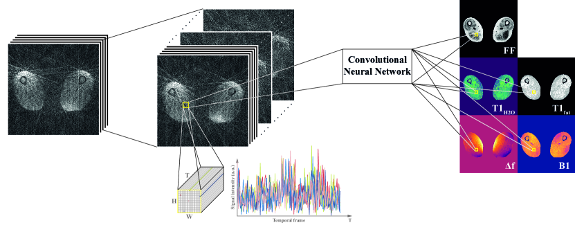
Figure 1: Schematic overview of the proposed MRF reconstruction. Patches of H $\times$ W fingerprints with T temporal frames are extracted from MRF image slices and fed to a CNN, which simultaneously predicts all parametric maps. We used MRF T1-FF (Marty and Carlier, 2019a), an MRF sequence to image diseased skeletal muscle. The parametric maps show the thighs of a 69 years old male patient with inclusion body myositis. FF: fat fraction, T1_H2O: T1 relaxation time of water, T1_fat: T1 relaxation time of fat, $\Delta$f: static magnetic field inhomogeneity, B1: flip angle efficacy.

The hypothesis leading to the design of the proposed CNN architecture is that the reconstruction performance depends on 1) the CNN’s receptive field and 2) the CNN’s capacity. On one hand, the receptive field determines the number of neighboring fingerprints the CNN will use to predict the value of the parametric maps of the central fingerprint. We argue that it is, especially in the case of highly undersampled MRF, beneficial to leverage the spatial correlation among fingerprints but this spatial correlation is limited to a certain extent due to different tissue properties yielding different fingerprints, especially in lesions. Technically speaking, the extent of spatial correlation limits the number of spatial convolutions, i.e., convolutions with kernel sizes larger or equal than $3\times 3$. On the other hand, the reconstruction performance will also be determined by the capacity of the CNN, i.e., the number of learnable parameters or number of convolutional filter weights. A certain capacity is required to extract features that cover the space of possible input fingerprints. Similar as for the receptive field, an appropriate capacity is especially needed when dealing with multiple parametric maps and diverse tissue properties. Having both factors adaptable by an algorithm allows specific tailoring of the CNN-based reconstruction to the MRF sequence at hand.

The schematic overview of the proposed MRF reconstruction is shown in Fig. 1. Let us consider a 2-D+time MRF image slice $I\in\mathbb{C}^{H\times W\times T}$ after NUFFT in the image space with matrix size $H\times W$ and $T$ temporal frames. We aim to find the mapping $\mathcal{M}:I\rightarrow Q$ from the MRF image space to $M$ parametric maps $Q\in\mathbb{R}^{H\times W\times M}$. To learn this mapping, we use a 2-D CNN parametrized by its convolutional filter weights $\theta$. The CNN processes the MRF data patch-wise and treats the temporal frames as channels. Therefore, the CNN is trained to learn the mapping $f:I_{P}\rightarrow Q_{P}$, and estimates the parametric maps by

$$\hat{Q}_{P}=f(I_{P};\theta),$$ (1)

where $f$ the non-linear mapping of the CNN parametrized by $\theta$, and $I_{P}\in\mathbb{C}^{IP_{H}\times IP_{W}\times T}\subset I$ and $Q_{P}\in\mathbb{R}^{QP_{H}\times QP_{W}\times M}\subset Q$ are patches extracted from the 2-D+time MRF image slice and the parametric maps. The CNN reconstructs non-overlapping patches of the parametric maps with size of $QP_{H}\times QP_{W}$. Due to the use of valid convolutions, the input patch size is larger and determined with the CNN’s receptive field $R$ by $IP_{H}\times IP_{W}=QP_{H}+R-1\times QP_{W}+R-1$. Meaning, the input patches are larger than the reconstructed patches at the output of the CNN. We chose the output patch size to be of dimension $QP_{H}\times QP_{W}=32\times 32$ and the input patch dimension was $IP_{H}\times IP_{W}=46\times 46$. Therefore, we used a receptive field of $15\times 15$, i.e., $R=15$. Further for MRF T1-FF, $H=W=350$, $T=175$, and $M=5$ (FF, T1_H2O, T1_fat, $\Delta$f, B1).

2.3 CNN Architecture

The CNN architecture consists of temporal and spatial blocks, which are interleaved within the architecture as shown in Fig. 2a. The temporal blocks extract temporal features from fingerprints while maintaining the receptive field of the CNN. The spatial blocks extract spatially correlated features and increase the receptive field of the CNN. By appropriately setting the number of channels in the temporal and spatial blocks, the capacity can be adjusted. The interleaved blocks are followed by a 1 $\times$ 1 convolution with linear activation function and $M$ channels for predicting $Q_{P}$. Input to the CNN are real-valued $I_{P}$ with real and imaginary parts concatenated as $2T$ channels. A temporal block (Fig. 2b) consists of $1\times 1$ convolutions to not increase the receptive field and follows the design of dense blocks (Huang et al., 2017). They are composed of $L$ layers, and each of them is a sequence of 1 $\times$ 1 convolution, rectified linear unit (ReLU) activation function (Glorot et al., 2011), and batch normalization (BN) (Ioffe and Szegedy, 2015). All convolutions have the same number of $C_{T}$ filters (growth rate), and the feature maps of the preceding layers are concatenated before the next layer to reuse features and facilitate the gradient flow (Huang et al., 2017). A spatial block (Fig. 2c) extracts features from neighboring fingerprints, and, therefore, increases the CNN’s receptive field. It consists of a valid 3 $\times$ 3 convolution with $C_{S}$ filters followed by ReLU activation function, and BN. All convolutions in the CNN are performed with a stride of 1. In principle, the temporal blocks extract a high number of channels, from which the spatial blocks then extract spatially correlated features with an even higher number of parameters (factor 9 due to 3 $\times$ 3 convolution). This increases both the receptive field and the capacity of the CNN.

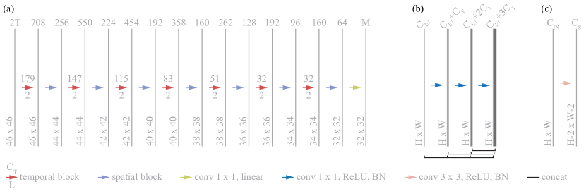
Figure 2: The proposed CNN for MRF reconstruction with a receptive field of $15\times 15$ ($R=15$). (a) the architecture for MRF T1-FF and its (b) temporal (here $L=3$) and (c) spatial blocks. The bars indicate feature maps with the number of channels indicated on the top and the spatial size indicated on the lower left. T: number of temporal frames, M: number of parametric maps, BN: batch normalization, ReLU: rectified linear unit, L: number of layers in a temporal block, $C_{T}$/$C_{S}$: number of channels in a temporal/spatial block, $C_{IN}$: number of input channels, H $\times$ W: feature map size.

2.4 Algorithm

We propose Algorithm 1 to parametrize the temporal and spatial blocks such that the receptive field and the capacity of the CNN are as desired for the MRF sequence to reconstruct. Inputs to the algorithm are the receptive field $R$, the number of parameters $N_{P}$, i.e., the number of learnable weights of all convolutional kernels in the CNN, and the number of non-linearities $N_{L}$, i.e., the number of ReLU activation functions. The number $N_{B}=(R-1)/2$ of temporal and spatial blocks are determined by the receptive field. The number of channels of the spatial blocks $C_{S}$ are chosen such that it gradually decreases down to $C_{S_{stop}}$, in steps of $C_{S_{dec}}$, before the last convolutional filter with linear activation, i.e.,

$$C_{S}=\left(iC_{S_{dec}}+C_{S_{stop}}\right)_{i=N_{B}-1}^{0},$$ (2)

where $(\cdot)$ denotes a sequence (e.g., $C_{S}=(160,128,96,64)$ for $N_{B}=4$, $C_{S_{stop}}=64$, and $C_{S_{dec}}=32$). The number of layers $L$ in each of the temporal blocks are determined by

$$L=\left(\left\lfloor\dfrac{N_{L_{T}}}{N_{B}}\right\rfloor+\mathbbm{1}_{(N_{L_{T}}\mod N_{B})\leq i}\right)_{i=1}^{N_{B}},$$ (3)

where $N_{L_{T}}=N_{L}-N_{B}$ is the remaining number of non-linearities, which corresponds to the total number of convolutional layers in all temporal blocks. The indicator function $\mathbbm{1}$ returns $1$ if the statements is true and $0$ otherwise, and it allows uneven distribution of the convolutional layers among the temporal blocks (e.g., $L=(3,3,2,2)$ for $N_{B}=4$ and $N_{L_{T}}=10$). Given that the number of filters of the temporal blocks $C_{T}$ gradually decrease down to $C_{T_{stop}}$, in steps of $C_{T_{dec}}$, an ideal number of channels in the first temporal block $C_{T_{start}}$ can be calculated such that the total number of learnable convolutional parameters are as close as possible to the desired number of learnable parameters $N_{P}$. Therefore, the desired capacity of the CNN can be matched as close as possible. $C_{T}$ is calculated by

$$C_{T}=\left(g(i)\right)_{i=0}^{N_{B}-1},$$ (4)

with

$$g(x)=\begin{cases}C_{T_{start}}-xC_{T_{dec}},&\text{if }C_{T_{start}}-xC_{T_{dec}}\geq C_{T_{stop}}\\ C_{T_{stop}},&\text{otherwise}\end{cases},$$ (5)

(e.g., $C_{T}=(80,48,32,32)$ for $N_{B}=4$, $C_{T_{start}}=80$, $C_{T_{stop}}=32$, and $C_{T_{dec}}=32$). As we will analyze in Section 3.3, the optimal receptive field of the CNN for the MRF T1-FF sequence is 15 $\times$ 15 with approximately 5 million parameters. Therefore, the architecture consists of seven temporal and spatial blocks. We empirically chose the hyperparameters $N_{L}=21$, $C_{S_{stop}}=64$, $C_{S_{dec}}=32$, $C_{T_{stop}}=32$, and $C_{T_{dec}}=32$, resulting in number of layers $L=(2,2,2,2,2,2,2,2)$, channels of the temporal blocks $C_{T}=(179,147,115,83,51,32,32)$, i.e. $C_{T_{start}}=179$, and channels of the spatial blocks $C_{S}=(256,224,192,160,128,96,64)$.

Algorithm 1 Algorithm for CNN architecture building.

0:  $R$, $N_{P}$, $N_{L}$, $C_{S_{stop}}$, $C_{S_{dec}}$, $C_{T_{stop}}$, $C_{T_{dec}}$

0:  $L,C_{T},C_{S}$

1:  $N_{B}\leftarrow(R-1)/2$, $N_{L_{T}}\leftarrow N_{L}-N_{B}$

2:  Calculate $C_{S}$ with Eq. 2

3:  Calculate $L$ with Eq. 3

4:  $C_{T_{start}}\leftarrow 1$, $N_{P_{best}}\leftarrow\infty$

5:  loop

6:     Calculate $C_{T}$ with Eq. 4

7:     $N_{P}{{}_{current}}\leftarrow calculate\_parameters(L,C_{T},C_{S})$

8:     if $\lvert N_{P}-N_{P}{{}_{current}}\rvert<N_{P_{best}}$ then

9:        $N_{P_{best}}\leftarrow N_{P}{{}_{current}}$

10:        $C_{T_{start}}\leftarrow C_{T_{start}}+1$

11:     else if $\lvert N_{P}-N_{P}{{}_{current}}\rvert>N_{P_{best}}$ then

12:        $C_{T_{start}}\leftarrow C_{T_{start}}-1$

13:        Calculate $C_{T}$ with Eq. 4

14:        return  $L,C_{T},C_{S}$

15:     else

16:        return  $L,C_{T},C_{S}$

17:     end if

18:  end loop

2.5 CNN Training and Implementation

The CNN was trained for 75 epochs with a batch size of 20 randomly selected patches, which we empirically found to be sufficient. The Adam optimizer (Kingma and Ba, 2015) was used to minimize a mean squared error (MSE) loss ($\ell$) with a learning rate of $0.001$, $\beta_{1}=0.9$, and $\beta_{2}=0.999$. Therefore, the learning objective was

$$\min_{\theta}\sum_{i}\ell(f(I_{Pi};\theta),Q_{Pi}).$$ (6)

Before training, we normalized the data subject-wise: The MRF image was normalized to zero mean and unit standard deviation along the real and imaginary parts and each parametric map was rescaled to the range $\left[0,1\right]$ using the minimum and maximum values in the dictionary (see Section 2.1). After inference, the predicted parametric maps were rescaled back to the original dictionary range. The CNN was implemented in TensorFlow 1.10.0 (Google Inc., Mountain View, CA, U.S.) with Python 3.6.7 (Python Software Foundation, Wilmington, DA, U.S.). The training was performed with an NVIDIA TITAN Xp (Nvidia Corporation, Santa Clara, CA, U.S.). For reproducibility, the source code is available online. Further investigation of some architecture hyperparameters can be found in Section 1 of the supplementary material.

2.6 Evaluation and Comparison

Table 1: Clinical and demographic information of the dataset and its distribution into training, validation, and testing splits. Values are given as mean age $\pm$ standard deviation and number of total subjects / number of male subjects / number of thigh images. BMD: Becker muscular distropy, DMD: Duchenne muscular distropy, IBM: Inclusion body myositis.

		Split
Disease	Overall	Training	Validation	Testing
BMD	45.4 $\pm$ 15.0	45.7 $\pm$ 16.9	64.0 $\pm$ 0.0	42.3 $\pm$ 11.3
	19 / 19 / 19	11 / 11 / 11	1 / 1 / 1	7 / 7 / 7
DMD	12.4 $\pm$ 2.2	12.5 $\pm$ 2.3	12.8 $\pm$ 2.5	11.9 $\pm$ 2.0
	25 / 25 / 12	14 / 14 / 8	4 / 4 / 1	7 / 7 / 3
IBM	64.5 $\pm$ 9.6	65.3 $\pm$ 10.4	66.3 $\pm$ 10.3	62.6 $\pm$ 8.3
	70 / 30 / 34	37 / 16 / 13	9 / 4 / 7	24 / 10 / 14
Other	46.9 $\pm$ 14.4	49.2 $\pm$ 14.6	45.0 $\pm$ 16.0	41.7 $\pm$ 12.8
	50 / 19 / 26	32 / 8 / 15	6 / 6 / 4	12 / 5 / 7
Overall	49.0 $\pm$ 21.0	49.7 $\pm$ 21.2	49.1 $\pm$ 23.4	47.6 $\pm$ 19.8
	164 / 93 / 91	94 / 49 / 47	20 / 15 / 13	50 / 29 / 31

We evaluated the performance of the proposed method on a clinical dataset consisting of 164 patients with various neuromuscular diseases (NMDs). The dataset is highly heterogeneous due to the variable phenotypic appearance of lesions in NMDs, and further comprises thigh and leg images. To evaluate the robustness of the methods, we purposely did not apply any stratification regarding disease type, patient sex, patient age, or anatomical region when splitting the dataset into training, validation, and testing splits (n=94/20/50). Table 1 summarizes clinical and demographic characteristics of the dataset. Multimedia files characterizing the heterogeneity of the dataset can be found online as supplementary material.

The dictionary matching reconstruction served as reference for the parametric maps. Quantitative analysis between the dictionary matching and the predicted parametric maps was done according to Zbontar et al. (2018). The normalized root mean squared error (NRMSE), the peak signal-to-noise ratio (PSNR), and the structural similarity index measure (SSIM) (Wang et al., 2004) were calculated at the image level. Due to the quantitative nature of parametric maps, we provide further quantitative analysis based on the coefficient of determination (R²), scatter plots, and Bland-Altman analysis. To this end, we manually segmented regions of interest (ROIs) lying within the major muscles of each subject. The ROIs allowed calculating the mean parametric value within each ROI of each image slice. Then a linear regression between the mean ROI values of the dictionary matching and predicted parametric maps quantified the agreement between the methods. For all evaluation, background voxels (air) were excluded based on an automatically segmented mask generated by thresholding an anatomical image obtained from the MRF image space series (pseudo out-of-phase image (Marty and Carlier, 2019a)). Further, voxels and ROIs with a FF higher than 0.7 were excluded from the evaluation of NRMSE, PSNR, and R² of the T1_H2O map reconstruction due to low confidence of T1_H2O at high FF (Marty and Carlier, 2019a). For the SSIM, we used a window size of 7 $\times$ 7, $K_{1}=0.01$, $K_{2}=0.03$, and $L$ was set to the maximum value of the parametric map.

We compared the proposed method to four other deep learning-based MRF reconstruction, which can be grouped into methods working fingerprint-wise and a method considering spatial neighborhoods of fingerprints. The fingerprint-wise methods comprise Cohen et al. (2018), a neural network with two hidden fully-connected layers, Hoppe et al. (2017), a CNN with four 1-D convolutional layers, and Oksuz et al. (2019), a recurrent neural network (RNN) using a gated recurrent unit with 100 neurons. The spatial method proposed by Fang et al. (2019) works patch-wise using an U-Net-like CNN with pooling operations resulting in a receptive field of 54 $\times$ 54. We implemented all competing methods as described in the papers due to lack of publicly available code. The input and output dimensions were adapted for MRF T1-FF using the complex-valued MRF data as input for all methods. For training, we used the Adam optimizer with a MSE loss as for the proposed method. The batch sizes were set to 100 for the fingerprint-wise methods and the feature extraction module of Fang et al. (2019), and to 20 for the spatially-constrained quantification module of Fang et al. (2019). Training was performed for 25 epochs (Cohen et al., 2018; Hoppe et al., 2017; Oksuz et al., 2019) and 75 epochs for Fang et al. (2019). For each method, the learning rates were chosen from the set $\{0.01,0.001,0.0001\}$ based on the performance on the validation set.

3 Experiments and Results

3.1 Parametric Map Reconstructions

Reconstruction results of the dictionary matching, the proposed method, the best fingerprint-wise method (Oksuz et al., 2019), and the spatial method of Fang et al. (2019) are shown in Fig. 3. Visually, the proposed method achieved the best reconstruction results for all parametric maps. Compared to the dictionary matching, all reconstructions appear to be slightly smoothed. Oksuz et al. (2019) resulted in noisier reconstructions and could not capture elevated T1_H2O. Fang et al. (2019) achieved similar results as the proposed method, but the reconstructions contain artifacts, which are not present for the proposed method. The artifacts possibly originate from the patch-wise processing in combination with padding convolutions, i.e. equal spatial dimension of the input and output of their CNN, resulting in boundary effects. Further, the reconstructions of Fang et al. (2019) appear to be slightly more smooth than the reconstructions of the proposed method. A zoomed-in region with fatty infiltrated muscle and elevated T1_H2O can be found in Section 2 of the supplementary material, showing that Oksuz et al. (2019) fails to reconstruct elevated T1_H2O and that the reconstructions of Fang et al. (2019) contain subtle reconstruction artifacts.

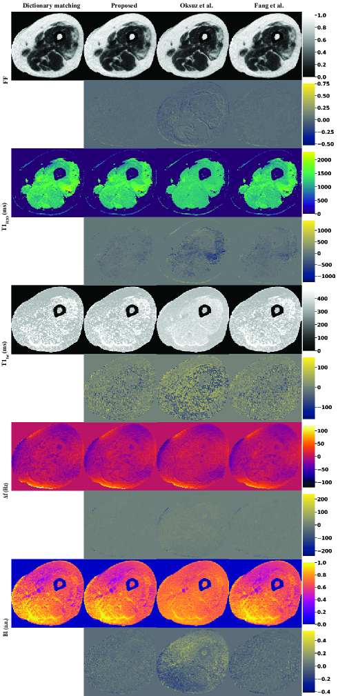
Figure 3: Parametric map reconstruction results of a thigh of a 71 years old male patient with inclusion body myositis. Reconstructions of the dictionary matching, the proposed method, Oksuz et al. (2019), Fang et al. (2019), and the error (dictionary minus reconstruction) are shown. a.u.: arbitrary unit.

Quantitatively, the proposed method achieved the best reconstruction results for the four metrics (Table 2). The parametric maps T1_H2O and T1_fat are the most difficult to reconstruct while for FF, $\Delta$f, and B1 the quantitative results are better. The quality of the agreement is further shown by the quantitative analysis of the ROIs in Fig. 4. The correlations between the CNN and the dictionary matching reconstruction are very high with the Pearson correlation coefficient $r>0.95$ (Fig. 4, left column). Only for T1_H2O and T1_fat, the agreements are slightly decreased with R²s of 0.919 and 0.927. The Bland-Altman plots (Fig. 4, right column) show small to no bias for all five parametric maps, and the 95 % limits of agreement are smaller than the dictionary sampling increment for FF, T1_fat, $\Delta$f, and B1 (cf. Section 2.1). For T1_H2O, the agreement between the methods is approximately $\pm$6 sampling steps or $\pm 60~{}\textnormal{ms}$. Similar plots for the Oksuz et al. (2019) and Fang et al. (2019) can be found in Section 2 of the supplementary material. Reconstructing the parametric maps of one subject (five image slices) required approximately 1 second with the proposed method, which is considerably faster than the dictionary matching requiring up to minutes or even hours depending on the implementation (McGivney et al., 2019). Our dictionary matching implementation requires approximately 5 hours per subject (Marty and Carlier, 2019a). The compared deep learning-based methods are also in the range of 1 second with the fingerprint-wise methods (Hoppe et al., 2017; Cohen et al., 2018) being slightly slower than the proposed CNN, followed by the RNN of Oksuz et al. (2019). The two-stage process of Fang et al. (2019) resulted in the longest reconstruction times.

Table 2: Quantitative results of the proposed and the compared methods. The metrics normalized root mean squared error (NMRSE), peak signal-to-noise ratio (PSNR), structural similarity index measure (SSIM), and coefficient of determination (R²) were calculated for the five parametric maps.

		Method
Metric	Parametric map	Proposed	Hoppe et al.	Cohen et al.	Oksuz et al.	Fang et al.
NRMSE	FF	0.027 $\pm$ 0.004	0.069 $\pm$ 0.007	0.069 $\pm$ 0.006	0.063 $\pm$ 0.007	0.030 $\pm$ 0.004
	T1H2O	0.048 $\pm$ 0.011	0.097 $\pm$ 0.021	0.100 $\pm$ 0.023	0.090 $\pm$ 0.018	0.054 $\pm$ 0.012
	T1fat	0.212 $\pm$ 0.076	0.290 $\pm$ 0.095	0.294 $\pm$ 0.096	0.287 $\pm$ 0.094	0.217 $\pm$ 0.077
	$\Delta$f	0.027 $\pm$ 0.008	0.062 $\pm$ 0.013	0.062 $\pm$ 0.009	0.056 $\pm$ 0.008	0.030 $\pm$ 0.007
	B1	0.056 $\pm$ 0.009	0.107 $\pm$ 0.019	0.117 $\pm$ 0.020	0.107 $\pm$ 0.018	0.062 $\pm$ 0.010
PSNR (dB)	FF	31.6 $\pm$ 1.04	23.3 $\pm$ 0.95	23.4 $\pm$ 0.78	24.1 $\pm$ 0.93	30.7 $\pm$ 1.02
	T1H2O	28.6 $\pm$ 1.75	22.4 $\pm$ 1.71	22.2 $\pm$ 1.76	23.1 $\pm$ 1.54	27.6 $\pm$ 1.69
	T1fat	22.7 $\pm$ 1.85	19.9 $\pm$ 1.35	19.8 $\pm$ 1.30	20.0 $\pm$ 1.38	22.5 $\pm$ 1.78
	$\Delta$f	25.1 $\pm$ 2.11	17.7 $\pm$ 1.96	17.6 $\pm$ 1.62	18.5 $\pm$ 1.63	24.1 $\pm$ 2.02
	B1	27.8 $\pm$ 1.06	22.1 $\pm$ 1.09	21.3 $\pm$ 0.96	22.2 $\pm$ 1.12	26.9 $\pm$ 1.05
SSIM	FF	0.984 $\pm$ 0.011	0.933 $\pm$ 0.039	0.934 $\pm$ 0.038	0.939 $\pm$ 0.036	0.980 $\pm$ 0.014
	T1H2O	0.957 $\pm$ 0.026	0.867 $\pm$ 0.068	0.867 $\pm$ 0.068	0.872 $\pm$ 0.066	0.954 $\pm$ 0.026
	T1fat	0.940 $\pm$ 0.028	0.866 $\pm$ 0.060	0.867 $\pm$ 0.058	0.869 $\pm$ 0.057	0.937 $\pm$ 0.030
	$\Delta$f	0.933 $\pm$ 0.030	0.824 $\pm$ 0.075	0.819 $\pm$ 0.071	0.834 $\pm$ 0.069	0.919 $\pm$ 0.035
	B1	0.965 $\pm$ 0.018	0.894 $\pm$ 0.052	0.893 $\pm$ 0.052	0.895 $\pm$ 0.051	0.959 $\pm$ 0.021
R2	FF	1.000	0.991	0.993	0.994	0.999
	T1H2O	0.919	0.552	0.381	0.648	0.911
	T1fat	0.927	0.693	0.541	0.726	0.908
	$\Delta$f	0.995	0.901	0.901	0.930	0.992
	B1	0.988	0.865	0.785	0.897	0.979

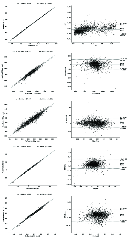
Figure 4: Quantitative agreement between the proposed method and the dictionary matching. (left) Scatter and (right) Bland-Altman plots for the five parametric maps where each dot represents the mean value of the parametric map for a manually segmented ROI lying within a major muscle (n=4392 for FF, T1_fat, $\Delta$f, and B1, and n=3943 for T1_H2O). For the scatter plots, the solid line indicates x=y and the dashed line indicates the fit of the linear regression. For the Bland-Altman plots, the solid line indicates the mean difference and dashed lines indicate the 95 % limits of agreement between the dictionary matching and the proposed method.

3.2 Blurriness of the Parametric Map Reconstructions

In a post hoc analysis, we investigated the blurriness (or smoothness) of the reconstructions of the different methods. We analyzed the energy of the high frequencies in the parametric maps as a metric of blurriness, i.e., the ratio between the energy of the high frequencies and the energy of all frequencies (similar to Section 2.1 of the supplementary material of Fang et al. (2019)). We defined the high frequencies in the spectrum of the parametric maps to be the frequencies above a certain threshold, which we varied from 55 to 95 % because defining one single threshold to separate low and high frequencies was difficult. The energy was defined as the sum of the squared magnitudes. Fig. 5 compares the blurriness of the T1_H2O map reconstruction between the methods (see Section 3 of the supplementary material for the FF, T1_fat, $\Delta$f, and B1 maps). For T1_H2O, all methods clearly produced smoother reconstructions than the dictionary matching. Further, the visually smoother appearance of the reconstructions of Fang et al. (2019) can be confirmed quantitatively. For the FF and $\Delta$f maps, Oksuz et al. (2019) resulted in less smoothing than the dictionary matching, which also confirms the noisy appearance in Fig. 3.

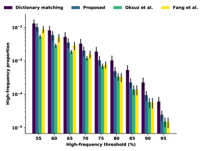
Figure 5: Blurriness of the T1_H2O map reconstruction. The bars indicate mean $\pm$ standard deviation.

3.3 Influence of the Spatial Dimension

The influence of the spatial dimension on the reconstruction quality, or in other words, to what extent the correlation of neighboring fingerprints is beneficial for the reconstruction, is to this date not well studied. Therefore, we varied the receptive field of the proposed CNN from 1 $\times$ 1, which corresponds to fingerprint-wise reconstruction, up to a receptive field of 21 $\times$ 21 using Algorithm 1. We further varied the number of parameters from 1 to 5 million in steps of 1 million (see Section 4 of the supplementary material for configurations). Fig. 6 shows the R² of the T1_H2O map reconstruction depending on the receptive field and the number of parameters. It is visible that fingerprint-wise reconstruction results in significantly inferior reconstructions. Receptive fields around 15 $\times$ 15 seem to perform well with little to no added value when incorporating more fingerprints for the reconstruction. There is no significant change in performance with fewer or more number of parameters. The influence on the parametric maps and metrics except for the T1_H2O map and R² were less accentuated for receptive fields above 5 $\times$ 5. Increasing the receptive field beyond 15 $\times$ 15 had in some cases negative influence (see Section 4 of the supplementary material). Therefore, we did not experiment with receptive fields beyond 21 $\times$ 21. Considering all parametric maps and metrics, we chose a receptive field of 15 $\times$ 15 and 5 million parameters. For comparison, we summarize the receptive field and the number of parameters of the methods of comparison in Table 3.

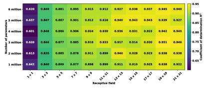
Figure 6: Influence of the spatial receptive field and the number of parameters on the T1_H2O map reconstruction. The numbers denote the R².

Table 3: Architectural summary of the proposed method and the methods of comparison. For Fang et al. (2019) the numbers represent the sum of the numbers of the feature extraction and the spatially-constrained quantification module.

Method	Number of parameters	Number of non-linearities	Receptive field
Proposed	5.00 million	21	15 $\times$ 15
Hoppe et al. (2017)	0.05 million	3	1 $\times$ 1
Cohen et al. (2018)	0.20 million	2	1 $\times$ 1
Oksuz et al. (2019)	0.12 million	1	1 $\times$ 1
Fang et al. (2019)	3.84 million	11	54 $\times$ 54

3.4 Influence of the Temporal Dimension

The influence of the temporal dimension, or in other words, to what extent the temporal frames contribute to the reconstruction, might be of valuable information for the MRF community. To investigate the influence of the temporal dimension, we reformulated the permutation importance by Breiman (2001a, b) for MRF. The permutation importance measures the importance of a variable to a model’s prediction accuracy when the variable is permuted Fisher et al. (2019). Here, the variables are the fingerprint intensities of each temporal frame. We, therefore, randomly permuted the intensities of the $t$-th temporal frame and reconstructed the parametric maps using this permuted MRF data as input. The absolute difference in NRMSE to the non-permuted reconstruction is then considered as the importance of the $t$-th temporal frame of the MRF sequence. The importance of all temporal frames for reconstructing the five parametric maps is shown alongside the MRF sequence in Fig. 7. The first few temporal frames after the non-selective inversion pulse, which should be sensitive to T1, have the highest importance for the reconstruction of the T1_H2O map. For T1_fat the temporal frames after 125 are the most important when water and fat are out of phase. Generally, the temporal frames after the changes in the MRF T1-FF sequence parameters result in high importance for the reconstruction (i.e. at temporal frames 75, 100, 125, and 150).

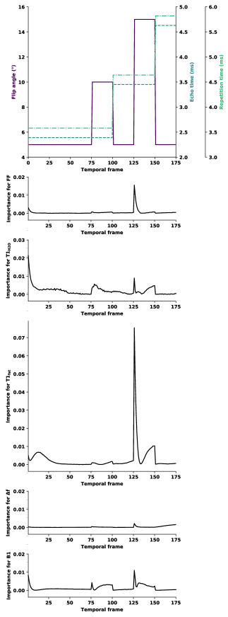
Figure 7: Influence of the temporal frames on the parametric map reconstruction. (first row) The MRF T1-FF sequence parameters and the importance of each temporal frame for (second row) FF, (third row) T1_H2O, (fourth row) T1_fat, (fifth row) $\Delta$f, and (sixth row) B1 reconstruction.

3.5 Robustness to Heterogeneous Morphometric Variations

The results show that the proposed method reconstructs highly heterogeneous morphometric variations in NMD patients well. However, it is unclear how many training subjects are actually needed to obtain a model with good robustness. To investigate this, we randomly selected subsets of a varying number of training subjects from the training set, trained the proposed method with these subsets, and reconstructed the testing set to assess the robustness. The whole process was repeated five times. Fig. 8 summarizes the results of this experiment. With 40 training subjects, the proposed method reconstructs almost identically as when using the entire training set with 94 subjects. However, we also observe that the number of required training subjects depends on the metric of interest.

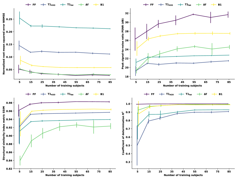
Figure 8: Robustness of the proposed method to heterogeneous morphometric variations depending on the number of training subjects. The CNN was trained with 5, 15, 25, 40, 55, 70, and 85 subjects randomly taken from the training split of 94 subjects. The error bars indicate the standard deviation of five random runs.

3.6 Generalization to Unseen Anatomical Regions

The generalization of deep learning-based MRF reconstruction methods to unseen anatomical regions during training has not been investigated so far, to the best of our knowledge. Therefore, we imaged three NMD patients at three anatomical regions distinctly different to the thigh and leg: the shoulder, the lower abdomen, and the pelvis. MRF acquisition, reconstruction, and evaluation were identical as described in Section 2.1 and Section 2.6. FF and T1_H2O map reconstructions of the proposed method are shown in Fig. 9 and the R²s of the ROI analysis for all parametric maps and methods are summarized in Table 4 (see Section 5 of the supplementary material for all metrics). Qualitatively, the proposed method reconstructed the parametric maps with good quality. In tissues other than skeletal muscle and fatty tissue, the dictionary matching and the proposed reconstruction resulted in noisy parametric maps, which was expected due to the MRF T1-FF sequence’s purpose. Quantitatively, the proposed approach resulted in a slight decrease of performance for FF, $\Delta$f, and B1. For T1_H2O and T1_fat, the decrease is more significant (cf. Table 4). This decrease was even more accentuated for the method of Fang et al. (2019). And, despite working fingerprint-wise, the method of Oksuz et al. (2019) resulted in the worst reconstructions for unseen anatomical regions.

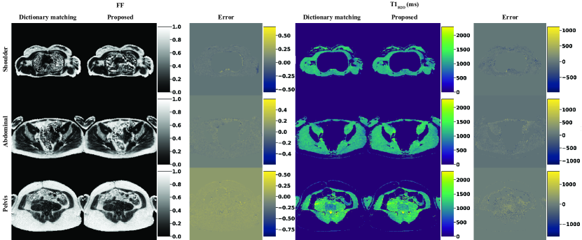
Figure 9: Generalization of the proposed method to unseen anatomical regions. The CNN trained on thigh and leg images has been applied to reconstruct shoulder, lower abdominal (proximal to pelvis), and pelvis MRF T1-FF acquisitions. Regions with noisy dictionary matching reconstructions have been masked in the error map due to the insensitivity of MRF T1-FF to tissues other than skeletal muscle and fatty tissue.

Table 4: Quantitative results for the reconstruction of unseen anatomical regions. The numbers denote the R².

	Parametric map
Method	FF	T1H2O	T1fat	$\Delta$f	B1
Proposed	0.978	0.862	0.804	0.991	0.989
Oksuz et al. (2019)	0.746	0.409	0.420	0.862	0.760
Fang et al. (2019)	0.973	0.758	0.787	0.970	0.980

4 Discussion

We have investigated the reconstruction of parametric maps from MRF using CNNs. Driven by the hypothesis that the reconstruction performance depends on the incorporation of neighboring fingerprints, i.e., the receptive field of the CNN, and the capacity, i.e., the number of parameters of the CNN, we have designed an algorithm for flexible architecture building based on the specific requirements of the MRF sequence to reconstruct. The configuration for MRF T1-FF was empirically determined to be a receptive field of 15 $\times$ 15 with five million parameters. With this configuration, we have shown that the proposed method yields accurate parametric map reconstruction, independent of the morphometric heterogeneity of imaged patients as well as unseen anatomical regions. The method is fast, enabling reconstruction of parametric maps in a clinical setting. Further, as shown qualitatively and quantitatively, better reconstruction results were achieved with the proposed method as compared to other deep learning-based methods.

The proposed method yielded an absolute reconstruction error lower than the dictionary sampling increment for all except the T1_H2O map (Fig. 4). Therefore, we argue that there is no difference in reconstruction accuracy between the proposed method and the dictionary matching for the FF, T1_fat, $\Delta$f, and B1 maps. Based on the observed differences for T1_H2O map reconstructions, we concede that the sensitivity of MRF T1-FF to T1_H2O might not be optimal. The fingerprints encode T1_H2O to some extent, but for nuances in T1_H2O, they contain probably more noise than discriminative patterns. This observation can also be confirmed when comparing simulated fingerprints with close T1_H2O values (see Section 6 of the supplementary material). Further, large receptive fields were mainly beneficial for T1_H2O with a lower effect on the other parametric maps. The CNN might compensate for the low signal-to-noise ratio by regularizing spatially. We, therefore, also believe that modifications of the CNN architecture will bring limited additional reconstruction performance and that efforts are better invested at optimizing the MRF sequence than the deep learning-based reconstruction such as done recently (Cohen and Rosen, 2017; Zhao et al., 2019; Lee et al., 2019).

We have analyzed that the receptive field, i.e., considering a spatial neighborhood of fingerprints, influences the reconstruction performance. On the one hand, fingerprint-wise reconstruction (receptive field of 1 $\times$ 1) is significantly inferior to spatial reconstruction. We attribute this mainly to the potentially high correlation of neighboring fingerprints coupled with the strong undersampling of MRF. On the other hand, spatial reconstruction has improved the reconstruction only to some extent (Fig. 6). Regarding the blurriness of the reconstruction, the optimal receptive field is a difficult choice but it lies likely between fingerprint-wise reconstruction and the large receptive field of Fang et al. (2019) (Fig. 5). Further, we have observed a larger decrease in performance for Fang et al. (2019) when reconstructing unseen anatomical regions. We attribute this decrease to the method’s large receptive field of 54 $\times$ 54 where fingerprints without valuable information, possibly influenced by susceptibility artifacts, were included in the reconstruction (cf. noisy tissues in the parametric maps). Therefore, we conclude that pooling operations with subsequent deconvolution operations, as e.g. in the U-Net-like architecture of Fang et al. (2019), are not needed for MRF reconstruction. Clearly, spatial regularization is superior to fingerprint-wise reconstruction but its extent dependents almost certainly on the MRF sequence due to various factors such as the sensitivity to the MR parameters, k-space sampling, in-plane voxel size, among others. But with the proposed algorithm, investigating this aspect becomes straightforward due to the CNN’s adaptability.

We have studied the influence of the temporal frames on the parametric map reconstruction. Such reconstruction interpretability might be useful for further developments of MRF reconstruction, as well as the MRF sequence development itself. As expected, the inversion pulse yields high importance to the first few temporal frames for T1 parameters. The general correlation between abrupt sequence parameter changes and high importance hints at highly sensitive temporal frames to MR parameters, and, therefore, rich information for the reconstruction. Fang et al. (2019) proposed to reduce the time of the MRF acquisition by considering only the first fractions of the temporal frames. However, such an approach, although being straightforward, might be suboptimal considering that not all temporal frames might be of equal importance for the MRF reconstruction. For instance, in the case of MRF T1-FF, the temporal frames 50 to 75 as well as the last 25 temporal frames might be useless for the reconstruction, containing maybe redundant or irrelevant information. An acceleration of the MRF acquisition might be achieved by discarding these temporal frames without sacrificing reconstruction performance.

We have demonstrated an excellent robustness of the proposed method to heterogeneous morphometric variations and unseen anatomical regions, a desired key property for image reconstruction (Knoll et al., 2019). Previous MRF reconstruction studies were performed on small cohorts of healthy volunteers (Cohen et al., 2018; Balsiger et al., 2018; Fang et al., 2018, 2019; Golbabaee et al., 2019; Song et al., 2019), limiting their clinical significance. Here, we have presented, to the best of our knowledge, the first study on reconstructing highly undersampled MRF of patient data only (Table 1). To study the robustness of a method, NMDs are an excellent subject given their large phenotypic variability, the broad range of affected anatomical regions as well as patient age distribution. Our approach seems to be rather insensitive to such variability, which we also attribute to the large and heterogeneous training data. We have found that it is also possible to achieve good robustness with fewer training data (Fig. 8). However, the robustness is dependent on the parametric map as well as the desired property of the reconstruction (e.g., structural similarity and signal-to-noise). Further, we have found that the number of parameters of the CNN is a rather insensitive characteristic (Fig. 6). Nor a decrease in performance with fewer neither overfitting with more learnable parameters have been observed, indicating that a performance benefit can primarily be attributed to the spatial regularization (i.e., the receptive field). Reproducing the results of Fig. 8 with varying number of parameters might give additional insights into a possible link between robustness and the number of parameters but is computationally unfeasible due to the immense number of training runs needed.

Our study has several limitations, which we plan to address in future work. First and foremost, the absence of a better reference for comparison than the dictionary matching is a significant issue. Ideally, the CNN reconstruction should be compared to parametric maps obtained by gold standard parametric mapping (Balsiger et al., 2018). However, while this is possible for FF (e.g., using 3-point Dixon (Glover and Schneider, 1991)), there exists no MR sequence for T1_H2O mapping in fatty infiltrated tissue. Second, the optimal MRF data handling is still subject to further research. We have investigated several variants (see Section 1.3 of the supplementary material), but there are certainly open questions such as the complex-valued nature of the MRF data, e.g., reconstruction by complex-valued CNN (Virtue et al., 2017; Trabelsi et al., 2018). Also, the modeling of the temporal domain, e.g., by RNNs as presented by Oksuz et al. (2019) or by 3-D CNNs, needs further research. Finally, we can not make any statements of the performance on other MRF sequences. Ideally, a completely independent dataset acquired with another MRF sequence and with other diseases should be available to demonstrate applicability among MRF sequences.

In conclusion, we proposed an adaptable CNN for accurate and fast reconstruction of parametric maps from MRF. We demonstrated that incorporating a spatial neighborhood of fingerprints during the reconstruction is beneficial and that we achieved excellent reconstruction accuracy and robustness to heterogeneous patient data. The proposed method could enable MRF beyond clinical research studies.

References

- Assländer et al. (2018) Assländer, J., Cloos, M.A., Knoll, F., Sodickson, D.K., Hennig, J., Lattanzi, R., 2018. Low Rank Alternating Direction Method of Multipliers Reconstruction for MR Fingerprinting. Magnetic Resonance in Medicine 79, 83–96. doi:10.1002/mrm.26639.
- Balsiger et al. (2019) Balsiger, F., Scheidegger, O., Carlier, P.G., Marty, B., Reyes, M., 2019. On the Spatial and Temporal Influence for the Reconstruction of Magnetic Resonance Fingerprinting, in: Cardoso, M.J., Feragen, A., Glocker, B., Konukoglu, E., Oguz, I., Unal, G., Vercauteren, T. (Eds.), Proceedings of The 2nd International Conference on Medical Imaging with Deep Learning, PMLR, London. pp. 27–38.
- Balsiger et al. (2018) Balsiger, F., Shridhar Konar, A., Chikop, S., Chandran, V., Scheidegger, O., Geethanath, S., Reyes, M., 2018. Magnetic Resonance Fingerprinting Reconstruction via Spatiotemporal Convolutional Neural Networks, in: Knoll, F., Maier, A., Rueckert, D. (Eds.), Machine Learning for Medical Image Reconstruction. Springer, Cham. volume 11074 of Lecture Notes in Computer Science, pp. 39–46. doi:10.1007/978-3-030-00129-2_5.
- Breiman (2001a) Breiman, L., 2001a. Random Forests. Machine Learning 45, 5–32. doi:10.1023/A:1010933404324.
- Breiman (2001b) Breiman, L., 2001b. Statistical Modeling: The Two Cultures. Statistical Science 16, 199–231. doi:10.1214/SS/1009213726.
- Carlier et al. (2016) Carlier, P.G., Marty, B., Scheidegger, O., Loureiro de Sousa, P., Baudin, P.Y., Snezhko, E., Vlodavets, D., 2016. Skeletal Muscle Quantitative Nuclear Magnetic Resonance Imaging and Spectroscopy as an Outcome Measure for Clinical Trials. Journal of Neuromuscular Diseases 3, 1–28. doi:10.3233/JND-160145.
- Cauley et al. (2015) Cauley, S.F., Setsompop, K., Ma, D., Jiang, Y., Ye, H., Adalsteinsson, E., Griswold, M.A., Wald, L.L., 2015. Fast Group Matching for MR Fingerprinting Reconstruction. Magnetic Resonance in Medicine 74, 523–528. doi:10.1002/mrm.25439.
- Cohen and Rosen (2017) Cohen, O., Rosen, M.S., 2017. Algorithm comparison for schedule optimization in MR fingerprinting. Magnetic Resonance Imaging 41, 15–21. doi:10.1016/J.MRI.2017.02.010.
- Cohen et al. (2018) Cohen, O., Zhu, B., Rosen, M.S., 2018. MR fingerprinting Deep RecOnstruction NEtwork (DRONE). Magnetic Resonance in Medicine 80, 885–894. doi:10.1002/mrm.27198.
- Davies et al. (2014) Davies, M., Puy, G., Vandergheynst, P., Wiaux, Y., 2014. A Compressed Sensing Framework for Magnetic Resonance Fingerprinting. SIAM Journal on Imaging Sciences 7, 2623–2656. doi:10.1137/130947246.
- Fang et al. (2019) Fang, Z., Chen, Y., Liu, M., Xiang, L., Zhang, Q., Wang, Q., Lin, W., Shen, D., 2019. Deep Learning for Fast and Spatially-Constrained Tissue Quantification from Highly-Accelerated Data in Magnetic Resonance Fingerprinting. IEEE Transactions on Medical Imaging 38, 2364–2374. doi:10.1109/TMI.2019.2899328.
- Fang et al. (2018) Fang, Z., Chen, Y., Liu, M., Zhan, Y., Lin, W., Shen, D., 2018. Deep Learning for Fast and Spatially-Constrained Tissue Quantification from Highly-Undersampled Data in Magnetic Resonance Fingerprinting (MRF), in: Shi, Y., Suk, H.I., Liu, M. (Eds.), Machine Learning in Medical Imaging. Springer, Cham. volume 11046 of Lecture Notes in Computer Science, pp. 398–405. doi:10.1007/978-3-030-00919-9_46.
- Fessler and Sutton (2003) Fessler, J., Sutton, B., 2003. Nonuniform Fast Fourier Transforms Using Min-Max Interpolation. IEEE Transactions on Signal Processing 51, 560–574. doi:10.1109/TSP.2002.807005.
- Fisher et al. (2019) Fisher, A., Rudin, C., Dominici, F., 2019. All Models are Wrong, but Many are Useful: Learning a Variable’s Importance by Studying an Entire Class of Prediction Models Simultaneously. Journal of Machine Learning Research 20, 1–81.
- Glorot et al. (2011) Glorot, X., Bordes, A., Bengio, Y., 2011. Deep Sparse Rectifier Neural Networks, in: Gordon, G., Dunson, D., Dudík, M. (Eds.), International Conference on Artificial Intelligence and Statistics, PMLR, Fort Lauderdale. pp. 315–323.
- Glover and Schneider (1991) Glover, G.H., Schneider, E., 1991. Three-point Dixon technique for true water/fat decomposition with B0 inhomogeneity correction. Magnetic Resonance in Medicine 18, 371–383. doi:10.1002/mrm.1910180211.
- Golbabaee et al. (2019) Golbabaee, M., Chen, D., Gómez, P.A., Menzel, M.I., Davies, M.E., 2019. Geometry of Deep Learning for Magnetic Resonance Fingerprinting, in: IEEE International Conference on Acoustics, Speech and Signal Processing (ICASSP), IEEE. pp. 7825–7829. doi:10.1109/ICASSP.2019.8683549.
- Gómez et al. (2016) Gómez, P.A., Molina-Romero, M., Ulas, C., Bounincontri, G., Sperl, J.I., Jones, D.K., Menzel, M.I., Menze, B.H., 2016. Simultaneous Parameter Mapping, Modality Synthesis, and Anatomical Labeling of the Brain with MR Fingerprinting, in: Ourselin, S., Joskowicz, L., Sabuncu, M.R., Unal, G., Wells, W. (Eds.), Medical Image Computing and Computer-Assisted Intervention – MICCAI 2016, Springer International Publishing, Cham. pp. 579–586. doi:10.1007/978-3-319-46726-9_67.
- Hoppe et al. (2017) Hoppe, E., Körzdörfer, G., Würfl, T., Wetzl, J., Lugauer, F., Pfeuffer, J., Maier, A., 2017. Deep Learning for Magnetic Resonance Fingerprinting: A New Approach for Predicting Quantitative Parameter Values from Time Series., in: Röhrig, R., Timmer, A., Binder, H., Sax, U. (Eds.), German Medical Data Sciences: Visions and Bridges, Oldenburg, Oldenburg. pp. 202–206. doi:10.3233/978-1-61499-808-2-202.
- Huang et al. (2017) Huang, G., Liu, Z., van der Maaten, L., Weinberger, K.Q., 2017. Densely Connected Convolutional Networks, in: IEEE Conference on Computer Vision and Pattern Recognition (CVPR), IEEE. pp. 2261–2269. doi:10.1109/CVPR.2017.243.
- Ioffe and Szegedy (2015) Ioffe, S., Szegedy, C., 2015. Batch Normalization: Accelerating Deep Network Training by Reducing Internal Covariate Shift, in: Bach, F., Blei, D. (Eds.), International Conference on Machine Learning, PMLR, Lille. pp. 448–456.
- Kingma and Ba (2015) Kingma, D.P., Ba, J.L., 2015. Adam: A Method for Stochastic Optimization, in: International Conference on Learning Representations. arXiv:1412.6980.
- Knoll et al. (2019) Knoll, F., Hammernik, K., Kobler, E., Pock, T., Recht, M.P., Sodickson, D.K., 2019. Assessment of the generalization of learned image reconstruction and the potential for transfer learning. Magnetic Resonance in Medicine 81, 116--128. doi:10.1002/mrm.27355.
- Lee et al. (2019) Lee, P.K., Watkins, L.E., Anderson, T.I., Buonincontri, G., Hargreaves, B.A., 2019. Flexible and efficient optimization of quantitative sequences using automatic differentiation of Bloch simulations. Magnetic Resonance in Medicine 82, 1438--1451. doi:10.1002/mrm.27832.
- Lima da Cruz et al. (2019) Lima da Cruz, G., Bustin, A., Jaubert, O., Schneider, T., Botnar, R.M., Prieto, C., 2019. Sparsity and locally low rank regularization for MR fingerprinting. Magnetic Resonance in Medicine 81, 3530--3543. doi:10.1002/mrm.27665.
- Ma et al. (2013) Ma, D., Gulani, V., Seiberlich, N., Liu, K., Sunshine, J.L., Duerk, J.L., Griswold, M.A., 2013. Magnetic resonance fingerprinting. Nature 495, 187--192. doi:10.1038/nature11971.
- Marty and Carlier (2019a) Marty, B., Carlier, P.G., 2019a. MR fingerprinting for water T1 and fat fraction quantification in fat infiltrated skeletal muscles. Magnetic Resonance in Medicine 83, 621--634. doi:10.1002/mrm.27960.
- Marty and Carlier (2019b) Marty, B., Carlier, P.G., 2019b. Physiological and pathological skeletal muscle T1 changes quantified using a fast inversion-recovery radial NMR imaging sequence. Scientific Reports 9, 6852. doi:10.1038/s41598-019-43398-x.
- Mazor et al. (2018) Mazor, G., Weizman, L., Tal, A., Eldar, Y.C., 2018. Low-rank magnetic resonance fingerprinting. Medical Physics 45, 4066--4084. doi:10.1002/mp.13078.
- McGivney et al. (2019) McGivney, D.F., Boyacıoğlu, R., Jiang, Y., Poorman, M.E., Seiberlich, N., Gulani, V., Keenan, K.E., Griswold, M.A., Ma, D., 2019. Magnetic resonance fingerprinting review part 2: Technique and directions. Journal of Magnetic Resonance Imaging 51, 993--1007. doi:10.1002/jmri.26877.
- McGivney et al. (2014) McGivney, D.F., Pierre, E., Ma, D., Jiang, Y., Saybasili, H., Gulani, V., Griswold, M.A., 2014. SVD Compression for Magnetic Resonance Fingerprinting in the Time Domain. IEEE Transactions on Medical Imaging 33, 2311--2322. doi:10.1109/TMI.2014.2337321.
- Oksuz et al. (2019) Oksuz, I., Cruz, G., Clough, J., Bustin, A., Fuin, N., Botnar, R.M., Prieto, C., King, A.P., Schnabel, J.A., 2019. Magnetic Resonance Fingerprinting using Recurrent Neural Networks, in: International Symposium on Biomedical Imaging, IEEE. pp. 1537--1540. doi:10.1109/ISBI.2019.8759502.
- Paoletti et al. (2019) Paoletti, M., Pichiecchio, A., Cotti Piccinelli, S., Tasca, G., Berardinelli, A.L., Padovani, A., Filosto, M., 2019. Advances in Quantitative Imaging of Genetic and Acquired Myopathies: Clinical Applications and Perspectives. Frontiers in Neurology 10, 78. doi:10.3389/fneur.2019.00078.
- Pierre et al. (2016) Pierre, E.Y., Ma, D., Chen, Y., Badve, C., Griswold, M.A., 2016. Multiscale Reconstruction for MR Fingerprinting. Magnetic Resonance in Medicine 75, 2481--2492. doi:10.1002/mrm.25776.
- Poorman et al. (2019) Poorman, M.E., Martin, M.N., Ma, D., McGivney, D.F., Gulani, V., Griswold, M.A., Keenan, K.E., 2019. Magnetic resonance fingerprinting Part 1: Potential uses, current challenges, and recommendations. Journal of Magnetic Resonance Imaging 51, 675--692. doi:10.1002/jmri.26836.
- Song et al. (2019) Song, P., Eldar, Y.C., Mazor, G., Rodrigues, M.R., 2019. HYDRA: Hybrid Deep Magnetic Resonance Fingerprinting. Medical Physics 46, 4951--4969. doi:10.1002/mp.13727, arXiv:1902.02882.
- Trabelsi et al. (2018) Trabelsi, C., Bilaniuk, O., Zhang, Y., Serdyuk, D., Subramanian, S., Santos, J.F., Mehri, S., Rostamzadeh, N., Bengio, Y., Pal, C.J., 2018. Deep Complex Networks, in: International Conference on Learning Representations. arXiv:1705.09792.
- Virtue et al. (2017) Virtue, P., Yu, S.X., Lustig, M., 2017. Better than Real: Complex-valued Neural Nets for MRI Fingerprinting, in: IEEE International Conference on Image Processing (ICIP), IEEE. pp. 3953--3957. doi:10.1109/ICIP.2017.8297024.
- Wang et al. (2004) Wang, Z., Bovik, A., Sheikh, H., Simoncelli, E., 2004. Image Quality Assessment: From Error Visibility to Structural Similarity. IEEE Transactions on Image Processing 13, 600--612. doi:10.1109/TIP.2003.819861.
- Zbontar et al. (2018) Zbontar, J., Knoll, F., Sriram, A., Muckley, M.J., Bruno, M., Defazio, A., Parente, M., Geras, K.J., Katsnelson, J., Chandarana, H., Zhang, Z., Drozdzal, M., Romero, A., Rabbat, M., Vincent, P., Pinkerton, J., Wang, D., Yakubova, N., Owens, E., Zitnick, C.L., Recht, M.P., Sodickson, D.K., Lui, Y.W., 2018. fastMRI: An Open Dataset and Benchmarks for Accelerated MRI. arXiv preprint arXiv:1811.08839 arXiv:1811.08839.
- Zhao et al. (2019) Zhao, B., Haldar, J.P., Liao, C., Ma, D., Jiang, Y., Griswold, M.A., Setsompop, K., Wald, L.L., 2019. Optimal Experiment Design for Magnetic Resonance Fingerprinting: Cramér-Rao Bound Meets Spin Dynamics. IEEE Transactions on Medical Imaging 38, 844--861. doi:10.1109/TMI.2018.2873704.
- Zhao et al. (2018) Zhao, B., Setsompop, K., Adalsteinsson, E., Gagoski, B., Ye, H., Ma, D., Jiang, Y., Ellen Grant, P., Griswold, M.A., Wald, L.L., 2018. Improved Magnetic Resonance Fingerprinting Reconstruction With Low-Rank and Subspace Modeling. Magnetic Resonance in Medicine 79, 933--942. doi:10.1002/mrm.26701.