A notion of equivalence for linear complementarity problems with application to the design of non-smooth bifurcations

Abstract

Many systems of interest to control engineering can be modeled by linear complementarity problems. We introduce a new notion of equivalence between linear complementarity problems that sets the basis to translate the powerful tools of smooth bifurcation theory to this class of models. Leveraging this notion of equivalence, we introduce new tools to analyze, classify, and design non-smooth bifurcations in linear complementarity problems and their interconnection.

1 Introduction

Bifurcation theory is one of the most successful tools for the analysis of nonlinear dynamical systems that depend on a control parameter. The theory is firmly grounded on the classical implicit function theorem (Dontchev and Rockafellar, 2014; Golubitsky and Schaeffer, 1985), and therefore, it requires smoothness of the maps under study. However, from a practical viewpoint, it is common to approximate complicated nonlinear maps by simpler models. In such situations, the resulting approximation may be non-smooth.

Linear complementarity problems are non-smooth problems that arise in fields of science such as economics (Nagurney, 1999), electronics (Acary et al., 2011), mechanics (Brogliato, 1999), mathematical programming (Murty, 1988), general systems theory (van der Schaft and Schumacher, 1998), etc. They serve as a departing point in the analysis of problems with unilateral constraints, and also arise as piecewise linear approximations of nonlinear models (Leenaerts and Bokhoven, 1998).

Recently, there have been some attempts to extend bifurcation theory towards the non-smooth setting, see e.g. Di Bernardo et al. (2008); Leine and Nijmeijer (2004); Simpson (2010). However, the emphasis has been directed towards analysis of discontinuous systems, and very little is known on bifurcations in complementarity systems.

The purpose of this paper is to provide a methodology for the realization of equilibrium bifurcations in linear complementarity problems. The proposed framework mimics, up to certain extent, the smooth program proposed by Arnold et al. (1985) and relies on tools from non-smooth analysis and linear algebra. To achieve this, the concept of topological equivalence in complementarity systems is introduced. We focus on static models that arise as the steady-state equations of piecewise linear dynamical systems. Thanks to the piecewise linear structure of the problem, the introduced equivalence is always global, which constitutes a major difference with respect to smooth bifurcation theories. This fundamental concept allows us to provide a complete classification of planar complementarity problems.

The paper is organized as follows. Section 2 describes the linear complementarity problem and related concepts. Section 3 constitutes the main body of the paper and addresses the problem of topological equivalence between LCP’s. Afterwards, an interconnection approach for the realization of bifurcations is presented, together with an example applied to the non-smooth pleat and the pitchfork singularity. Finally, the paper ends with some conclusions and future research directions in Section 4.

2 Preliminaries

2.1 Linear Complementarity Problems

The linear complementarity problem (LCP) is defined as follows.

Definition 1.

Given a vector $q\in\mathbb{R}^{n}$ and a matrix $M\in\mathbb{R}^{n\times n}$, the LCP $(M,q)$ consists in finding vectors $z,w\in\mathbb{R}^{n}$ such that

$$\begin{cases}w=Mz+q\\ \mathbb{R}_{+}^{n}\ni w\perp z\in\mathbb{R}_{+}^{n}\end{cases}$$ (1)

where the second relation, called the complementary condition, is the short form of the following three conditions: $w\in\mathbb{R}_{+}^{n}$, $z\in\mathbb{R}_{+}^{n}$, and $w^{\top}z=0$.

In what follows, we introduce some concepts that will be useful for studying the geometric structure of LCPs. Given $M$ and an index set $\alpha\subseteq\left\{1,\dots,n\right\}$, we define the complementary matrix $C_{M}(\alpha)$ as

$$C_{M}(\alpha)_{\boldsymbol{\cdot}j}=\begin{cases}-M_{\boldsymbol{\cdot}j}&\quad\text{if $j\in\alpha$}\\ I_{\boldsymbol{\cdot}j}&\quad\text{if $j\not\in\alpha$}\end{cases}\;,$$

where the subscript $\boldsymbol{\cdot}j$ denotes the $j$-th column. Now define the piecewise-linear function

$$f_{M}(x)=C_{-M}(\alpha)x\;,\quad x\in\operatorname{pos}C_{I}(\alpha)\;,$$ (2)

where $\operatorname{pos}C_{I}(\alpha)$ is the cone generated by the columns of $C_{I}(\alpha)$. Note that the cones $\operatorname{pos}C_{I}(\alpha)$ are simply the $2^{n}$ orthants in $\mathbb{R}^{n}$ indexed by $\alpha\subseteq\{1,\dots,n\}$, and that

$$f_{M}(\operatorname{pos}C_{I}(\alpha))=\operatorname{pos}C_{M}(\alpha)\;.$$

Proposition 2 (Cottle et al. (2009)).

Let $z\in\mathbb{R}^{n}$ be a solution of the LCP $(M,q)$, then $x=w-z\in\mathbb{R}^{n}$ is a solution of

$$f_{M}(x)=q\;.$$ (3)

Conversely, let $x\in\mathbb{R}^{n}$ be a solution of (3), then $z=\operatorname{Proj}_{\mathbb{R}_{+}^{n}}(-x)\in\mathbb{R}_{+}^{n}$ is a solution of the LCP $(M,q)$.

Henceforth, we treat the LCP $(M,q)$ and (3) as identical problems, in the sense that we only need to know the solution of one of them in order to know the solution of the other.

The solutions of the LCP $(M,q)$ depend on the geometry of the complementary cones $\operatorname{pos}C_{M}(\alpha)$. More precisely, there exists at least one solution $x$ of (3) for every $\alpha$ such that $q\in\operatorname{pos}C_{M}(\alpha)$. If $C_{M}(\alpha)$ is nonsingular the solution is unique, whereas there exists a continuum of solutions if $C_{M}(\alpha)$ is singular. Thus, for a given $q$, there can be no solutions, there can be one solution, multiple isolated solutions, or a continuum of solutions, depending on how many complementary cones $q$ belongs to and their properties.

2.2 Bifurcations in LCPs

In practical applications, the vector $q$ depends on a control, or bifurcation parameter $\lambda\in\mathbb{R}$. The bifurcation parameter can be an applied voltage or current in electronic circuits, a force or a torque in a mechanical system, or the amount of capital injection in an economic system. The goal of bifurcation theory is to understand how the number of solutions changes as the bifurcation parameter is varied. In LCPs we let $q=\bar{q}(\lambda),$ where $\bar{q}:\mathbb{R}\to\mathbb{R}^{n}$ is at least continuous, although more regularity constraints can be imposed as needed. The mapping $\bar{q}$ defines a continuous curve, or path in $\mathbb{R}^{n}$. As $\lambda$ lets $q$ move along this path, the number of solution to the LCPs might change. Points where the number of solutions change are called bifurcation points.

Example 3.

Let us illustrate this idea in the simple case where the path is a line segment joining two distinct points $q_{i}\in\mathbb{R}^{2}$, $i\in\{0,1\}$, that is,

$$\bar{q}(\lambda)=(1-\lambda)q_{0}+\lambda q_{1},\quad\lambda\in[0,1].$$

In addition, let us set the matrix $M$ as

$$M=\begin{bmatrix}1&2\\ 2&1\end{bmatrix}$$ (4)

and proceed to analyze the two cases shown in Fig. 1.

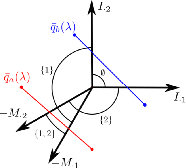
Figure 1: Cone configuration for matrix $M$ in (4). The thick black lines depict the generators of the complementary cones $\operatorname{pos}C_{M}(\alpha)$, $\alpha\subseteq\{1,2\}$, whereas the arcs denote the complementary cones.

Case a) We take the path $\bar{q}_{a}(\lambda)$ given by

$$\bar{q}_{a}(\lambda)=(1-\lambda)\begin{bmatrix}-4\\ 0\end{bmatrix}+\lambda\begin{bmatrix}0\\ -4\end{bmatrix}\;,\quad\lambda\in[0,1]\;.$$ (5)

According to Proposition 2, solving the LCP $(M,\bar{q}_{a}(\lambda))$ is equivalent to finding $x\in\mathbb{R}^{2}$ satisfying

$$C_{-M}(\alpha)x=\bar{q}_{a}(\lambda),\quad\text{ s.t. }x\in\operatorname{pos}C_{I}(\alpha)\;,$$ (6)

for $\alpha\subseteq\{1,2\}$. Noting that $C_{M}(\alpha)=C_{-M}(\alpha)C_{I}(\alpha)$ for any $\alpha\subseteq\{1,2\}$, it follows that the solutions to (6) are given by

$${\bigcup}_{\alpha\subseteq\{1,2\}}S_{\alpha}$$ (7)

where

$$S_{\alpha}=\big{\{}(x,\lambda)\in\mathbb{R}^{2}\times[0,1]\mid\exists\;p_{\lambda}(\alpha)\in\mathbb{R}_{+}^{2}\;:\\ x=C_{I}(\alpha)p_{\lambda}(\alpha)\text{ and }\bar{q}_{a}(\lambda)=C_{M}(\alpha)p_{\lambda}(\alpha)\big{\}}$$ (8)

Roughly speaking, in order to solve the parametrized LCP $(M,\bar{q}(\lambda))$ we need to find $p_{\lambda}(\alpha)$ (the representation of $\bar{q}(\lambda)$ in terms of the generators of the $\alpha$-th complementary cone). Computing these explicitly and taking $\alpha=\emptyset\subset\{1,2\}$ we get

$$p_{\lambda}(\emptyset)=C_{M}(\emptyset)\bar{q}_{a}(\lambda)=\begin{bmatrix}4\lambda-4\\ -4\lambda\end{bmatrix}\;,$$

and it follows that $p_{\lambda}(\emptyset)\notin\mathbb{R}_{+}^{2}$ for any $\lambda\in\mathbb{R}$. Therefore, $S_{\emptyset}=\emptyset$. Now, for $\alpha=\{1\}\subset\{1,2\}$ we get that

$$p_{\lambda}(\{1\})=C_{M}(\{1\})\bar{q}_{a}(\lambda)=\begin{bmatrix}4-4\lambda\\ 8-12\lambda\end{bmatrix}.$$

It follows that $p_{\lambda}(\{1\})\in\mathbb{R}_{+}^{2}$ for $\lambda\in(-\infty,2/3]$. Hence,

$$S_{\{1\}}=\left\{(x,\lambda)\in\mathbb{R}^{2}\times[0,2/3]\mid x=\begin{bmatrix}4\lambda-4\\ 8-12\lambda\end{bmatrix}\right\}$$

Similarly, for $\alpha=\{2\}$ and $\alpha=\{1,2\}$ we have, respectively,

$$S_{\{2\}} =\left\{(x,\lambda)\in\mathbb{R}^{2}\times[1/3,1]\mid x=\begin{bmatrix}-4+12\lambda\\ -4\lambda\end{bmatrix}\right\}\;,$$

$$S_{\{1,2\}} =\left\{(x,\lambda)\in\mathbb{R}^{2}\times[1/3,2/3]\mid x=\begin{bmatrix}\frac{4}{3}-4\lambda\\ 4\lambda-\frac{8}{3}\end{bmatrix}\right\}\;.$$

By putting all the pieces together, one gets the bifurcation diagrams (in the $x$-coordinate) shown on the left-hand side of Fig. 2.

Case b) We take the path

$$\bar{q}_{b}(\lambda)=(1-\lambda)\begin{bmatrix}-1\\ 3\end{bmatrix}+\lambda\begin{bmatrix}3\\ -1\end{bmatrix}.$$ (9)

As in the previous case, we need to solve a family of constrained linear problems. Simple computations lead us to

$$S_{\emptyset} =\left\{(x,\lambda)\in\mathbb{R}^{2}\times[1/4,3/4]\mid x=\begin{bmatrix}4\lambda-1\\ 3-4\lambda\end{bmatrix}\right\},$$

$$S_{\{1\}} =\left\{(x,\lambda)\in\mathbb{R}^{2}\times[0,1/4]\mid x=\begin{bmatrix}1-4\lambda\\ 5-12\lambda\end{bmatrix}\right\},$$

$$S_{\{2\}} =\left\{(x,\lambda)\in\mathbb{R}^{2}\times[3/4,1]\mid x=\begin{bmatrix}12\lambda-7\\ 3-4\lambda\end{bmatrix}\right\},$$

$$S_{\{1,2\}} =\emptyset\,.$$

The right-hand side of Fig. 2 depicts the solution set of LCP $(M,\bar{q}_{b}(\lambda))$ (in the $x$-variable).

Figure 2: Solutions to problem (6) for $M$ given by (4) and paths $\bar{q}_{a}$ as in (5) (left), and $\bar{q}_{b}$ as in (9) (right), both with $\lambda\in[0,1]$.

It is clear that, as long as the path $\bar{q}(\lambda)$ lies in the interior of the same cone, or set of cones, the number of solutions cannot change. Exiting and/or entering a cone, that is, crossing a cone face is thus a necessary condition for a bifurcation to occur. It is not sufficient though. For instance, in Example 3 Case b) above, the path $\bar{q}_{b}(\lambda)$ crosses through different cones at the points $\lambda\in\{\frac{1}{4},\frac{3}{4}\}$. However, there is no change in the number of solutions, see Fig. 2, right. This last observation poses the following question: How can we characterize the face at which bifurcations occur?

The non-smooth Implicit Function Theorem (see Corollary at page 256 of Clarke (1990)) provides an answer to this question. Let $\Omega_{f}$ be the set of measure zero where the Jacobian $Df(x)$ of a Lipschitz continuous function $f:\mathbb{R}^{n}\to\mathbb{R}^{n}$ does not exist.

Definition 4 (Clarke generalized Jacobian).

The generalized Jacobian of $f$ at $x$ is the set

$$\partial f(x)=\operatorname{co}\left\{\lim_{i\to\infty}Df(x_{i})\mid x_{i}\to x,\;x_{i}\not\in S,\;x_{i}\not\in\Omega_{f}\right\}\;,$$

where $S$ is any set of measure zero and $\operatorname{co}$ denotes convex closure.

Definition 5.

$\partial f(x)$ is said to be maximal rank if every $M$ in $\partial f(x)$ is non-singular.

For a function $F:\mathbb{R}^{n}\times\mathbb{R}^{m}\to\mathbb{R}^{n}$, $F:(x,y)\to F(x,y)$, the generalized Jacobian with respect to the first argument, denoted by $\partial_{x}F(x,y)$, is the set of all $n\times n$ matrices $M$ such that $\begin{bmatrix}M&N\end{bmatrix}$ belongs to $\partial F(x,y)$ for some $n\times m$ matrix $N$.

Theorem 6.

Suppose that $F(x_{0},y_{0})=0$ and its generalized Jacobian $\partial_{x}F(x_{0},y_{0})$ is maximal rank. Then there exist a neighborhood $U$ of $y_{0}$ and a Lipschitz function $\bar{x}:U\to\mathbb{R}^{n}$ such that $F(\bar{x}(y),y)\equiv 0$ for all $y\in U$.

By specializing this theorem to (3) with $F(x,q)=f_{M}(x)-q$, it follows that a solution $(x_{0},q_{0})$ to an LCP can be a bifurcation point only if $\partial f_{M}(x^{*})$ is not maximal rank, that is, if there exists a singular matrix $M_{0}$ belonging to the set $\partial f_{M}(x^{*})$. This motivates the following definition.

Definition 7.

A solution point $(x_{0},q_{0})$ of (3) such that $\partial f_{M}(x_{0})$ is not maximal rank is called a non-smooth singularity.

Observe that $\partial f_{M}(x)=\operatorname{co}\left\{C_{-M}(\alpha)\mid x\in\operatorname{pos}C_{I}(\alpha)\right\}$. Thus, $\partial f_{M}(x)$ is a singleton if $x$ belongs to the interior of an orthant or the convex closure of a (finite) set of matrices if $x$ belongs to the face between two or more orthants.

The following proposition helps in finding non-smooth singular points.

Proposition 8.

Let $x_{0}$ be a solution of the LCP $(M,q_{0})$. If there exists $M_{+}\in\partial f_{M}(x_{0})$ such that $\det(M_{+})>0$ and $M_{-}\in\partial f(x_{0})$ such that $\det(M_{-})<0$, then $\partial f_{M}(x_{0})$ is not maximal rank.

The determinant function $\det:\mathbb{R}^{n\times n}\to\mathbb{R}$ is continuous and the set $\partial f_{M}(x_{0})$ is connected (since it is convex). It follows that, because $\det(M)$ takes both positive and negative values in $\partial f_{M}(x_{0})$, it must also vanish in some subset of $\partial f_{M}(x_{0})$. ∎

As an application of Proposition 8, let us consider Example 3 above. Note that $\partial f_{M}$ can be set-valued only for $\{x\in\mathbb{R}^{n}\mid f_{M}(x)\in\operatorname{bdr}\operatorname{pos}C_{M}(\alpha)$, $\alpha\subseteq\{1,\dots,n\}\}$. Therefore, with $M$ as in (4), the generalized Jacobian (at the coordinate axes) is

$$\partial f_{M}(x)=\begin{cases}\left\{\begin{bmatrix}1&0\\ 2-2\mu&1\end{bmatrix},\mu\in[0,1]\right\},\\ \qquad\qquad\qquad x\in\operatorname{pos}C_{I}(\emptyset)\cap\operatorname{pos}C_{I}(\{1\})\\ \left\{\begin{bmatrix}1&2-2\mu\\ 0&1\end{bmatrix},\mu\in[0,1]\right\},\\ \qquad\qquad\qquad x\in\operatorname{pos}C_{I}(\emptyset)\cap\operatorname{pos}C_{I}(\{2\})\\ \left\{\begin{bmatrix}1&2\mu\\ 2&1\end{bmatrix},\mu\in[0,1]\right\},\\ \qquad\qquad x\in\operatorname{pos}C_{I}(\{1,2\})\cap\operatorname{pos}C_{I}(\{1\})\\ \left\{\begin{bmatrix}1&2\\ 2\mu&1\end{bmatrix},\mu\in[0,1]\right\},\\ \qquad\qquad x\in\operatorname{pos}C_{I}(\{1,2\})\cap\operatorname{pos}C_{I}(\{2\})\end{cases}$$ (10)

whereas $\partial f_{M}$ is single-valued and nonsingular for all of the others points $x\in\mathbb{R}^{2}$. It follows from Proposition 8 and (10) that solutions of $f_{M}(x)-q=0$ satisfying $x_{1}=0$ or $x_{2}=0$ are non-smooth singular points, see the expression for $S_{\{1,2\}}$ and the left-hand side of Fig. 2. In contrast, it follows directly from Definition 7 that all solutions of Case $b)$ in Example 3 are regular, see the right-hand side of Fig. 2. It is worth to remark that to have a singularity it is not necessary that $\det(C_{-M}(\alpha))=0$ for some $\alpha$.

When $\det(C_{-M}(\alpha))=0$ for some $\alpha$ such that $q_{0}\in\operatorname{pos}C_{-M}(\alpha)$, another source of singularities appears. In this case, the cone $\operatorname{pos}C_{-M}(\alpha)$ is degenerate, in the sense that its $n$-dimensional interior is empty (Danao, 1994). We expect the crossing of degenerate cones to induce non-smooth bifurcations because at the crossing of degenerate cones there is necessarily a continuum of solutions. Indeed, if $\det(C_{-M}(\alpha))=0$, the full orthant $\operatorname{pos}C_{I}(\alpha)$ is mapped by $f_{M}$ onto the (lower-dimensional) degenerate cone $\operatorname{pos}C_{-M}(\alpha)$. Thus, given $q\in\operatorname{pos}C_{-M}(\alpha)$, there must exist a (locally linear) subset of $\operatorname{pos}C_{I}(\alpha)$ that is mapped by $f_{M}$ to $q$ (Danao, 1994; Murty, 1972).

Example 9.

Let us consider the degenerate matrix

$$M=\begin{bmatrix}1&1\\ 1&1\end{bmatrix}$$

and the path $\bar{q}_{a}$ as in (5). For $\alpha=\{1,2\}$, solutions of (6) are characterized by the expression

$$\begin{bmatrix}4\lambda-4\\ -4\lambda\end{bmatrix}=\begin{bmatrix}1&1\\ 1&1\end{bmatrix}\begin{bmatrix}x_{1}\\ x_{2}\end{bmatrix},\quad x\in\operatorname{pos}C_{I}(\{1,2\})$$

Note that the above equation has a nonempty solution set $S_{\{1,2\}}$ if and only if $4\lambda-4=-4\lambda$, that is, if and only if $\lambda=\frac{1}{2}$. Hence, for $\lambda=\frac{1}{2}$ the solution set is given by

$$S_{\{1,2\}}=\Big{\{}(x,\lambda)\in\mathbb{R}^{2}\times\Big{\{}\frac{1}{2}\Big{\}}\mid\\ x=\begin{bmatrix}\mu\\ -2-\mu\end{bmatrix},\mu\in[-2,0]\Big{\}},$$

whereas for the other subsets $\alpha\subset\{1,2\}$, the solutions are

$$S_{\emptyset} =\emptyset$$

$$S_{\{1\}} =\left\{(x,\lambda)\in\mathbb{R}^{2}\times[0,1/2)\mid x=\begin{bmatrix}4\lambda-4\\ 4-8\lambda\end{bmatrix}\right\}$$

$$S_{\{2\}} =\left\{(x,\lambda)\in\mathbb{R}^{2}\times(1/2,1]\mid x=\begin{bmatrix}8\lambda-4\\ -4\lambda\end{bmatrix}\right\}$$

Therefore, for $\alpha=\{1,2\}$ the solution set $S_{\alpha}$ has an infinite number of solutions for a single value of $\lambda$, which corresponds to the situation in which the path $\bar{q}_{a}$ intersects the degenerate cone $C_{M}(\alpha)$.

We summarize the results of this section as follows.

• Non-smooth bifurcations can happen when the path defined by $q=\bar{q}(\lambda)$ crosses a face of non-degenerate cones, or at the crossing of degenerate cones.

• Crossing a degenerate cone always leads to bifurcations.

• The presence and nature of a bifurcation when crossing a face of a non-degenerate cone depends on the nature and disposition of the other cones that share that face.

It follows that non-smooth bifurcations in LCPs are essentially determined by: i) the complementary cone configuration; ii) how the path moves across them.

3 Main results

Similarly to smooth bifurcation theory, it is possible to use equivalence relations to provide an exhaustive list of the possible bifurcation phenomena. We start here this program by deriving a notion of equivalence between LCPs, which will provide equivalence classes of cone configurations. The relevance of this notion in classifying non-smooth bifurcation problems will be then illustrated.

3.1 Equivalence between cone configurations

Our notion of equivalence between LCPs $(M,q)$ and $(N,r)$ has a topological and an algebraic component. The algebraic component captures the relations among the complementary cones that $M$ and $N$ generate. The relevant algebraic structure is that of a Boolean algebra, a subject that we now briefly recall (see Givant and Halmos (2009); Sikorski (1969) for more details).

Let $X$ be a set and $\mathcal{P}(X)$ the power set on $X$. A field of sets is a pair $(X,\mathcal{F})$ where $\mathcal{F}\subset\mathcal{P}(X)$ is closed under intersections of pairs of sets and complements of individual sets (this implies closure under union of pairs of sets).

Let $\mathcal{G}$ be a subset of $\mathcal{P}(X)$. The field of sets generated by $\mathcal{G}$ is the intersection of all the fields of sets that contain $\mathcal{G}$.

A field of sets is a concrete example of a Boolean algebra, and as such, the usual algebraic concepts apply to them.

Definition 10.

A Boolean homomorphism from the field $(X,\mathcal{F})$ onto the field $(X^{\prime},\mathcal{F}^{\prime})$ is a mapping $h:\mathcal{F}\to\mathcal{F}^{\prime}$ such that

$$h(P_{1}\cap P_{2})=h(P_{1})\cap h(P_{2})\quad\text{and}\quad h(-P_{1})=-h(P_{1})$$ (11)

for all $P_{1},P_{2}\in\mathcal{F}$. Here, $-P_{1}$ denotes the complement of $P_{1}$. A one-to-one Boolean homomorphism $h$ is called a Boolean isomorphism. An isomorphism of a field onto itself is called a Boolean automorphism.

Definition 11.

A Boolean mapping $h:\mathcal{F}\to\mathcal{F}^{\prime}$ is said to be induced by a mapping $\varphi:X^{\prime}\to X$ if

$$h(P)=\varphi^{-1}(P)$$ (12)

for every set $P\in\mathcal{F}$.

Allow us to present a simple corollary to a theorem by Sikorski.

Corollary 12.

Let $\mathcal{F}$ be a field generated by $\mathcal{G}$. If a bijection $g:\mathcal{G}\to\mathcal{G}^{\prime}$ is induced by a bijection $\varphi:X^{\prime}\to X$, then $g$ can be extended to a Boolean isomorphism $h:\mathcal{F}\to\mathcal{F}^{\prime}$.

Define $h$ as in (12). Since $\varphi$ is bijection, $h$ satisfies (11), that is, $g$ can been uniquely extended to a Boolean homomorphism from $\mathcal{F}$ into $\mathcal{F}^{\prime}$. Likewise, $g^{-1}$ can be extended to a Boolean homomorphism from $\mathcal{F}^{\prime}$ into $\mathcal{F}$. It follows from (Sikorski, 1969, Thm. 12.1) that $h$ is indeed a Boolean isomorphism. ∎

Now, consider the collection $\mathcal{G}_{M}=\left\{\operatorname{pos}C_{M}(\alpha)\right\}_{\alpha}$, and let $(\mathbb{R}^{n},\mathcal{F}_{M})$ be the field of sets generated by $\mathcal{G}_{M}$. We are now ready to state our main definition.

Definition 13.

Two matrices $M,N\in\mathbb{R}^{n\times n}$ are said to be LCP equivalent, $M\sim N$, if there exists topological isomorphisms (i.e., homeomorphisms) $\phi,\psi:\mathbb{R}^{n}\to\mathbb{R}^{n}$ such that

$$f_{M}=\varphi\circ f_{N}\circ\psi\;,$$ (13)

where $\psi$ induces a Boolean automorphism on $\mathcal{F}_{I}$.

Condition (13) is the commutative diagram

$$\leavevmode\hbox to68.67pt{\vbox to55.1pt{\text{[drawing]}}}\;. {\mathbb{R}^{n}} {\mathbb{R}^{n}} {\mathbb{R}^{n}} {\mathbb{R}^{n}} \scriptstyle{\psi} \scriptstyle{f_{M}} \scriptstyle{f_{N}} \scriptstyle{\varphi} {\mathbb{R}^{n}} {\mathbb{R}^{n}} {\mathbb{R}^{n}} {\mathbb{R}^{n}} \scriptstyle{\psi} \scriptstyle{f_{M}} \scriptstyle{f_{N}} \scriptstyle{\varphi}$$

It is standard in the literature of singularity theory (Arnold et al., 1985), and ensures that we can continuously map solutions of the problem $f_{M}(x)=q$ into solutions of the problem $f_{N}(x^{\prime})=\varphi^{-1}(q)$. The requirement on $\psi$ being a Boolean automorphism implies that $\psi$ maps orthants into orthants, intersections of orthants into intersections of orthants, and so forth; and this ensures that the complementarity condition is not destroyed by the homeomorphisms.

Theorem 14.

The matrices $M,N\in\mathbb{R}^{n}$ are LCP equivalent if, and only if, there exists a bijection $g:\mathcal{G}_{M}\to\mathcal{G}_{N}$ induced by a homeomorphism $\varphi:\mathbb{R}^{n}\to\mathbb{R}^{n}$.

Suppose that $M$ is LCP equivalent to $N$. Define $g$ as

$$g(\operatorname{pos}C_{M}(\alpha))=\varphi^{-1}(\operatorname{pos}C_{M}(\alpha))\;,$$

where $\varphi$ satisfies (13). By (13),

$$\varphi^{-1}\circ f_{M}(\operatorname{pos}C_{I}(\alpha))=f_{N}\circ\psi(\operatorname{pos}C_{I}(\alpha))\;.$$

Since $\psi$ induces a Boolean automorphism on $\mathcal{F}_{I}$,

$$\psi(\operatorname{pos}C_{I}(\alpha))=\operatorname{pos}C_{I}(\beta)$$

for some $\beta$. Thus,

$$\varphi^{-1}\left(\operatorname{pos}C_{M}(\alpha)\right)=f_{N}\left(\operatorname{pos}C_{I}(\beta)\right)\;,$$

so that

$$g\left(\operatorname{pos}C_{M}(\alpha)\right)=\operatorname{pos}C_{N}(\beta)\;.$$ (14)

This shows that $\varphi$ necessarily induces a bijection $g$ from $\mathcal{G}_{M}$ onto $\mathcal{G}_{N}$.

For sufficiency, suppose that there is a bijection $g:\mathcal{G}_{M}\to\mathcal{G}_{N}$ induced by a homeomorphism $\varphi:\mathbb{R}^{n}\to\mathbb{R}^{n}$. We will construct $\psi$ explicitly. Use the equation

$$g(\operatorname{pos}C_{M}(\alpha))=\operatorname{pos}C_{N}(\hat{\beta}(\alpha))$$

to define the bijection $\hat{\beta}$ on the power set of $\{1,\dots,n\}$ and denote its inverse by $\hat{\alpha}$. Now, define $\psi$ as

$$\psi(x)=C_{-N}^{-1}(\hat{\beta}(\alpha))\cdot\varphi^{-1}\left(C_{-M}(\alpha)\cdot x\right)\;,\\ \quad x\in\operatorname{int}\operatorname{pos}C_{I}(\alpha)\;.$$

Note that $\psi(x)\in\operatorname{pos}C_{I}(\hat{\beta}(\alpha))$, so the application of $f_{N}$ on both sides of the equation shows

$$f_{N}\circ\psi(x)=\varphi^{-1}\circ f_{M}(x)$$

for $x$ in the interior of any orthant.

Clearly, $\psi$ is piecewise continuous in the interior of the orthants. Its continuity at the boundaries follows from the continuity of $f_{N}$. More precisely,

$$x^{\prime}=C_{-N}^{-1}(\beta_{i})\cdot C_{-N}(\beta_{j})\cdot x^{\prime}$$

for any indexes $\beta_{i},\beta_{j}$ such that

$$x^{\prime}\in\operatorname{pos}C_{I}(\beta_{i})\cap\operatorname{pos}C_{I}(\beta_{j})\;.$$

Thus, for $x$ in the boundary $\operatorname{pos}C_{I}(\alpha_{i})\cap\operatorname{pos}C_{I}(\alpha_{j})$, we have

$$C_{-N}^{-1}(\hat{\beta}(\alpha_{i}))\cdot\varphi^{-1}\left(f_{M}(x)\right)=C_{-N}^{-1}(\hat{\beta}(\alpha_{j}))\cdot\varphi^{-1}\left(f_{M}(x)\right)$$

so that the image of $x$ is the same, regardless of whether $\alpha_{i}$ or $\alpha_{j}$ is used in the definition of $\psi$.

It is not difficult to verify that $\psi(x)$ is invertible with inverse

$$\psi^{-1}(x^{\prime})=C_{-M}^{-1}(\hat{\alpha}(\beta))\cdot\varphi\left(C_{-N}(\beta)\cdot x^{\prime}\right)\;,\\ x^{\prime}\in\operatorname{int}\operatorname{pos}C_{I}(\beta)\;.$$

Indeed, the composition $\psi^{-1}\circ\psi(x)$ gives

$$C_{-M}^{-1}\left(\hat{\alpha}(\beta)\right)\varphi\left(C_{-N}(\beta)C_{-N}^{-1}(\hat{\beta}(\alpha))\varphi^{-1}(C_{-M}(\alpha)x)\right)\;,\\ x\in\operatorname{int}\operatorname{pos}C_{I}(\alpha)\;.$$

This expression reduces to the identity by the fact that $\hat{\alpha}$ is the inverse of $\hat{\beta}$.

By similar arguments, we can show that $\psi\circ\psi^{-1}$ is the identity, and that $\psi^{-1}$ is continuous at the boundaries of the orthants. ∎

Remark 15.

It follows from Corollary 12 that a necessary condition for $M\sim N$ is the existence of a bijection $g:\mathcal{G}_{M}\to\mathcal{G}_{N}$ that extends to an isomorphism $h:\mathcal{F}_{M}\to\mathcal{F}_{N}$.

Example 16.

Consider the matrices

$$M=\begin{bmatrix}-1&1\\ 0.9&-1\end{bmatrix}\;,\quad N=\begin{bmatrix}-1&1\\ 1.1&-1\end{bmatrix}\quad\text{and}\quad O=\begin{bmatrix}0.5&1\\ 1&0.5\end{bmatrix}\;.$$

Their cone configurations are shown in Fig. 3.

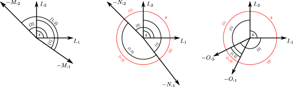
Figure 3: Complementary cones of the matrices $M$, $N$ and $O$ in Example 16, depicted by black arcs. The cones generated by $C_{\bar{N}}(\alpha)$ and $C_{\bar{O}}(\alpha)$ are depicted by red arcs. The matrices $M$ and $N$ are not equivalent, but $N$ and $O$ are, as their complementary cones have the same Boolean structure.

Note that

$${\bigcap}_{\alpha}\operatorname{pos}C_{M}(\alpha)=\operatorname{pos}C_{M}(\emptyset)\;.$$

Suppose, for the sake of argument, that there exists a bijection $g:\mathcal{G}_{M}\to\mathcal{G}_{N}$ that extends to an isomorphism $h:\mathcal{F}_{M}\to\mathcal{F}_{N}$. Then,

$$h\left({\bigcap}_{\alpha}\operatorname{pos}C_{M}(\alpha)\right) =h\left(\operatorname{pos}C_{M}(\emptyset)\right)$$

$${\bigcap}_{\alpha}\operatorname{pos}C_{N}(\hat{\beta}(\alpha)) =\operatorname{pos}C_{N}(\hat{\beta}(\emptyset))$$

for some bijection $\hat{\beta}$. However, note that the intersection of all the complementary cones generated by $N$ is no longer a cone. This is a contradiction, from which we conclude that such a $g$ cannot exist and that, by Remark 15, $M$ and $N$ are not equivalent. This is intuitively clear since, depending on the location of $q$, there can be none, two, or four solutions to the LCP $(M,q)$; whereas, depending on the location of $r$ there can be either one or three solutions to the LCP $(N,r)$.

Although $N$ and $O$ are fairly ‘distant’ from each other, they are LCP equivalent. To see this, consider the matrices

$$\bar{N}=\begin{bmatrix}N_{\boldsymbol{\cdot}2}&N_{\boldsymbol{\cdot}1}\end{bmatrix}\quad\text{and}\quad\bar{O}=\begin{bmatrix}O_{\boldsymbol{\cdot}2}&O_{\boldsymbol{\cdot}1}\end{bmatrix}\;.$$

It is lengthy but straight forward to verify that the mapping $\varphi:\mathbb{R}^{2}\to\mathbb{R}^{2}$, given by

$$\varphi(y^{\prime})=C_{\bar{N}}(\hat{\gamma}(\alpha))\cdot C_{\bar{O}}^{-1}(\alpha)\cdot y^{\prime}\;,\quad y^{\prime}\in\operatorname{pos}C_{\bar{O}}(\alpha)$$

with $\hat{\gamma}(\emptyset)=\{1,2\}$, $\hat{\gamma}(\{1\})=\{1\}$, $\hat{\gamma}(\{2\})=\{2\}$ and $\hat{\gamma}(\{1,2\})=\emptyset$, maps the cones $\operatorname{pos}C_{\bar{O}}(\alpha)$ to the cones $\operatorname{pos}C_{\bar{N}}(\hat{\gamma}(\alpha))$ (see Fig. 3). Clearly, $\varphi$ is a homeomorphism. Also, it induces the mapping $g:\mathcal{G}_{N}\to\mathcal{G}_{O}$ given by

$$g\left(\operatorname{pos}C_{N}(\alpha)\right)=\operatorname{pos}C_{O}(-\alpha)\;.$$

We have verified the conditions of Theorem 14.

In the example, $M$ and $N$ are not equivalent, even though they are ‘close’ to each other. This issue takes us to the following concept.

Definition 17.

A matrix $M\in\mathbb{R}^{n\times n}$ is said to be LCP stable if it is LCP equivalent to every matrix that is sufficiently close to it.

3.2 Classification of LCPs on the plane

The following results will provide a characterization of equivalence classes of stable matrices in $\mathbb{R}^{2\times 2}$.

Lemma 18.

Let $M\in\mathbb{R}^{2\times 2}$. If $M_{12},M_{21}\neq 0$ and $\det(M_{\alpha\alpha})\neq 0$, for all $\alpha\subseteq\{1,2\}$, then $M$ is stable.

Let $E_{M}=\begin{bmatrix}I&-M\end{bmatrix}$, let $A_{\alpha}$ with $\alpha\subseteq\{1,2\}$ be the connected components of $\mathbb{R}^{2}-\bigcup_{i=1}^{4}\operatorname{pos}E_{M\boldsymbol{\cdot}i}$, and note that $A_{\alpha}$ are (not necessarily convex) cones that partition $\mathbb{R}^{2}$, i.e., ${\bigcup}_{\alpha}\bar{A}_{\alpha}=\mathbb{R}^{2}$ and $A_{\alpha}\cap A_{\beta}=\emptyset$ for $\alpha\neq\beta$. For every index $\alpha$, define $G_{M}(\alpha)\in\mathbb{R}^{2\times 2}$ as the submatrix of $E_{M}$ such that

$$\operatorname{bdr}A_{\alpha}=\operatorname{pos}G_{M}(\alpha)_{\boldsymbol{\cdot}1}\cup\operatorname{pos}G_{M}(\alpha)_{\boldsymbol{\cdot}2}$$

and $|G_{M}(\alpha)|>0$. Let $M^{\prime}=M+\varepsilon\tilde{M}$ be a perturbation of $M$. The matrix $E_{M^{\prime}}$ varies smoothly as a function of $\varepsilon$. In particular, $M^{\prime}_{\boldsymbol{\cdot}i}\to M_{\boldsymbol{\cdot}i}$ as $\varepsilon\to 0$ (where the convergence is in some, and thus every, norm on $\mathbb{R}^{n}$).

Let $\varphi:\mathbb{R}^{2}\to\mathbb{R}^{2}$ be defined by

$$\varphi(y^{\prime})=G_{M}(\alpha)\cdot G_{M^{\prime}}^{-1}(\alpha)\cdot y^{\prime}\;,\quad y^{\prime}\in A^{\prime}_{\alpha}$$

with $G_{M^{\prime}}(\alpha)$ the $\varepsilon$-perturbation of $G_{M}(\alpha)$ such that $|G_{M^{\prime}}(\alpha)|>0$. Thus, $\varphi|_{A^{\prime}_{\alpha}}$, $\alpha\subseteq\{1,2\}$, is continuous and bijective. We now show that $\varphi$ is well-defined, continuous, and bijective at the cone boundaries, too. Let $A^{\prime}_{\alpha}$ and $A^{\prime}_{\beta}$ be two contiguous cones with common boundary $\operatorname{pos}E_{M^{\prime}\boldsymbol{\cdot}i}$. Note that, if $y^{\prime}\in A^{\prime}_{\alpha}\cap A^{\prime}_{\beta}$, then $y^{\prime}=\kappa E_{M^{\prime}\boldsymbol{\cdot}i}$ for some $\kappa>0$, so that

$$\varphi|_{A^{\prime}_{\alpha}}(y^{\prime})=\kappa E_{M^{\prime}\boldsymbol{\cdot}i}=\varphi|_{A_{\beta}}(y^{\prime})\;.$$

Thus $\varphi:\mathbb{R}^{2}\to\mathbb{R}^{2}$ is a homeomorphism. Moreover, since $\varphi(I_{\boldsymbol{\cdot}i})=I_{\boldsymbol{\cdot}i}$, $i=1,2$, and $\varphi(M^{\prime}_{\boldsymbol{\cdot}i})=M_{\boldsymbol{\cdot}i}$, $i=1,2$, it follows that $\varphi^{-1}(\operatorname{pos}C_{M}(\alpha))=\operatorname{pos}C_{M^{\prime}}(\alpha)$, that is, $\varphi^{-1}$ induces a bijection $g:\mathcal{G}_{M}\to\mathcal{G}_{M^{\prime}}$. Then Theorem 14 implies $M$ and $M^{\prime}$ are equivalent. ∎

Theorem 19.

Two matrices $M,N\in\mathbb{R}^{2\times 2}$ are equivalent if

$$M_{12}\cdot N_{12}>0,\ M_{21}\cdot N_{21}>0$$

and

$$\det(M_{\alpha\alpha})\cdot\det(N_{\alpha\alpha})>0\;,\quad\alpha\subseteq\left\{1,2\right\}\;.$$

Under the hypothesis of the theorem, $M_{t}:=(1-t)M+tN$ is stable for all $t\in[0,1]$, because $M_{t}$ satisfies the conditions of Lemma 18 for all $t\in[0,1]$. Thus, for all $t\in[0,1]$ there exists a neighborhood $U_{t}$ of $t$ in $[0,1]$ such that $M_{t}\sim M_{t^{\prime}}$ for all $t^{\prime}\in U_{t}$. Because $[0,1]$ is compact, we can cover it with a finite number of $U_{t}$’s, say, for $t_{0}<t_{1}<\cdots<t_{n}$, with $0\in U_{t_{0}}$ and $1\in U_{t_{n}}$. Let $\tau_{i}\in U_{t_{i-1}}\cap U_{t_{i}}$, $i=1,\ldots,n$. Then $M=M_{0}\sim M_{\tau_{1}}\sim M_{\tau_{2}}\sim\cdots\sim M_{\tau_{n}}\sim M_{1}=N$. ∎

Corollary 20.

Let $M\in\mathbb{R}^{2\times 2}$ with $\det(M_{\alpha\alpha})=0$ for some $\alpha\subseteq\{1,2\}$, then $M$ is not stable.

Recalling that non-singular matrices are dense, there exists $M^{\prime}$ arbitrarily close to $M$ such that $\det(M^{\prime}_{\alpha\alpha})\neq 0$ for all $\alpha\subseteq\{1,2\}$. Then, any bijection $g:\mathcal{G}_{M}\to\mathcal{G}_{M^{\prime}}$ cannot be induced by a homeomorphism $\varphi^{-1}$. If it was, $\varphi^{-1}$ would map an empty-interior complementarity cone to a non-empty interior complementarity cone, a contradiction. It follows by Theorem 14 that $M$ cannot be stable. ∎

The results of this section provides a list of “normal forms” to explore equivalence classes of stable matrices in $\mathbb{R}^{2\times 2}$. The matrices

$$M_{\delta}=\begin{bmatrix}\delta_{1}&\delta_{3}\\ -\delta_{3}(2\delta_{0}-\delta_{1}\delta_{2})&\delta_{2}\end{bmatrix}$$

and

$$N_{\delta}=\begin{bmatrix}\delta_{1}&\delta_{3}\\ -\delta_{3}(0.5\delta_{0}-\delta_{1}\delta_{2})&\delta_{2}\;,\end{bmatrix}$$

with $\delta_{i}\in\{-1,1\}$, $i=0,\ldots,3$ span all possible sign combinations in the statement of Theorem 19. Thus, any stable matrix satisfying the condition of the theorem is equivalent to $M_{\delta}$, for some combination of $\delta_{i}\in\{-1,1\}$, $i=0,\ldots,4$. By varying the parameters of $M_{\delta}$, we can thus construct an explicit list of equivalence classes of stable bidimensional matrices. The constructed list might not be exhaustive, but by Corollary 20 what is left out from this classification is the zero-measure set of matrices satisfying $\det(M_{\alpha\alpha})\neq 0$, for all $\alpha\subseteq\{1,2\}$, but $M_{12}M_{21}=0$. Stability and equivalence class of matrices in this zero-measure set are assessed a posteriori on a case-by-case basis in the normal form matrix

$$O_{\delta}=\begin{bmatrix}\delta_{1}&\delta_{3}\\ \delta_{4}&\delta_{2}\end{bmatrix}$$

with $\delta_{1},\delta_{2}\in\{-1,1\}$ and $\delta_{3},\delta_{4}\in\{-1,0,1\}$, $\delta_{3}\delta_{4}=0$.

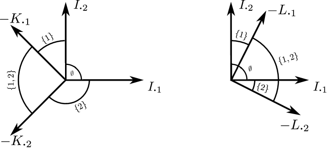
Figure 4: Complementary cones of the matrices $K$ (left) and $L$ (right) defined in (15), depicted by black arcs.

After studying the cone structure of each of these matrices, we conclude that there are only four classes of LCP stable matrices in $\mathbb{R}^{2\times 2}$. Representative members of two different classes are the matrices $M$ and $N$, defined in Example 16. Two more representative matrices are

$$K=\begin{bmatrix}1&1\\ -1&1\end{bmatrix}\quad\text{and}\quad L=\begin{bmatrix}-0.5&-1\\ -1&0.5\end{bmatrix}\;.$$ (15)

Since $\mathcal{G}_{K}$ partitions $\mathbb{R}^{2}$ (see Fig. 4), the LCP $(K,q)$ has a unique solution for every $q$. A matrix with this property is called a $P$-matrix (Cottle et al., 2009). The complementary cones of $L$ are also shown in Fig. 4. Depending on $q$, the LCP $(L,q)$ may either have two or no solutions.

3.3 Bifurcation realization via LCP interconnection

The strong link between piecewise linear functions and LCP’s, pointed out in Proposition 2, motivates us to restrict ourselves to piecewise linear paths through cone configurations. In this setting, the path itself can be generated from the solution set of another LCP (Eaves and Lemke, 1981; Garcia et al., 1983). This approach naturally leads us towards an interconnection framework reminiscent of circuit theory, in the sense that an intricate high-dimensional LCP is treated as the result of the interconnection of simpler LCP’s. Proceeding in this way we prove that, by selecting appropriate inputs and outputs, the feedback interconnection of LCPs is again an LCP. Afterwards, we use this decomposition approach to obtain the unfoldings of the pitchfork singularity.

We start by considering two linear complementarity problems in their $z$-coordinates, that is,

$$\text{LCP}(M_{k},\bar{q}_{k}):\begin{cases}w_{k}=M_{k}z_{k}+\bar{q}_{k}\\ \mathbb{R}_{+}^{n_{k}}\ni w_{k}\perp z_{k}\in\mathbb{R}_{+}^{n_{k}}\end{cases}\;,$$

where $M_{k}\in\mathbb{R}^{n_{k}\times n_{k}}$ and $\bar{q}_{k}\in\mathbb{R}^{n_{k}}$, for $k\in\{a,b\}$. Let $z_{k}\in\mathbb{R}^{n_{k}}$ be the output of the $k$-th LCP and let $\bar{q}_{k}\in\mathbb{R}^{n_{k}}$ take the role of input. Additionally, consider the interconnection rule

$$\bar{q}_{a}=H_{a}z_{b}+\bar{\theta}_{a}\;,\quad\bar{q}_{b}=H_{b}z_{a}+\bar{\theta}_{b}\;,$$ (16)

where $H_{a}\in\mathbb{R}^{n_{a}\times n_{b}}$, $H_{b}\in\mathbb{R}^{n_{b}\times n_{a}}$ and $\bar{\theta}_{k}\in\mathbb{R}^{n_{k}}$ are additional inputs available for further interconnection. With this convention we have the following result.

Proposition 21.

The interconnection of linear complementarity problems under the pattern (16) is again a linear complementarity problem.

The interconnection of two LCPs under the pattern (16) yields,

$$\begin{cases}\begin{bmatrix}w_{a}\\ w_{b}\end{bmatrix}=\begin{bmatrix}M_{a}&H_{a}\\ H_{b}&M_{b}\end{bmatrix}\begin{bmatrix}z_{a}\\ z_{b}\end{bmatrix}+\begin{bmatrix}\bar{\theta}_{a}\\ \bar{\theta}_{b}\end{bmatrix}\\ \mathbb{R}_{+}^{n_{a}+n_{b}}\ni\begin{bmatrix}w_{a}\\ w_{b}\end{bmatrix}\perp\begin{bmatrix}z_{a}\\ z_{b}\end{bmatrix}\in\mathbb{R}_{+}^{n_{a}+n_{b}}\end{cases}\;.$$ (17)

The conclusion follows directly from (17), which is an LCP of dimension $n_{a}+n_{b}$ with extended input $\begin{bmatrix}\bar{\theta}_{a}&\bar{\theta}_{b}\end{bmatrix}^{\top}$ and extended output $\begin{bmatrix}z_{a}&z_{b}\end{bmatrix}^{\top}$. ∎ Note that, in contrast to the framework of dynamical systems, we are studying static relations that may be set-valued. Thus, the conditions for well-posedness of (17) are more relaxed in comparison with their smooth counterpart.

3.4 Realization of some non-smooth bifurcations and their unfolding: A non-smooth pleat

Let us consider the class of LCPs represented by the matrix $O$ in Fig. 3. This class gives rise to the non-smooth pleat shown in Fig. 5. The pleat is given by

$$\left\{\begin{bmatrix}y_{1}&y_{2}&x_{1}\end{bmatrix}^{\top}\in\mathbb{R}^{3}\mid\exists\;x_{2}\in\mathbb{R}\text{ such that }f_{O}(x)=y\right\}\;,$$

where $f_{O}:\mathbb{R}^{2}\to\mathbb{R}^{2}$ is the piecewise linear map defined in Proposition 2. It is worth to remark that the non-smooth pleat is stable in the sense that the matrix $O$ is LCP-stable.

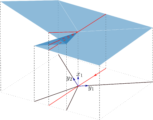
Figure 5: Non-smooth pleat, pitchfork path, and their projection to the plane $(y_{1},y_{2})$. The black lines on the plane are generators of complementary cones.

In complete analogy with the smooth case, see e.g. (Golubitsky and Schaeffer, 1985, Chapter III.12), one can recover a large family of bifurcations from the pleat by selecting appropriate paths through it. We illustrate this with the pitchfork singularity and its unfoldings, but it is also possible to obtain the hysteresis and the cusp singularities and their unfoldings by changing the path in a suitable way.

Concretely, let us consider the LCP $(M_{b},\bar{q}_{b})$ associated to the non-smooth pleat shown in Fig. 5 with matrix $M_{b}=2O$ and $O$ as in Example 16. In order to realize the path $\bar{q}_{b}$, we follow the interconnection approach described in the previous subsection. We consider the second LCP $(M_{a},\bar{q}_{a})$ with $M_{a}=1$ and path $\bar{q}_{a}(\lambda)=2\lambda-1$. The LCP $(M_{a},\bar{q}_{a})$ has a unique solution for every $\lambda\in\mathbb{R}$ which is computed easily as

$$z_{a}(\lambda)=\begin{cases}0,&\lambda<\frac{1}{2}\\ 2\lambda-1,&\frac{1}{2}\leq\lambda\end{cases}\;.$$ (18)

We thus set the path $\bar{q}_{b}(\lambda)$ as

$$\bar{q}_{b}(\lambda)=R_{s}\begin{bmatrix}z_{a}(\lambda)\\ \lambda\end{bmatrix}+\begin{bmatrix}\mu_{1}\\ \mu_{2}\end{bmatrix}\;,$$

where $R_{s}$ is a rotation matrix, $s$ is the angle of rotation and the parameters $\mu_{1},\mu_{2}$ are extra degrees of freedom that will allow us to change the path $\bar{q}_{b}(\lambda)$ on the pleat. Equivalently, the resulting LCP can be seen as the interconnection between LCP $(M_{a},\bar{q}_{a})$ and LCP $(M_{b},\bar{q}_{b})$ under the interconnection rule (16) with

$$H_{a} =0\;, H_{b} =\begin{bmatrix}\cos s\\ \sin s\end{bmatrix}\;,$$

$$\bar{\theta}_{a} =\mu_{1}-\lambda\sin s\;, \bar{\theta}_{b} =\mu_{2}+\lambda\cos s\;.$$

Let us fix $s=\frac{10}{9}\pi$. By varying the parameters $\mu_{1}$ and $\mu_{2}$ we are able to displace the path $\bar{q}_{b}(\lambda)$ on the pleat whose projection onto the plane is depicted in Fig. 6 for different values of the vector $\mu$.

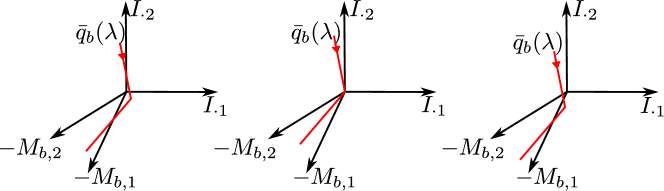
Figure 6: A sample of paths to recover the pitchfork singularity and its unfoldings.

The associated bifurcation diagrams to the paths on Fig. 6 are shown in Fig. 7. Note that the central path in Fig. 6 produces the pitchfork organizing center, whereas perturbations of this path lead to any of the left or right-hand side diagrams.

Figure 7: The pitchfork singularity and its unfoldings, obtained from the paths depicted in Fig. 6.

4 Discussion and future directions

We have presented a notion of global equivalence between LCPs that allows us to make a classification of this problems in the planar case. In addition, an interconnection approach for the realization of non-smooth bifurcations was presented. These tools are thought to be handful for many applications, as for instance, the analysis and design of neuromorphic circuits (Castaños and Franci, 2017), the study of economic equilibria in competitive markets (Nagurney, 1999), and the analysis of elastic-plastic structures in engineering (Pang et al., 1979), just to name a few. This work also opens the path towards the analysis of behaviors in dynamical linear complementarity systems (van der Schaft and Schumacher, 1998).

References

- Acary et al. (2011) Acary, V., Bonnefon, O., and Brogliato, B. (2011). Nonsmooth modeling and simulation for switched circuits. Lecture Notes in Electrical Engineering. Springer.
- Arnold et al. (1985) Arnold, V.I., Varchenko, A.N., and Gusein-Zade, S.M. (1985). Singularities of Differentiable Maps, volume 1. Birkhäuser.
- Brogliato (1999) Brogliato, B. (1999). Nonsmooth mechanics: models, dynamics and control. Springer-Verlag, London, second edition.
- Castaños and Franci (2017) Castaños, F. and Franci, A. (2017). Implementing robust neuromodulation in neuromorphic circuits. Neurocomputing, 233, 3–13.
- Clarke (1990) Clarke, F. (1990). Optimization and nonsmooth analysis. Society for Industrial and Applied Mathematics.
- Cottle et al. (2009) Cottle, R.W., Pang, J.S., and Stone, R.E. (2009). The Linear Complementarity Problem. Classics in Applied Mathematics. Society for Industrial and Applied Mathematics.
- Danao (1994) Danao, R.A. (1994). Q-matrices and boundedness of solutions to linear complementarity problems. Journal of Optimization Theory and Applications, 83(2), 321–332.
- Di Bernardo et al. (2008) Di Bernardo, M., Budd, C.J., Champneys, A.R., Kowalczyk, P., Nordmark, A.B., Tost, G.O., and Piiroinen, P.T. (2008). Bifurcations in nonsmooth dynamical systems. SIAM review, 50(4), 629–701.
- Dontchev and Rockafellar (2014) Dontchev, A.L. and Rockafellar, R.T. (2014). Implicit Functions and Solution Mappings. Springer, New York, second edition.
- Eaves and Lemke (1981) Eaves, B.C. and Lemke, C.E. (1981). Equivalence of LCP and PLS. Mathematics of Operation Research, 6(4), 475–484.
- Garcia et al. (1983) Garcia, C.B., Gould, F.J., and Turnbull, T.R. (1983). Relations between PL maps, complementary cones, and degree in linear complementarity problems. In Homotopy Methods and Global Convergence, 91–144. Plenum Publishing Corporation.
- Givant and Halmos (2009) Givant, S. and Halmos, P.R. (2009). Introduction to Boolean Algebras. Springer-Verlag, New York.
- Golubitsky and Schaeffer (1985) Golubitsky, M. and Schaeffer, D. (1985). Singularities and Groups in Bifurcation Theory, volume I of Applied Mathematical Sciences. Springer, New York.
- Leenaerts and Bokhoven (1998) Leenaerts, D.M. and Bokhoven, W.M.G. (1998). Piecewise linear modeling and analysis. Kluwer Academic. Springer, New York.
- Leine and Nijmeijer (2004) Leine, R.I. and Nijmeijer, H. (2004). Dynamics and bifurcations on non-smooth mechanical systems. Springer, Berlin.
- Murty (1988) Murty, K.G. (1988). Linear complementarity, linear and nonlinear programming. Helderman Verlag, Berlin.
- Murty (1972) Murty, K.G. (1972). On the number of solutions to the complementarity problem and spanning properties of complementary cones. Linear Algebra and Its Applications, 5(1), 65–108.
- Nagurney (1999) Nagurney, A. (1999). Network economics: A variational inequality approach. Advances in Computational Economics. Springer-Science+Business Media.
- Pang et al. (1979) Pang, J., Kaneko, I., and Hallman, W. (1979). On the solution of some (parametric) linear complementarity problems with applications to portfolio selection, structural engineering and actuarial graduation. Mathematical Programming, 16, 325 – 347.
- Sikorski (1969) Sikorski, R. (1969). Boolean Algebras. Springer-Verlag, Berlin, Germany.
- Simpson (2010) Simpson, D.J.W. (2010). Bifurcations in piecewise-smooth continuous systems. World Scientific, Singapore.
- van der Schaft and Schumacher (1998) van der Schaft, A.J. and Schumacher, J. (1998). Complementarity modeling of hybrid systems. IEEE Trans. Autom. Control, 43, 483 – 490.