An Asymptotically F-Distributed Chow Test in the Presence of Heteroscedasticity and Autocorrelation††thanks: We thank Derrick H. Sun for excellent research assistance.
Abstract
This study proposes a simple, trustworthy Chow test in the presence of heteroscedasticity and autocorrelation. The test is based on a series heteroscedasticity and autocorrelation robust variance estimator with judiciously crafted basis functions. Like the Chow test in a classical normal linear regression, the proposed test employs the standard F distribution as the reference distribution, which is justified under fixed-smoothing asymptotics. Monte Carlo simulations show that the null rejection probability of the asymptotic F test is closer to the nominal level than that of the chi-square test.
Keywords: Chow Test, F Distribution, Heteroscedasticity and Autocorrelation, Structural Break.
1 Introduction
For predictive modeling and policy analysis using time series data, it is important to check whether a structural relationship is stable over time. The Chow, (1960) test is designed to test whether a break takes place at a given period in an otherwise stable relationship. The test is widely used in empirical applications and has been included in standard econometric textbooks. This paper considers the Chow test in the presence of heteroscedasticity and autocorrelation. There is ample evidence that the Chow test can have very large size distortions if heteroscedasticity and autocorrelation are not accounted for (e.g., Krämer, (1989) and Giles and Scott, (1992)). Even if we account for them using heteroscedasticity and autocorrelation robust (HAR) variance estimators (e.g., Newey and West, (1987) and Andrews, (1991)), the test can still over-reject the null hypothesis by a large margin if chi-square critical values are used111When the Chow test is performed on a single coefficient, normal critical values are typically used on the t statistic. For now, we focus only on the Wald-type Chow test for more than one coefficients so that chi-square critical values are used.. This is a general problem for any HAR inference, as the chi-square approximation ignores the often substantial finite sample randomness of the HAR variance estimator. To address this problem, the recent literature has developed a new type of asymptotics known as fixed-smoothing asymptotics (see, e.g., Kiefer and Vogelsang, 2002a ; Kiefer and Vogelsang, 2002b ; Kiefer and Vogelsang, (2005) for early seminal contributions). It is now well known that the fixed-smoothing asymptotic approximation is more accurate than the chi-square approximation. This has been confirmed by ample simulation evidence and supported by higher-order asymptotic theory in Jansson, (2004) and Sun et al., (2008).
In this study, we employ the series HAR variance estimator to implement the Chow test in a time series regression where the regressors and regression errors are autocorrelated. This type of HAR variance estimator is the series counterpart of the kernel HAR variance estimator. The advantage of using the series HAR variance estimator is that we can design the basis functions so that the fixed-smoothing asymptotic distribution is the standard F distribution. This is in contrast to commonly used kernel HAR variance estimators where the fixed-smoothing asymptotic distributions are nonstandard and critical values have to be simulated222In the series case, fixed-smoothing asymptotics holds the number of basis functions fixed as the sample size increases. In the kernel case, fixed-smoothing asymptotics holds the truncation lag parameter fixed at a certain proportion of the sample size..
To establish the asymptotic F theory for the Chow test under fixed-smoothing asymptotics, we have to transform the usual orthonormal bases such as sine and cosine bases using the Gram–Schmidt orthonormalization. This is because, unlike the HAR inference in a regression with stationary regressors and regression errors, using the usual bases as in Sun, (2013) does not lead to a standard fixed-smoothing asymptotic distribution, since the regressors in the regression for the structural break test are identically zero before or after the break point and are thus not stationary. The Gram–Schmidt orthonormalization ensures that the transformed bases are orthonormal with respect to a special inner product that is built into the problem under consideration. The asymptotic F test is very convenient to use, as the F critical values are readily available from standard statistical tables and programming environments.
Monte Carlo simulation experiments show that the F test based on the transformed Fourier bases is as accurate as the nonstandard test based on the usual Fourier bases. The F test and nonstandard test have the same size-adjusted power as the corresponding chi-square tests but much more accurate size. Given its convenience, competitive power, and higher size accuracy, we recommend the F test for practical use.
Our F test theory generalizes the classical Chow test in a linear normal regression where the F distribution is the exact finite sample distribution. The main departures are that we do not make the normality assumption and that we allow for heteroscedasticity and autocorrelation of unknown forms. Without restrictive assumptions such as normality and strict exogeneity, it is in general not possible to obtain the exact finite sample distribution. Instead, we employ the fixed-smoothing asymptotics to show that the Wald statistic is asymptotically F distributed.
This study contributes to the asymptotic F test theory in the HAR literature. The asymptotic F theory has been developed in a number of papers including Sun, (2011); Sun and Kim, (2012); Sun, (2013); Hwang and Sun, (2017); Lazarus et al., (2018); Liu and Sun, (2019); Wang and Sun, (2019); Martínez-Iriarte et al., (2019). However, none of these studies considers the case where the regressors take the special form of nonstationarity as we consider here. Cho and Vogelsang, (2017) consider fixed-b asymptotics for testing structural breaks, but they consider only kernel HAR variance estimators. As a result, the fixed-smoothing asymptotic distributions they obtained are highly nonstandard.
The rest of this paper is organized as follows. Section 2 presents the basic setting and introduces the test statistics. Section 3 establishes the fixed-smoothing asymptotics of the F and t statistics. Section 4 develops asymptotically valid F and t tests. Section 5 extends the basic regression model to include other covariates whose coefficients are known to be stable over time. Section 6 reports the simulation evidence. The last section concludes. Proofs are given in the appendix.
2 Basic Setting and Test Statistics
Given the time series observations we consider the model
for where the unobserved satisfies In the above, is a known parameter in so that is the period where the structural break may take place. The effects of on before and after the break are and respectively. We allow to exhibit autocorrelation of unknown forms. In particular, we allow to be heteroskedastic so that is a nontrivial function of
We are interested in testing the null of : against the alternative for some matrix When is the identity matrix, we aim at testing whether is equal to For the moment, we consider the case that all coefficients are subject to a possible break. In Section 5, we consider the case that some of the coefficients are known to be time invariant.
Let
Note that both and are nonstationary. The form of the nonstationarity makes the problem at hand unique. Let and Then
and the hypotheses of interest become and for
Denote , and We estimate by OLS:
The OLS estimator satisfies
where
and is a matrix of zeros. To make inferences on such as testing whether is zero, we need to estimate the variance of To this end, we first construct the residual which serves as an estimate for Given a set of basis functions we then construct the series estimator of the variance as
where, for a column vector is the outer product of that is, The asymptotic variance of is then estimated by
The Wald statistic for testing against is
When and we test against a one-sided alternative, say, , we can construct the t statistic:
The forms of the F and t statistics are standard.
3 Fixed-smoothing Asymptotic Distributions
To establish the asymptotic distributions of and we maintain the following three assumptions:
Assumption 3.1
uniformly over and is invertible.
Assumption 3.2
for where is the long run variance of and is an standard Brownian process.
Assumption 3.3
The basis functions , are piecewise monotonic and piecewise continuously differentiable.
Note that and are the average changes of the Brownian motion over the intervals and respectively. Lemma 3.1 shows that and are (matrix) proportional to the average changes. Given the independence of these changes over any non-overlapping intervals, and are asymptotically independent.
Note that can be regarded as an average of over the interval Similarly, can be regarded as an average of over the interval So and are the demeaned versions of over the intervals and respectively.
Using Lemma 3.1, we can prove our main theorem below.
Like the finite sample distributions, the limiting distributions of and depend on and the number and form of the basis functions. This is an attractive feature of the fixed-smoothing approximations, as they capture the effects of all these factors. More importantly, the fixed-smoothing approximations capture the randomness of the HAR variance estimator, which clearly affects the finite sample distributions of and This is why the fixed-smoothing asymptotic approximations are more accurate than the chi-square or normal approximations.
4 Asymptotic F and t Theory
The limiting distributions and in Theorem 3.1 are pivotal but nonstandard. We can approximate the nonstandard distributions using a chi-square or t distribution. We can also design a new set of basis functions so that and become the standard F and t distributions after some multiplicative adjustment.
4.1 Chi-square and normal approximations
Define
Then
and so
As a result,
where
When is relatively large, it is reasonable to approximate by its mean:
With such an approximation, we have
where ‘’ signifies distributional approximations. As a result, we can employ the following approximations:
| (3) | ||||
| (4) |
where is the finite sample version of given by
| (5) |
It is important to point out that the chi-square and normal approximations are not based on the original Wald and t statistics but rather on their modified versions and . To a great extent, the chi-square and normal approximations we propose here improve upon the conventional chi-square and normal approximations that are applied directly to the original Wald and t statistics.
Note that the chi-square distribution and standard normal distribution in (3) and (4) are not the asymptotic distributions of and for a fixed The fixed- asymptotic distributions are given by
| (6) | ||||
| (7) |
These follow directly from Theorem 3.1. The chi-square distribution and standard normal distribution are only approximations to the above nonstandard fixed-K asymptotic distributions.
4.2 Asymptotic F and t Theory
To obtain convenient fixed-K asymptotic approximations, we note that for each is normal. For each we have
So is independent of , In addition,
Therefore, if are orthonormal, then for are independent standard normals. In this case, is a quadratic form in a standard normal vector with an independent weighting matrix. After some adjustment, we can show that is equal to a standard F distribution and that converges to the F distribution. Similarly, converges to Student’s t distribution.
Proposition 4.1
This is a very convenient result, as the fixed-smoothing asymptotic approximations are standard distributions and there is no need to simulate critical values.
4.3 Designing the bases
To design the basis functions such that are orthonormal, we need the following lemma.
Lemma 4.1
Let be the Dirac delta function such that
Then
where
Let
be the transformed Brownian motion. Then we have
and
Therefore, can be regarded as the covariance kernel function for the transformed Brownian motion.
To design the basis functions such that are orthonormal on we require that be orthonormal with respect to the covariance kernel function that is,
| (8) |
This can be achieved by applying the Gram–Schmidt orthonormalization to any set of basis functions on . The chart below illustrates the procedure:
| GS | ||
In the above, is the initial set of basis functions, and is the Gram-Schmidt orthonormalized set. “” and “” reflect the effect of the estimation error in estimating had we known we would have used the true instead of in constructing the variance estimator, and the key elements of the weighting matrix in (1) in Theorem 3.1 would have been instead of The Gram-Schmidt orthonormalization ensures that are orthonormal with respect to the covariance kernel In view of
we have: are orthonormal on
If we use in constructing the variance estimator, then
for because are orthonormal on Moreover, for is independent of Therefore, the asymptotic F theory in Proposition 4.1 holds. Similarly, the asymptotic t theory holds.
Instead of searching for the basis functions that satisfy (8), we search for their discrete versions: the basis vectors. For each basis function the corresponding basis vector is defined as
Let be the matrix whose -th element is equal to
By definition, is symmetric and positive-definite. It is the discrete version of For any two vectors , we define the inner product
| (9) |
Then the discrete analogue of (8) is
| (10) |
Given any basis vectors we now apply the Gram–Schmidt orthonormalization via the Cholesky decomposition. Let be the matrix of basis vectors. Let be the upper triangular factor in the Cholesky decomposition of such that Define
We then have
That is, the columns of the matrix satisfy the conditions in (10).
Note that the -th element of satisfies
This implies that converges to the upper triangular factor of the Cholesky decomposition of var As a result, every transformed basis vector is approximately equal to a linear combination of the original basis vectors. The implied basis functions are thus equal to linear combinations of the original basis functions. Therefore, if Assumption 3.3 holds for the original basis functions, it also holds for the transformed basis functions. It then follows that Proposition 4.1 holds when are used as the basis vectors in constructing the asymptotic variance estimator. More specifically, if we estimate by
where is the -th element of the vector then the asymptotic F and t results in Proposition 4.1 hold.
5 The Chow Test in the presence of time-invariant effects
Suppose there is another covariate vector whose effect on does not change over time so that we have the model:
Let and Then
The OLS estimator of is now
Let and Define
The Wald statistic for testing against takes the same form as before:
When we construct the t statistic:
To establish the asymptotic distributions of and we maintain the two assumptions below, which are analogous to Assumptions 3.1 and 3.2.
Assumption 5.1
uniformly over for a invertible matrix .
Assumption 5.2
for where is the long run variance of the process and is an standard Brownian process.
We partition and according to
where and
6 Simulation Evidence
In this section, we investigate the finite sample properties of the proposed F test. We consider the linear regression model with and The regressor follows an AR(1) process, and the error follows an independent AR(1) or ARMA(1,1) process. That is,
where both and are iid and are independent of Note that the AR parameter is the same for and
We consider the sample sizes , and We let Without the loss of generality, we set and under the null. We consider testing against so that .
We consider two pairs of different tests, both of which are based on the series variance estimators. The first pair uses the (usual) Fourier bases
| (11) |
Each test in this pair is based on the same test statistic defined in (3) but uses different reference distributions. The first test uses the chi-square approximation () while the second test uses the nonstandard fixed-smoothing approximation given in (6). We refer to the two tests as “ Fourier Bases” and “ Fourier Bases,” respectively. The nonstandard critical values are simulated. We approximate the standard Brownian motion in the nonstandard distribution using scaled partial sums of 1000 iid random variables. To compute the nonstandard critical values, we use 10,000 simulation replications.
The second pair of tests uses the transformed Fourier bases via the Gram–Schmidt orthogonalization given in Section 4.3. Each of the two tests in this pair is based on the same test statistic defined in Proposition 4.1. The first test uses the standard F approximation, and the second test uses the rescaled chi-square distribution Equivalently, the second test in this pair employs the test statistic and the standard chi-square approximation (). We refer to the two tests as “ Transformed Bases” and “ Transformed Bases,” respectively. The chi-square test in the second pair is used to illustrate the effectiveness of the F approximation in reducing the size distortion.
The nominal level of all tests is The number of simulation replications is 10,000. Figures 1 and 2 report the null rejection probability for each test for the sample sizes and when and follow independent AR(1) processes with the same AR parameter Several patterns emerge from these two figures:
-
•
Regardless of the bases used, the chi-square tests over-reject the null by a large margin, especially when is small.
-
•
Regardless of the bases used, the nonstandard test and F test are much more accurate than the chi-square tests.
-
•
For each given value of the null rejection probabilities of the nonstandard test and F test are close to each other. This shows that, in terms of size accuracy, using the F approximation (when the transformed Fourier bases are employed) is as good as using the nonstandard approximation (when the Fourier bases are employed). However, the F approximation is more convenient to use and, hence, is preferred.
-
•
For each given value of the null rejection probabilities of the two chi-square tests are close to each other, although the one based on the transformed Fourier bases is somewhat more accurate. This shows that the bases do not have a large effect on the quality of the chi-square approximation.
-
•
The nonstandard test and standard F test can still have quite some size distortion if is large and the regressor and error processes are persistent. The size distortion comes from the bias of the variance estimator. When is large, we take an average over a frequency window that is too large when the processes are highly persistent, that is, when the spectral density of is not very flat at the origin. So, it is important to use a data-driven to obtain an accurate test in practice.
-
•
Comparing the two figures, we see that the size distortion of every test becomes smaller when the sample size is larger.
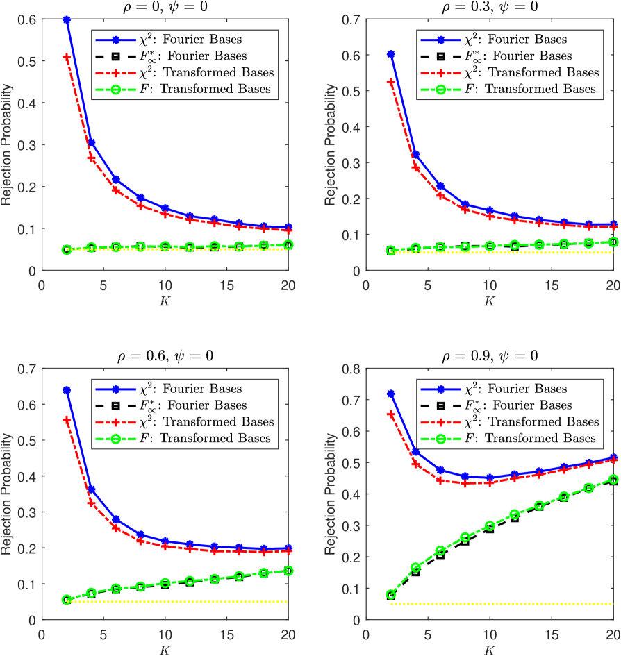
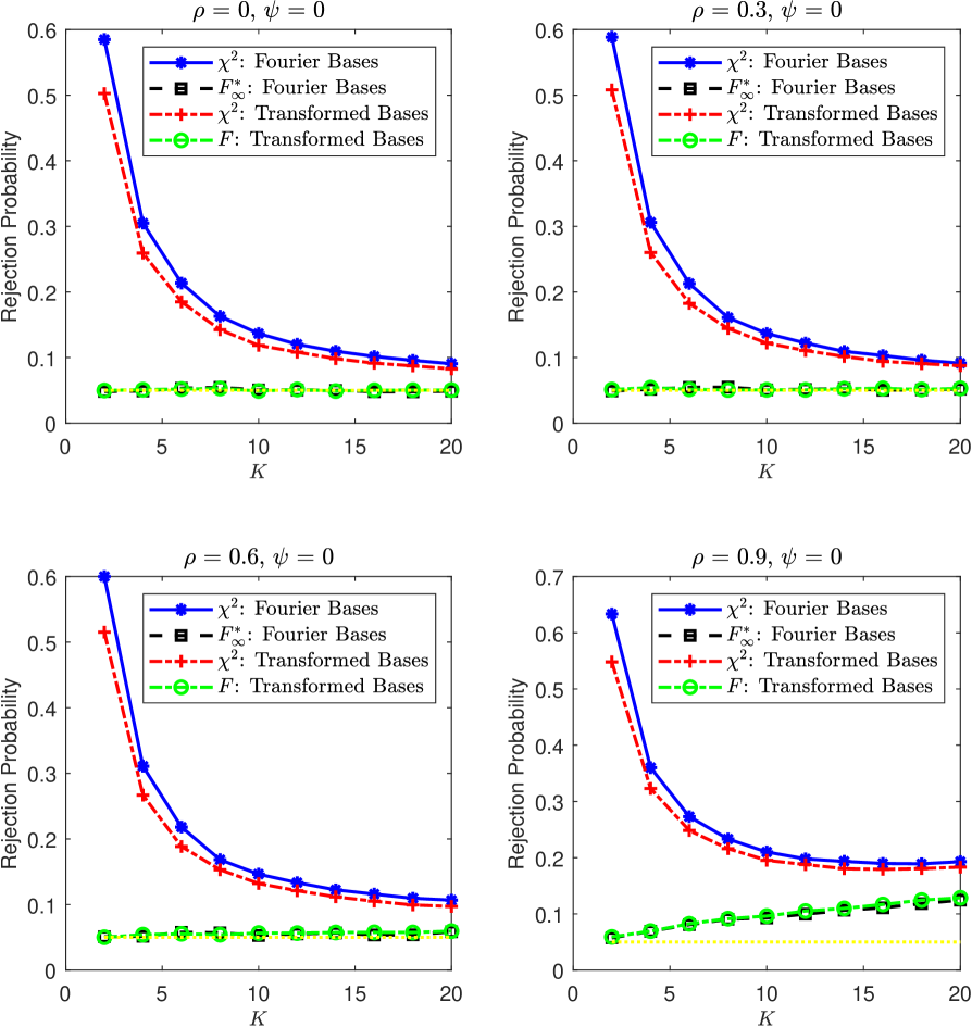
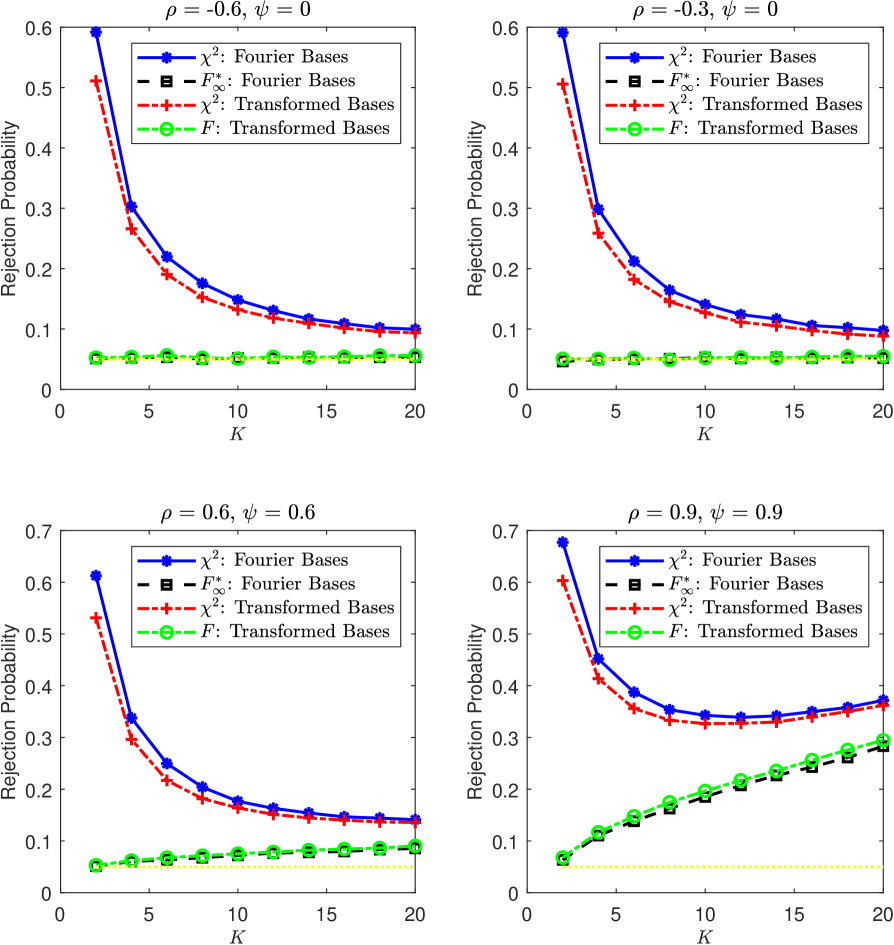
Figure 3 reports the null rejection probabilities when the sample size is and when the error process may have an MA component and the AR parameter may be negative. As in Figures 1 and 2, the same patterns emerge.
Next, we consider the size properties of the tests with a data-driven Note that
where Then
where So can be viewed as the series variance estimator of the long run variance of We can follow Phillips, (2005) and choose to minimize the mean square error (MSE) of We fit a VAR(1) model to and use the fitted model to compute the data-driven MSE-optimal
Table 1 reports the null rejection probabilities and the average values of used with data-driven choice of for different sample sizes. The qualitative observations from Figures 1– 3 continue to hold with the data-driven In particular, the nonstandard test and standard F test are more accurate than the corresponding chi-square tests, especially when the latter have large positive size distortion. The null rejection probabilities of the nonstandard test and the standard F test are close to each other. Similarly, the null rejection probabilities of the two chi-square tests are close to each other. As expected, the average value of decreases with the persistence of the underlying processes. The higher the persistence, the smaller the average value, and the more effective the nonstandard test and standard F test in reducing the size distortion.
| : Fourier | 0.092 | 0.131 | 0.227 | 0.511 | 0.128 | 0.091 | 0.287 | 0.558 |
|---|---|---|---|---|---|---|---|---|
| : Fourier | 0.060 | 0.076 | 0.101 | 0.198 | 0.067 | 0.056 | 0.087 | 0.170 |
| : Transformed | 0.089 | 0.124 | 0.210 | 0.473 | 0.119 | 0.085 | 0.259 | 0.516 |
| : Transformed | 0.064 | 0.079 | 0.101 | 0.209 | 0.071 | 0.060 | 0.088 | 0.182 |
| Ave | 30.00 | 18.40 | 9.71 | 5.29 | 16.57 | 26.34 | 6.14 | 4.27 |
| : Fourier | 0.069 | 0.100 | 0.153 | 0.396 | 0.092 | 0.070 | 0.197 | 0.444 |
| : Fourier | 0.052 | 0.066 | 0.079 | 0.150 | 0.055 | 0.050 | 0.075 | 0.131 |
| : Transformed | 0.068 | 0.094 | 0.142 | 0.363 | 0.088 | 0.067 | 0.179 | 0.406 |
| : Transformed | 0.057 | 0.069 | 0.082 | 0.153 | 0.058 | 0.051 | 0.074 | 0.135 |
| Ave | 70 | 28.82 | 14.32 | 6.10 | 24.96 | 46.02 | 8.56 | 4.56 |
| : Fourier | 0.055 | 0.068 | 0.096 | 0.222 | 0.067 | 0.057 | 0.119 | 0.278 |
| : Fourier | 0.049 | 0.054 | 0.062 | 0.091 | 0.053 | 0.048 | 0.056 | 0.084 |
| : Transformed | 0.053 | 0.064 | 0.091 | 0.209 | 0.064 | 0.055 | 0.110 | 0.253 |
| : Transformed | 0.048 | 0.053 | 0.062 | 0.096 | 0.051 | 0.048 | 0.058 | 0.086 |
| Ave | 144.51 | 56.47 | 26.91 | 9.03 | 46.58 | 96.41 | 15.19 | 6.05 |
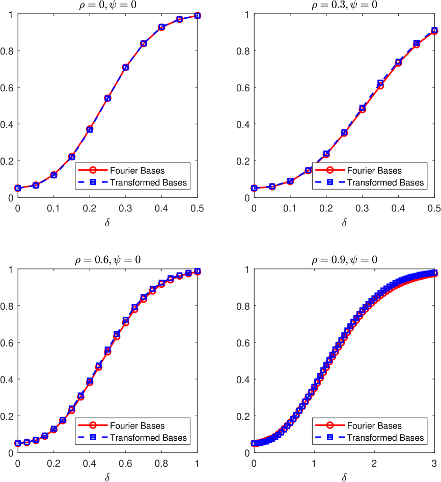
To simulate the power of the tests, we let and Figure 4 presents the size-adjusted power curves as functions of when the sample size is 200 and when both and follow AR(1) processes. The figure is representative of other cases. For the two tests in each pair, the size-adjusted powers are the same, as they are based on the same test statistic. Thus, we need only report two power curves: one for the usual Fourier bases and the other for the transformed Fourier bases. The basic message from Figure 4 is that the size-adjusted powers associated with the two sets of bases are very close to each other. This, coupled with its size accuracy and convenience to use, suggests that we use the F test in empirical applications.
7 Conclusion
This study proposes asymptotic F and t tests for structural breaks that are robust to heteroscedasticity and autocorrelation. The tests are based on a special series HAR variance estimator where the basis functions are crafted via the Gram–Schmidt orthonormalization. Monte Carlo simulations show that the F test is much more accurate than the corresponding chi-square test.
This study assumes that there is a single known break point. The asymptotic F and t theory can be extended to the case with multiple but known break points. The theory can also be extended to allow for a linear trend or other deterministic trends, but we need to redesign the basis functions. In principle, the tests based on series HAR variance estimation can be extended to accommodate the case with an unknown break point along the line of Cho and Vogelsang, (2017). All the basic ingredients have been established in the study. We only need to take the supremum (or other functionals) of the Wald or t statistic over as the test statistic. However, the convenient F approximation is lost, as the supremum of the standard distributions is not standard any more. Therefore, it is not clear whether there is still an advantage of using series HAR variance estimators rather than kernel HAR variance estimators.
8 Appendix of Proofs
For the second part of the lemma, we have
Now, it is not hard to show that under Assumption 3.3,
Hence,
Proof of Theorem 3.1. We have
Hence,
Also, under the null, we have
Therefore,
Using the fact that for a square and invertible matrix we have
The proof for the weak convergence of is similar and is omitted to save space.
Proof of Proposition 4.1. We prove the part for the Wald statistic only, as the proof for the t-statistic is similar. Given that are orthonormal on we have:
As a consequence,
the standard Wishart distribution with degrees of freedom So,
Note that are independent standard normal vectors. follows Hotelling’s distribution. Using the relationship between Hotelling’s distribution and the standard distribution, we have
It then follows that
Proof of Theorem 5.1. Part (a). Under Assumption 5.1, we have
Under Assumption 5.2, we have
where
Hence,
Using the matrix inverse formula
we have
where
Therefore,
| (12) |
and
Hence
Part (b) We have
where To find the limit of the first term in the above equation, we note that
where Therefore,
| (13) |
where we have used see (12).
Next,
| (16) | |||
| (19) | |||
| (22) | |||
| (27) |
So,
where we have used the fact that the last two terms in (27) pre-multiplied by are equal to zero.
It then follows that
As a consequence,
| (28) |
where
and
Plugging the above three terms and back into (28), we obtain:
| (29) |
where the last equality holds because
Part (c). We prove the case for only, as the proof for is similar. Using Parts (a) and (b), we have
Note that
for a invertible matrix such that Using this distributional equivalence, we have
as desired.
References
- Andrews, (1991) Andrews, D. W. K. (1991). Heteroskedasticity and autocorrelation consistent covariance matrix estimation. Econometrica, 59:817–858.
- Cho and Vogelsang, (2017) Cho, C.-K. and Vogelsang, T. J. (2017). Fixed-b inference for testing structural change in a time series regression. Econometrics, 5(1).
- Chow, (1960) Chow, G. C. (1960). Tests of equality between sets of coefficients in two linear regressions. Econometrica, 28(3):591–605.
- Giles and Scott, (1992) Giles, D. and Scott, M. (1992). Some consequences of using the Chow test in the context of autocorrelated disturbances. Economics Letters, 38(2):145 – 150.
- Hwang and Sun, (2017) Hwang, J. and Sun, Y. (2017). Asymptotic F and t tests in an efficient GMM setting. Journal of Econometrics, 198:277–295.
- Jansson, (2004) Jansson, M. (2004). On the error of rejection probability in simple autocorrelation robust tests. Econometrica, 72:937–946.
- (7) Kiefer, N. M. and Vogelsang, T. J. (2002a). Heteroskedasticity-autocorrelation robust testing using bandwidth equal to sample size. Econometric Theory, 18:1350–1366.
- (8) Kiefer, N. M. and Vogelsang, T. J. (2002b). Heteroskedasticity-autocorrelation robust standard errors using the Bartlett kernel without truncation. Econometrica, 70:2093–2095.
- Kiefer and Vogelsang, (2005) Kiefer, N. M. and Vogelsang, T. J. (2005). A new asymptotic theory for heteroskedasticity-autocorrelation robust tests. Econometric Theory, 21:1130–1164.
- Krämer, (1989) Krämer, W. (1989). The Robustness of the Chow Test to Autocorrelation among Disturbances, pages 45–52. in Statistical Analysis and Forecasting of Economic Structural Change, Springer.
- Lazarus et al., (2018) Lazarus, E., Lewis, D. J., Stock, J. H., and Watson, M. W. (2018). HAR inference: Recommendations for practice. Journal of Business & Economic Statistics, 36(4):541–559.
- Liu and Sun, (2019) Liu, C. and Sun, Y. (2019). A simple and trustworthy asymptotic t test in difference-in-differences regressions. Journal of Econometrics, 210(2):327 – 362.
- Martínez-Iriarte et al., (2019) Martínez-Iriarte, J., Sun, Y., and Wang, X. (2019). Asymptotic F tests under possibly weak identification. Working Paper, Department of Economics, UC San Diego.
- Newey and West, (1987) Newey, W. K. and West, K. D. (1987). A simple, positive semi-definite, heteroskedasticity and autocorrelation consistent covariance matrix. Econometrica, 55(3):703–708.
- Phillips, (2005) Phillips, P. C. B. (2005). HAC estimation by automated regression. Econometric Theory, 21(1):116–142.
- Sun, (2011) Sun, Y. (2011). Robust trend inference with series variance estimator and testing-optimal smoothing parameter. Journal of Econometrics, 164:345–366.
- Sun, (2013) Sun, Y. (2013). A heteroskedasticity and autocorrelation robust F test using orthonormal series variance estimator. Econometrics Journal, 16:1–26.
- Sun and Kim, (2012) Sun, Y. and Kim, M. S. (2012). Simple and powerful GMM over-identification tests with accurate size. Journal of Econometrics, 166:267–281.
- Sun et al., (2008) Sun, Y., Philips, P. C. B., and Jin, S. (2008). Optimal bandwidth selection in heteroskedasticity-autocorrelation robust testing. Econometrica, 76:175–194.
- Wang and Sun, (2019) Wang, X. and Sun, Y. (2019). An asymptotic F test for uncorrelatedness in the presence of time series dependence. Working Paper, Department of Economics, UC San Diego.