section0em3em subsection3em4em subsubsection7em4.5em

Optimal Experimental Design for Staggered Rollouts Optimal Experimental Design for Staggered Rollouts

Ruoxuan Xiong Department of Quantitative Theory and Methods, Emory University, ruoxuan.xiong@emory.edu Susan Athey Graduate School of Business, Stanford University, athey@stanford.edu Mohsen Bayati Graduate School of Business, Stanford University, bayati@stanford.edu Guido Imbens Graduate School of Business, Stanford University, imbens@stanford.edu

In this paper, we study the design and analysis of experiments conducted on a set of units over multiple time periods where the starting time of the treatment may vary by unit. The design problem involves selecting an initial treatment time for each unit in order to most precisely estimate both the instantaneous and cumulative effects of the treatment. We first consider non-adaptive experiments, where all treatment assignment decisions are made prior to the start of the experiment. For this case, we show that the optimization problem is generally NP-hard and we propose a near-optimal solution. Under this solution the fraction entering treatment each period is initially low, then high, and finally low again. Next, we study an adaptive experimental design problem, where both the decision to continue the experiment and treatment assignment decisions are updated after each period’s data is collected. For the adaptive case we propose a new algorithm, the Precision-Guided Adaptive Experiment (PGAE) algorithm, that addresses the challenges at both the design stage and at the stage of estimating treatment effects, ensuring valid post-experiment inference accounting for the adaptive nature of the design. Using realistic settings, we demonstrate that our proposed solutions can reduce the opportunity cost of the experiments by over 50%, compared to static design benchmarks.

Adaptive Experiments, Treatment Effect Estimation, Cumulative Effects, Panel Data, Dynamic Programming

1 Introduction

Large technology companies run tens of thousands of experiments (also known as A/B tests) per year to evaluate the impact of various decisions, new features, or products (Gupta et al. 2019). In many cases, outcomes are observed for multiple periods, where the units can change treatment status over time. We refer to these experiments as panel experiments; variants of these are sometimes referred to as experiments with staggered rollout or staggered adoption (Athey et al. 2021), or stepped wedge designs (Hemming et al. 2015).

Example 1.1 (Driver Experience)

Consider a ride-hailing platform that plans to test the impact of a new app feature that improves driver experience. They wish to run an experiment to estimate the effect of providing the app feature to all drivers. To avoid biases from interference between drivers it is useful to randomize at the city level where the starting time for the intervention may vary by city.

Example 1.2 (Public Health Intervention)

Consider a country that aims to measure the effect of a new public health intervention (e.g., encouraging the use of masks or social distancing policies) on the spread of an infectious disease (Abaluck et al. 2021). To account for spillovers experimentation should be performed at an aggregate level (e.g., cities). To facilitate the estimation of cumulative effects it is useful to vary the starting date.

The primary objective of this paper is to propose experimental designs to optimize the precision of post-experiment estimates of instantaneous and lagged effects of a treatment. To operationalize this, the experimenter commits in advance to an estimator which has a precision associated with each experimental design. The challenge is to find a design that optimizes this precision given the estimator.

We assume all units start in the control (no treatment) state at the initial time period. The design problem is to select, for each unit, the time period to begin treatment. We assume that units cannot switch back to control during the experiment, and thus remain treated once exposed to the treatment. This is a common setting. The treatment allocation time can vary across units, leading to a staggered treatment adoption or stepped wedge design.

1.1 Summary of Contributions

Non-adaptive experiments. We first study the design of non-adaptive experiments, where both the number of units and time periods and treatment decisions are determined prior to the start of the experiment. We focus on the properties of the generalized least squares (GLS) estimator. We consider a general version of feasible GLS to estimate instantaneous and lagged treatment effects from observed outcomes that can be non-stationary. The estimator determines the precision of estimated instantaneous and lagged effects. A linear combination of these precisions comprises the objective function for the experimental design problem. Finding the optimal solution is generally NP-hard. We provide the analytical optimality conditions for the design, and propose an algorithm to choose a treatment design based on the optimality conditions. The precision of our selected design approximates the optimal objective (best achievable precision) within a multiplicative factor of $1+O(1/N^{2})$ where $N$ is the number of units.

Our solution to the design problem of non-adaptive experiments has two prominent features. First, the fraction of treated units per time period takes an $S$-shaped curve; the treatment rolls out to units more slowly (over time) in the beginning and at the end, but rapidly in the middle, of the experiment. Second, the optimal design imposes this rollout pattern for each stratum, where strata are defined by groups with the same observed and estimated latent covariate values.

Adaptive experiments. Next we study the design of adaptive experiments, where the number of units is fixed, but the experiment can be terminated early and treatment assignment decisions can be adaptively made after each period’s data is collected. These experiments are useful when the pre-set duration is more than needed to attain a target precision of treatment effect estimates, and when treatment decisions cannot be optimally made ex ante. In our main contribution, we propose a new algorithm, the Precision-Guided Adaptive Experiment or PGAE algorithm, that adaptively terminates the experiment based on the estimated precision of the estimated treatment effect from partially observed results of the experiment. It employs dynamic programming to adaptively optimize the speed of treatment rollout in subsequent time periods. The resulting adaptive experiment achieves a target precision, using a shorter duration, or equivalently incurring a lower cost, than the non-adaptive experiment.

The adaptive nature of the experiment creates challenges arising from the fact that the outcomes and assignments that occur early in the experiment affect the treatment assignments to units later in the experiment. Thus, the treatment assignments are not independent of observed outcomes. We propose an estimation method based on sample splitting that ensures that the estimates obtained by PGAE are consistent and asymptotically converge to a normal distribution. An appealing property of the proposed estimation scheme we propose is that the final treatment effect estimation uses all of the data, incurring no efficiency loss compared to an oracle who would have access to the same design at the beginning of the experiment.

Finally, we illustrate the superior performance of our solutions, as compared to benchmarks, for non-adaptive and adaptive experiments through synthetic experiments based on four real data sets about flu occurrence rates, home medical visits, grocery expenditure, and Lending Club loans.

1.2 Related Literature

Our staggered rollout designs of panel experiments are related to a number of other experimental designs. They are most closely related to the stepped wedge designs in clinical trials (Brown and Lilford 2006). Stepped wedge designs sequentially roll out an intervention to clusters over several periods. Prior work on optimal stepped wedge design (Hussey and Hughes 2007, Hemming et al. 2015, Li et al. 2018) studies optimal treatment assignments of clusters under a linear mixed outcome model that has no observed or latent covariates and assumes constant treatment effect over time with instantaneous effects only. In contrast, we study the optimal design allowing treatment effects to vary over time (i.e., with instantaneous and lagged effects).

Related to our design, a few other designs proposed recently are suitable for studying time-varying treatment effects. One design is the synthetic control design for panel experiments where the design selects units to be treated, allocates treatment to all of them in a single period, and forms a synthetic treated and control unit for treatment effect estimation (Doudchenko et al. 2019, 2021, Abadie and Zhao 2021). Another design is the switchback design (Bojinov et al. 2023, Xiong et al. 2023) for a single experimental unit that can arbitrarily switch between treatment and control. In contrast to these two designs, our designs leverage variation in treatment times across units to increase power. The randomized designs proposed in Basse et al. (2023) also allow for cross-unit variation in treatment times, but they are studied under a different framework that minimizes the worst-case risk in randomization-based inference.

When interference between units is a concern, our design can be modified by following a conventional approach to avoid biases by aggregating units to a level that interference is no longer a problem. But we note a growing literature that directly tackles the biases using novel experimental design ideas, such as multiple randomization (Bajari et al. 2023, Johari et al. 2022) and designs that perturb treatments near equilibrium outcomes (Wager and Xu 2021). In contrast, our design, by abstracting away from interference, can be used to study the rich dynamics of cumulative effects over time.

Different from all the aforementioned designs, we additionally study the design and analysis of adaptive experiments. Our proposed PGAE algorithm consists of three components: adaptive treatment decisions, an experiment termination rule, and post-experiment inference. The adaptive treatment decision component relates to the literature on adaptive designs in sequential experiments (e.g., Efron (1971), Bhat et al. (2019), Glynn et al. (2020)), online learning and multi-armed bandits (e.g., Bubeck et al. (2012), Lattimore and Szepesvári (2020)). Distinct from this literature, we consider a panel setting, and our design choices allow for experiment termination and ensure that inference is manageable.

The experiment termination rule component is based on the precision of the treatment effect estimate. The precision-based termination rule has been used to obtain fixed-volume confidence sets from a sequence of independent random variables (Glynn and Whitt 1992a, b, Singham and Schruben 2012). We extend the use of this rule to the panel setting. Our proposed PGAE algorithm decides whether to terminate the experiment at every period, which is related to the sequential testing problem, considered by Siegmund (1985), Wald (2004), Bertsekas (2012), Johari et al. (2017), Ju et al. (2019) among others. The key challenge in sequential testing is to draw valid inference post-experiment. The PGAE algorithm addresses this challenge through a sample-splitting technique.

We split units into disjoint sets, with each serving a different purpose. The idea of sample splitting has been used in the econometrics literature (Angrist and Krueger (1995), Angrist et al. (1999), Athey and Imbens (2016), Chernozhukov et al. (2018) among others) for valid inference when machine learning methods are used and overfitting is a concern. In contrast, we use the full sample for the final treatment effect estimation that incurs no loss in estimation efficiency. However, splitting samples into disjoint sets of units is crucial in decoupling experiment termination from inference in PGAE. In multi-armed bandits and other sequential decision problems, the splitting of data in adaptive experiments has been considered by, among others, Auer (2003), Goldenshluger and Zeevi (2013), Bastani and Bayati (2020), Hamidi et al. (2019) for consistent estimation of the arm parameters. In contrast to this literature, we repeatedly experiment on the same set of units, and split samples in the unit dimension. Finally, we note that Lai and Wei (1982) showed normal approximation for the estimation error of adaptive least squares under a certain stability condition on the inverse covariance matrix. Recently, stronger results were obtained by leveraging debiasing techniques for OLS (Deshpande et al. 2018) and LASSO (Deshpande et al. 2021). In our panel setting, the stability condition of Lai and Wei (1982) does not hold; however, the multi-unit nature of the problem allows us to avoid debiasing, even without the stability condition. Moreover, in our setting the experiment stopping rule is adaptively selected.

2 Panel Experiments with Staggered Rollouts and Assumptions

In this section, we first introduce panel experiments with staggered rollouts and then describe the two types of experiments that are considered in this paper. We also specify assumptions on the outcome model and treatment designs. Throughout, $[M]$ refers to the set $\{1,2,\ldots,M\}$, for any positive integer $M$, and additional notations used in the paper are summarized in Table LABEL:tab:notations.

Recall Examples 1.1-1.2, and assume we are planning to run an experiment to estimate the effect of a treatment of interest (app feature or public health intervention). Let $z_{it}$ in $\{-1,+1\}$ be the treatment variable for unit $i$ at time $t$, for $i,t\in\mathbb{Z}$, where $z_{it}=+1$ means unit $i$ is treated at time $t$ and $z_{it}=-1$ means otherwise. Assume the treatment is not applied to any unit before the experiment starts, that is, $z_{it}\equiv-1$ for all $i$ and $t\leq 0$. The experimental designer decides the treatment assignments in an experiment with $N$ units over $T$ time periods, that is, chooses $z_{it}$ for $i\in[N]$ and $t\in[T]$. All the decision variables can be written in a compact form $Z=[z_{it}]_{(i,t)\in[N]\times[T]}$, which is referred to as the treatment design of the experiment. Different treatment designs lead to different panels of observed outcomes, denoted as $Y=[Y_{it}]_{(i,t)\in[N]\times[T]}$, that affect the precision of treatment effect estimates. The estimation precision, to be defined formally in Section 3.2, directly impacts the cost of running the experiment since it specifies the required number of units and time periods. Therefore, optimizing the treatment decisions is an integral part of designing panel experiments.

In this paper, we consider two types of panel experiments: non-adaptive experiments and adaptive experiments. For nonadaptive experiments, $N$ and $T$ are fixed, whereas for adaptive experiments, $N$ is fixed, but $T$ is unknown. Non-adaptive experiments enjoy the benefit of simplicity and involve the straightforward construction of statistical tests for the treatment effects. However, non-adaptive experiments can be inefficient in time and cost, as the experiment may run longer than needed to attain a certain precision of treatment effect estimates. In comparison, adaptive experiments can early stop the experiment if needed, at the expense of making statistical inference for treatment effects more challenging. We study the design of non-adaptive experiments in Section 3, where treatment decisions are made before the experiment starts. Building on our insights from the non-adaptive experiments, we propose an algorithm in Section 4 to run adaptive experiments that make treatment decisions adaptively during the experiment and provide valid post-experiment inference of treatment effects.

We focus on a class of panel experiments whose treatment assignments satisfy the irreversible treatment adoption condition. These experiments with treatment adoption times possibly varying across units are referred to as panel experiments with staggered rollouts; the design of these experiments is referred to as the staggered rollout design. [Irreversible Treatment Adoption] For all $(i,t)\in[N]\times[T]$, $z_{it}\leq z_{i,t+1}$. We mostly focus on the irreversible scenario for two reasons. First, often there are practical constraints restricting units from switching between control and treatment, such as the policies or programs implemented at the group level (e.g., city or state level), or the features that are electronically rolled to the user interface (e.g., ride-hailing app feature). Second, when the treated units switch back to the control, they may not return to the original control status. For example, drivers may develop different driving habits via the new feature. In fact, the irreversible pattern is common in observational studies (e.g., Card and Krueger (1994), Abadie et al. (2010)). In the experiment design literature, the irreversible pattern appears in the stepped wedge designs of cluster randomized trials in public health (Brown and Lilford 2006, Hussey and Hughes 2007, Woertman et al. 2013, Hemming et al. 2015), and in the synthetic control designs (Doudchenko et al. 2019, 2021, Abadie and Zhao 2021).

Remark 2.1 (Extension to Reversible Treatments)

In Section 7.4, we study the design of non-adaptive panel experiments when the treatment can be stopped. We show that optimizing the treatment designs for this case follows from our results in Section 3.

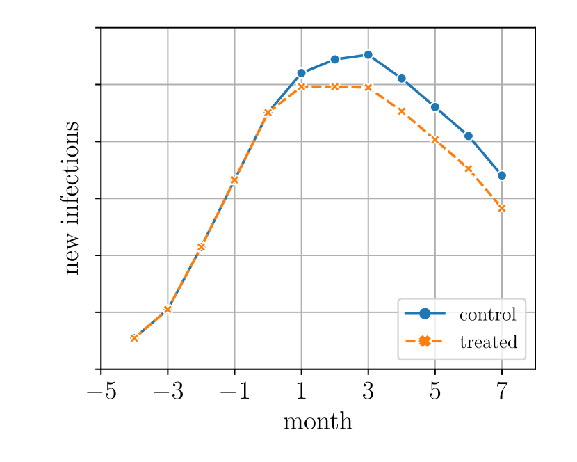
(a) Example 1

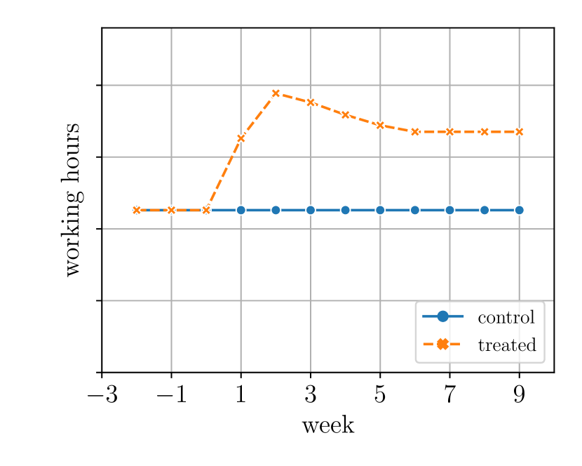
(b) Example 2

Figure 1: Illustrative examples of cumulative effects. These figures show the cumulative effects $\tau_{0}+\cdots+\tau_{j}$ as a function of the number of treated periods $j$. Figure 1(a) illustrates a scenario where the effect of a new public health intervention on new infections accumulates over time ($\tau_{0},\tau_{1},\tau_{2}<0$). Figure 1(b) illustrates a scenario where the effect of a new app feature on drivers’ working hours attenuates over time ($\tau_{0},\tau_{1}>0$ and $\tau_{2},\tau_{3},\tau_{4},\tau_{5}<0$).

Next we introduce the potential outcome model.

[Potential Outcome Model] The potential outcomes for unit $i$ at time $t$ can be written as

$$Y_{it}(z_{i,t-\ell},\cdots,z_{i,t-1},z_{it})$$

for a nonnegative integer $\ell$, where $\ell$ is known.

Assumption 1 requires that a unit’s treatment $z_{it}$ only affects this unit’s own outcomes (no cross-unit interference). It further requires that a unit’s outcomes are not affected by this unit’s future treatment assignments (no anticipation). For example, drivers do not increase their working hours in anticipation of the new app feature. No anticipation is also commonly imposed in the literature (Basse et al. 2023, Bojinov et al. 2023).

We allow the potential outcomes to depend on the treatment assignments up to $\ell$ periods in the past. We assume $\ell$ is known for the design and estimation purposes. Note that there exists a bias-variance tradeoff in the specification of $\ell$ in practice. When the specified $\ell$ is less than the true value, the estimator can be biased. When the specified $\ell$ is more than the true value, the estimator is unbiased, but can be inefficient. See Figure LABEL:fig:varying-ell in Section LABEL:ecsec:spec-ell for an example.

We define the average instantaneous effect $\tau_{0}$ and lagged effects $\tau_{1},\dots,\tau_{\ell}$ as

$$\tau_{j}\coloneqq\frac{1}{NT}\sum_{i,t}\frac{1}{2}\Big{[}Y_{it}(-1,\cdots,-1,\underbrace{+1}_{z_{i,t-j}},+1,\cdots,+1)-Y_{it}(-1,\cdots,-1,\underbrace{-1}_{z_{i,t-j}},+1,\cdots,+1)\Big{]}\,,$$

for all $j\in\{0\}\cup[\ell]$. Here $1/2$ is used for notation simplicity in the specification (1) below and remaining sections to account for the scaling of $z_{it}$ that takes value between $\{+1,-1\}$ as opposed to $\{+1,0\}$. Note that $\tau_{j}$ is the average, over individuals and time periods, of individual-time specific treatment effects that can be heterogeneous in both units and time periods.

Here $\tau_{0},\tau_{1},\cdots,\tau_{\ell}$ can take arbitrary values, and therefore allow for general dynamics of cumulative effects over time. To demonstrate this generality, we describe a few scenarios below.

• The average effect accumulates over time, for example when $\tau_{0},\ldots,\tau_{\ell}$ all have the same sign, as shown in Figure 1(a).

• The average effect attenuates over time, for example when $\tau_{0}$ and $\tau_{1}$ have a different sign than all of $\tau_{2},\ldots,\tau_{\ell}$, as shown in Figure 1(b).

• The average effect is constant over time, for example when $\ell=0$.

• The average cumulative effect is zero, for example when $\sum_{j=0}^{\ell}\tau_{j}=0$. After $\ell$ periods, a unit’s outcome is the same as the outcome of never being treated.

In this paper, we are interested in estimating $\bm{\tau}=(\tau_{0},\tau_{1},\cdots,\tau_{\ell})$. Below we study how to choose $Z=[z_{it}]_{(i,t)\in[N]\times[T]}$ to accurately estimate these parameters.

3 Non-Adaptive Experiments

In this section, we study the staggered rollout design of non-adaptive experiments. In Section 3.1, we present an approach for estimating $\tau_{0},\tau_{1},\cdots,\tau_{\ell}$. Next, in Section 3.2, we define the precision of the proposed estimators. We formulate an optimization problem, where for a given estimator, the solution yields the set of treatment times for each unit that maximizes the precision of the estimator. Finally, we present our solution to the optimization problem in Section 3.3.

3.1 Estimation of Instantaneous and Lagged Effects

The decision maker needs to consider two objectives when choosing an estimator for $\tau_{0},\tau_{1},\cdots,\tau_{\ell}$. First is the statistical properties of this estimator, such as the bias, variance, and mean-squared error (MSE). Second is the feasibility of optimizing units’ treatment times based on the properties of this estimator. For example, one can study the optimal treatment assignments based on MSE of a simple estimator such as the difference-in-means estimator, but this simple estimator can have a large variance and MSE. Alternatively, one can use a sophisticated estimator with a small MSE such as regularized matrix factorization estimator in Section LABEL:sec:algorithm, but the functional form of MSE may be very complex, which can lead to an intractable optimization problem in the design phase.

In this paper, we seek to balance these two objectives. We study the optimization of treatment assignments, for a particular estimator, namely the Generalized Least Squares (GLS) estimator, given a particular model for the data generating process. The GLS estimator for $\tau_{0},\tau_{1},\cdots,\tau_{\ell}$ is based on the following specification

$$Y_{it}=\alpha_{i}+\beta_{t}+\mathbf{X}_{i}^{\top}\bm{\theta}_{t}+\tau_{0}z_{it}+\tau_{1}z_{i,t-1}+\cdots+\tau_{\ell}z_{i,t-\ell}+\underbrace{\mathbf{u}_{i}^{\top}\mathbf{v}_{t}+\varepsilon_{it}}_{e_{it}}\,,$$ (1)

where $\alpha_{i}$ and $\beta_{t}$ are unobserved unit and time fixed effects, $\mathbf{X}_{i}\in\mathbb{R}^{d_{x}}$ are observed covariates of dimension $d_{x}$, $\bm{\theta}_{t}\in\mathbb{R}^{d_{x}}$ are their (non-random) unobserved time-varying coefficients $\bm{\theta}_{t}$, $\mathbf{u}_{i}\in\mathbb{R}^{d_{u}}$ are latent (non-random) covariates of dimension $d_{u}$, $\mathbf{v}_{t}\in\mathbb{R}^{d_{u}}$ are (random) latent factors, and $\{\varepsilon_{it}\}_{it\in[N]\times[T]}$ are unobserved residuals. We allow $d_{x}=0$, that is, (1) does not have observed covariates. We also allow $d_{u}=0$, that is, (1) does not have latent covariates.

The specification with two-way (i.e., unit and time) fixed effects and possibly with observed covariates has been widely used in observational studies to estimate treatment effects (Angrist and Pischke 2008). Observed covariates $\mathbf{X}_{i}$ in (1) are time-invariant and are not affected by the treatment. Examples of such covariates are an individual’s gender and race or attributes of a city. Using $\alpha_{i}$, $\beta_{t}$ and $\mathbf{X}_{i}$ controls for the heterogeneity in units and time periods, that can effectively reduce variance in treatment effect estimation. Note that (1) has the interactive latent factor structure $\mathbf{u}_{i}^{\top}\mathbf{v}_{t}$ that can capture the multiplicative unobserved effects, and is therefore more general than the specification with additive effects $\alpha_{i}$ and $\beta_{t}$ only. We assume $\mathbf{v}_{t}$ is random, but $\mathbf{u}_{i}$ is nonrandom for the design purpose. Such an assumption is also imposed in a different literature that estimates the latent factors on large panels (Bai and Ng 2002, Bai 2003).

GLS estimates $\tau_{0},\cdots,\tau_{\ell}$, $\alpha_{i}$, $\beta_{t}$ and $\bm{\theta}_{t}$ by minimizing the weighted sum of squared residuals $e_{it}$ in (1) (see Section 7.1 for more details). GLS has two nice properties when the optimal weights are chosen, following the Gauss-Markov Theorem (see Lemma 7.4 in Section 7.1) under the strict exogeneity assumption in Assumption 3.1 below. First, GLS is the best linear unbiased estimator (BLUE) of $\tau_{0},\cdots,\tau_{\ell}$, meaning that this estimator has the smallest variance among all the linear unbiased estimators. Second, there is an explicit formula for the variance and precision of GLS in terms of $z_{it}$, which makes the treatment design problem tractable.

[Error Structure] $\mathbf{v}_{t}\in\mathbb{R}^{d_{u}}$ is i.i.d. in $t$ with $\mathbb{E}[\mathbf{v}_{t}\mid\bm{\xi}_{it}]=\bm{0}$ and $\mathbb{E}[\mathbf{v}_{t}\mathbf{v}_{s}^{\top}\mid\bm{\xi}_{it},\bm{\xi}_{js}]=\bm{\Sigma}_{v}\cdot\bm{1}_{t=s}$ for all $i,j,t$ and $s$, where $\bm{\xi}_{it}=(\mathbf{X}_{i},z_{it},\cdots,z_{i-\ell,t})$. Moreover, $\varepsilon_{it}$ is i.i.d. in $i$ and $t$ with $\mathbb{E}[\varepsilon_{it}\mid\bm{\xi}_{it}]=0$ and $\mathbb{E}[\varepsilon_{it}\varepsilon_{js}\mid\bm{\xi}_{it},\bm{\xi}_{js}]=\sigma_{\varepsilon}^{2}\cdot\bm{1}_{i=j,t=s}$ for all $i,j,t$ and $s$. In addition, $\varepsilon_{it}$ is independent of $\mathbf{v}_{s}$ for all $i,t$ and $s$.

Remark 3.1 (Machine learning heuristics for $\bm{\tau}$)

Instead of focusing on the least squares estimator, one can look at other estimators, for example, machine learning estimators. We provide one such estimator in Section LABEL:sec:algorithm for $\bm{\tau}$ that does not rely on Assumption 3.1 about $\mathbf{v}_{t}$. This type of machine learning-based estimators are typically biased in the estimation of $\bm{\tau}$, but could have a smaller variance than the unbiased estimators. The optimization of $Z$ based on these estimators is generally not tractable, and therefore we do not emphasize them in this paper.

Remark 3.2 (Implication of Assumption 3.1)

$\mathbb{E}[\mathbf{v}_{t}]=0$ holds without loss of generality, as we can always project their mean to $\alpha_{i}$. Under Assumption 3.1, $e_{it}$ satisfies

$$\mathbb{E}[e_{it}]=0,\qquad\mathbb{E}[e_{it}^{2}]=\mathbf{u}_{i}^{\top}\mathbf{\Sigma}_{v}\mathbf{u}_{i}+\sigma_{\varepsilon}^{2},\qquad\mathbb{E}[e_{it}e_{jt}]=\mathbf{u}_{i}^{\top}\mathbf{\Sigma}_{v}\mathbf{u}_{j},\qquad\mathbb{E}[e_{it}e_{js}]=0,\quad\text{ for }\,\,t\neq s,$$

implying that $e_{it}$ is correlated in the unit dimension, but it is uncorrelated in the time dimension.

Remark 3.3 (Feasiblity of GLS)

The weight matrix $\mathbf{W}$ in GLS is optimal when it is proportional to the inverse covariance matrix of $\bm{e}_{t}=[e_{it}]_{i\in[N]}$, i.e., $\big{(}\mathbf{U}\mathbf{\Sigma}_{v}\mathbf{U}^{\top}+\sigma_{\varepsilon}^{2}\mathbf{I}_{N}\big{)}^{-1}$ with $\mathbf{U}=[\mathbf{u}_{i}]_{i\in[N]}$. As the optimal weight matrix is unknown, in practice, we can use feasible GLS, where we first use OLS, estimate the optimal weight matrix, and then use GLS with the estimated weight matrix.

Remark 3.4 (Treatment Effect Estimation with Heterogeneity)

Specifications like (1) have been commonly used to estimate average treatment effects in empirical studies in many domains, such as economics (Card and Krueger 1994), operations (e.g., Cui et al. (2019), Cachon et al. (2019)), and healthcare (Abaluck et al. 2021). Such specifications do not restrict treatment effects to be homogeneous. In Remark 3.17 below, we discuss an alternative estimation approach when heterogeneous treatment effects are the objects of interest.

3.2 Optimization Problems for Treatment Decisions

In this section, we introduce the optimization problem to solve the optimal $Z$ based on the statistical properties of GLS. From a high level perspective, we are interested in precisely estimating $\bm{\tau}$. However, there are $\ell+1$ parameters in $\bm{\tau}$ and it is generally infeasible to find an $Z$ that simultaneously maximizes the precision of each of $\hat{\tau}_{0},\cdots,\hat{\tau}_{\ell}$ for $\ell\geq 1$. Instead, one needs to consider an objective function that summarizes the precision of each of $\hat{\tau}_{0},\cdots,\hat{\tau}_{\ell}$ into a scalar. There are two categories of objective functions that one may be interested in:

• Balancing the precision/variance of each of $\hat{\tau}_{0},\cdots,\hat{\tau}_{\ell}$

• Maximizing the precision of some linear combination of $\hat{\tau}_{0},\cdots,\hat{\tau}_{\ell}$

Examples of the objective functions related to the first category include (Atkinson et al. 2007)

• A-optimal design: minimizes the trace of $\mathrm{Var}(\hat{\bm{\tau}})$

• D-optimal design: minimizes the determinant of $\mathrm{Var}(\hat{\bm{\tau}})$

• T-optimal design: maximizes the trace of the inverse of $\mathrm{Var}(\hat{\bm{\tau}})$

An example of the objective functions related to the second category is

• Cumulative effect ($\sum_{j=0}^{\ell}\tau_{j}$): minimizes $\mathrm{Var}\big{(}\sum_{j=0}^{\ell}\hat{\tau}_{j}\big{)}$

When $\ell=0$, the four objective functions mentioned above are equivalent to one another. For general $\ell$, they are not equivalent, and the optimal treatment assignments for these four objectives can be different (but the difference can be small).

In this section, we focus on finding the optimal assignment $A=[A_{i}]_{i\in[N]}$, where $A_{i}\in[T]\cup\{\infty\}$ denotes the first time that unit $i$ adopts the treatment ($A_{i}=\infty$ means unit $i$ was never treated). Because the treatment is irreversible, there is a one-to-one mapping between $(z_{i1},z_{i2},\cdots,z_{iT})$ and $A_{i}$. Given the reduction to the $N$ adoption times we focus on analytically solving the T-optimal (or trace-optimal) design:

$${{\color[rgb]{0,0,0}\max_{A}\mathrm{tr}\big{(}\mathrm{Prec}(\hat{\bm{\tau}};A)\big{)},}}$$ (2)

where $\mathrm{Prec}(\hat{\bm{\tau}};A)$ is the precision matrix of $\bm{\tau}$ and is defined as the matrix inverse of the variance-covariance matrix of $\bm{\tau}$, $\mathrm{Var}(\hat{\bm{\tau}};A)$, when the assignment $A$ is used.

T-optimal design was first introduced by Atkinson and Fedorov (1975a) to discriminate between two competing regression models (e.g., to determine whether $\ell=\ell_{0}$ or $\ell=\ell_{1}$ is true, for distinct number of lags $\ell_{0}$ and $\ell_{1}$ in our setting). Since then, the T-optimal design has been studied by Atkinson and Fedorov (1975b), Uciński and Bogacka (2005), Wiens (2009), Dette et al. (2012, 2013, 2015) and others.

Solving the T-optimal design is generally challenging, even in some special cases (see Example 3.5). We provide the explicit optimality conditions for the integer program (2) in Section 3.3. Based on the optimality conditions, we provide an algorithm on choosing a design in Algorithm 2 in Section 7.7.1. Admittedly, the other three objectives mentioned above would be natural and of practical interest, especially the one that minimizes the variance of the estimated cumulative effect, $\mathrm{Var}\big{(}\sum_{j=0}^{\ell}\hat{\tau}_{j}\big{)}$. However, analytically solving the other three objectives is generally infeasible, as explained in Remark 3.6 below. Instead, one could numerically solve the other three objectives in practice. We visualize the numerical solutions for D-optimal design in Figure 9 in Section 7.3, which has a similar structure as our solutions to (2). We empirically show in Section 5 and Section LABEL:subsubsec:robustness-to-alternative-metrics that our solutions to (2) outperform the benchmark treatment designs measured by the objective of A-optimal design and $\mathrm{Var}\big{(}\sum_{j=0}^{\ell}\hat{\tau}_{j}\big{)}$.

Example 3.5

If $T=1$, $\ell=0$, and all the covariates are observed (i.e., $d_{u}=0$), (2) coincides with the offline optimization problem in Bhat et al. (2019), and is equivalent to the MAX-CUT problem and is NP-hard (Hayes 2002, Mertens 2006). In this paper, we focus on the case of low-dimensional covariates. Our solution from Algorithm 2 is provably close to the optimal integer solution to (2) for a large $N$.

Remark 3.6 (Challenges in alternative objectives)

Note that each entry in $\mathrm{Var}(\hat{\bm{\tau}})$ is a ratio of two polynomial functions of $z_{it}$, where the degrees of numerator and denominator are $2\ell$ and $2(\ell+1)$, respectively, for $\ell\geq 1$. The objective of A-optimal design and $\mathrm{Var}\big{(}\sum_{j=0}^{\ell}\hat{\tau}_{j}\big{)}$ are both sums of entries in $\mathrm{Var}(\hat{\bm{\tau}})$ (i.e., sums of ratios of two higher-order polynomials of $z_{it}$). The objective of D-optimal design is the inverse of a $2(\ell+1)$-th order polynomial function of $z_{it}$. The objective functions of both A-optimal and D-optimal design are non-convex. Therefore, using the first order condition only is generally not sufficient to solve the global optimal solution.

3.3 Optimal Solutions

We provide the optimality conditions for the T-optimal design. The optimality conditions disentangle the effect of different components in (1) (i.e., two-way fixed effects, observed and latent covariates) on the optimal treatment assignments. This problem is challenging in our setting with multiple units and periods for two reasons. First, different components can potentially affect the optimal design in both unit and time dimensions. Second, the effect of different components may be convoluted and interact with one another.

To build intuition, we start with the solution to a simple specification.

Example 3.7 (Two-way fixed effects and $\ell=0$)

Suppose $Y_{it}=\alpha_{i}+\beta_{t}+\tau_{0}z_{it}+\varepsilon_{it}$, and and Assumptions 2, 1, and 3.1 hold. Then the objective function in (2) equals to

$$\mathrm{Prec}(\hat{\tau}_{0};A)=\frac{N}{\sigma_{\varepsilon}^{2}}\left[-2\bm{b}_{T}^{\top}\bm{\omega}-\bm{\omega}^{\top}\mathbf{P}_{\bm{1}_{T}}\bm{\omega}\right],$$ (3)

which is a quadratic and concave function of $\bm{\omega}=[\omega_{t}]_{t\in[T]}$ with $\omega_{t}=N^{-1}\sum_{i=1}^{N}z_{it}$, $\mathbf{P}_{\bm{1}_{T}}=\mathbf{I}_{T}-\bm{1}_{T}\bm{1}_{T}^{\top}/T$, and $\mathbf{b}_{T}=[b_{t}]$ with $b_{t}=(T+1-2t)/T$. By solving the first-order condition, we can show that any treatment design satisfying ${\omega}^{\ast}_{t}=-b_{t}$ for all $t$ is optimal and maximizes the precision. In the optimal solution, the treated fraction is linear in time. This result is conceptually similar to those in Lawrie et al. (2015), Girling and Hemming (2016), Li et al. (2018) that show the optimal treated fraction is linear in time, under a similar specification, but with $\alpha_{i}$ to be random effects. More intuition for the linear treated fraction is provided in Section 3.3.1.

Next consider a more general specification with $\ell>0$, but without $\mathbf{X}_{i}$ or $\mathbf{u}_{i}$. We can show the objective function in (2) is still quadratic and concave in $\bm{\omega}$, but takes a more complicated form (see Lemma 7.9 in Section 7.8), leading to nonlinear optimal treated fraction in time. Specifically in Theorem 3.8 we show that in the optimal solution, the unit average of $z_{it}$ satisfies

$$\omega_{\ell,t}^{\ast}=\begin{cases}-1&t\leq\lfloor\ell/2\rfloor\\ a^{(\ell)}_{t-\lfloor\ell/2\rfloor}&\lfloor\ell/2\rfloor<t\leq\ell\\ -1+\big{(}2t-(\ell+1)\big{)}/(T-\ell)&\ell<t\leq T-\ell\\ -\omega^{\ast}_{\ell,T+1-t}&T-\ell<t\leq T-\lfloor\ell/2\rfloor\\ 1&T-\lfloor\ell/2\rfloor<t\\ \end{cases}$$ (4)

where $a^{(\ell)}$ is a vector of length $\ell-\lfloor\ell/2\rfloor$ defined in Section 7.2. $\omega_{\ell,t}^{\ast}$ has five stages and follows an $S$-shaped curve in time $t$: stage 1: all units are under control; stage 2: $\omega_{t}^{\ast}$ grows non-linearly in time (because of $a^{(\ell)}$); stage 3: $\omega_{t}^{\ast}$ grows linearly in time; stage 4: $\omega_{t}^{\ast}$ grows non-linearly in time again; stage 5, all units are under treatment. The optimal solution is symmetric with respect to the center (i.e., $\left((T+1)/2,0\right)$). Figure 2 demonstrates $\omega_{\ell,t}^{\ast}$ for various $\ell$ in a $T=12$ period problem. More examples of $\omega_{\ell,t}^{\ast}$ will be provided in Section 3.3.1.

Furthermore, suppose the specification contains at least one of the $\mathbf{X}_{i}$ or $\mathbf{u}_{i}$ components. A commonly used variance reduction approach in cross-sectional studies is to balance covariates, so that treated and control units are comparable when the two groups have similar covariates (e.g., Imbens and Rubin (2015)). Similar intuition carries over to the panel setting. We show in Theorem 3.8 below that the optimal design balances covariates groups, where groups are defined as the set of units with the same initial treatment time.

We state the first of our main theorems using the following solution concepts: Let $\mathbb{A}_{\ell}=\big{\{}A:N^{-1}\sum_{i=1}^{N}\bm{1}_{A_{i}\leq t}=(1+\omega_{\ell,t}^{\ast})/2,\,\forall t\big{\}}$ be the set of designs satisfying (4). When $d_{x}>0$, let $\mathbb{A}_{\mathbf{X}}=\big{\{}A:N^{-1}\sum_{i=1}^{N}\mathbf{X}_{i}\bm{1}_{A_{i}=t}=\bm{0}_{d_{x}},\,\forall t\in\{2,\cdots,T\}\big{\}}$ be the set of designs satisfying covariate balancing conditions (suppose rows in $\mathbf{X}=[\mathbf{X}_{i}]_{i\in[N]}$ are centered). When $d_{x}=0$, let $\mathbb{A}_{\mathbf{X}}=\mathbb{A}^{N}$ and no conditions need to be imposed related to $\mathbf{X}_{i}$. $\mathbb{A}_{\mathbf{U}}$ is defined similarly as $\mathbb{A}_{\mathbf{X}}$.

Theorem 3.8 (Optimality Conditions)

Suppose Assumptions 2, 1, and 3.1 hold, $\hat{\bm{\tau}}$ is estimated from the infeasible GLS with $\mathbf{W}\propto\big{(}\mathbf{U}\mathbf{\Sigma}_{v}\mathbf{U}^{\top}+\sigma_{\varepsilon}^{2}\mathbf{I}_{N}\big{)}^{-1}$, rows in $\mathbf{X}$ and $\mathbf{U}$ are centered $($i.e., $\sum_{i=1}^{N}\mathbf{X}_{i}=\bm{0}_{d_{x}}$ and $\sum_{i=1}^{N}\mathbf{u}_{i}=\bm{0}_{d_{u}}$$)$, $\mathbf{X}$ and $\mathbf{U}$ are orthogonal $($i.e., $\sum_{i=1}^{N}\mathbf{X}_{i}\mathbf{u}_{i}^{\top}=\mathbf{0}_{d_{x}\times d_{u}}$$)$, $\mathbf{\Sigma}_{v}=\sigma_{\varepsilon}^{2}\cdot\mathbf{I}_{d_{u}}$, and $T>(\ell^{3}+13\ell^{2}+7\ell+3)/(8\ell)$. $A$ is an optimal treatment design if $A\in\mathbb{A}_{\mathrm{opt}}$, where

$$\mathbb{A}_{\mathrm{opt}}=\mathbb{A}_{\ell}\cap\mathbb{A}_{\mathbf{X}}\cap\mathbb{A}_{\mathbf{U}}\,.$$ (5)

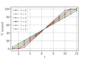
Figure 2: T-optimal design. Optimal treated fraction in the design of 12-period non-adaptive experiments with varying $\ell$.

Theorem 3.8 provides the optimality conditions for the T-optimal design when $\tau_{0},\cdots,\tau_{\ell}$ are estimated from GLS using specification (1). The presence of $\alpha_{i}$ and $\beta_{t}$ makes the optimal treated fraction grow gradually over time, and the growth rate is determined by $\ell$. We further illustrate how the optimal treated fractions depend on $\alpha_{i}$, $\beta_{t}$, and $\ell$ in Section 3.3.1. The presence of $\mathbf{X}_{i}$ and $\mathbf{u}_{i}$ imposes additional covariate balancing conditions, that can be satisfied if units in each stratum satisfy treated fraction conditions. Here strata are defined as groups of units with the same covariate value. When covariates are discrete-valued, Example 3.9 below provides a solution that satisfies the optimality conditions. For general cases, we provide guidance on choosing a design based on Theorem 3.8 in Section 3.3.2.

Example 3.9 (Discrete $\mathbf{X}_{i}$ and $\mathbf{u}_{i}$)

Suppose $(\mathbf{X}_{i},\mathbf{u}_{i})$ is discrete and can only take $G$ values for a finite $G>0$, denoted as $\{(x_{g},u_{g})\}_{g=1}^{G}$, each with positive probability. Then any $A$ in $\mathbb{A}^{\mathrm{disc}}_{\mathrm{opt}}$ defined below is in $\mathbb{A}_{\mathrm{opt}}$

$$\mathbb{A}^{\mathrm{disc}}_{\mathrm{opt}}=\bigg{\{}A:\frac{1}{|\mathcal{O}_{g}|}\sum_{i\in\mathcal{O}_{g}}\bm{1}_{A_{i}\leq t}=\frac{1+\omega_{\ell,t}^{\ast}}{2}\,\,\,\,\forall t,g\bigg{\}}\,,$$ (6)

where $\mathcal{O}_{g}=\{i:(\mathbf{X}_{i},\mathbf{u}_{i})=(x_{g},u_{g})\}$.

Remark 3.10 (Assumptions in Theorem 3.8)

The assumptions in Theorem 3.8 are non-restrictive for the following four reasons. First, the assumption that rows in $\mathbf{X}$ and $\mathbf{U}$ are demeaned can be satisfied by projecting the mean onto the unit fixed effects $\bm{\alpha}$. Second, the assumption that $\mathbf{X}$ and $\mathbf{U}$ are orthogonal can be satisfied by applying the Gram-Schmidt procedure (i.e., QR decomposition) to $\begin{bmatrix}\mathbf{X}&\mathbf{U}\end{bmatrix}$ (which is possible as $\bm{\theta}$ is unknown and unrestricted). Third, $\mathbf{\Sigma}_{v}=\sigma_{\varepsilon}^{2}\cdot\mathbf{I}_{d_{u}}$ is essentially an identification assumption, so that we can uniquely identify $\mathbf{u}_{i}$ and $\mathbf{v}_{t}$. Fourth, the fundamental structure of our problem does not change with these assumptions because $\mathrm{Prec}(\hat{\bm{\tau}})$ is a quadratic function of $z_{it}$ regardless of whether these assumptions are imposed or not.

Remark 3.11 (Assumption on $T$)

The assumption $T>(\ell^{3}+13\ell^{2}+7\ell+3)/(8\ell)$ is a sufficient condition to show $\omega_{\ell,t}^{\ast}$ is monotonic, but is not a necessary condition and can potentially be relaxed, based on the numerical solution of treated fractions when this assumption is violated.

Remark 3.12 (Magnitude of treatment effects)

Note that $\mathbb{A}_{\mathrm{opt}}$ and $\mathbb{A}^{\mathrm{disc}}_{\mathrm{opt}}$ do not depend on the value of $\bm{\tau}$. This is because the estimation error $\hat{\bm{\tau}}-\bm{\tau}$ from GLS does not depend on the value of $\bm{\tau}$ under the specification (1). Therefore, $\mathrm{tr}\big{(}\mathrm{Prec}(\hat{\bm{\tau}})\big{)}$ does not depend on the value of $\bm{\tau}$. See (3) for an example.

3.3.1 Optimal Treated Fractions

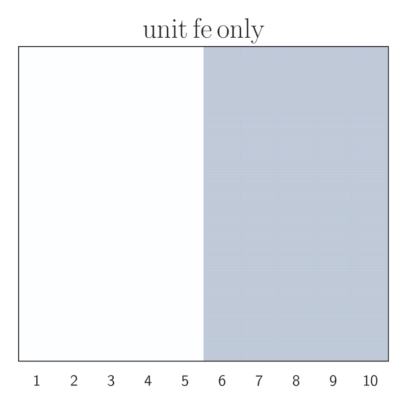
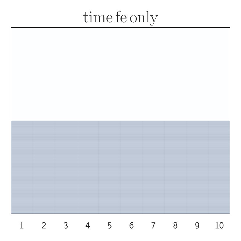
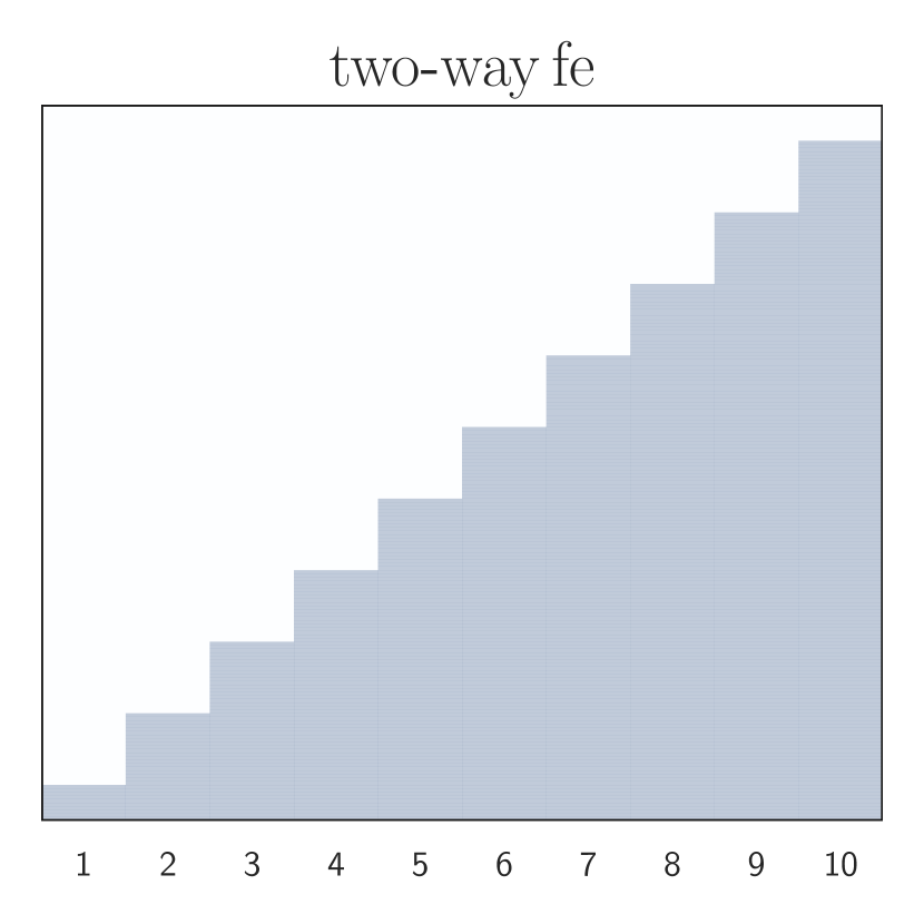
Figure 3: Optimal treatment designs under various specifications. Examples of T-optimal designs of $10$-period experiments with $\ell=0$. Darker color denotes treatment, and lighter color denotes control. “fe” stands for “fixed effects” and “covar” stands for “covariates”

To provide more intuition on the optimal treated fractions, we start with the specification with $\ell=0$, and with either $\alpha_{i}$ or $\beta_{t}$, but not both.

Example 3.13 (Time Fixed Effects Only and $\ell=0$)

Suppose $Y_{it}=\beta_{t}+\tau_{0}z_{it}+\varepsilon_{it}$ and Assumptions 2, 1, and 3.1 hold. In this case, $\mathrm{Prec}(\hat{\tau}_{0})={N}/{\sigma_{\varepsilon}^{2}}\cdot\big{[}T-\sum_{t=1}^{T}\omega_{t}^{2}\big{]}$. Any treatment design is optimal if it satisfies $\omega^{\ast}_{t}=0$ for all $t$ and $z_{it}\leq z_{i,t+1}$ for all $i$ and $t$, that is, assigns treatment to 50% units, while the others functioning as the control, for all time periods.

Example 3.14 (Unit Fixed Effects Only and $\ell=0$)

Suppose $Y_{it}=\alpha_{i}+\tau_{0}z_{it}+\varepsilon_{it}$ and Assumptions 2, 1, and 3.1 hold. In this case, $\mathrm{Prec}(\hat{\tau}_{0})={T}/{\sigma_{\varepsilon}^{2}}\cdot\big{[}N-\sum_{i=1}^{N}\zeta_{i}^{2}\big{]}$, where $\zeta_{i}=T^{-1}\sum_{t=1}^{T}z_{it}$. Any treatment design is optimal if it satisfies $\omega^{\ast}_{t}=-1$ for all $t<(T+1)/2$ and $\omega^{\ast}_{t}=1$ for all $t>(T+1)/2$, that is, allocates treatment to all units at halftime.

If the specification has both $\alpha_{i}$ and $\beta_{t}$, as in Example 3.7, the optimal treated fractions are intuitively in between those in Examples 3.13 and 3.14. See Figure 3 for the visualization of optimal treated fractions under various specifications.

The same intuition carries over to $\ell>0$ and the precision matrix $\mathrm{Prec}(\hat{\bm{\tau}})$ is quadratic and concave in $\omega_{t}$. The two examples below provide the analytic expression of $\omega^{\ast}_{\ell,t}$ for $\ell=1$ and $2$. We provide the expression of $\omega_{\ell,t}^{\ast}$ for $\ell=3$ in Example 7.5 of Section 7.2.

Example 3.15 ($\ell=1$)

In Theorem 3.8, $\omega^{\ast}_{\ell,t}$ equals $-1+{2(t-1)}/{(T-1)}$ for all $t$.

Example 3.16 ($\ell=2$)

In Theorem 3.8, $\omega^{\ast}_{\ell,t}$ is determined by, $\omega_{\ell,1}^{\ast}=-1$, $\omega_{\ell,2}^{\ast}=-1+{2}/{(2T-5)}$, $\omega_{\ell,t}^{\ast}=-1+{(2t-3)}/{(T-2)}$ for $t=3,\cdots,T-2$, $\omega_{\ell,T-1}^{\ast}=1-{2}/{(2T-5)}$, and $\omega_{{\ell,T}}^{\ast}=1$.

Intuition for the $S$-shaped curve of $\omega_{\ell,t}^{\ast}$.

The objective function in (2) is a sum of $\ell+1$ quadratic functions, one function for each $\mathrm{Prec}(\hat{\tau}_{j})$ with $j\in\{0,1,\cdots,\ell\}$. Let $\omega_{\ell,t}^{\ast}(j)$ be the unit average of $z_{it}$ in the solution that maximizes $\mathrm{Prec}(\hat{\tau}_{j})$ at time $t$, when the duration of lagged effects is $\ell$. This means $\omega^{\ast}_{\ell,t}$, defined in (4), can be written as a convex combination of $\omega_{\ell,t}^{\ast}(j)$ for all $j$ and $t$. Intuitively, since each $\omega_{\ell,t}^{\ast}(j)$ is chosen to maximize the precision of a single parameter $\hat{\tau}_{j}$, it should grow linearly in $t$, like the $\ell=0$ case, except during the first $\ell$ or the last $\ell$ periods that it is truncated to $0$ or $1$ respectively (see Figure 4). Equipped with this observation, it is easy to see that $\omega^{\ast}_{\ell,t}$ grows linearly in $t$ in the middle (the third stage) where all $\omega^{\ast}_{\ell,t}$ grow linearly. $\omega^{\ast}_{\ell,t}$ is constant in stage one and five, where all $\omega^{\ast}_{\ell,t}$ are constant. Moreover, $\omega^{\ast}_{\ell,t}$ has a non-linear growth in stage two and four, because some of $\omega_{\ell,t}^{\ast}(j)$ are truncated to $0$ or $1$.

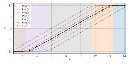
Figure 4: Illustration of the $S$-shaped curve for the $16$-period optimal design with $\ell=5$. For estimating $\tau_{j}$ only, the dashed lines denote the optimal $\omega_{t}$ that maximizes $\mathrm{Prec}(\hat{\tau}_{j})$ for $j\in\{0,1,\cdots,5\}$. For estimating $\tau_{0},\cdots,\tau_{5}$ simultaneously, the solid line denotes the optimal $\omega_{t}$ that maximizes $\mathrm{Prec}(\hat{\bm{\tau}})$, which is a convex combination of the dashed lines. The shaded regions from left to right denote the first to fifth stages in the solution $\omega^{\ast}_{\ell,t}$.

3.3.2 Choosing A Treatment Design

Based on the optimality conditions in Theorem 3.8, we provide Algorithm 2 in Section 7.6 to choose a treatment design. In this subsection, we outline some general guidance on choosing a treatment design. When the specification does not have covariates ($d_{x}=d_{u}=0$) and $\mathbb{A}_{\ell}$ is not empty, we can randomly choose one from $\mathbb{A}_{\ell}$ with equal probability. When the specification has observed, discrete-valued covariates ($d_{x}\neq 0$) and $\mathbb{A}^{\mathrm{disc}}_{\mathrm{opt}}$ is not empty, we can randomly choose one from $\mathbb{A}^{\mathrm{disc}}_{\ell}$ with equal probability. The random sampling can ensure that the treatment design balances the relevant covariates for the outcomes that are omitted in the specification (1) and design of experiments (Hayes and Moulton 2017).

Note that $\mathbb{A}^{\mathrm{disc}}_{\mathrm{opt}}$ can be empty, if $|\mathcal{O}_{g}|(1+\omega_{\ell,t}^{\ast})/(2T)$ is not an integer for each stratum (similarly for $\mathbb{A}_{\ell}$). For this case, Algorithm 2 rounds $|\mathcal{O}_{g}|(1+\omega_{\ell,t}^{\ast})/(2T)$ to the nearest integer to obtain a feasible design. As shown in Proposition 7.8 in Section 7.5, the value of $\mathrm{tr}\big{(}\mathrm{Prec}(\hat{\bm{\tau}})\big{)}$ evaluated at this feasible solution is within a factor of $1+O\left({1}/{N^{2}}\right)$ of the optimal value of $\mathrm{tr}\big{(}\mathrm{Prec}(\hat{\bm{\tau}})\big{)}$.

If observed covariates are continuous, then we can partition units into a small number of strata based on the observed covariate values, and then randomly choose a design that satisfies the treated fraction conditions for each stratum (possibly with rounding). Prior work has suggested keeping the number of strata small to avoid over-stratification (Kernan et al. 1999), because over-stratification may lower the precision of the estimated treatment effects (De Stavola and Cox 2008).

If there are latent covariates, we suggest using the historical control data for the same set of units for the design of experiments. We can improve precision by using historical data to estimate $\mathbf{u}_{i}$, partitioning units into strata (e.g., by spectral clustering), and choosing a treatment design based on the estimated $\mathbf{u}_{i}$. See Section 7.7 for more details.

Remark 3.17 (Conditional Average Treatment Effect (CATE))

Suppose we are interested in using observable sources of heterogeneity $\mathbf{X}_{i}$ to assess the heterogeneity in treatment effects (Robinson (1988), Wager and Athey (2018) among others). In this case, we may be interested in conditional average instantaneous and lagged effects, denoted by $\tau_{j}(\mathbf{X}_{i})$. If $\mathbf{X}_{i}$ is discrete, the designs satisfying (6) can maximize the precision of $\hat{\tau}_{j}(\mathbf{X}_{i})$ for all $j$ and $\mathbf{X}_{i}$, following that the optimality conditions for $\omega_{\ell,t}^{\ast}$ are satisfied within each stratum.

Remark 3.18 (Discussion on Adaptive Design)

The treatment assignments studied in this section are chosen and fixed before the experiment starts. For non-adaptive experiments, we do not pursue adaptive designs, where treatment assignments for subsequent periods can vary during the experiment, for the following reason. From Theorem 3.8, the information that matters for the treatment assignments but is unknown before the experiment starts is $\mathbf{u}_{i}$. However, the estimation of $\mathbf{u}_{i}$ at the beginning of the experiment can be quite noisy, and we do not expect noisy estimates of $\mathbf{u}_{i}$ can substantially help the design. See Section 7.7.2 for further elaboration on this.

4 Adaptive Experiments

Consider an experiment that is allowed to run $T_{\max}$ periods. The experimenter seeks to achieve a certain precision objective by the end of the experiment. After observing some data during the experiment, the experimenter may find that achieving this objective does not need $T_{\max}$ periods’ of experimental data. In this case, the experimenter may want to terminate the experiment early in order to reduce the cost of the experiment.

In this section, we study the design and analysis of adaptive experiments, where $N$ is fixed, but the experiment duration can vary due to the early termination. Let $\tilde{T}\in[T_{\max}]$ be the duration of the adaptive experiment, which is a random variable and unknown before the adaptive experiment starts. At any time period $t$, the experimenter collects data and decides whether to terminate the experiment. If so, the experiment stops, and the realization of $\tilde{T}$ is $t$; otherwise, the experimenter makes treatment decisions for time $t+1$. For ease of understanding, we present our algorithm and results based on the following simple specification of the observed outcome of unit $i$ at time $s$

$$Y_{is}=\alpha_{i}+\beta_{s}+\tau z_{is}+\varepsilon_{is},\qquad\forall~{}i\in[N],~{}s\in[\tilde{T}].$$ (7)

For simplicity, we denote instantaneous effect as $\tau$ instead of $\tau_{0}$ in this section. Later, we discuss how our algorithm and results can be generalized to the specification with $\ell>0$ and with $\mathbf{X}_{i}$ and $\mathbf{u}_{i}$.

Motivated by the objective of maximizing precision in (2), we consider the following criterion to terminate the experiment if the precision exceeds a target threshold $c$ at time $t$

$${{\color[rgb]{0,0,0}\mathrm{Prec}(\hat{\tau};\bm{\omega})=\frac{Nt}{\sigma_{\varepsilon}^{2}}\cdot\underbrace{(-2\bm{b}_{t}^{\top}\bm{\omega}_{1:t}-\bm{\omega}_{1:t}^{\top}\mathbf{P}_{\bm{1}_{t}}\bm{\omega}_{1:t})/t}_{g_{\tau}(\bm{\omega},t)}\geq c\,,}}$$ (8)

where the expression of $\mathrm{Prec}(\hat{\tau};\bm{\omega})$ follows from Example 3.7 in the case of $\hat{\tau}$ estimated from a panel with $N$ units and $t$ periods. In this section, we parametrize the precision by $\bm{\omega}$ and we optimize over $\bm{\omega}$, as the precision only depends on $\bm{\omega}$ but not whom to treat under specification (7). This precision-based rule is equivalent to the variance-based rule to terminate the experiment when $\mathrm{Var}(\hat{\tau})\leq 1/c$. This type of termination rules has been used by others in different settings, such as in simulations and in sequential testing on sequentially arrived units without time effects (Chow and Robbins (1965), Glynn and Whitt (1992a), Singham and Schruben (2012) among others).

There are three key technical challenges in designing and analyzing the experiments that can be terminated early. The first challenge concerns adaptively choosing the fraction of treated units per period. Recall from Example 3.7, that $\omega_{s}^{\ast}=(2s-1-\tilde{T})/\tilde{T}$. But, since $\tilde{T}$ is unknown before the experiment starts, or even during the experiment, choosing the optimal fraction of treated units is non-trivial. To address this challenge, we aim to adaptively improve the treatment decisions as we gather more information about $\tilde{T}$ during the experiment.

The second challenge concerns implementing the termination rule. As long as we can estimate the critical unknown parameter $\sigma_{\varepsilon}^{2}$ in (8), we can determine whether to stop the experiment. There are two main difficulties in this task. The first is to have a valid implementation of the termination rule on adaptively collected data. Here, valid implementation means that the precision indeed exceeds threshold $c$ when the experiment terminates. The second is to do it in a way that the next challenge (obtaining valid post-experiment inference of $\tau$) can be manageable. Early stopping complicates post-experiment inference because the same data is used to make the decision about stopping and to estimate treatment effects, leading to the well-known bias that can arise when adaptive tests determine whether to terminate experiments (Johari et al. (2017) among others).

The third challenge concerns efficient estimation and inference for $\tau$, post-experiment. Based on the adaptive nature of collected data and the implementation of experiment termination rule, we seek to choose a consistent and efficient estimator for $\tau$ that uses as many observations as possible.

We propose the Precision-Guided Adaptive Experiment (PGAE) algorithm in Section 4.2 to simultaneously tackle these three challenges. PGAE combines ideas from dynamic programming and sample splitting. In Section 4.3, we prove statistical consistency and asymptotic normality of $\hat{\tau}$ and $\widehat{\sigma^{2}}$, estimated by PGAE, paving the way for valid statistical inference for $\tau$.

4.1 Estimators

To start, we first review two existing estimators and then propose a new estimator. All three estimators are extensively used in PGAE. Suppose these estimators use the data of units in a set $\mathcal{S}$ over $t$ periods collected so far, where $t$ is small, but set size $|\mathcal{S}|$ can be large. In this subsection, we sub-index the estimators by $\mathcal{S}$ and $t$ to refer to the data used in the estimators.

The first is the within estimator for $\tau$ (Wallace and Hussain 1969). The within estimator of $\tau$, denoted by $\hat{\tau}_{\mathcal{S},t}$, regresses $\dot{Y}_{is}$ on $\dot{z}_{is}$ based on the specification $\dot{Y}_{is}=\tau\dot{z}_{is}+\dot{\varepsilon}_{is}$, where for any variables $\{x_{is}\}_{(i,s)\in\mathcal{S}\times[t]}$ (e.g., $Y_{is}$ and $z_{is}$), the notation $\dot{x}_{is}$ denotes the within transformed $x_{is}$ and is defined as

$$\dot{x}_{is}=x_{is}-\bar{x}_{i\cdot}-\bar{x}_{\cdot s}+\bar{x}\,,$$ (9)

in which $\bar{x}_{i\cdot}$, $\bar{x}_{\cdot s}$, and $\bar{x}$ are averages of $x_{is}$’s over time periods, units, and both of them, respectively. The within estimator is an efficient estimation approach that does not need to estimate $\alpha_{i}$ and $\beta_{s}$, but produces the same estimate of $\tau$ as OLS based on (7) that estimates $\alpha_{i}$ and $\beta_{s}$. As shown in Lemma 4.1, $\hat{\tau}_{\mathcal{S},t}$ is consistent and asymptotically normal for any finite $t$, when the set size $|\mathcal{S}|$ is large.

The second is the plug-in estimator for $\sigma^{2}_{\varepsilon}$, which is used in experiment termination and post-experiment inference, and takes the form of

$$\widehat{\sigma^{2}}_{\mathcal{S},t}=\frac{1}{|\mathcal{S}|\cdot(t-1)}\sum_{i\in\mathcal{S}}\sum_{s=1}^{t}\big{(}\dot{y}_{is}-\hat{\tau}_{\mathcal{S},t}\cdot\dot{z}_{is}\big{)}^{2}.$$ (10)

The factor $1/(t-1)$ is for finite $t$ correction. As shown in Lemma 4.1, $\widehat{\sigma^{2}}_{\mathcal{S},t}$ is consistent and asymptotically normal for any finite $t$.

The third is a new estimator for the variance of $\varepsilon_{is}^{2}$, that is, $\xi^{2}_{\varepsilon}\coloneqq\mathbb{E}[(\varepsilon^{2}_{is}-\sigma^{2}_{\varepsilon})^{2}]$, which is used to quantify the uncertainty in our estimator for $\sigma^{2}_{\varepsilon}$, and takes the form of

$$\widehat{\xi^{2}}_{\mathcal{S},t}= \underbrace{\frac{t^{2}}{(t-1)^{2}}}_{\begin{subarray}{c}\text{correction}\\ \text{multiplier}\end{subarray}}\cdot\underbrace{\frac{1}{|\mathcal{S}|\cdot t}\sum_{i\in\mathcal{S}}\left(\sum_{s=1}^{t}\left[(\dot{y}_{is}-\hat{\tau}_{\mathcal{S},t}\cdot\dot{z}_{is})^{2}-\widehat{\sigma^{2}}_{\mathcal{S},t}\right]\right)^{2}}_{\text{plug-in estimator of }\xi^{2}_{\varepsilon}}-\underbrace{\frac{3t-2}{(t-1)^{2}}\cdot(\widehat{\sigma^{2}}_{\mathcal{S},t})^{2}}_{\text{correction term}}\,.$$ (11)

In this estimator, both the correction multiplier and correction term are used to de-bias the plug-in estimator when $t$ is finite. The plug-in estimator is biased, because $(\dot{y}_{is}-\hat{\tau}_{\mathcal{S},t}\cdot\dot{z}_{is})^{2}$ is not an unbiased estimator of $\sigma^{2}_{is}$ for each $i$ and $s$, and the bias is squared in the estimation of $\xi_{\varepsilon}^{2}$, which cannot be averaged out over $i$. Figure LABEL:fig:test-asymptotics in Section LABEL:subsec:finite-sample-lemma visualizes the bias of the plug-in estimator and shows that $\widehat{\xi^{2}}_{\mathcal{S},t}$ can correct for the bias in finite samples. Lemma 4.1 shows that $\widehat{\xi^{2}}_{\mathcal{S},t}$ is consistent for any finite $t$.

4.2 Precision-Guided Adaptive Experiment (PGAE) via Dynamic Programming

PGAE simultaneously addresses the three challenges introduced at the beginning of Section 4, which is feasible through a careful partitioning of units into disjoint subsets, with each set functioning for a different purpose. Specifically, we partition units into three mutually disjoint sets $\mathcal{S}_{\mathrm{ntu}}$, $\mathcal{S}_{\mathrm{atu},1}$ and $\mathcal{S}_{\mathrm{atu},2}$ that represent a set of non-adaptive treatment units (NTU) and two sets of adaptive treatment units (ATU), respectively. See Figure 5 for an illustration. Let $p_{\mathrm{ntu}}=|\mathcal{S}_{\mathrm{ntu}}|/N$, $p_{\mathrm{atu},1}=|\mathcal{S}_{\mathrm{atu},1}|/N$, and $p_{\mathrm{atu},2}=|\mathcal{S}_{\mathrm{atu},2}|/N$ be the fractions of units in these three sets. Clearly, $p_{\mathrm{ntu}}+p_{\mathrm{atu},1}+p_{\mathrm{atu},2}=1$. The sets are selected such that $p_{\mathrm{ntu}}$ is small and $p_{\mathrm{atu},1}=p_{\mathrm{atu},2}$.

Before the experiment starts, we initialize the treatment designs of $\mathcal{S}_{\mathrm{ntu}}$, $\mathcal{S}_{\mathrm{atu},1}$ and $\mathcal{S}_{\mathrm{atu},2}$ by the optimal design of a $T_{\max}$-period non-adaptive experiment, which is the solution without early stopping. Then the average of $z_{is}$ over $i$ in each set satisfies $\omega_{\mathrm{bm},s}=(2s-1-T_{\max})/{T_{\max}}$ for all $s\in[T_{\max}]$ (with rounding if necessary), per Example 3.7. The initial design also serves as the “benchmark” design for the adaptive experiment. The treatment design of NTU does not change during the experiment, stays equal to $\bm{\omega}_{\mathrm{bm}}$, and observed data from NTU is used to update the treatment assignments of ATU for subsequent periods, specifically, to improve upon $\bm{\omega}_{\mathrm{bm}}$. One of the two ATU sets ($\mathcal{S}_{\mathrm{atu},1}$) is used to estimate $\sigma_{\varepsilon}^{2}$, and decide whether to terminate the experiment. The other ATU set ($\mathcal{S}_{\mathrm{atu},2}$) provides another estimate of $\sigma_{\varepsilon}^{2}$ for post-experiment inference. As we will see in Section 4.3, partitioning units into three sets is crucial for decoupling possible correlations due to data reuse and hence obtaining valid statistical inference.

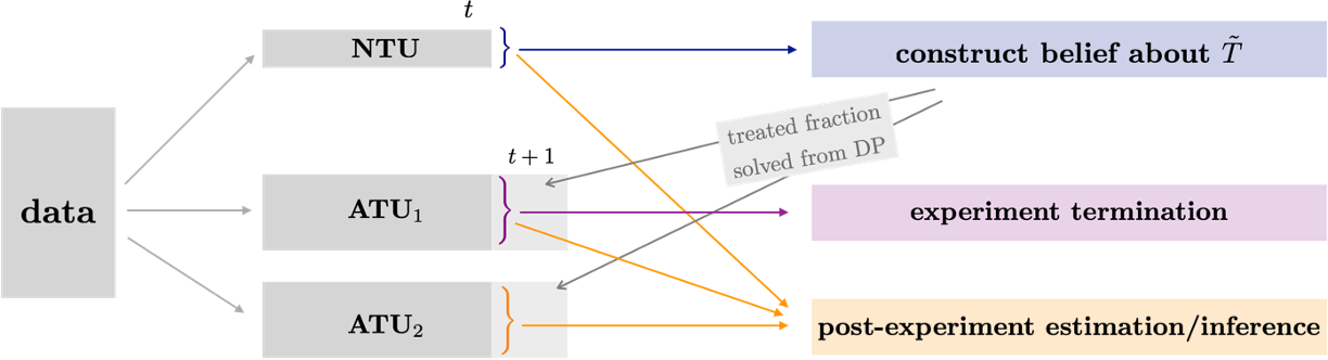
Figure 5: Illustration of PGAE.

Next, we illustrate how PGAE addresses each of the three challenges.

1. Choosing a treatment design.

In order to update treatment decisions for ATU, we need to construct a belief about experiment stopping time $\tilde{T}$, using NTU. If we would have known $\sigma_{\varepsilon}^{2}$, then we would exactly know the minimum stopping time $\tilde{T}$ such that the precision (using $\bm{\omega}_{\mathrm{bm}}$) is bigger than $c$ in (8). However, $\sigma_{\varepsilon}^{2}$ is unknown in practice, but it is possible to construct the belief distribution of $\sigma_{\varepsilon}^{2}$, which will be explained in detail below. Then we can draw samples of $\sigma^{2}$ from the belief distribution of $\sigma_{\varepsilon}^{2}$. For each sampled $\sigma^{2}$, we plug it into the precision expression and find the minimum duration that satisfies the stopping rule (8). The minimum duration may vary with the sampled $\sigma^{2}$. By repeatedly sampling $\sigma^{2}$ and finding the minimum duration, we can obtain an empirical distribution of $\tilde{T}$, denoted as $P_{t}(\tilde{T})$. See the pseudocode of the helper function estimate_belief() of PGAE in Section LABEL:subsec:pseudo-code for more details.

Here is our approach to constructing a belief distribution of $\sigma_{\varepsilon}^{2}$. We first estimate $\sigma_{\varepsilon}^{2}$ from formula (10) using data of NTU for $t$ periods. Let $\widehat{\sigma^{2}}_{\mathrm{ntu},t}$ be the estimator. Next, we quantify the uncertainty in $\widehat{\sigma^{2}}_{\mathrm{ntu},t}$. From Lemma 4.1 below, $\widehat{\sigma^{2}}_{\mathrm{ntu},t}$ is consistent and asymptotically normal with

$$\sqrt{|\mathcal{S}_{\mathrm{ntu}}|\cdot t}\cdot\frac{\widehat{\sigma^{2}}_{\mathrm{ntu},t}-\sigma_{\varepsilon}^{2}}{\hat{\xi}_{\mathrm{ntu},t}^{\dagger}}\xrightarrow{d}\mathcal{N}(0,1)\,,$$ (12)

where $\hat{\xi}_{\mathrm{ntu},t}^{\dagger}=\big{[}\widehat{\xi^{2}}_{\mathrm{ntu},t}+(\widehat{\sigma^{2}}_{\mathrm{ntu},t})^{2}/(t-1)\big{]}^{1/2}$ and $\widehat{\xi^{2}}_{\mathrm{ntu},t}$ is estimated from (11) using data of NTU. Let the left-hand side of (12) be $w$. We have $\sigma_{\varepsilon}^{2}=\widehat{\sigma^{2}}_{\mathrm{ntu},t}-w\cdot{\hat{\xi}^{\dagger}_{\mathrm{ntu},t}}/{\sqrt{|\mathcal{S}_{\mathrm{ntu}}|\cdot t}}$, and we repeatedly use this formula with samples of $w$ from $\mathcal{N}(0,1)$ to obtain a belief distribution of $\sigma_{\varepsilon}^{2}$.

We use a dynamic program to solve the treatment decisions for ATU. In this dynamic program, the state variable is the treated fractions up to time $t$, i.e., $\bm{\omega}_{\mathrm{atu},1:t}$, and the decision variable is the treated fraction for the next period $\omega_{t+1}$. The payoff in intermediate time periods is zero, and conditional on the realization of $\tilde{T}$, the terminal cost is $-\tilde{T}\cdot g_{\tau}\left((\bm{\omega}_{\mathrm{atu},1:t},\bm{\omega}_{(t+1):\tilde{T}}),\tilde{T}\right)$, which is equivalent to our objective of maximizing precision. Here, in the dynamic program, we aim to solve $\omega_{t+1}$ that minimizes the expected terminal cost. The expectation is taken with respect to the random experiment duration $\tilde{T}$, and we use the empirical distribution $P_{t}(\tilde{T})$ learned at time $t$ when taking the expectation. Specifically, we solve $\omega_{t}$ by minimizing

$$\mathbb{E}_{\tilde{T}\sim P_{t}(\tilde{T})}\left[-\tilde{T}\cdot g_{\tau}\left((\bm{\omega}_{\mathrm{atu},1:t},\bm{\omega}_{(t+1):\tilde{T}}),\tilde{T}\right)\right]\,,$$

subject to the constraint $\omega_{\mathrm{atu},t}\leq\omega_{t+1}\leq\omega_{t+2}\leq\cdots\leq\omega_{T_{\max}}\leq 1$. Section 9.1 provides more discussion on this dynamic program, and more details about the dynamic program can be found in the pseudocode of the helper function update_treatment_design() of PGAE in Section LABEL:subsec:pseudo-code.

2. Implementing the termination rule.

We use the data in $\mathcal{S}_{\mathrm{atu},1}$ to estimate $\sigma^{2}_{\varepsilon}$ via formula (10). Let the estimator at time $t$ be $\widehat{\sigma^{2}}_{\mathrm{atu},1,t}$. We then plug $\widehat{\sigma^{2}}_{\mathrm{atu},1,t}$ and $\bm{\omega}_{\mathrm{bm},1:t}$ into the termination rule (8) to estimate precision and decide whether to terminate the experiment. Note that using $\bm{\omega}_{\mathrm{bm},1:t}$ tends to under-estimate the precision (see Proposition 9.1 in Section 9.2), so that the experiment termination tends to be conservative. If our experiment terminates, we show in Proposition 9.2 in Section 9.2 that the true precision exceeds $c$ with a high probability.

3. Efficient estimation and valid inference for $\tau$.

In PGAE, we estimate $\tau$ using all the data of NTU and ATU over $\tilde{T}$ periods. Let the estimator be $\hat{\tau}_{\mathrm{all},\tilde{T}}$. We show in Theorem 4.3 below that $\hat{\tau}_{\mathrm{all},\tilde{T}}$ is efficient and achieves the optimal convergence rate. But we only use $\mathcal{S}_{\mathrm{atu},2}$ to estimate $\sigma^{2}_{\varepsilon}$ via formula (10). Let the estimator be $\widehat{\sigma^{2}}_{\mathrm{atu},2,\tilde{T}}$, which is consistent, and we use $\widehat{\sigma^{2}}_{\mathrm{atu},2,\tilde{T}}$ to estimate $\mathrm{Var}(\hat{\tau})$. Note that the consistency of $\sigma^{2}_{\varepsilon}$ is sufficient for constructing valid confidence intervals for $\tau$. Therefore the efficiency (determined by the sample size) in the estimation of $\sigma^{2}_{\varepsilon}$ is less important. The only tradeoff is that the endpoints of confidence intervals are estimated less precisely, with a larger second-order error term. This explains why we use only $\mathcal{S}_{\mathrm{atu},2}$ to estimate $\sigma^{2}_{\varepsilon}$.

In summary, PGAE takes advantage of all the data collected so far, and then jointly optimizes treatment assignments alongside the choice of whether to continue the experiment. The pseudocode for PGAE is shown in Algorithm 1, with the pseudocode for the helper functions collected in Section LABEL:subsec:pseudo-code.

Algorithm pgae($N,T_{\max},\bm{\omega}_{\mathrm{bm}},c,p_{\mathrm{ntu}},m,t_{0}$)

      1 $Z_{\mathrm{ntu}}$, $Z_{\mathrm{atu},1}$, $Z_{\mathrm{atu},2}\leftarrow$ partition_initialize($N,p_{\mathrm{ntu}},T_{\max}$)

      2 Run the experiment for $t_{0}$ time periods

      3 $\widehat{\sigma^{2}}_{\mathrm{atu},1,t},\widehat{\mathrm{Prec}}_{\mathrm{atu},1,t}\leftarrow$ estimate_var_prec($Z_{\mathrm{atu},1,1:t},Y_{\mathrm{atu},1,1:t},\bm{\omega}_{\mathrm{bm}},N,n_{\mathrm{atu}},t$)

      4 while $\widehat{\mathrm{Prec}}_{\mathrm{atu},1,t}<c$ and $t<T_{\max}$ do

            5 $P_{t}(\cdot)\leftarrow$ estimate_belief($Z_{\mathrm{ntu},1:t},Y_{\mathrm{ntu},1:t},N,\bm{\omega}_{\mathrm{bm}},T_{\max},t,m,c$)

            6 $Z_{\mathrm{atu},1,t+1},Z_{\mathrm{atu},2,t+1}\leftarrow$ update_treatment_design($Z_{\mathrm{atu},1,1:t},Z_{\mathrm{atu},2,1:t},\omega_{\mathrm{atu},1:t},T_{\max},t$)

            7 $t\leftarrow t+1$, and run the experiment for time period $t+1$

            8 $\widehat{\sigma^{2}}_{\mathrm{atu},1,t},\widehat{\mathrm{Prec}}_{\mathrm{atu},1,t}\leftarrow$ estimate_var_prec($Z_{\mathrm{atu},1,1:t},Y_{\mathrm{atu},1,1:t},\bm{\omega}_{\mathrm{bm}},N,n_{\mathrm{atu}},t$)

            

       end while

      9$\tilde{T}\leftarrow t$, and $\hat{\tau}_{\mathrm{all},\tilde{T}}\leftarrow$ within estimator of $\tau$ from both NTU and ATU

      10 $\widehat{\sigma^{2}}_{\mathrm{atu},2,\tilde{T}},\widehat{\mathrm{Prec}}_{\mathrm{atu},2,\tilde{T}}\leftarrow$ estimate_var_prec($Z_{\mathrm{atu},2,1:\tilde{T}},Y_{\mathrm{atu},2,1:\tilde{T}},\bm{\omega}_{\mathrm{bm}},N,n_{\mathrm{atu}},\tilde{T}$)

      11 return $\tilde{T}$, $\hat{\tau}_{\mathrm{all},\tilde{T}}$ and $\widehat{\sigma^{2}}_{\mathrm{atu},2,\tilde{T}}$

Algorithm 1 Precision-Guided Adaptive Experiment (PGAE)

4.3 Analysis of the Algorithm

In this subsection, we present the asymptotic results of the estimated $\tau$ and $\sigma^{2}_{\varepsilon}$ in PGAE. These results serve two purposes. The first is to justify our approach in Section 4.2 to construct a belief about $\sigma^{2}_{\varepsilon}$, and specifically to justify (12). The second is to show that the outputs of PGAE (i.e., $\hat{\tau}_{\mathrm{all},\tilde{T}}$ and $\widehat{\sigma^{2}}_{\mathrm{atu},2,\tilde{T}}$) can be used for valid statistical inference and hypothesis test of treatment effect.

To start, we characterize the asymptotic properties of $\hat{\tau}_{\mathrm{ntu},t}$, $\widehat{\sigma^{2}}_{\mathrm{ntu},t}$ and $\widehat{\xi^{2}}_{\mathrm{ntu},t}$, when they are estimated from non-adaptive experimental data, in Lemma 4.1. This lemma provides theoretical support for constructing the belief distribution of $\sigma_{\varepsilon}^{2}$, and serves as a crucial intermediate step in characterizing asymptotic distributions for the outputs of PGAE.

Lemma 4.1

Suppose Assumptions 2 and 1 hold. Under the specification (7), suppose $\varepsilon_{is}$ is i.i.d. for any $i$ and $s$ with $\mathbb{E}[\varepsilon_{is}]=0$, $\mathbb{E}[\varepsilon^{2}_{is}]=\sigma_{\varepsilon}^{2}$, $\mathbb{E}[\varepsilon^{3}_{is}]=0$, and $\mathbb{E}[(\varepsilon^{2}_{is}-\sigma^{2}_{\varepsilon})^{2}]=\xi^{2}_{\varepsilon}$. $\hat{\tau}_{\mathrm{ntu},t}$ and $\widehat{\sigma^{2}}_{\mathrm{ntu},t}$ are consistent. As $|\mathcal{S}_{\mathrm{ntu}}|\rightarrow\infty$, for any finite $t$, conditional on $Z_{\mathrm{ntu}}$, we have

$$\sqrt{|\mathcal{S}_{\mathrm{ntu}}|}\left(\begin{bmatrix}\hat{\tau}_{\mathrm{ntu},t}\\ \widehat{\sigma^{2}}_{\mathrm{ntu},t}\end{bmatrix}-\begin{bmatrix}\tau\\ \sigma^{2}_{\varepsilon}\end{bmatrix}\right)\stackrel{{\scriptstyle d}}{{\longrightarrow}}\mathcal{N}\left(\begin{bmatrix}0\\ 0\end{bmatrix},\begin{bmatrix}\sigma_{\varepsilon}^{2}/(t\cdot g_{\tau}(\bm{\omega}_{\mathrm{ntu},1:t},t))&0\\ 0&\xi_{\varepsilon,t}^{\dagger 2}/t\end{bmatrix}\right),$$

where $\xi_{\varepsilon,t}^{\dagger 2}=\xi^{2}_{\varepsilon}+2\big{(}\sigma_{\varepsilon}^{2}\big{)}^{2}/(t-1)$. Furthermore, $\sqrt{|\mathcal{S}_{\mathrm{ntu}}|}\big{(}\widehat{\xi^{2}}_{\mathrm{ntu},t}-\xi_{\varepsilon}^{2}\big{)}=O_{p}(1)$.

Since both $\widehat{\sigma^{2}}_{\mathrm{ntu},t}$ and $\widehat{\xi^{2}}_{\mathrm{ntu},t}$ are consistent, $\widehat{\xi^{\dagger 2}}_{\mathrm{ntu},t}=\widehat{\xi^{2}}_{\mathrm{ntu},t}+2\big{(}\widehat{\sigma^{2}}_{\mathrm{ntu},t}\big{)}^{2}/(t-1)$ is a consistent estimator of $\xi_{\varepsilon}^{\dagger 2}$. From Slutsky’s theorem, the asymptotic distribution in (12) holds.

Interestingly, $\hat{\tau}_{\mathrm{ntu},t}$ and $\widehat{\sigma^{2}}_{\mathrm{ntu},t}$ are asymptotically independent, even though we use $\hat{\tau}_{\mathrm{ntu},t}$ in the estimation of $\widehat{\sigma^{2}}_{\mathrm{ntu},t}$. The reason of asymptotic independence is as follows. The estimation error of $\hat{\tau}_{\mathrm{ntu},t}$ is a weighted average of $\varepsilon_{is}$ over $i$ and $s$. The leading term in the estimation error of $\widehat{\sigma^{2}}_{\mathrm{ntu},t}$ is the sum of a weighted average of $\varepsilon^{2}_{ju}-\sigma_{\varepsilon}^{2}$ over $j$ and $u$ and a weighted average of $\varepsilon_{ju}\varepsilon_{jv}$ over $j,u,v$ with $u\neq v$. Note that $\varepsilon_{is}$ is uncorrelated with both $\varepsilon^{2}_{ju}-\sigma_{\varepsilon}^{2}$ and $\varepsilon_{ju}\varepsilon_{jv}$ for all $i,j,s,u,v$, because $\varepsilon_{is}$ is i.i.d. in $i$ and $s$ and has zero first and third moments. Therefore, the leading terms in the estimation errors of $\hat{\tau}_{\mathrm{ntu},t}$ and $\widehat{\sigma^{2}}_{\mathrm{ntu},t}$ are uncorrelated. For the non-leading terms, they are at a small order of magnitude and do not contribute to the asymptotic covariance. As $\hat{\tau}_{\mathrm{ntu},t}$ and $\widehat{\sigma^{2}}_{\mathrm{ntu},t}$ are jointly asymptotically normal, the zero asymptotic correlation implies asymptotic independence. In Section LABEL:subsec:finite-sample-lemma, we demonstrate the finite sample properties of Lemma 4.1 and asymptotic independence between $\hat{\tau}_{\mathrm{ntu},t}$ and $\widehat{\sigma^{2}}_{\mathrm{ntu},t}$.

Remark 4.2

Lemma 4.1 holds for any finite $t$. In fact, when $t$ grows to infinity, the problem is simpler, because we can show $\mathrm{plim}_{t\rightarrow\infty}\xi^{\dagger 2}_{\varepsilon,t}=\xi^{2}_{\varepsilon}$, and the plug-in estimator of $\xi^{2}_{\varepsilon}$ mentioned in formula (11) is consistent. In this section, we focus on the challenging case with a finite $t$, because we want to apply Lemma 4.1 to the estimates on NTU early in the experiment (i.e., $t$ is small).

Next we show that $\hat{\tau}_{\mathrm{all},\tilde{T}}$ and $\widehat{\sigma^{2}}_{\mathrm{atu},2,\tilde{T}}$ from PGAE can be used for valid post-experiment statistical inference and hypothesis testing for $\tau$. To show this, there are two critical steps: (a) show the asymptotic distribution of $\hat{\tau}_{\mathrm{all},\tilde{T}}$; (b) show that the asymptotic variance of $\hat{\tau}_{\mathrm{all},\tilde{T}}$ can be consistently estimated using $\widehat{\sigma^{2}}_{\mathrm{atu},2,\tilde{T}}$.

Theorem 4.3

Suppose Assumptions 2 and 1 hold, $p_{\mathrm{ntu}}\in(0,1)$ is a fixed number as $N$ grows. Under the specification (7), suppose the assumptions about $\varepsilon_{is}$ in Lemma 4.1 hold and $\varepsilon_{is}$ is bounded with a symmetric distribution around $0$. $\hat{\tau}_{\mathrm{all},\tilde{T}}$ and $\widehat{\sigma^{2}}_{\mathrm{atu},2,\tilde{T}}$ are consistent. As $N\rightarrow\infty$,

$$\sqrt{N}\cdot\begin{bmatrix}\big{(}\tilde{T}g_{\tau}(\bm{\omega}_{\mathrm{all},1:\tilde{T}},\tilde{T})/\sigma_{\varepsilon}^{2}\big{)}^{1/2}\cdot\left(\hat{\tau}_{\mathrm{all},\tilde{T}}-\tau\right)\vspace{0.3cm}\\ \big{(}\tilde{T}p_{\mathrm{atu},2}/\xi^{\dagger 2}_{\varepsilon,\tilde{T}}\big{)}^{1/2}\cdot\big{(}\widehat{\sigma^{2}}_{\mathrm{atu},2,\tilde{T}}-\sigma_{\varepsilon}^{2}\big{)}\end{bmatrix}\stackrel{{\scriptstyle d}}{{\longrightarrow}}\mathcal{N}\left(\bm{0},I_{2}\right)\,.$$ (13)

$\hat{\tau}_{\mathrm{all},\tilde{T}}$ is consistent for $\tau$ with the optimal convergence rate $\sqrt{N}$. This result is not obvious because $\mathcal{S}_{\mathrm{ntu}}$, $\mathcal{S}_{\mathrm{atu},1}$ and $\mathcal{S}_{\mathrm{atu},2}$ are all used to estimate $\tau$, which could potentially lead to two sources of bias in the estimation of $\tau$. The first is that $\hat{\tau}_{\mathrm{all},\tilde{T}}$ depends on adaptive treatment designs, and the choice of adaptive designs depend on $\widehat{\sigma^{2}}_{\mathrm{ntu},t}$ and $\widehat{\xi^{2}}_{\mathrm{ntu},t}$, and therefore on $\varepsilon_{is}$ for $i\in\mathcal{S}_{\mathrm{ntu}}$. The second is that $\hat{\tau}_{\mathrm{all},\tilde{T}}$ depends on termination time $\tilde{T}$, where $\tilde{T}$ depends on $\widehat{\sigma^{2}}_{\mathrm{atu},1,t}$ and therefore on $\varepsilon_{is}$ for $i\in\mathcal{S}_{\mathrm{atu},1}$. Both sources may lead to the violation of the commonly made exogeneity assumption to show consistency (i.e., asymptotic conditional mean of $\varepsilon_{it}$ is zero). With a careful analysis in Lemma LABEL:lemma:conditional-mean-variance, we show this is not the case, and the asymptotic conditional mean is still zero. This is mainly because $\widehat{\sigma^{2}}_{\mathrm{ntu},t}$, $\widehat{\xi^{2}}_{\mathrm{ntu},t}$ and $\widehat{\sigma^{2}}_{\mathrm{atu},1,t}$ are all even moments of $\varepsilon_{is}$. With a symmetric distribution of $\varepsilon_{is}$ around $0$, conditioning on the even moments does not change the mean of $\varepsilon_{is}$.

The adaptivity of the design, with the termination time depending on early values of the outcomes, comes at no cost in the estimation of $\tau$ in the following sense. Suppose we run an adaptive experiment, with a distribution of termination times. Now suppose we compare this to a series of non-adaptive experiments with the same distribution of termination times. This series of non-adaptive experiments is not actually feasible, because it depends on values we do not know ex ante. Nevertheless, this series of experiments does not do better than our proposed adaptive experiment, in the sense that the average of the variances is the same as that for our proposed adaptive experiment. This result is surprising as the adaptive nature in choosing treatment designs and in experiment termination does not affect the estimation efficiency of $\hat{\tau}_{\mathrm{all},\tilde{T}}$. In Section LABEL:subsec:finite-sample-pgae, we empirically show that the results of Theorem 4.3 are valid for a moderate $N$.

Moreover, as our adaptive treatment decisions seek to maximize $g_{\tau}(\cdot)$, we expect $g_{\tau}(\bm{\omega}_{\mathrm{all},1:\tilde{T}},\tilde{T})>g_{\tau}(\bm{\omega}_{\mathrm{bm},1:\tilde{T}},\tilde{T})$ so that $\tau$ can be estimated more efficiently than the benchmark design (i.e., $\mathrm{Prec}(\hat{\tau}_{\mathrm{all},\tilde{T}})>({N\tilde{T}}/{\sigma^{2}_{\varepsilon}})\cdot g_{\tau}(\bm{\omega}_{\mathrm{bm},1:\tilde{T}},\tilde{T})$). This is shown in Proposition 9.1 in Section 9.2 for a large $N$, and is empirically demonstrated in Section 5.3 for a moderate $N$.

4.4 Extension to Carryover Model with Covariates

PGAE and Theorem 4.3 can be easily extended to the specification with $\ell>0$ and with $\mathbf{X}_{i}$. We can continue using the within estimator for $\tau_{0},\cdots,\tau_{\ell}$ by regressing $\dot{Y}_{it}$ on $\dot{z}_{it},\cdots,\dot{z}_{i,t-\ell},\dot{\mathbf{X}}_{i}$. For the experiment termination rule, we could generalize (8) to $\mathrm{tr}\big{(}\mathrm{Prec}(\hat{\bm{\tau}})\big{)}\geq c$ or other criteria based on the objectives discussed in Section 3.2. From Lemma 7.9 in Section 7.8, the only unknown parameter in the termination rule is $\sigma_{\varepsilon}^{2}$. Furthermore, we can partition units into strata based on $\mathbf{X}_{i}$. For each stratum, we can then continue using PGAE to construct an empirical distribution about $\tilde{T}$, make adaptive treatment decisions, and sequentially decide whether to terminate the experiment. We can use a similar proof to show that results in Section 4.3 continue to hold with $\hat{\tau}$ replaced by $\hat{\tau}_{0},\cdots,\hat{\tau}_{\ell}$ and $g_{\tau}(\bm{\omega},\tilde{T})$ replaced by a matrix depending on $\bm{\omega}$ and $\tilde{T}$ (see Lemma 7.9 for its definition).

If the specification has $\mathbf{u}_{i}$, there are multiple approaches to proceed. First, as a simple solution, we can ignore $\mathbf{u}_{i}$ and run PGAE as the case without $\mathbf{u}_{i}$. This approach can be shown to be valid under suitable assumptions. We can further improve the precision of $\hat{\tau}_{\mathrm{all},\tilde{T}}$ by re-estimating $\tau$ using GLS post-experiment.

Second, as a more efficient solution, if we have historical data, then we can use it to estimate $\mathbf{u}_{i}$, partition units into strata, and run PGAE on each stratum. With abundant historical data, we can precisely estimate $\sigma_{\varepsilon}^{2}$, and therefore the minimum duration to achieve a certain precision threshold. For this case, we do not need an adaptive experiment and can instead run the non-adaptive experiment with the estimated minimum duration.

5 Empirical Applications

We run synthetic experiments on multiple real data sets to study our solutions in Sections 3 and 4. First, we describe the data sets that we study from multiple domains in Section 5.1. Next, in Section 5.2, we show that for non-adaptive experiments, our solutions from Section 3.3 require less than 50% of the sample size to achieve the same treatment effect estimation error as the benchmark designs. For adaptive experiments, in Section 5.3, we show that our adaptive design from PGAE can improve the precision of treatment effect estimation by more than 20%, on top of the improvements obtained by our non-adaptive designs.

5.1 Data Descriptions

Our synthetic experiments are run on four different data sets. The first one, MarketScan Research Databases, is used for the empirical results of this section. As robustness checks, the same results are shown on the remaining three data sets in Section LABEL:subsec:description-data-sets.

MarketScan research databases.

These databases contain inpatient and outpatient claim records. Focusing on influenza as the primary diagnosis, there are 21,277 inpatient admissions versus 9,678,572 outpatient visits in the databases. We denote all of these as influenza visits. Our outcome variables are monthly flu visit occurrence rates per Metropolitan Statistical Area (MSA) and per thousand patients, which is defined as the ratio of the number of influenza visits among all enrolled patients times $1,000$ for the given month in a given MSA. Moreover, our analysis focuses on the flu peak seasons that are defined as October to April of the next year. We focus on the period from October 2007 to April 2015 as the databases have few observations outside this period. This leaves us with a panel of $185$ MSAs over $56$ months. See Section LABEL:subsec:description-data-sets for more details.

Other data sets.

The three additional data sets, as described in Section LABEL:subsec:description-data-sets, are home medical visits in 61 cities over 144 weeks, grocery store transactions for 7,130 households over 97 weeks, and Lending Club loans for 956 geographic areas in the US over 139 months.

5.2 Non-Adaptive Experiments

First, in Section 5.2.1, we discuss the setup of synthetic experiments and evaluation criteria, and then present the results in Section 5.2.2.

5.2.1 Setup

Here, we first introduce the benchmark designs as well as different versions of our solution, depending on the specifications of the estimator. Then we explain how the synthetic experiment and treatment effect are generated, and then discuss the evaluation metrics that are used.

Treatment designs. We consider the following treatment designs. Illustrations of these designs in Figure 3 of Section 3 can facilitate the reading.

1. Benchmark treatment designs:

   1. $Z_{\mathrm{ff}}$ (fifty-fifty): $Z_{\mathrm{ff}}$ has 50% control and 50% treated units at every time period. More precisely, $Z_{\mathrm{ff}}$ is a rounded solution when starting with $\omega_{s}=0$ for all $s$.

   2. $Z_{\mathrm{ba}}$ (before-after): $Z_{\mathrm{ba}}$ has all units in the control state before halftime and all units in the treatment state after halftime. More precisely, $Z_{\mathrm{ba}}$ is a rounded solution that starts with $\omega_{s}=-1$ for $s<(T+1)/2$ and equals to $\omega_{s}=1$ for $s\geq(T+1)/2$.

   3. $Z_{\mathrm{ffba}}$ (fifty-fifty with before-after): $Z_{\mathrm{ffba}}$ has all units in the control state before halftime and half of the units in the treatment state after halftime. That is, $Z_{\mathrm{ffba}}$ is a rounded solution that starts with $\omega_{s}=-1$ for $s<(T+1)/2$ and has $\omega_{s}=0$ for $s\geq(T+1)/2$. $Z_{\mathrm{ffba}}$ combines $Z_{\mathrm{ff}}$ and $Z_{\mathrm{ba}}$, and has the simultaneous treatment adoption pattern.

2. Variations of $Z_{\textnormal{opt}}$ from Section 3: In order to assess the benefit of various features of our specification (1), we consider three different designs. Each one is a variant of $Z_{\textnormal{opt}}$, but with different specifications of the estimator.

   1. $Z_{\textnormal{opt},\mathrm{linear}}$: This design is optimal under the specification (1) with $\ell=0$ and without covariates ($d_{x}=d_{u}=0$). This design can in fact be considered as the “state-of-the-art” benchmark design since it is analogous to the optimal stepped wedge designs of Hemming et al. (2015) and Li et al. (2018) in which the treated fraction increases linearly in time. We sample $\{A_{i}\}_{i\in[N]}$ from $\mathbb{A}_{0}$ defined in (5), and the sampled $\{A_{i}\}_{i\in[N]}$ uniquely defines $Z_{\textnormal{opt},\mathrm{linear}}$.

   2. $Z_{\textnormal{opt}}$: This design a nonlinear staggered design and is optimal under the specification (1) with $\ell>0$ and without covariates ($d_{x}=d_{u}=0$). We sample $\{A_{i}\}_{i\in[N]}$ from $\mathbb{A}_{\ell}$ defined in (5), and the sampled $\{A_{i}\}_{i\in[N]}$ uniquely defines $Z_{\textnormal{opt}}$.

   3. $Z_{\textnormal{opt},\mathrm{stratified}}$: This design is also a nonlinear staggered design and is optimal under the specification (1) with $\ell>0$ and with discrete-valued latent covariates ($d_{x}=0$, $d_{u}>0$). The value of this design is only demonstrated when historical control data is available, which is a realistic assumption in practice. In our empirical applications, we first estimate $\mathbf{u}_{i}$ by singular value decomposition (SVD) using historical data (see “evaluation metrics” below for the construction of historical data). Next we partition units into strata based on estimated $\hat{\mathbf{u}}_{i}$ and randomly choose a treatment design that satisfies the conditions in (5) for each stratum, where the number of strata varies from $2$ to $4$. See Sections 7.7.1 and 7.7.2 for more details.

Synthetic non-adaptive experimental data. Since we are not aware of any specific experiment that was performed on the data, we assume the data is the control data (i.e., original panel data entries are $Y_{is}(-\bm{1}_{\ell+1})$, for all $i$ and $s$). We then create a hypothetical treatment with instantaneous and lagged effects. Given a treatment design $Z$, the observed outcome (in a hypothetical experiment) for unit $i$ at time $s$ would be (recall that $z_{is}\in\{-1,+1\}$)

$$Y_{is}=Y_{is}(-\bm{1}_{\ell+1})+\sum_{j=0}^{\ell}(z_{i,s-j}+1)\cdot\tau_{j}\,,$$

where $z_{is}=-1$ for $s\leq 0$. For the results presented in Section 5.2.2, $\ell$ is chosen at 2. We consider other values of $\ell$ in Section LABEL:ecsub:varying-ell.

Evaluation metrics. Instead of running a single simulation on the entire panel of control data, we select $m$ random sub-blocks of dimension $N\times(T_{\mathrm{hist}}+T)$, where the first $T_{\mathrm{hist}}$ periods are historical control data and the synthetic experiment is applied to the last $T$ periods of data. The estimated $\tau_{j}$ for $j\in\{0\}\cup[\ell]$ on $k$-th block are denoted as $\hat{\tau}^{(k)}_{j}$. For each design, we use the non-adaptive experimental data generated by this design to estimate $\tau_{0},\cdots,\tau_{\ell}$ using GLS with specification (1). As a robustness check, we also compare different estimation methods based on different specifications as well. We report the mean and 95% confidence band of total squared estimation error $\sum_{j=0}^{\ell}\big{(}\hat{\tau}^{(k)}_{j}-\tau_{j}\big{)}^{2}$ which is motivated by the objective of A-optimal design, defined in Section 3.2. Note that for GLS, none of the estimation error metrics depend on the actual value of $\tau_{0},\cdots,\tau_{\ell}$, as discussed in Remark 3.12. For illustration purposes, we set the lagged effects to decay linearly in lag, $\tau_{1}=2\tau_{0}/3$, $\tau_{2}=\tau_{0}/3$, $\tau_{j}=0$ for $j>2$, and the cumulative effect $|\tau_{0}+\tau_{1}+\tau_{2}|=0.1(NT)^{-1}\sum_{i,t}Y_{it}(-\bm{1}_{\ell+1})$. The latter selection means the cumulative effect has a magnitude that is $10\%$ of the average outcome in the panel. We verify that our results are robust to other values of $\bm{\tau}$ and to a much smaller magnitude of the cumulative effect in Figure LABEL:fig:varying-effect. As a robustness check, we also report the squared estimation error of cumulative effect $\big{(}\sum_{j=0}^{\ell}(\hat{\tau}^{(k)}_{j}-\tau_{j})\big{)}^{2}$, and metrics related to hypothesis testing, that is, the receiver operating characteristic (ROC) curve and the corresponding area under the curve (AUC) in Section LABEL:subsubsec:robustness-to-alternative-metrics.

5.2.2 Results

Staggered treatment designs outperform benchmark designs.

The left subplot in Figure 6 shows the total estimation error $\sum_{j}(\hat{\tau}_{j}-\tau_{j})^{2}$ of our nonlinear staggered design $Z_{\textnormal{opt}}$ and benchmark designs $Z_{\mathrm{ff}}$, $Z_{\mathrm{ba}}$ and $Z_{\mathrm{ffba}}$. Both $Z_{\textnormal{opt}}$ and $Z_{\mathrm{ffba}}$ consistently and significantly outperform $Z_{\mathrm{ba}}$ and $Z_{\mathrm{ff}}$. The design $Z_{\mathrm{ffba}}$, as a combination of $Z_{\mathrm{ff}}$ and $Z_{\mathrm{ba}}$, performs significantly better, but is still outperformed by $Z_{\textnormal{opt}}$. Specifically, by using only 50% of the sample size ($N=25$ versus $N=50$), $Z_{\textnormal{opt}}$ achieves lower estimation error than $Z_{\mathrm{ffba}}$.

Nonlinear staggered design outperforms linear staggered design.

The right subplot in Figure 6 compares our nonlinear staggered design $Z_{\textnormal{opt}}$ with the linear staggered design $Z_{\textnormal{opt},\mathrm{linear}}$. When $\ell>0$, $Z_{\textnormal{opt},\mathrm{linear}}$ requires 10% more samples than $Z_{\textnormal{opt}}$ to achieve the same estimation error. Note that the improvement is solely because of $\ell>0$. In fact, if $\ell=0$, the treated fraction of $Z_{\textnormal{opt},\mathrm{linear}}$ is optimal. We show this empirically in Figure LABEL:fig:instantaneous-effect of Section LABEL:ecsub:varying-ell by observing that $Z_{\textnormal{opt},\mathrm{linear}}$ requires about 5% fewer samples than $Z_{\textnormal{opt}}$ due to the higher variance of the latter.

Figure 6: Comparison of various designs in non-adaptive experiments. These figures show the mean and 95% confidence band of $\sum_{j}(\hat{\tau}_{j}-\tau_{j})^{2}$ for various designs, based on 2,000 synthetic non-adaptive experiments with $\ell=2$, $T=7$ and varying $N$. The red curve in two figures are identical. The right figure zooms in the left one.

Stratification further improves upon the staggered treatment design.

The right subplot in Figure 6 additionally compares our nonlinear staggered designs without stratification $Z_{\textnormal{opt}}$ and with stratification $Z_{\textnormal{opt},\mathrm{stratified}}$. Using $Z_{\textnormal{opt},\mathrm{stratified}}$ can further reduce 20% samples to achieve the same total estimation error. Overall, this result suggests the existence of latent covariates in the original data. Therefore, when there are latent covariates, we could use the historical data that contains information about latent covariates to design a stratified experiment.

Robustness to additional data sets.

Figure LABEL:fig:additional-varying-N in Section LABEL:subsubsec:robustness-additional-data-set shows that the above three findings continue to hold on the other three data sets, as $N$ is varied. Figure LABEL:fig:additional-varying-T in Section LABEL:subsubsec:robustness-additional-data-set shows the above three findings continue to hold on all four data sets, as $T$ is varied.

Robustness to various specifications of the estimator.

We compare the performance of various treatment designs, as the model specification varies in Figure LABEL:fig:various-estimation-method in Section LABEL:subsubsec:robustness-to-specification. We show that the specification with $\alpha_{i}$, $\beta_{t}$, and $\mathbf{u}_{i}$ significantly outperforms the specification where either $\alpha_{i}$, $\beta_{t}$, or $\mathbf{u}_{i}$ is absent. Moreover, we show that $Z_{\textnormal{opt},\mathrm{stratified}}$ performs best under various specifications. Therefore, both the treatment decisions (design) and specification of the estimator play important roles in reducing the estimation error.

Robustness to other evaluation metrics.

The above three findings continue to hold when the evaluation metric is the squared estimation error of cumulative effect, as shown in Figure LABEL:fig:varying-N-other-metrics in Section LABEL:subsubsec:robustness-to-alternative-metrics. Figure LABEL:fig:roc-equal-tau in Section LABEL:subsubsec:robustness-to-alternative-metrics shows the ROC curve of various designs (i.e., power vs. significance level), with AUC reported in Table LABEL:tab:auc in Section LABEL:subsubsec:robustness-to-alternative-metrics. Aligned with other metrics, $Z_{\textnormal{opt},\mathrm{stratified}}$ has consistently higher power than all other designs.

5.3 Adaptive Experiments

In this section, we run synthetic adaptive experiments and evaluate adaptive designs produced by PGAE. We describe the experimental setup in Section 5.3.1 and then present the results in Section 5.3.2. We show the finite sample properties of Lemma 4.1 in Section LABEL:subsec:finite-sample-lemma. We also show the finite sample properties of Theorem 4.3 in Section LABEL:subsec:finite-sample-pgae, which implies the validity of the post-experiment inference using estimates produced by PGAE.

5.3.1 Setup

Suppose the adaptive experiment can run for a maximum of $T_{\max}$ periods in total and $\ell=0$. The adaptive experiment is terminated if the estimated precision is larger than threshold $c$.

Treatment designs. Overall, we consider the following three designs

1. Adaptive design: The design produced by PGAE, with dimension $N\times\tilde{T}$, where $\tilde{T}$ is the actual termination time observed in the adaptive experiment.

2. Benchmark design: The initial design applied to $\mathcal{S}_{\mathrm{ntu}}$, $\mathcal{S}_{\mathrm{atu},1}$, and $\mathcal{S}_{\mathrm{atu},2}$ with dimension $N\times\tilde{T}$, where for all $s\in[\tilde{T}]$, $N^{-1}\sum_{i}z_{is}=\omega_{\mathrm{bm},s}=(2s-1-T_{\max})/{T_{\max}}$ which is optimal when $\tilde{T}=T_{\max}$ (identical to $Z_{\textnormal{opt},\mathrm{linear}}$ when $\tilde{T}=T_{\max}$).

3. Oracle design: The optimal design for a $\tilde{T}$-period experiment for $\mathcal{S}_{\mathrm{ntu}}$, $\mathcal{S}_{\mathrm{atu},1}$, and $\mathcal{S}_{\mathrm{atu},2}$ with dimension $N\times\tilde{T}$ and $N^{-1}\sum_{i}z_{is}=({2s-1-\tilde{T}})/{\tilde{T}}$ (identical to $Z_{\textnormal{opt},\mathrm{linear}}$ when $\tilde{T}$ is known ex ante).

Note that the dimensionality of the three designs is the same, so we can make a fair comparison of the performance of these three designs.

Synthetic adaptive experimental data. Similar to the synthetic non-adaptive experiments, we assume the original data does not contain any specific treatment that we study. Given a treatment design $Z$, the observed outcome for unit $i$ at time $s$ ($s\leq\tilde{T}$) is $Y_{is}=Y_{is}(-1)+\tau_{0}(z_{is}+1)$.

Evaluation metrics.

As before, we randomly select $m$ blocks, each with dimension $N\times T_{\max}$ from the original control data. We report the mean and 95% confidence band of $\big{(}\hat{\tau}^{(k)}_{0}-\tau_{0}\big{)}^{2}$, where $\hat{\tau}^{(k)}_{0}$ is the estimated $\tau_{0}$ on the synthetic experimental data of dimension $N\times\tilde{T}^{(k)}$ based on the $k$-th block of the original data. $\tilde{T}^{(k)}$ is equal to the value of $\tilde{T}$ for that block; that is, $\tilde{T}$ can vary with $k$.

5.3.2 Results

We show an empirical distribution of the termination time $\tilde{T}$ in Figure 7 and the estimation error of $\hat{\tau}_{0}$ of various designs in Figure 8. Four observations can be made from these figures.

First, PGAE indeed terminates the experiment early when precision exceeds the threshold. As shown Figure in 7, when $T_{\max}>7$, the experiment is always terminated quite early ($\tilde{T}<T_{\max}/2$). This early stopping does not compromise the estimation error as Figure 8 validates that the stopping rule works correctly and the estimation error of the adaptive design always stays below the variance threshold $1/c$. Looking at the results for different values of the threshold $c$, in Figure 7 and Figure LABEL:fig:experiment-termination-time-supp, we see that the termination time tends to increase with the threshold, which is as expected.

Second, the adaptive design from PGAE consistently reduces the estimation error (i.e., improves the precision) compared to the benchmark design (i.e., non-adaptive design), where the benchmark design is used as initialization in PGAE. This implies that adaptive treatment decisions in PGAE can be useful in lowering the estimation error post-experiment. The reduction is more substantial for a larger $T_{\max}$. This is because when $T_{\max}$ is larger, the benchmark design is further away from the optimal design; hence there is more room for improvement for the adaptive design. The reduction is more than 20% for $T_{\max}\geq 14$.

Third, the adaptive design consistently has a larger estimation error than the oracle design. The difference between adaptive and oracle designs is primarily due to the loss in precision from not knowing $\tilde{T}$ before the experiment starts. As the benchmark design differs from the oracle design and the treatment decisions are irreversible, the “mistakes” made in early time periods persistently continue to impact later periods. If we seek to narrow down the gap between adaptive and oracle designs, we can increase $N$, so that PGAE can learn the experiment termination time faster and make better treatment decisions early in the experiment.

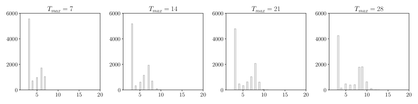
Figure 7: Empirical distribution of termination time $\tilde{T}$ for various maximum duration. This figure shows the histogram of the termination time $\tilde{T}$ for $T_{\max}\in\{7,14,21,28\}$ and $N=50$, based on 10,000 adaptive experiments. In PGAE, NTU and each set of ATU have $10$ and $20$ units, respectively. $\tau_{0}$ is chosen at the minus 10% of the average monthly flu occurrence rate, i.e., $\tau_{0}=-0.1(NT_{\max})^{-1}\sum_{i,s}Y_{is}(-1)$. The experiment termination threshold is $c=0.015\cdot N/\tau_{0}^{2}=13.83$. The results in this figure are robust to the choice of $c$, as shown in Figure LABEL:fig:experiment-termination-time-supp.

Finally, we note that there is a different trend in how the estimation error varies with $T_{\max}$ for different designs. For the benchmark design, the estimation error generally increases with $T_{\max}$. This is because as $T_{\max}$ increases, the benchmark design deviates more from the oracle design. For the oracle design, the estimation error consistently decreases with $T_{\max}$. This is because $\tilde{T}$ tends to increase with $T_{\max}$, as shown in Figure 7, and as a result, the precision of $\hat{\tau}_{0}$ using the oracle design increases with $\tilde{T}$. For the adaptive design, since the algorithm stops as the estimated precision reaches the fixed threshold $c$, we expect the estimation error to generally stay flat for various $T_{\max}$. But since the precision estimation is not exact, and is actually a conservative one, there is no specific pattern for fluctuations in the estimation error.

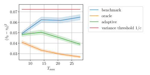
Figure 8: Comparison of various designs in adaptive experiments. This figure shows the mean and 95% confidence band of $(\hat{\tau}_{0}-\tau_{0})^{2}$ for adaptive, benchmark, and oracle designs, based on 10,000 synthetic adaptive experiments. As the precision threshold is $c=13.83$, the corresponding variance threshold $\mathrm{Var}(\hat{\tau})$ is $1/c=0.072$. The results in this figure are robust to the choice of $c$, as shown in Figure LABEL:fig:experiment-termination-time-supp.

6 Concluding Remarks

In this paper, we study the optimal design of staggered rollout experiments. These experiments are particularly useful for studying the impact of treatments that have causal effects on both current and future outcomes. Our goal is to optimally make treatment decisions for every unit at every time period, in anticipation of most precisely estimating the average instantaneous and lagged effects. This optimization problem can reduce the sample size requirement and directly minimize the opportunity cost of the experiment in practice. We first study the non-adaptive experiments, where the sample size is fixed and treatment decisions are made pre-experiment. We provide a near-optimal solution to the optimization problem. We further study adaptive experiments, where the experiments can be stopped early if needed. We propose the Precision-Guided Adaptive Experimentation (PGAE) algorithm for adaptive experiments. PGAE makes adaptive treatment decisions and allows for valid post-experiment inference. Finally, synthetic experiments on multiple data sets show that our proposed solutions for non-adaptive and adaptive experiments reduce the opportunity cost of the experiments by over 50%, compared to non-adaptive design benchmarks.

E-Companion

Table 1: Mathematical notations.

Notation	Description
$[M]$	$\{1,2,\cdots,M\}$ for any positive integer $M$
$\bm{x}_{a:b}$	$(x_{a},\ldots,x_{b})$ for integers $a$ and $b$, $1\leq a<b\leq n$
$\tau_{0}$	average instantaneous effect
$\tau_{j}$	average $j$-th period lagged effect
$\bm{\tau}$	$\begin{pmatrix}\tau_{\ell}&,&\cdots,&\tau_{0}\end{pmatrix}$
$\mathbf{y}_{t}$	$\big{(}Y_{1t},Y_{2t},\cdots,Y_{Nt}\big{)}^{\top}\in\mathbb{R}^{N\times 1}$
$\mathbf{z}_{t}$	$\big{(}z_{1t},z_{2t},\cdots,z_{Nt}\big{)}^{\top}\in\{-1,1\}^{N\times 1}$
$\bm{y}$	$\big{(}\mathbf{y}_{1}^{\top},\mathbf{y}_{2}^{\top},\cdots,\mathbf{y}_{T}^{\top}\big{)}^{\top}\in\mathbb{R}^{NT\times 1}$
$\bm{z}$	$\big{(}\mathbf{z}_{1}^{\top},\mathbf{z}_{2}^{\top},\cdots,\mathbf{z}_{T}^{\top}\big{)}^{\top}\in\mathbb{R}^{NT\times 1}$
$Y$	$\big{(}\mathbf{y}_{1},\mathbf{y}_{2},\cdots,\mathbf{y}_{T}\big{)}\in\mathbb{R}^{N\times T}$
$Z$	$\big{(}\mathbf{z}_{1},\mathbf{z}_{2},\cdots,\mathbf{z}_{T}\big{)}\in\{-1,1\}^{N\times T}$
$\omega_{t}$	equals $N^{-1}\sum_{i=1}^{N}z_{it}$
$\zeta_{i}$	equals $T^{-1}\sum_{t=1}^{T}z_{it}$
$A_{i}$	first time that unit $i$ adopts the treatment, $A_{i}\in[T]\cup\{\infty\}$
$A$	$(A_{1},\cdots,A_{N}^{\top})$
$\alpha_{i}$	unobserved unit fixed effect
$\beta_{t}$	unobserved time fixed effect
$\mathbf{X}_{i}$	observed covariates of dimension $d_{x}$
$\mathbf{u}_{i}$	observed covariates of dimension $d_{u}$
$\bm{\theta}_{t}$	unobserved coefficients of $\mathbf{X}_{i}$ at time $t$
$\mathbf{u}_{t}$	unobserved coefficients of $\mathbf{v}_{t}$ at time $t$
$\varepsilon_{it}$	residual of unit $i$ at time $t$
$\sigma_{\varepsilon}^{2}$	equals $\mathbb{E}[\varepsilon^{2}_{it}]$
$\xi_{\varepsilon}^{2}$	equals $\mathbb{E}[(\varepsilon^{2}_{it}-\sigma_{\varepsilon}^{2})^{2}]$
$e_{it}$	equals $\varepsilon_{it}+\mathbf{u}_{i}^{\top}\mathbf{v}_{t}$
$\bm{1}_{N}$	a vector of all ones of dimension $N$
$\mathbf{I}_{N}$	identity matrix of dimension $N\times N$
$\hat{\tau}_{j}$	estimate of $\tau_{j}$
$\hat{\bm{\tau}}$	estimate of $\bm{\tau}$
$\xrightarrow{d}$	convergence in distribution
$\xrightarrow{p}$	convergence in probability
For a set of random variables $\tilde{X}_{n}$ and constants $a_{n}$,
$\tilde{X}_{n}=O_{p}(a_{n})$	the set of values $\tilde{X}_{n}/a_{n}$ is stochastically bounded
$\tilde{X}_{n}=o_{p}(a_{n})$	the set of values $\tilde{X}_{n}/a_{n}$ converges to zero in probability
$A\mathrm{Cov}$	asymptotic covariance

7 Supplementary Material for Non-Adaptive Experiments

7.1 Supplementary Material for Generalized Least Squares

GLS estimates $\tau_{0},\cdots,\tau_{\ell}$, $\alpha_{i}$, $\beta_{t}$, and $\bm{\theta}_{t}$ in (1) by solving the following optimization problem

$$\min_{\bm{\tau},\bm{\alpha},\bm{\beta}_{(\ell+1):T},\bm{\theta}_{(\ell+1):T}}\quad \sum_{t=\ell+1}^{T}\bm{e}_{t}^{\top}\cdot\mathbf{W}^{-1}\cdot\bm{e}_{t}$$ (14)

$$\mathrm{s.t.}\quad \bm{e}_{t}=\mathbf{y}_{t}-\bm{\alpha}-\beta_{t}\cdot\bm{1}_{N}-\mathbf{X}\bm{\theta}_{t}-\tau_{0}\cdot\mathbf{z}_{t}-\cdots-\tau_{\ell}\cdot\mathbf{z}_{t-\ell}$$

$$\alpha_{i}=0\text{ for }i>N-d_{x}-1$$

where $\bm{\alpha}=\begin{pmatrix}\alpha_{1},&\cdots,&\alpha_{N}\end{pmatrix}$, $\bm{\beta}_{(\ell+1):T}=\begin{pmatrix}\beta_{\ell+1},&\cdots,&\beta_{T}\end{pmatrix}$, $\bm{\theta}_{(\ell+1):T}=\begin{pmatrix}\begin{array}[]{c|c|c}\bm{\theta}_{\ell+1}&\cdots&\bm{\theta}_{T}\end{array}\end{pmatrix}$, $\mathbf{X}=\begin{pmatrix}\begin{array}[]{c|c|c|c}\mathbf{X}_{1}&\mathbf{X}_{2}&\cdots&\mathbf{X}_{N}\end{array}\end{pmatrix}^{\top}\in\mathbb{R}^{N\times d_{x}}$, and $\mathbf{W}$ is a positive definite weighting matrix. The solution to (14) is denoted as $\big{(}\hat{\bm{\tau}},\hat{\bm{\alpha}},\hat{\bm{\beta}}_{(\ell+1):T},\hat{\bm{\theta}}_{(\ell+1):T}\big{)}$. In (14), we use observed outcomes from time $\ell+1$ to $T$, because these are the time periods that we have access to the current and past $\ell$ periods’ treatment assignments. The second constraint, $\alpha_{i}$ is equal to zero for the last $d_{x}+1$ units, ensures that all parameters can be uniquely identified. Below we provide a few special cases of how the estimation problem is simplified when a simpler specification is used.

Example 7.1 (No latent covariates)

If there are no latent covariates ($d_{u}=0$) in (1), then the optimal $\mathbf{W}$ is proportional to $\mathbf{I}_{N}$. The objective function in (14) is then simplified to $\sum_{t=\ell+1}^{T}\mathbf{e}_{t}^{\top}\mathbf{e}_{t}$, which is the case where GLS and ordinary least squares (OLS) coincide.

Example 7.2 (No observed covariates)

If there are no observed covariates ($d_{x}=0$), then the two constraints in (14) are simplified to $\bm{e}_{t}=\mathbf{y}_{t}-\bm{\alpha}-\beta_{t}\cdot\bm{1}_{N}-\tau_{0}\cdot\mathbf{z}_{t}-\cdots-\tau_{\ell}\cdot\mathbf{z}_{t-\ell}$ and only $\alpha_{N}$ is enforced to be $0$.

Example 7.3 (No time or unit fixed effects)

If (1) does not include time fixed effects, then the two constraints in (14) are simplified to $\bm{e}_{t}=\mathbf{y}_{t}-\bm{\alpha}-\mathbf{X}\bm{\theta}_{t}-\tau_{0}\cdot\mathbf{z}_{t}-\cdots-\tau_{\ell}\cdot\mathbf{z}_{t-\ell}$ and $\alpha_{i}=0\text{ for }i>N-d_{x}$. If (1) does not include unit fixed effects, then (14) only has one constraint, that is, $\bm{e}_{t}=\mathbf{y}_{t}-\beta_{t}\cdot\bm{1}_{N}-\mathbf{X}\bm{\theta}_{t}-\tau_{0}\cdot\mathbf{z}_{t}-\cdots-\tau_{\ell}\cdot\mathbf{z}_{t-\ell}$.

When (1) has latent covariates ($d_{u}>0$), the optimal $\mathbf{W}$ is proportional to the inverse covariance matrix of $\bm{e}_{t}$, which is $\big{(}\mathbf{U}\mathbf{\Sigma}_{v}\mathbf{U}^{\top}+\sigma_{\varepsilon}^{2}\mathbf{I}_{N}\big{)}^{-1}$ under Assumption 3.1 below and $\mathbf{U}=\begin{pmatrix}\begin{array}[]{c|c|c|c}\mathbf{u}_{1}&\mathbf{u}_{2}&\cdots&\mathbf{u}_{N}\end{array}\end{pmatrix}^{\top}\in\mathbb{R}^{N\times d_{u}}$. As $\mathbf{U}$, $\mathbf{\Sigma}_{v}$, and $\sigma_{\varepsilon}^{2}$ are unknown in practice, we can use feasible generalized least squares (FGLS). FGLS first solves (14) using identity matrix as the weighting matrix, then estimates $\mathbf{U}$, $\mathbf{\Sigma}_{v}$, and $\sigma_{\varepsilon}^{2}$, and lastly uses $\big{(}\hat{\mathbf{U}}\hat{\mathbf{\Sigma}}_{v}\hat{\mathbf{U}}^{\top}+\hat{\sigma}_{\varepsilon}^{2}\mathbf{I}_{N}\big{)}^{-1}$ as the weighting matrix to solve (14) again.

Lemma 7.4 (Gauss-Markov Theorem)

Consider a linear model $\bm{y}=\mathbf{X}\bm{\beta}+\text{noise}$ with $\mathbb{E}[\text{noise}\mid\mathbf{X}]=0$ and $\textnormal{Cov}[\text{noise}\mid\mathbf{X}]=\bm{\Omega}$. If $\bm{\Omega}=\sigma^{2}\bm{I}$, then the ordinary least squares estimator $\hat{\bm{\beta}}=(\mathbf{X}^{\top}\mathbf{X})^{-1}\mathbf{X}^{\top}\bm{y}$ is the best linear unbiased estimator (BLUE). Otherwise, when $\bm{\Omega}$ is not a multiple of the identity matrix, the generalized least squares estimator $\hat{\bm{\beta}}=(\mathbf{X}^{\top}\bm{\Omega}^{-1}\mathbf{X})^{-1}\mathbf{X}^{\top}\bm{\Omega}^{-1}\bm{y}$ is BLUE. Here, “best” means the estimator has the lowest variance among all unbiased linear estimators.

7.2 Supplementary Material for Theorem 3.8

The $a^{(\ell)}$ in Theorem 3.8 is defined as

$$a^{(\ell)}=(M^{(\ell)})^{-1}b^{(\ell)},$$

where $M^{(\ell)}$ and $b^{(\ell)}$ are defined as

$$M^{(\ell)}= \begin{bmatrix}\lfloor\ell/2\rfloor+1\\ &\lfloor\ell/2\rfloor+2\\ &&\ddots\\ &&&\ell\end{bmatrix}-\frac{1}{T-\ell}\begin{bmatrix}\ell-\lfloor\ell/2\rfloor&\ell-1-\lfloor\ell/2\rfloor&\ell-2-\lfloor\ell/2\rfloor&\cdots&1\\ \ell-1-\lfloor\ell/2\rfloor&\ell-1-\lfloor\ell/2\rfloor&\ell-2-\lfloor\ell/2\rfloor&\cdots&1\\ \vdots&\vdots&\vdots&\ddots&\vdots\\ 1&1&1&\cdots&1\end{bmatrix}$$ (15)

$$b^{(\ell)}= -\begin{bmatrix}\lfloor\ell/2\rfloor+1\\ \vdots\\ \ell-1\\ \ell\end{bmatrix}+\frac{1}{T-\ell}\begin{bmatrix}(\lfloor\ell/2\rfloor+1)^{2}\\ \vdots\\ (\ell-1)^{2}\\ \ell^{2}\end{bmatrix}-\frac{1}{T-\ell}\begin{bmatrix}\sum_{l=1}^{\ell-\lfloor\ell/2\rfloor}(\lfloor\ell/2\rfloor+1-l)\\ \vdots\\ 2\lfloor\ell/2\rfloor-1\\ \lfloor\ell/2\rfloor\end{bmatrix}$$ (16)

Below we provide the expression of $\omega_{\ell,t}^{\ast}$ for $\ell=3$, which has five stages. The example below complements the examples of $\omega_{\ell,t}^{\ast}$ for $\ell=0,1$ and $2$ in Examples 3.7, 3.15 and 3.16.

Example 7.5 ($\ell=3$)

In Theorem 3.8, $\omega^{\ast}_{\ell,t}$ takes the form of

$$\omega_{1}^{\ast}=-1,\quad\omega_{2}^{\ast}=-1+\frac{6}{6T^{2}-44T+79},\quad\omega_{3}^{\ast}=-1+\frac{12(T-4)}{6T^{2}-44T+79},$$

$$\omega_{t}^{\ast}=-1+\frac{2t-4}{T-3}\,\,\text{ for }t=4,\cdots,T-3,$$

$$\omega_{T-2}^{\ast}=1-\frac{12(T-4)}{6T^{2}-44T+79},\quad\omega_{T-1}^{\ast}=1-\frac{6}{6T^{2}-44T+79},\quad\omega_{T}^{\ast}=1.$$

7.3 D-Optimal Treatment Design

We consider the D-optimal design that minimizes the determinant of $\mathrm{Var}(\hat{\bm{\tau}})$. Note that $\mathrm{Var}(\hat{\bm{\tau}})=\mathrm{Prec}(\hat{\bm{\tau}})^{-1}$ and $\det(\mathrm{Var}(\hat{\bm{\tau}}))=1/\det(\mathrm{Prec}(\hat{\bm{\tau}})^{-1})$. Minimizing $\mathrm{Var}(\hat{\bm{\tau}})$ is equivalent to minimizing $1/\det(\mathrm{Prec}(\hat{\bm{\tau}}))$ and equivalent to:

$$\min_{\{A_{i}\}_{i\in[N]}}-\det\big{(}\mathrm{Prec}(\hat{\bm{\tau}})\big{)}.$$ (17)

Below we consider solving (17) for the specification $Y_{it}=\alpha_{i}+\beta_{t}+\tau_{0}z_{it}+\tau_{1}z_{i,t-1}+\cdots+\tau_{\ell}z_{i,t-\ell}+\varepsilon_{it}$. If the specification has covariates (either $d_{x}>0$ or $d_{u}>0$), then the role of covariates in the optimality conditions of (17) is identical to that for the T-optimal design in Theorem 3.8.

To solve (17), we first need to write every entry in $\mathrm{Prec}(\hat{\bm{\tau}})$ as a function of $z_{it}$:

$$\mathrm{Prec}(\hat{\bm{\tau}})_{jm}=\begin{cases}-\frac{N}{\sigma_{\varepsilon}^{2}}\left[\sum_{t=j}^{T-\ell-1+j}\omega_{t}^{2}-\frac{1}{T-\ell}\left(\sum_{t=j}^{T-\ell-1+j}\omega_{t}\right)^{2}+\frac{T-\ell}{2}\sum_{t=1}^{T}(\upsilon_{T+1-t}^{(j,j)}-\upsilon_{T-t}^{(j,j)})\omega_{t}\right]&j=m\\ -\frac{N}{\sigma_{\varepsilon}^{2}}\left[\sum_{t=j}^{T-\ell-1+j}\omega_{t}\omega_{t+m-j}-\frac{1}{T-\ell}\left(\sum_{t=j}^{T-\ell-1+j}\omega_{t}\right)\left(\sum_{t=m}^{T-\ell-1+m}\omega_{t}\right)\right.\\ \quad\left.+\frac{T-\ell}{2}\sum_{t=1}^{T}(\upsilon_{T+1-t}^{(j,m)}-\upsilon_{T-t}^{(j,m)})\omega_{t}-\sum_{t=j}^{m-1}(\omega_{t}-\omega_{T-\ell+t})\right]&j<m\\ \mathrm{Prec}(\hat{\bm{\tau}})_{mj}&j>m\\ \end{cases}$$ (18)

where $\omega_{t}=\frac{1}{N}\sum_{i=1}^{N}z_{it}$ and $\upsilon_{t}^{(j,m)}$ is defined as

$$\upsilon_{t}^{(j,m)}=\begin{cases}1&t\leq\ell+1-m\\ -\left(-1+\frac{2(t-1-\ell+m)}{T-\ell}\right)&\ell+1-m<t\leq\ell+1-j\\ \left(-1+\frac{2(t-1-\ell+m)}{T-\ell}\right)\left(-1+\frac{2(t-1-\ell+j)}{T-\ell}\right)&\ell+1-j<t\leq T+1-m\\ \left(-1+\frac{2(t-1-\ell+j)}{T-\ell}\right)&T+1-m<t\leq T+1-j\\ 1&T+1-j<t\\ \end{cases}$$

Note that each entry in $\mathrm{Prec}(\hat{\bm{\tau}})$ is a quadratic function of $\omega_{t}$. Based on the Leibniz formula for determinants, $\det\big{(}\mathrm{Prec}(\hat{\bm{\tau}})\big{)}$ is a linear combination of $2(\ell+1)$ products of $\ell+1$ distinct elements in $\mathrm{Prec}(\hat{\bm{\tau}})$ (recall that $\mathrm{Prec}(\hat{\bm{\tau}})$ is an $(\ell+1)\times(\ell+1)$ matrix. Therefore, $\mathrm{Prec}(\hat{\bm{\tau}})$ is the $2(\ell+1)$-th degree polynomial function of $z_{it}$.

It is generally infeasible to analytically solve (17) for $\ell>1$. We therefore use the off-the-shelf software to find the optimal $\omega_{t}$. We show the optimal solution to (17) for $T=10$ in Figure 9. Similar to the T-optimal design, the optimal $\omega_{t}$ is symmetric with respect to the center (i.e., $((T+1)/2,0)$). Also similar to the T-optimal design, if $\ell$ is larger, then the optimal $\omega_{t}$ is generally smaller at the beginning, increases at a faster rate in the middle, and is generally larger in the end.

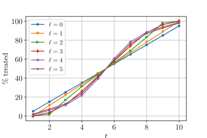
Figure 9: D-optimal treatment design: Optimal treated proportion ($(1+\omega_{t})/2$) at each period for a $T$-period treatment design and various $\ell$, where $T=10$. Different colors represent different $\ell$.

7.4 Reversible Treatment Adoption Case

There are two ways to look at the reversible treatment adoption case: first, each unit is treated at most once; second, units can be treated more than once. Surprisingly, the first case is a special case of the irreversible pattern introduced in Section 2, as shown in 7.4.1. For the second case, we derive analogous results as those for the irreversible pattern in 7.4.2.

7.4.1 Equivalent Representation of One-time Treatment

For the one-time treatment, such as the participation of a job-training or skill-improvement program, we can still use specification (1) to estimate how the effect of this one-time treatment varies with the time. However, we need to use a different definition of $z_{it}$ in specification (1): $z_{it}=+1$ denotes that unit $i$ has been treated up to time $t$, and $z_{it}=-1$ denotes otherwise.

An alternative approach is to use the definition of treatment variable as in the main text: Let $w_{it}=\{0,1\}$ denote whether unit $i$ is treated at time $t$ ($w_{it}=1$) or not ($w_{it}=0$). In the case of one-time treatment, at most one of $w_{it},\cdots,w_{i,t-\ell}$ is $1$. Consider the following specification using $w_{it}$:

$$Y_{it}=\tilde{\alpha}_{i}+\tilde{\beta}_{t}+\mathbf{X}_{i}^{\top}\bm{\theta}_{t}+\mathbf{u}_{i}^{\top}\mathbf{v}_{t}+\tilde{\tau}_{0}w_{it}+\tilde{\tau}_{1}w_{i,t-1}+\cdots+\tilde{\tau}_{\ell}w_{i,t-\ell}+\varepsilon_{it}\,.$$ (19)

$\tilde{\tau}_{j}$ can be interpreted as the treatment effect given that a unit was treated $j$-period ago. If $|\tilde{\tau}_{\ell}|<\cdots<|\tilde{\tau}_{1}|<|\tilde{\tau}_{0}|$, then the effect of the one-time treatment attenuates over time.

We can show that specification (19) using $w_{it}$ is equivalent to specification (1) using $z_{it}$ with the change of variables:

$$\tilde{\tau}_{j}=2\sum_{k=0}^{j}\tau_{k}\qquad\tilde{\alpha}_{i}=\alpha_{i}-\sum_{k=0}^{\ell}\tau_{k}\qquad\tilde{\beta}_{t}=\beta_{t}.$$

7.4.2 General Reversible Treatment Pattern

Next we consider the case where a unit can arbitrarily switch between treatment and control (i.e., Assumption 2 is violated). Below we provide the optimality conditions of T-optimal design for this case.

Proposition 7.6

Suppose Assumption 1 holds, and the treatment is reversible. Let $\omega_{t}=\sum_{i=1}^{N}z_{it}/N$ and $\zeta_{i}=\sum_{i=1}^{T}z_{it}/T$.

1. Suppose $\tau$ is estimated from the least squares estimator under the specification $Y_{it}=\beta_{t}+\tau z_{it}+\varepsilon_{it}$. If $\varepsilon_{it}$ is i.i.d. in $i$ and $t$ with mean $0$ and variance $\sigma_{\varepsilon}^{2}$, then any treatment design is optimal if it satisfies

   $$\omega_{t}=0.$$

2. Suppose $\tau$ is estimated from the least squares estimator under the specification $Y_{it}=\alpha_{i}+\tau z_{it}+\varepsilon_{it}$. If $\varepsilon_{it}$ is i.i.d. in $i$ and $t$ with mean $0$ and variance $\sigma_{\varepsilon}^{2}$, then any treatment design is optimal if it satisfies

   $$\zeta_{i}=0.$$

3. Suppose $\tau$ is estimated from the least squares estimator under the specification $Y_{it}=\alpha_{i}+\beta_{t}+\tau z_{it}+\varepsilon_{it}$. If $\varepsilon_{it}$ is i.i.d. in $i$ and $t$ with mean $0$ and variance $\sigma_{\varepsilon}^{2}$, then any treatment design is optimal if it satisfies

   $$\omega_{t}=0,\quad\zeta_{i}=0.$$

4. Suppose $\tau$ is estimated from the least squares estimator under the specification $\alpha_{i}+\beta_{t}+\mathbf{X}^{\top}_{i}\bm{\theta}_{t}+\mathbf{u}^{\top}_{i}\mathbf{v}_{t}+\tau_{0}z_{it}+\tau_{1}z_{i,t-1}+\cdots+\tau_{\ell}z_{i,t-\ell}+\varepsilon_{it}$ for $\ell\geq 0$. Suppose the assumptions in Theorem 3.8 hold, and both $\mathbf{X}_{i}$ and $\mathbf{u}_{i}$ are discrete-valued. Let $\omega_{g,t}=\frac{1}{|\mathcal{O}_{g}|}\sum_{i\in\mathcal{O}_{g}}z_{it}$, where $\mathcal{O}_{g}=\{i:X_{i}=x_{g},u_{i}=u_{0,g}\}$. Any treatment design is optimal if it satisfies

   $$\omega_{g,t}=0,\,\text{ for all $t$ and $g$},\quad\zeta_{i}^{(j)}=0,\,\text{ for all $i$ and $j$},$$

   where $\zeta_{i}^{(j)}=\sum_{t=j}^{T-\ell+j-1}z_{it}/(T-\ell)$

Proof 7.7

Proof of Proposition 7.6

1. Under the specification $Y_{it}=\beta_{t}+\tau z_{it}+\varepsilon_{it}$, the precision of $\hat{\tau}$ equals

   $$\mathrm{Prec}(\hat{\tau})=NT-N\sum_{t=1}^{T}\omega_{t}^{2}.$$

   The precision is maximized at $\omega_{t}=0$.

2. Under the specification $Y_{it}=\alpha_{i}+\tau z_{it}+\varepsilon_{it}$, the precision of $\hat{\tau}$ equals

   $$\mathrm{Prec}(\hat{\tau})=NT-T\sum_{i=1}^{N}\zeta_{i}^{2}.$$

   The precision is maximized at $\zeta_{i}=0$.

3. Under the specification $Y_{it}=\alpha_{i}+\beta_{t}+\tau z_{it}+\varepsilon_{it}$, from the proof of Lemma 7.9, the precision of $\hat{\tau}$ equals

   $$\mathrm{Prec}(\hat{\tau})=NT-\left(T\sum_{i=1}^{N}\zeta_{i}^{2}-\frac{N}{T}\left(\sum_{t=1}^{T}\omega_{t}\right)^{2}+N\sum_{t=1}^{T}\omega_{t}^{2}\right).$$

   The precision is maximized at $\zeta_{i}=0$ and $\omega_{t}=0$, given that $\sum_{t=1}^{T}\omega_{t}^{2}-\frac{1}{T}\left(\sum_{t=1}^{T}\omega_{t}\right)^{2}$ is minimized at $\omega_{t}=0$.

4. Under the specification $Y_{it}=\alpha_{i}+\beta_{t}+\mathbf{X}^{\top}_{i}\bm{\theta}_{t}+\mathbf{u}^{\top}_{i}\mathbf{v}_{t}+\tau_{0}z_{it}+\tau_{1}z_{i,t-1}+\cdots+\tau_{\ell}z_{i,t-\ell}+\varepsilon_{it}$, the role of observed and latent covariates in the optimal design is the same as that in Theorem 3.8. The major difference with Theorem 3.8 is the optimal treated fraction conditions. Note that the precision matrix $\mathrm{Prec}(\hat{\bm{\tau}})$ takes the form of (see Equation (24)),

   $$\mathrm{Prec}\left(\hat{\bm{\tau}}\right)=\bm{Z}_{\ell}^{\top}\bm{\Sigma}^{-1}_{e}(\bm{\Sigma}_{e}-\bm{\Gamma}(\bm{\Gamma}^{\top}\bm{\Sigma}^{-1}_{e}\bm{\Gamma})^{-1}\bm{\Gamma}^{\top})\bm{\Sigma}^{-1}_{e}\bm{Z}_{\ell}$$

   where the $(j,j)$-th entry (i.e., diagonal entry) in $\mathrm{Prec}\left(\hat{\bm{\tau}}\right)$ takes the form of (see Equations (25) and (26) in Lemma 8.1, and the proof of Lemma 7.9)

   $$N(T-\ell)-\Bigg{[}N\sum_{t=j}^{T-\ell+j-1}\omega_{t}^{2}-\frac{N}{T-\ell}\left(\sum_{t=j}^{T-\ell+j-1}\omega_{t}\right)^{2}+(T-\ell)\sum_{i=1}^{N}(\zeta_{i}^{(j)})^{2}\Bigg{]}$$

   $$-\frac{N}{\sigma_{\varepsilon}^{2}}\sum_{j=1}^{\ell+1}f_{j,\mathbf{X}}(Z)-\frac{N}{\sigma_{\varepsilon}^{2}}\sum_{j=1}^{\ell+1}f_{j,\mathbf{U}}(Z)$$

   $f_{j,\mathbf{X}}(Z)$ and $f_{j,\mathbf{U}}(Z)$ are defined in Lemma 7.9. The $(j,j)$-th entry in $\mathrm{Prec}(\hat{\bm{\tau}})$ is maximized at $\omega_{t}=0$ for all $t$ and $\zeta_{i}^{(j)}=0$ for all $i$. Moreover both $f_{j,\mathbf{X}}(Z)$ and $f_{j,\mathbf{U}}(Z)$ are minimized at $\omega_{g,t}=0$. The T-optimal design maximizes the trace of the precision matrix, which is satisfied by the solution provided in Lemma 7.6.4.

We conclude the proof of Lemma 7.6.

7.5 A Rounding Approach for A Feasible Solution

When there does not exist a feasible solution in $\mathbb{A}^{\mathrm{disc}}_{\mathrm{opt}}$, we suggest using the nearest integer rounding rule as follows to obtain a feasible $\{A_{i}\}_{i\in[N]}$.

Nearest integer rounding rule: If the number of treated units for each stratum suggested by Theorem 3.8, i.e., is not an integer,

$$\frac{|\mathcal{O}_{g}|(1+\omega_{\ell,t}^{\ast})}{2T}$$

we suggest rounding it to an integer using the nearest integer rule. We separate the number of treated units into the integer and decimal parts

$$\frac{|\mathcal{O}_{g}|(1+\omega_{\ell,t}^{\ast})}{2T}=\underbrace{\lfloor\frac{|\mathcal{O}_{g}|(1+\omega_{\ell,t}^{\ast})}{2T}\rfloor}_{N_{\mathrm{treated},g,t}^{\mathrm{int}}}+\underbrace{\frac{|\mathcal{O}_{g}|(1+\omega_{\ell,t}^{\ast})}{2T}-\lfloor\frac{|\mathcal{O}_{g}|(1+\omega_{\ell,t}^{\ast})}{2T}\rfloor}_{N_{\mathrm{treated},g,t}^{\mathrm{dec}}}$$

The nearest integer rounding rule works as follows

• If the decimal part $N_{\mathrm{treated},g,t}^{\mathrm{dec}}<0.5$, or if $N_{\mathrm{treated},g,t}^{\mathrm{dec}}=0.5$ with $t<T/2$, then the rounded number of treated units is

  $$\frac{1}{|\mathcal{O}_{g}|}\sum_{i\in\mathcal{O}_{g}}\bm{1}_{A^{\textnormal{rnd}}_{i}\leq t}=N_{\mathrm{treated},g,t}^{\mathrm{int}}$$

• Otherwise, the rounded number of treated units is

  $$\frac{1}{|\mathcal{O}_{g}|}\sum_{i\in\mathcal{O}_{g}}\bm{1}_{A^{\textnormal{rnd}}_{i}\leq t}=N_{\mathrm{treated},g,t}^{\mathrm{int}}+1$$

Let $Z^{\textnormal{rnd}}$ be the treatment design satisfying the rounded number of treated units for each stratum. Let $Z^{\mathrm{int}\ast}$ be the optimal integer solution to optimization problem (2). $\mathrm{tr}\big{(}\mathrm{Prec}(\hat{\bm{\tau}})\big{)}_{Z}$ be the objective function (2) (i.e. $\mathrm{tr}\big{(}\mathrm{Prec}(\hat{\bm{\tau}})\big{)}$) evaluated at $Z$.

The following proposition bounds the difference between $\mathrm{tr}\big{(}\mathrm{Prec}(\hat{\bm{\tau}})\big{)}_{Z^{\textnormal{rnd}}}$ and $\mathrm{tr}\big{(}\mathrm{Prec}(\hat{\bm{\tau}})\big{)}_{Z^{\mathrm{int}^{\ast}}}$.

Proposition 7.8

Suppose the assumptions in Theorem 3.8 hold, $d_{u}=0$ and $N$ is even, and $x_{k,\max}=\max_{g}|x_{gk}|$ is finite, where $x_{gk}$ is the $k$-th coordinate of $x_{g}$ for all strata $g$. We have

$$\mathrm{tr}\big{(}\mathrm{Prec}(\hat{\bm{\tau}})\big{)}_{Z^{\textnormal{rnd}}}=\mathrm{tr}\big{(}\mathrm{Prec}(\hat{\bm{\tau}})\big{)}_{Z^{\mathrm{int}\ast}}\cdot\left(1+O\left(\frac{1+\sum_{k=1}^{d_{x}}x_{k,\max}^{2}}{N^{2}_{\min}}\right)\right).$$

Since the probability of each realization of $\mathbf{X}_{i}$ is bounded away from 0 and $x_{k,\max}$ is finite, we have $O\left((1+\sum_{k=1}^{d_{x}}x_{k,\max}^{2})/N^{2}_{\min}\right)=O\left(1/N^{2}\right)$ as $N\rightarrow\infty$. However, if $G$ is large compared with $N$ (or $\mathbf{X}_{i}$ takes infinitely many values), $\mathrm{tr}\big{(}\mathrm{Prec}(\hat{\bm{\tau}})\big{)}_{Z^{\textnormal{rnd}}}$ could be much larger than $\mathrm{tr}\big{(}\mathrm{Prec}(\hat{\bm{\tau}})\big{)}_{Z^{\mathrm{int}\ast}}$. In this case, we could instead partition units into only a few (e.g., 2 or 3) groups based on their covariates’ values using $K$-means or some other methods. Within each group, the treated fraction conditions are satisfied.

7.6 Supplementary Details in Choosing a Treatment Design

In Algorithm 2, we provide a procedure to randomly choose a treatment design for each stratum based on the treated fraction conditions. If there are no covariates (in the outcome model), then this is the case where we only have one stratum that consists of all experimental units.

We want to highlight that Algorithm 2 allows for the case where the treatment fraction conditions in Theorem 3.8 can not be exactly satisfied for any treatment design. For this case, Algorithm 2 uses the nearest integer rounding algorithm in 7.5 in choosing a treatment design.

1 Inputs : $|\mathcal{O}_{g}|$, $[\omega_{\ell,t}^{\ast}]_{t\in[T]}$

2 for $t=1,\cdots,T$ do

      3 $N_{\mathrm{treated},g,t}^{\mathrm{int}}\leftarrow\lfloor|\mathcal{O}_{g}|(1+\omega_{\ell,t}^{\ast})/2\rfloor$

      4 $N_{\mathrm{treated},g,t}^{\mathrm{dec}}\leftarrow|\mathcal{O}_{g}|(1+\omega_{\ell,t}^{\ast})/2-N_{\mathrm{treated},g,t}^{\mathrm{int}}$

      5 if $N_{\mathrm{treated},g,t}^{\mathrm{dec}}<0.5$ or $N_{\mathrm{treated},g,t}^{\mathrm{dec}}=0.5$ with $t<T/2$ then

            6 $N_{g,t}\leftarrow N_{\mathrm{treated},g,t}^{\mathrm{int}}$

      else

            7 $N_{g,t}\leftarrow N_{\mathrm{treated},g,t}^{\mathrm{int}}+1$

            

       end if

      

end for

8$f(\cdot)\leftarrow$ a random function that shuffles $\{1,2,\cdots,|\mathcal{O}_{g}|\}$

9 $Z_{g}\leftarrow[-1]^{|\mathcal{O}_{g}|\times T}$

10 for $i=1,\cdots,|\mathcal{O}_{g}|$ do

      11 for $t=1,\cdots,T$ do

            12 if $f(i)\leq N_{g,t}$ then

                   $z_{g,it}\leftarrow 1$

                  

            else

                   $z_{g,it}=-1$

                  

             end if

            

       end for

      

end for

13return $Z_{g}$

Algorithm 2 Choose a treatment design for each stratum $g$

7.7 Latent Covariates

7.7.1 Estimation of latent covariates

If there are latent covariates, we suggest, whenever possible, using the historical control data for the same set of units in designing the experiment. This is because historical data has information about $\mathbf{u}_{i}$. Below we provide a heuristic approach to using historical data to find a better treatment design.

We can apply singular value decomposition (SVD) to the historical data and take the top singular vectors as the estimated $\mathbf{u}_{i}$, denoted as $\hat{\mathbf{u}}_{i}$. We can use cross-validation to choose the number of singular vectors. Specifically, we can partition the historical data in the time dimension into training and validation sets. Then we estimate the singular vectors on the training set, and design synthetic experiments on the validation set based on various numbers of singular vectors. Finally, we can select the optimal number of singular vectors whose experimental design has the lowest estimation error of treatment effects on the validation set.

We suggest using SVD with cross-validation for the following reason. Since the time horizon $T$ of the experiment is typically short (e.g., one flu season with $T=7$ in our empirical application, and short $T$ is the regime where statistical power is a concern), it is typically sufficient to account for the first one or two latent factors in the feasible GLS estimator. Then it is natural to account for the top a few latent factors in the design of experiments, where SVD with cross-validation seems to be a reasonable approach.

If historical data have missing observations, or if both the historical data and experimental data have a long time horizon (where it is reasonable to estimate more latent factors), then we could use low-rank matrix estimation with nuclear norm regularization to estimate latent covariates from the historical data.

7.7.2 Non-adaptive treatment design based on latent covariates

We can first estimate latent covariates by SVD from historical data, and then treat $\hat{\mathbf{u}}_{i}$ as “observed” covariates in the design of non-adaptive experiments. If $\hat{\mathbf{u}}_{i}$ is continuous, then we can partition units into strata based on $\hat{\mathbf{u}}_{i}$ by applying $k$-means clustering on the largest singular vectors, similar to observed continuous-valued covariates. Here the number of clusters $k$ can be chosen by cross-validation. Each cluster of units from $k$-means clustering is a stratum, and we can apply Algorithm 2 to randomly choose a treatment design for each stratum.

The approach of stratifying based on top singular vectors is conceptually similar to spectral clustering, which enjoys nice theoretical and empirical properties (see e.g., Ng et al. (2001)) and works well in our empirical applications. Admittedly, it is possible to stratify based on the ideas of other clustering algorithms (e.g., density-based clustering, mean-shift clustering), and we leave this for future work.

Note that it seems possible to use the currently available experimental data to improve the estimation precision of $\hat{\mathbf{u}}_{i}$ and treatment decisions for subsequent experimental periods. However, we do not pursue this route for two reasons.

First, if historical data does not have many periods, then $\hat{\mathbf{u}}_{i}$ can be quite noisy early in the experiment. We may not want to use noisy estimates of $\mathbf{u}_{i}$ for treatment decisions, because the mistakes we make in the early periods (due to very noisy estimates of $\mathbf{u}_{i}$) can carry over to later periods. We have verified this in numerical simulations but did not include them in the paper, given the paper is quite lengthy already.

Second, if historical data has many periods, which allows us to precisely estimate $\mathbf{u}_{i}$, then having a few more experimental periods can only marginally improve the precision of $\hat{\mathbf{u}}_{i}$ and treatment allocations. This is because the convergence rate of $\hat{\mathbf{u}}_{i}$ is $\sqrt{T}$ (Bai 2003).

7.8 Separable Quadratic Representation

In this subsection, we state a critical lemma that shows $\mathrm{tr}\left(\mathrm{Prec}(\hat{\bm{\tau}})\right)$ can be decomposed into three separable quadratic functions: the first one does not depend on $\mathbf{X}$ and $\mathbf{U}$, the second one only depends on $\mathbf{X}$, and the third one only depends on $\mathbf{U}$. The solutions to each of these three show the effects of fixed effects, observed covariates, and latent covariates on the optimal treatment assignments, respectively. If a solution simultaneously optimizes all three quadratic functions, then this solution is an optimal solution to (2).

Lemma 7.9 (Separable Quadratic Representation)

Suppose Assumptions 2, 1, and 3.1 hold. Suppose $\hat{\bm{\tau}}$ is estimated from the infeasible GLS with $\mathbf{W}=[w_{ij}]\propto\big{(}\mathbf{U}\mathbf{\Sigma}_{v}\mathbf{U}^{\top}+\sigma_{\varepsilon}^{2}\mathbf{I}_{N}\big{)}^{-1}$, rows in $\mathbf{X}$ and $\mathbf{U}$ are demeaned, that is, $\sum_{i=1}^{N}\mathbf{X}_{i}=\bm{0}_{d_{x}}$ and $\sum_{i=1}^{N}\mathbf{u}_{i}=\bm{0}_{d_{u}}$, $\sum_{i=1}^{N}\mathbf{X}_{i}\mathbf{u}_{i}^{\top}=\mathbf{0}_{d_{x},d_{u}}$, and $\mathbf{\Sigma}_{v}=\sigma_{\varepsilon}^{2}\cdot\mathbf{I}_{d_{u}}$. Let $T_{\ell}=T-\ell$ and $j_{\ell}=j+T_{\ell}-1$ for all $j$. Then $\mathrm{tr}\big{(}\mathrm{Prec}(\hat{\bm{\tau}})\big{)}$ takes the form of

$$\mathrm{tr}\big{(}\mathrm{Prec}(\hat{\bm{\tau}})\big{)}= -\frac{N}{\sigma_{\varepsilon}^{2}}\sum_{j=1}^{\ell+1}\bigg{(}\underbrace{(\bm{\omega}_{j:j_{\ell}})^{\top}\mathbf{P}_{\bm{1}_{T_{\ell}}}\bm{\omega}_{j:j_{\ell}}+2\bm{b}_{\ell}^{\top}\bm{\omega}_{j:j_{\ell}}}_{f_{j,\bm{1}}(Z)}+\underbrace{\textstyle\sum_{k=1}^{d_{x}}(\bm{\omega}_{j:j_{\ell}}^{x_{k}})^{\top}\mathbf{P}_{\bm{1}_{T_{\ell}}}\bm{\omega}_{j:j_{\ell}}^{x_{k}}}_{f_{j,\mathbf{X}}(Z)}+\underbrace{\textstyle\frac{1}{N}\bm{z}_{j:j_{\ell}}^{\top}\mathbf{M}_{\mathbf{U}}\bm{z}_{j:j_{\ell}}}_{f_{j,\mathbf{U}}(Z)}\bigg{)},$$ (20)

where $\bm{\omega}_{j:j_{\ell}}=\big{(}{\omega}_{j},\cdots,{\omega}_{j_{\ell}}\big{)}^{\top}$ with ${\omega}_{t}=\frac{1}{N}\sum_{i=1}^{N}z_{it}$, $\bm{\omega}_{j:j_{\ell}}^{x_{k}}=\big{(}{\omega}^{x_{k}}_{j},\cdots,{\omega}^{x_{k}}_{j_{\ell}}\big{)}^{\top}$ with ${\omega}^{x_{k}}_{t}=\frac{1}{N}\sum_{i=1}^{N}X_{ik}z_{it}$, $\bm{z}_{j:j_{\ell}}=\big{(}\mathbf{z}_{j}^{\top},\cdots,\mathbf{z}_{j_{\ell}}^{\top}\big{)}^{\top}\in\{-1,+1\}^{NT_{\ell}\times 1}$, $\mathbf{P}_{\bm{1}_{T_{\ell}}}=\mathbf{I}_{T_{\ell}}-\frac{1}{T_{\ell}}\bm{1}_{T_{\ell}}\bm{1}_{T_{\ell}}^{\top}$, $\mathbf{b}_{\ell}=[b_{\ell,t}]\in[-1,1]^{T_{\ell}}$ with $b_{\ell,t}=\frac{T_{\ell}+2-2t}{T_{\ell}}$, and $\mathbf{M}_{\mathbf{U}}=\mathbf{P}_{\bm{1}_{T_{\ell}}}\otimes\mathbf{U}(\mathbf{I}_{d_{u}}+\mathbf{U}^{\top}\mathbf{U})^{-1}\mathbf{U}^{\top}$.

From Lemma 7.9, maximizing $\mathrm{tr}\big{(}\mathrm{Prec}(\hat{\bm{\tau}})\big{)}$ is equivalent to

$$\min_{\{A_{i}\}_{i\in[N]}}\underbrace{\textstyle\sum_{j=1}^{\ell+1}f_{j,\bm{1}}(Z)}_{f_{\bm{1}}(Z)}+\underbrace{\textstyle\sum_{j=1}^{\ell+1}f_{j,\mathbf{X}}(Z)}_{f_{\mathbf{X}}(Z)}+\underbrace{\textstyle\sum_{j=1}^{\ell+1}f_{j,\mathbf{U}}(Z)}_{f_{\mathbf{U}}(Z)}.$$ (21)

If we can find an $\{A_{i}\}_{i\in[N]}$ that simultaneously minimizes each of $f_{\bm{1}}(Z)$, $f_{\mathbf{X}}(Z)$, and $f_{\mathbf{U}}(Z)$, then this $\{A_{i}\}_{i\in[N]}$ minimizes (21). In the following, we separately analyze the three sub-problems of (21): $\min_{\{A_{i}\}_{i\in[N]}}f_{\bm{1}}(Z)$, $\min_{\{A_{i}\}_{i\in[N]}}f_{\mathbf{X}}(Z)$, and $\min_{\{A_{i}\}_{i\in[N]}}f_{\mathbf{U}}(Z)$.

We first consider the sub-problem $\min_{\{A_{i}\}_{i\in[N]}}f_{\bm{1}}(Z)$. The solution to this problem characterizes the effect of the presence of two-way fixed effects, $\alpha_{i}$ and $\beta_{t}$ on the optimal treatment assignments. Note that $f_{\bm{1}}(Z)$ is a sum of quadratic and linear terms:

$$f_{\bm{1}}(Z)=\sum_{j=1}^{\ell+1}\big{(}(\bm{\omega}_{j:j_{\ell}})^{\top}\mathbf{P}_{\bm{1}_{T_{\ell}}}\bm{\omega}_{j:j_{\ell}}+2\bm{b}_{\ell}^{\top}\bm{\omega}_{j:j_{\ell}}\big{)}.$$ (22)

It is possible to provide the analytical solution to $\min_{\{A_{i}\}_{i\in[N]}}f_{\bm{1}}(Z)$ based on its first order condition. The analytical solution is provided in (4).

Next we consider the other two sub-problems: $\min_{\{A_{i}\}_{i\in[N]}}f_{\mathbf{X}}(Z)$ and $\min_{\{A_{i}\}_{i\in[N]}}f_{\mathbf{U}}(Z)$. The solution to these two problems characterizes the effects of the presence of $\mathbf{X}_{i}$ and/or $\mathbf{u}_{i}$ on the optimal treatment assignments, respectively. Note that both $f_{\mathbf{X}}(Z)$ and $f_{\mathbf{U}}(Z)$ are sums of quadratic functions of $\{\mathbf{z}_{t}\}_{t=1}^{T}$ that do not have linear terms. The Hessian of $f_{\mathbf{X}}(Z)$ and $f_{\mathbf{U}}(Z)$ are both semidefinite, following the definition of two matrices in $f_{\mathbf{X}}(Z)$ and $f_{\mathbf{U}}(Z)$, i.e., $\mathbf{P}_{\bm{1}_{T_{\ell}}}=\mathbf{I}_{T_{\ell}}-\frac{1}{T_{\ell}}\bm{1}_{T_{\ell}}\bm{1}_{T_{\ell}}^{\top}$ and $\mathbf{M}_{\mathbf{U}}=\mathbf{P}_{\bm{1}_{T_{\ell}}}\otimes\mathbf{U}(\mathbf{I}_{d_{u}}+\mathbf{U}^{\top}\mathbf{U})^{-1}\mathbf{U}^{\top}$. Then the minimum possible value of $f_{\mathbf{X}}(Z)$ and $f_{\mathbf{U}}(Z)$ is 0. As shown in Theorem 3.8 below, the minimum value of $f_{\mathbf{X}}(Z)$ can be achieved if $\{A_{i}\}_{i\in[N]}\in\mathbb{A}_{\mathbf{X}}$, and the minimum value of $f_{\mathbf{U}}(Z)$ can be achieved if $\{A_{i}\}_{i\in[N]}\in\mathbb{A}_{\mathbf{U}}$.

8 Proof of Results for Non-Adaptive Experiments

We can combine $\beta_{t}$ with $\bm{\theta}_{t}$ in the specification (1), that is,

$$Y_{it}=\alpha_{i}+\underbrace{\begin{bmatrix}1&\mathbf{X}^{\top}_{i}\end{bmatrix}}_{\tilde{\mathbf{X}}_{i}^{\top}}\begin{bmatrix}\beta_{t}\\ \bm{\theta}_{t}\end{bmatrix}+\tau_{0}z_{it}+\tau_{1}z_{i,t-1}+\cdots+\tau_{\ell}z_{i,t-\ell}+\underbrace{\mathbf{u}_{i}^{\top}\mathbf{v}_{t}+\varepsilon_{it}}_{e_{it}}.$$

Denote $p\coloneqq d_{x}+1$, and then $\tilde{\mathbf{X}}_{i}\in\mathbb{R}^{p}$. Denote $\zeta_{i}=\frac{1}{T}\sum_{t=1}^{T}z_{it}$ for all $i$ and $\tilde{\omega}_{t}=\frac{1}{N}\sum_{i=1}^{N}\tilde{\mathbf{X}}_{i}z_{it}\in\mathbb{R}^{p}$ for all $t$.

We write the potential outcomes from time $\ell+1$ to $T$ into a vectorized form, and then we have

$$\bm{y}_{(\ell+1):T}=\begin{bmatrix}\bm{z}_{1:(T-\ell)}&\cdots&\bm{z}_{\ell:(T-1)}&\bm{z}_{(\ell+1):T}&\bm{\Gamma}\end{bmatrix}\begin{bmatrix}\bm{\tau}\\ \bm{\alpha}_{1:(N-p)}\\ \bm{\beta}_{(\ell+1):T}\\ \bm{\theta}_{(\ell+1):T}\end{bmatrix}+\bm{e}_{(\ell+1):T},$$

where $\hat{\bm{\tau}}=\begin{pmatrix}\tau_{\ell}&,&\cdots,&\tau_{0}\end{pmatrix}$,

$$\bm{\Gamma}=\begin{bmatrix}\tilde{\mathbf{I}}_{N-p}&\bm{1}_{N}&\mathbf{X}&&&\\ \tilde{\mathbf{I}}_{N-p}&&&\bm{1}_{N}&\mathbf{X}&\\ \vdots&&&&&&\ddots\\ \tilde{\mathbf{I}}_{N-p}&&&&&&&&\bm{1}_{N}&\mathbf{X}\\ \end{bmatrix}=\begin{bmatrix}\tilde{\mathbf{I}}_{N-p}&\tilde{\mathbf{X}}\\ \tilde{\mathbf{I}}_{N-p}&&\tilde{\mathbf{X}}\\ \vdots&&&\ddots\\ \tilde{\mathbf{I}}_{N-p}&&&&\tilde{\mathbf{X}}\\ \end{bmatrix}\in\mathbb{R}^{(N(T-\ell))\times(N+(T-\ell-1)p)},$$

$\tilde{\mathbf{I}}_{N-p}=\begin{bmatrix}\mathbf{I}_{N-p}&\mathbf{0}_{N-p,p}\end{bmatrix}^{\top}\in\mathbb{R}^{N\times(N-p)}$, $\mathbf{I}_{N-p}$ is an identity matix of dimension $(N-p)\times(N-p)$ and $\mathbf{0}_{N-p,p}$ is a matrix of $0$. Note that we restrict $\bm{\alpha}_{(N-p+1):N}=0$ such that all other $\alpha_{i}$ and $\beta_{t}$ can be uniquely identified.

Let

$$\bm{Z}_{\ell}=\begin{bmatrix}\bm{z}_{(\ell+1):T}&\bm{z}_{\ell:(T-1)}&\cdots&\bm{z}_{1:(T-\ell)}\end{bmatrix}.$$

Then the precision of the estimated $\big{(}\hat{\bm{\tau}},\hat{\bm{\alpha}},\hat{\bm{\beta}}_{(\ell+1):T},\hat{\bm{\theta}}_{(\ell+1):T}\big{)}$ from (14)

$$\mathrm{Var}\left(\begin{bmatrix}\hat{\bm{\tau}}\\ \hat{\bm{\alpha}}_{1:(N-p)}\\ \hat{\bm{\beta}}_{(\ell+1):T}\\ \hat{\bm{\theta}}_{(\ell+1):T}\end{bmatrix}\right)=\left(\begin{bmatrix}\bm{Z}_{\ell}^{\top}\\ \bm{\Gamma}^{\top}\end{bmatrix}\cdot\bm{\Sigma}^{-1}_{e}\cdot\begin{bmatrix}\bm{Z}_{\ell}&\bm{\Gamma}\end{bmatrix}\right)^{-1}\,,$$ (23)

where $\bm{\Sigma}_{e}=\mathrm{diag}(\bm{\Psi},\bm{\Psi},\cdots,\bm{\Psi})\in\mathbb{R}^{(N(T-\ell))\times(N(T-\ell))}$ and $\bm{\Psi}=\mathbf{U}\mathbf{\Sigma}_{v}\mathbf{U}^{\top}+\sigma_{\varepsilon}^{2}\mathbf{I}_{N}$ from Assumption 3.1.

From block matrix inversion, we have

$$\mathrm{Prec}\left(\hat{\bm{\tau}}\right)^{-1}=\mathrm{Var}\left(\hat{\bm{\tau}}\right)=\left(\bm{Z}_{\ell}^{\top}\bm{\Sigma}^{-1}_{e}(\bm{\Sigma}_{e}-\bm{\Gamma}(\bm{\Gamma}^{\top}\bm{\Sigma}^{-1}_{e}\bm{\Gamma})^{-1}\bm{\Gamma}^{\top})\bm{\Sigma}^{-1}_{e}\bm{Z}_{\ell}\right)^{-1}$$ (24)

8.1 Proof of Lemma 7.9

To prove the separable quadratic representation of $\mathrm{Prec}\left(\hat{\bm{\tau}}\right)$, we first state and prove a useful lemma.

Lemma 8.1

Suppose the assumptions in Lemma 7.9 hold and $\sigma_{\varepsilon}^{2}=1$. For the entries in $\mathrm{Prec}\left(\hat{\bm{\tau}}\right)$ in Equation (24), we have

1. The $(j,m)$-th entry in $\bm{Z}_{\ell}^{\top}\bm{\Sigma}_{e}\bm{Z}_{\ell}$ equals

   $$\sum_{t=1}^{T-\ell}\bm{z}_{j-1+t}^{\top}\left(\mathbf{I}_{N}-\mathbf{U}(\mathbf{I}_{k}+\mathbf{U}^{\top}\mathbf{U})^{-1}\mathbf{U}^{\top}\right)\bm{z}_{m-1+t}$$ (25)

2. The $(j,m)$-th entry in $\bm{Z}_{\ell}^{\top}\bm{\Sigma}^{-1}_{e}\bm{\Gamma}\cdot(\bm{\Gamma}^{\top}\bm{\Sigma}^{-1}_{e}\bm{\Gamma})^{-1}\cdot\bm{\Gamma}^{\top}\bm{\Sigma}^{-1}_{e}\bm{Z}_{\ell}$ equals

   $$N\sum_{t=j}^{T-\ell+j-1}\tilde{\omega}_{t}^{\top}\tilde{\omega}_{t+m-j}-\frac{N}{T-\ell}\left(\sum_{t=j}^{T-\ell+j-1}\tilde{\omega}_{t}^{\top}\right)\left(\sum_{t=m}^{T-\ell+m-1}\tilde{\omega}_{t}\right)$$ (26)

   $$+(T-\ell)(\zeta^{(j)})^{\top}\left(\mathbf{I}_{N}-\mathbf{U}(\mathbf{I}_{k}+\mathbf{U}^{\top}\mathbf{U})^{-1}\mathbf{U}^{\top}\right)\zeta^{(m)}$$

   where $\tilde{\omega}_{t}=\frac{1}{N}\sum_{i=1}^{N}\tilde{\mathbf{X}}_{i}z_{it}\in\mathbb{R}^{p}$ and $\zeta^{(j)}=\frac{1}{T-\ell}\sum_{t=j}^{T-\ell+j-1}\bm{z}_{t}\in\mathbb{R}^{N}$.

Proof 8.2

Proof of Lemma 8.1

Step 1: Prove Lemma 8.1.1

Since $\bm{\Sigma}_{e}=\mathrm{diag}(\bm{\Psi},\bm{\Psi},\cdots,\bm{\Psi})\in\mathbb{R}^{(N(T-\ell))\times(N(T-\ell))}$ and $\bm{\Psi}=\mathbf{U}\mathbf{\Sigma}_{v}\mathbf{U}^{\top}+\mathbf{I}_{N}$ following the assumption that $\Sigma_{v}=\sigma_{\varepsilon}^{2}\cdot\mathbf{I}_{k}$ and $\sigma_{\varepsilon}^{2}=1$, we have

$$\bm{\Psi}^{-1}=\frac{1}{\sigma_{\varepsilon}^{2}}(\mathbf{I}_{N}+\mathbf{U}\mathbf{U}^{\top})^{-1}=\left(\mathbf{I}_{N}-\mathbf{U}(\mathbf{I}_{k}+\mathbf{U}^{\top}\mathbf{U})^{-1}\mathbf{U}^{\top}\right)\in\mathbb{R}^{N\times N}.$$

Then

$$\bm{Z}_{\ell,j}^{\top}\bm{\Sigma}_{e}\bm{Z}_{\ell,m}=\sum_{t=1}^{T-\ell}\bm{z}_{j-1+t}^{\top}\bm{\Psi}\bm{z}_{m-1+t}.$$

Step 2: Prove Lemma 8.1.2.

We show the $(j,m)$-th entry in $\bm{Z}_{\ell}^{\top}\bm{\Sigma}^{-1}_{e}\bm{\Gamma}\cdot(\bm{\Gamma}^{\top}\bm{\Sigma}^{-1}_{e}\bm{\Gamma})^{-1}\cdot\bm{\Gamma}^{\top}\bm{\Sigma}^{-1}_{e}\bm{Z}_{\ell}$. This consists of the following three steps.

Step 2.1: Provide the expression of $\bm{Z}_{\ell,j}^{\top}\bm{\Sigma}_{e}^{-1}\bm{\Gamma}$ for all $j$.

$\bm{Z}_{\ell}^{\top}\bm{\Sigma}_{e}^{-1}\bm{\Gamma}$ has

$$\bm{Z}_{\ell,j}^{\top}\bm{\Sigma}_{e}^{-1}\bm{\Gamma}= \bm{Z}_{\ell,j}^{\top}\begin{bmatrix}\bm{\Psi}\tilde{\mathbf{I}}_{N-p}&\bm{\Psi}\tilde{\mathbf{X}}\\ \bm{\Psi}\tilde{\mathbf{I}}_{N-p}&&\bm{\Psi}\tilde{\mathbf{X}}\\ \vdots&&&\ddots\\ \bm{\Psi}\tilde{\mathbf{I}}_{N-p}&&&&\Psi\tilde{\mathbf{X}}\end{bmatrix}$$

$$= \begin{bmatrix}\sum_{t=1}^{T-\ell}\bm{z}_{j-1+t}^{\top}\bm{\Psi}\tilde{\mathbf{I}}_{N-p},&\bm{z}_{j}^{\top}\bm{\Psi}\tilde{\mathbf{X}},&\cdots,&\bm{z}_{T-\ell+j-1}^{\top}\bm{\Psi}\tilde{\mathbf{X}}\end{bmatrix}$$

$$= \begin{bmatrix}(\phi^{(j)})^{\top}&(\iota^{(j)})^{\top}\end{bmatrix},$$

where

$$(\phi^{(j)})^{\top}=\sum_{t=1}^{T-\ell}\bm{z}_{j-1+t}^{\top}\bm{\Psi}\tilde{\mathbf{I}}_{N-p}=(\sum_{t=1}^{T-\ell}\bm{z}_{j-1+t})^{\top}\bm{\Psi}\tilde{\mathbf{I}}_{N-p}$$

and

$$(\iota^{(j)})^{\top}=\begin{bmatrix}\bm{z}_{j}^{\top}\bm{\Psi}\tilde{\mathbf{X}},&\cdots,&\bm{z}_{T-\ell+j-1}^{\top}\bm{\Psi}\tilde{\mathbf{X}}\end{bmatrix}.$$

Since $\zeta^{(j)}=\frac{1}{T-\ell}\sum_{t=j}^{T-\ell+j-1}\bm{z}_{t}\in\mathbb{R}^{N}$, we have

$$\phi^{(j)}=T(\zeta^{(j)})^{\top}\bm{\Psi}\tilde{\mathbf{I}}_{N-p}.$$

Note that $\mathbf{U}$ and $\tilde{\mathbf{X}}$ are orthogonal (from the assumptions in Lemma 7.9), we have

$$\bm{\Psi}\tilde{\mathbf{X}}=\tilde{\mathbf{X}}\qquad\text{and}\qquad\tilde{\mathbf{X}}^{\top}\bm{\Psi}\tilde{\mathbf{X}}=N\cdot\mathbf{I}_{p}$$ (27)

Then

$$(\iota^{(j)})^{\top}=\begin{bmatrix}\bm{z}_{j}^{\top}\tilde{\mathbf{X}},&\cdots,&\bm{z}_{T-\ell+j-1}^{\top}\tilde{\mathbf{X}}\end{bmatrix}=\begin{bmatrix}N\tilde{\omega}_{j}^{\top},&\cdots,&N\tilde{\omega}_{T-\ell+j-1}^{\top}\end{bmatrix}=N\tilde{\bm{\omega}}_{j:j_{\ell}}^{\top}\in\mathbb{R}^{(T-\ell)p},$$

where $\tilde{\omega}_{t}=\frac{1}{N}\sum_{i=1}^{N}\tilde{\mathbf{X}}_{i}z_{it}\in\mathbb{R}^{p}$, and $\tilde{\bm{\omega}}_{j:j_{\ell}}^{\top}$ is defined as $\begin{bmatrix}\tilde{\omega}_{j}^{\top},&\cdots,&\tilde{\omega}_{T-\ell+j-1}^{\top}\end{bmatrix}$.

In summary,

$$\bm{Z}_{\ell,j}^{\top}\bm{\Sigma}_{e}^{-1}\bm{\Gamma}=\begin{bmatrix}T(\zeta^{(j)})^{\top}\bm{\Psi}\tilde{\mathbf{I}}_{N-p},&N\tilde{\bm{\omega}}_{j:j_{\ell}}^{\top}\end{bmatrix}.$$

Step 2.2: Provide the expression of $(\bm{\Gamma}^{\top}\bm{\Sigma}_{e}\bm{\Gamma})^{-1}$.

Using block matrix inverse, we decompose $(\bm{\Gamma}^{\top}\bm{\Sigma}_{e}^{-1}\bm{\Gamma})^{-1}$ as

$$(\bm{\Gamma}^{\top}\bm{\Sigma}_{e}\bm{\Gamma})^{-1}=\begin{bmatrix}\bm{\Xi}_{11}&\bm{\Xi}_{12}\\ \bm{\Xi}_{21}&\bm{\Xi}_{22}\end{bmatrix}\in\mathbb{R}^{(N+(T-\ell-1)p))\times(N+(T-\ell-1)p)},$$

where

$$\bm{\Xi}_{11}= \mathbf{M}$$

$$\bm{\Xi}_{12}= -\mathbf{M}\tilde{\mathbf{M}}$$

$$\bm{\Xi}_{21}= \bm{\Xi}_{12}^{\top}$$

$$\bm{\Xi}_{22}= \bar{\mathbf{M}}+\tilde{\mathbf{M}}^{\top}\mathbf{M}\tilde{\mathbf{M}}$$

with

$$\mathbf{M}= \frac{1}{T-\ell}\left(\tilde{\mathbf{I}}_{N-p}^{\top}\bm{\Psi}\tilde{\mathbf{I}}_{N-p}-\tilde{\mathbf{I}}_{N-p}^{\top}\bm{\Psi}\tilde{\mathbf{X}}(\tilde{\mathbf{X}}^{\top}\bm{\Psi}\tilde{\mathbf{X}})^{-1}\tilde{\mathbf{X}}^{\top}\bm{\Psi}\tilde{\mathbf{I}}_{N-p}\right)^{-1}$$

$$= \frac{1}{T-\ell}\left(\tilde{\mathbf{I}}_{N-p}^{\top}\bm{\Psi}\tilde{\mathbf{I}}_{N-p}-\frac{1}{N}\tilde{\mathbf{X}}\tilde{\mathbf{X}}^{\top}\right)^{-1}\in\mathbb{R}^{(N-p)\times(N-p)}$$

and

$$\tilde{\mathbf{M}}= \begin{bmatrix}\tilde{\mathbf{I}}_{N-p}^{\top}\bm{\Psi}\tilde{\mathbf{X}}(\tilde{\mathbf{X}}^{\top}\bm{\Psi}\tilde{\mathbf{X}})^{-1},&\cdots,&\tilde{\mathbf{I}}_{N-p}^{\top}\bm{\Psi}\tilde{\mathbf{X}}(\tilde{\mathbf{X}}^{\top}\bm{\Psi}\tilde{\mathbf{X}})^{-1}\end{bmatrix}=\begin{bmatrix}\frac{1}{N}\tilde{\mathbf{X}}&\cdots&\frac{1}{N}\tilde{\mathbf{X}}\end{bmatrix}\in\mathbb{R}^{(N-p)\times((T-\ell)p)}$$

and

$$\bar{\mathbf{M}}= \mathrm{diag}((\tilde{\mathbf{X}}^{\top}\bm{\Psi}\tilde{\mathbf{X}})^{-1},(\tilde{\mathbf{X}}^{\top}\bm{\Psi}\tilde{\mathbf{X}})^{-1},\cdots,(\tilde{\mathbf{X}}^{\top}\bm{\Psi}\tilde{\mathbf{X}})^{-1})=\frac{1}{N}\mathbf{I}_{((T-\ell)p)}\in\mathbb{R}^{((T-\ell)p)\times((T-\ell)p)}$$

and we use (27) in the simplification.

We can further simplify $\mathbf{M}$ using the Woodbury matrix identity

$$\mathbf{M}=\frac{1}{T-\ell}\left[\left(\tilde{\mathbf{I}}_{N-p}^{\top}\bm{\Psi}\tilde{\mathbf{I}}_{N-p}\right)^{-1}+\left(\tilde{\mathbf{I}}_{N-p}^{\top}\bm{\Psi}\tilde{\mathbf{I}}_{N-p}\right)^{-1}\tilde{\mathbf{X}}\left(N-\tilde{\mathbf{X}}^{\top}\left(\tilde{\mathbf{I}}_{N-p}^{\top}\bm{\Psi}\tilde{\mathbf{I}}_{N-p}\right)^{-1}\tilde{\mathbf{X}}\right)^{-1}\tilde{\mathbf{X}}^{\top}\left(\tilde{\mathbf{I}}_{N-p}^{\top}\bm{\Psi}\tilde{\mathbf{I}}_{N-p}\right)^{-1}\right]$$

where

$$\left(\tilde{\mathbf{I}}_{N-p}^{\top}\bm{\Psi}\tilde{\mathbf{I}}_{N-p}\right)^{-1}=\left(\mathbf{I}_{N-p}-\mathbf{U}_{(1)}(\mathbf{I}_{k}+\mathbf{U}^{\top}\mathbf{U})^{-1}\mathbf{U}_{(1)}^{\top}\right)^{-1}=\mathbf{I}_{N-p}+\mathbf{U}_{(1)}(\mathbf{I}_{k}+\mathbf{U}_{(2)}^{\top}\mathbf{U}_{(2)})^{-1}\mathbf{U}_{(1)}^{\top},$$

with $\mathbf{U}=\begin{bmatrix}\mathbf{U}_{(1)}^{\top}&\mathbf{U}_{(2)}^{\top}\end{bmatrix}^{\top}$ and

$$\mathbf{U}_{(1)}= \begin{bmatrix}\mathbf{u}_{1}&\mathbf{u}_{2}&\cdots&\mathbf{u}_{N-p}\end{bmatrix}^{\top}\in\mathbb{R}^{(N-p)\times k}$$

$$\mathbf{U}_{(2)}= \begin{bmatrix}\mathbf{u}_{N-p+1}&\cdots&\mathbf{u}_{N}\end{bmatrix}^{\top}\in\mathbb{R}^{p\times k}$$

Step 2.3: Provide the expression of $\bm{Z}_{\ell,j}^{\top}\bm{\Sigma}^{-1}_{e}\bm{\Gamma}\cdot(\bm{\Gamma}^{\top}\bm{\Sigma}^{-1}_{e}\bm{\Gamma})^{-1}\cdot\bm{\Gamma}^{\top}\bm{\Sigma}^{-1}_{e}\bm{Z}_{\ell,m}$.

We combine steps (a) and (b) to calculate $\bm{Z}_{\ell,j}^{\top}\bm{\Sigma}_{e}^{-1}\bm{\Gamma}(\bm{\Gamma}^{\top}\bm{\Sigma}_{e}^{-1}\bm{\Gamma})^{-1}\bm{\Gamma}^{\top}\bm{\Sigma}_{e}^{-1}\bm{Z}_{\ell,m}$ for $1\leq j,m\leq\ell+1$.

From step (a), it is equivalent to calculating each term in

$$\begin{bmatrix}(\phi^{(j)})^{\top}&(\iota^{(j)})^{\top}\end{bmatrix}\begin{bmatrix}\bm{\Xi}_{11}&\bm{\Xi}_{12}\\ \bm{\Xi}_{21}&\bm{\Xi}_{22}\end{bmatrix}\begin{bmatrix}\phi^{(m)}\\ \iota^{(m)}\end{bmatrix}=(\phi^{(j)})^{\top}\bm{\Xi}_{11}\phi^{(m)}+(\phi^{(j)})^{\top}\bm{\Xi}_{12}\iota^{(m)}+(\iota^{(j)})^{\top}\bm{\Xi}_{21}\phi^{(m)}+(\iota^{(j)})^{\top}\bm{\Xi}_{22}\iota^{(m)}$$

Each term has

$$(\phi^{(j)})^{\top}\bm{\Xi}_{11}\phi^{(m)} = (T-\ell)^{2}(\zeta^{(j)})^{\top}\bm{\Psi}\tilde{\mathbf{I}}_{N-p}\mathbf{M}\tilde{\mathbf{I}}_{N-p}^{\top}\bm{\Psi}\zeta^{(m)}$$

$$(\phi^{(j)})^{\top}\bm{\Xi}_{12}\iota^{(m)} = -N(T-\ell)(\zeta^{(j)})^{\top}\Psi\tilde{\mathbf{I}}_{N-p}\mathbf{M}\tilde{\mathbf{M}}\tilde{\bm{\omega}}_{m:m_{\ell}}=-(T-\ell)(\zeta^{(j)})\Psi\tilde{\mathbf{I}}_{N-p}\mathbf{M}\tilde{\mathbf{X}}\left(\sum_{t=m}^{T-\ell+m-1}\tilde{{\omega}}_{m-1+t}\right)$$

$$(\iota^{(j)})^{\top}\bm{\Xi}_{21}\phi^{(m)} = -N(T-\ell)\tilde{\bm{\omega}}_{j:j_{\ell}}^{\top}\tilde{\mathbf{M}}^{\top}\mathbf{M}\bm{\Psi}\tilde{\mathbf{I}}_{N-p}\zeta^{(m)}=-(T-\ell)\left(\sum_{t=j}^{T-\ell+j-1}\tilde{\omega}_{t}\right)\tilde{\mathbf{X}}^{\top}\mathbf{M}\bm{\Psi}\tilde{\mathbf{I}}_{N-p}^{\top}\zeta^{(m)}$$

$$(\iota^{(j)})^{\top}\bm{\Xi}_{22}\iota^{(m)} = N\sum_{t=j}^{T-\ell+j-1}\tilde{\omega}_{t}^{\top}\tilde{\omega}_{t+m-j}+\left(\sum_{t=j}^{T-\ell+j-1}\tilde{\omega}_{t}^{\top}\right)\tilde{\mathbf{X}}^{\top}\mathbf{M}\tilde{\mathbf{X}}\left(\sum_{t=m}^{T-\ell+m-1}\tilde{\omega}_{t}\right)$$

where we use $\zeta^{(j)}=\frac{1}{T-\ell}\sum_{t=j}^{T-\ell+j-1}\bm{z}_{t}$ and $\tilde{\bm{\omega}}_{j:j_{\ell}}=\begin{bmatrix}\tilde{\omega}_{j}^{\top}&\cdots\tilde{\omega}_{T-\ell+j-1}^{\top}\end{bmatrix}$.

We partition $\tilde{\mathbf{X}}$ as $\tilde{\mathbf{X}}=\begin{bmatrix}\tilde{\mathbf{X}}_{(1)}^{\top}&\tilde{\mathbf{X}}_{(2)}^{\top}\end{bmatrix}^{\top}$, where

$$\tilde{\mathbf{X}}_{(1)}\coloneqq \begin{bmatrix}\tilde{\mathbf{X}}_{1}&\tilde{\mathbf{X}}_{2}&\cdots&\tilde{\mathbf{X}}_{N-p}\end{bmatrix}^{\top}\in\mathbb{R}^{(N-p)\times p}$$

$$\tilde{\mathbf{X}}_{(2)}\coloneqq \begin{bmatrix}\tilde{\mathbf{X}}_{N-p+1}&\cdots&\tilde{\mathbf{X}}_{N}\end{bmatrix}^{\top}\in\mathbb{R}^{p\times p}$$

We can simplify $(\phi^{(j)})^{\top}\bm{\Xi}_{11}\phi^{(m)},(\phi^{(j)})^{\top}\bm{\Xi}_{12}\iota^{(m)},(\iota^{(j)})^{\top}\bm{\Xi}_{21}\phi^{(m)}$ and $(\iota^{(j)})^{\top}\bm{\Xi}_{22}\iota^{(m)}$ by calculating the following terms

$$\tilde{\mathbf{I}}_{N-p}(\tilde{\mathbf{I}}_{N-p}^{\top}\bm{\Psi}\tilde{\mathbf{I}}_{N-p})^{-1}\tilde{\mathbf{I}}_{N-p}^{\top}=\begin{bmatrix}\mathbf{I}_{N-p}+\mathbf{U}_{(1)}(\mathbf{I}_{k}+\mathbf{U}_{(2)}^{\top}\mathbf{U}_{(2)})^{-1}\mathbf{U}_{(1)}^{\top}&\bm{0}\\ \bm{0}^{\top}&\bm{0}\end{bmatrix}\in\mathbb{R}^{N\times N}$$

and

$$\bm{\Omega}\coloneqq \mathbf{\Psi}\tilde{\mathbf{I}}_{N-p}(\tilde{\mathbf{I}}_{N-p}^{\top}\bm{\Psi}\tilde{\mathbf{I}}_{N-p})^{-1}\tilde{\mathbf{I}}_{N-p}^{\top}\mathbf{\Psi}$$

$$= \begin{bmatrix}\mathbf{I}_{N-p}&\bm{0}\\ -\mathbf{U}_{(2)}(\mathbf{I}_{k}+\mathbf{U}_{(2)}^{\top}\mathbf{U}_{(2)})^{-1}\mathbf{U}_{(1)}^{\top}&\bm{0}\end{bmatrix}\mathbf{\Psi}$$

$$= \begin{bmatrix}\mathbf{I}_{N-p}-\mathbf{U}_{(1)}(\mathbf{I}_{k}+\mathbf{U}^{\top}\mathbf{U})^{-1}\mathbf{U}_{(1)}^{\top}&-\mathbf{U}_{(1)}(\mathbf{I}_{k}+\mathbf{U}^{\top}\mathbf{U})^{-1}\mathbf{U}_{(2)}^{\top}\\ -\mathbf{U}_{(2)}(\mathbf{I}_{k}+\mathbf{U}^{\top}\mathbf{U})^{-1}\mathbf{U}_{(1)}^{\top}&\mathbf{U}_{(2)}(\mathbf{I}_{k}+\mathbf{U}_{(2)}^{\top}\mathbf{U}_{(2)})^{-1}\mathbf{U}_{(1)}^{\top}\mathbf{U}_{(1)}(\mathbf{I}_{k}+\mathbf{U}^{\top}\mathbf{U})^{-1}\mathbf{U}_{(2)}^{\top}\end{bmatrix}\in\mathbb{R}^{N\times N}$$

and

$$(\tilde{\mathbf{I}}_{N-p}^{\top}\bm{\Psi}\tilde{\mathbf{I}}_{N-p})^{-1}\tilde{\mathbf{X}}_{(1)}= \tilde{\mathbf{X}}_{(1)}-\mathbf{U}_{(1)}(\mathbf{I}_{k}+\mathbf{U}_{(2)}^{\top}\mathbf{U}_{(2)})^{-1}\mathbf{U}_{(2)}^{\top}\tilde{\mathbf{X}}_{(2)}\in\mathbb{R}^{(N-p)\times p}$$

$$\tilde{\mathbf{I}}_{N-p}(\tilde{\mathbf{I}}_{N-p}^{\top}\bm{\Psi}\tilde{\mathbf{I}}_{N-p})^{-1}\tilde{\mathbf{X}}_{(1)}= \begin{bmatrix}\tilde{\mathbf{X}}_{(1)}-\mathbf{U}_{(1)}(\mathbf{I}_{k}+\mathbf{U}_{(2)}^{\top}\mathbf{U}_{(2)})^{-1}\mathbf{U}_{(2)}^{\top}\tilde{\mathbf{X}}_{(2)}\\ 0\end{bmatrix}\in\mathbb{R}^{N\times p}$$

and

$$\bm{\delta}\coloneqq\tilde{\mathbf{X}}_{(1)}^{\top}(\tilde{\mathbf{I}}_{N-p}^{\top}\bm{\Psi}\tilde{\mathbf{I}}_{N-p})^{-1}\tilde{\mathbf{X}}_{(1)}=N\mathbf{I}_{p}-(\tilde{\mathbf{X}}_{(2)}^{\top}\tilde{\mathbf{X}}_{(2)}-\tilde{\mathbf{X}}_{(2)}^{\top}\mathbf{U}_{(2)}(\mathbf{I}_{k}+\mathbf{U}_{(2)}^{\top}\mathbf{U}_{(2)})^{-1}\mathbf{U}_{(2)}^{\top}\tilde{\mathbf{X}}_{(2)})\in\mathbb{R}^{p\times p}$$

$$\bm{\gamma}\coloneqq\mathbf{\Psi}\tilde{\mathbf{I}}_{N-p}(\tilde{\mathbf{I}}_{N-p}^{\top}\bm{\Psi}\tilde{\mathbf{I}}_{N-p})^{-1}\tilde{\mathbf{X}}_{(1)}=\begin{bmatrix}\tilde{\mathbf{X}}_{(1)}\\ \mathbf{U}_{(2)}(\mathbf{I}_{k}+\mathbf{U}_{(2)}^{\top}\mathbf{U}_{(2)})^{-1}\mathbf{U}_{(2)}^{\top}\tilde{\mathbf{X}}_{(2)}\end{bmatrix}\in\mathbb{R}^{N\times p}.$$

From the definition of $\zeta_{i}^{(j)}$ and $\omega_{t}$, we have $(T-\ell)\sum_{i=1}^{N}\zeta_{i}^{(j)}=N\sum_{t=j}^{T-\ell-1+j}\omega_{t}$ for $j=1,2,\cdots,\ell+1$ and $\sum_{i=1}^{N-1}\zeta_{i}^{(j)}=\frac{N}{T-\ell}\sum_{t=j}^{T-\ell-1+j}\omega_{t}-\zeta_{N}^{(j)}$. More generally, we have $(T-\ell)\sum_{i=1}^{N}\tilde{\mathbf{X}}_{i}\zeta_{i}^{(j)}=N\sum_{t=j}^{T-\ell-1+j}\tilde{\omega}_{t}$. Using these properties,

$$(\phi^{(j)})^{\top}\bm{\Xi}_{11}\phi^{(m)} = (T-\ell)(\zeta^{(j)})^{\top}\left(\mathbf{\Omega}+\bm{\gamma}(N\mathbf{I}_{p}-\bm{\delta})^{-1}\bm{\gamma}^{\top}\right)\zeta^{(m)}$$

$$(\phi^{(j)})^{\top}\bm{\Xi}_{12}\iota^{(m)} = -(T-\ell)(\zeta^{(j)})^{\top}\left(\bm{\gamma}(N\mathbf{I}_{p}-\bm{\delta})^{-1}\tilde{\mathbf{X}}^{\top}\right)\zeta^{(m)}$$

$$(\iota^{(j)})^{\top}\bm{\Xi}_{21}\phi^{(m)} = -(T-\ell)(\zeta^{(j)})^{\top}\left(\tilde{\mathbf{X}}(N\mathbf{I}_{p}-\bm{\delta})^{-1}\bm{\gamma}^{\top}\right)\zeta^{(m)}$$

$$(\iota^{(j)})^{\top}\bm{\Xi}_{22}\iota^{(m)} = N\sum_{t=j}^{T-\ell+j-1}\tilde{\omega}_{t}^{\top}\tilde{\omega}_{t+m-j}+(T-\ell)(\zeta^{(j)})^{\top}\left(\tilde{\mathbf{X}}(N\mathbf{I}_{p}-\bm{\delta})^{-1}\tilde{\mathbf{X}}^{\top}\right)\zeta^{(m)}$$

$$-\frac{N}{T-\ell}\left(\sum_{t=j}^{T-\ell+j-1}\tilde{\omega}_{t}^{\top}\right)\left(\sum_{t=m}^{T-\ell+m-1}\tilde{\omega}_{t}\right)$$

We sum these four terms together and obtain

$$N\sum_{t=j}^{T-\ell+j-1}\tilde{\omega}_{t}^{\top}\tilde{\omega}_{t+m-j}-\frac{N}{T-\ell}\left(\sum_{t=j}^{T-\ell+j-1}\tilde{\omega}_{t}^{\top}\right)\left(\sum_{t=m}^{T-\ell+m-1}\tilde{\omega}_{t}\right)$$

$$+(T-\ell)(\zeta^{(j)})^{\top}\left(\mathbf{\Omega}+\left(\bm{\gamma}-\tilde{\mathbf{X}}\right)(N\mathbf{I}_{p}-\bm{\delta})^{-1}\left(\bm{\gamma}-\tilde{\mathbf{X}}\right)^{\top}\right)\zeta^{(m)}.$$

with

$$\mathbf{\Omega}+\left(\bm{\gamma}-\tilde{\mathbf{X}}\right)(N\mathbf{I}_{p}-\bm{\delta})^{-1}\left(\bm{\gamma}-\tilde{\mathbf{X}}\right)$$

$$= \mathbf{\Omega}+\begin{bmatrix}0&\bm{0}\\ \bm{0}^{\top}&\mathbf{I}_{p}-\mathbf{U}_{(2)}(\mathbf{I}_{k}+\mathbf{U}_{(2)}^{\top}\mathbf{U}_{(2)})^{-1}\mathbf{U}_{(2)}^{\top}\end{bmatrix}$$

$$= \mathbf{I}_{N}-\mathbf{U}(\mathbf{I}_{k}+\mathbf{U}^{\top}\mathbf{U})^{-1}\mathbf{U}^{\top},$$

following $\mathbf{U}^{\top}\mathbf{U}=\mathbf{U}_{(1)}^{\top}\mathbf{U}_{(1)}+\mathbf{U}_{(2)}^{\top}\mathbf{U}_{(2)}$ and

$$\mathbf{U}_{(2)}(\mathbf{I}_{k}+\mathbf{U}_{(2)}^{\top}\mathbf{U}_{(2)})^{-1}\mathbf{U}_{(1)}^{\top}\mathbf{U}_{(1)}(\mathbf{I}_{k}+\mathbf{U}^{\top}\mathbf{U})^{-1}\mathbf{U}_{(2)}^{\top}-\mathbf{U}_{(2)}(\mathbf{I}_{k}+\mathbf{U}_{(2)}^{\top}\mathbf{U}_{(2)})^{-1}\mathbf{U}_{(2)}^{\top}$$

$$= \mathbf{U}_{(2)}(\mathbf{I}_{k}+\mathbf{U}_{(2)}^{\top}\mathbf{U}_{(2)})^{-1}(\mathbf{U}_{(1)}^{\top}\mathbf{U}_{(1)}-\mathbf{I}_{k}-\mathbf{U}^{\top}\mathbf{U})(\mathbf{I}_{k}+\mathbf{U}^{\top}\mathbf{U})^{-1}\mathbf{U}_{(2)}^{\top}$$

$$= -\mathbf{U}_{(2)}(\mathbf{I}_{k}+\mathbf{U}^{\top}\mathbf{U})^{-1}\mathbf{U}_{(2)}^{\top}.$$

In summary $\bm{Z}_{\ell,j}^{\top}\bm{\Sigma}_{e}^{-1}\bm{\Gamma}(\bm{\Gamma}^{\top}\bm{\Sigma}_{e}^{-1}\bm{\Gamma})^{-1}\bm{\Gamma}^{\top}\bm{\Sigma}_{e}^{-1}\bm{Z}_{\ell,m}$ equals

$$N\sum_{t=j}^{T-\ell+j-1}\tilde{\omega}_{t}^{\top}\tilde{\omega}_{t+m-j}-\frac{N}{T-\ell}\left(\sum_{t=j}^{T-\ell+j-1}\tilde{\omega}_{t}^{\top}\right)\left(\sum_{t=m}^{T-\ell+m-1}\tilde{\omega}_{t}\right)+(T-\ell)(\zeta^{(j)})^{\top}\left(I_{N}-\mathbf{U}(\mathbf{I}_{k}+\mathbf{U}^{\top}\mathbf{U})^{-1}\mathbf{U}^{\top}\right)\zeta^{(m)}.$$

Next we prove Lemma 7.9. In this proof, we can simultaneously obtain Equation (18) for the D-optimal design.

Proof 8.3

Proof of Lemma 7.9 and Equation (18)

From Lemma 8.1, when $\sigma_{\varepsilon}^{2}=1$, the $(j,m)$-th entry in $\mathrm{Prec}(\hat{\bm{\tau}})$ is $\bm{Z}_{\ell}^{\top}\bm{\Sigma}^{-1}_{e}(\bm{\Sigma}_{e}-\bm{\Gamma}(\bm{\Gamma}^{\top}\bm{\Sigma}^{-1}_{e}\bm{\Gamma})^{-1}\bm{\Gamma}^{\top})\bm{\Sigma}^{-1}_{e}\bm{Z}_{\ell}$ and equals

$$\bm{Z}_{\ell,j}^{\top}\bm{\Sigma}_{e}^{-1}\bm{Z}_{\ell,m}-\bm{Z}_{\ell,j}^{\top}\bm{\Sigma}_{e}^{-1}\bm{\Gamma}(\bm{\Gamma}^{\top}\bm{\Sigma}_{e}^{-1}\bm{\Gamma})^{-1}\bm{\Gamma}^{\top}\bm{\Sigma}_{e}^{-1}\bm{Z}_{\ell,m}$$

$$= \sum_{t=j}^{T-\ell+j-1}\bm{z}_{j-1+t}^{\top}\left(\mathbf{I}_{N}-\mathbf{U}(\mathbf{I}_{k}+\mathbf{U}^{\top}\mathbf{U})^{-1}\mathbf{U}^{\top}\right)\bm{z}_{m-1+t}$$

$$-N\sum_{t=j}^{T-\ell+j-1}\tilde{\omega}_{t}^{\top}\tilde{\omega}_{t+m-j}+\frac{N}{T-\ell}\left(\sum_{t=j}^{T-\ell+j-1}\tilde{\omega}_{t}^{\top}\right)\left(\sum_{t=m}^{T-\ell+m-1}\tilde{\omega}_{t}\right)$$

$$-(T-\ell)(\zeta^{(j)})^{\top}\left(I_{N}-\mathbf{U}(\mathbf{I}_{k}+\mathbf{U}^{\top}\mathbf{U})^{-1}\mathbf{U}^{\top}\right)\zeta^{(m)}$$

$$= \underbrace{\sum_{t=j}^{T-\ell+j-1}\bm{z}_{j-1+t}^{\top}\bm{z}_{m-1+t}-\Bigg{[}(T-\ell)(\zeta^{(j)})^{\top}\zeta^{(m)}-\frac{N}{T-\ell}\left(\sum_{t=j}^{T-\ell+j-1}\omega_{t}\right)\left(\sum_{t=m}^{T-\ell+m-1}\omega_{t}\right)+N\sum_{t=j}^{T-\ell+j-1}\omega_{t}\omega_{t+m-j}\Bigg{]}}_{\coloneqq a^{(j,m)}}$$

$$+\underbrace{N\cdot\sum_{q=1}^{d_{x}}\Bigg{[}-\sum_{t=j}^{T-\ell+j-1}\omega_{t}^{x_{q}}\omega^{x_{q}}_{t+m-j}+\frac{1}{T-\ell}\left(\sum_{t=j}^{T-\ell+j-1}\omega^{x_{q}}_{t}\right)\left(\sum_{t=m}^{T-\ell+m-1}\omega^{x_{q}}_{t}\right)\Bigg{]}}_{\coloneqq b^{(j,m)}}$$

$$+\underbrace{(T-\ell)(\zeta^{(j)})^{\top}\mathbf{U}(\mathbf{I}_{k}+\mathbf{U}^{\top}\mathbf{U})^{-1}\mathbf{U}^{\top}\zeta^{(m)}-\sum_{t=j}^{T-\ell+j-1}\bm{z}_{t}^{\top}U(\mathbf{I}_{k}+\mathbf{U}^{\top}\mathbf{U})^{-1}U^{\top}\bm{z}_{t+m-j}}_{\coloneqq c^{(j,m)}},$$

where $\omega_{t}=\frac{1}{N}\sum_{i=1}^{N}z_{it}$ and $\omega_{t}^{x_{q}}=\frac{1}{N}\sum_{i=1}^{N}X_{iq}z_{it}$ for $q=1,\cdots,d_{x}$.

When there are no covariates, we only have the term $a^{(j,m)}$. We can write $\sum_{t=j}^{T-\ell+j-1}\bm{z}_{j-1+t}^{\top}\bm{z}_{m-1+t}$ and $(\zeta^{(j)})^{\top}\zeta^{(m)}$ in $a^{(j,m)}$ in terms of $\omega_{1},\cdots,\omega_{T}$.

First, for the term $\sum_{t=j}^{T-\ell+j-1}\bm{z}_{j-1+t}^{\top}\bm{z}_{m-1+t}$ and $(\zeta^{(j)})^{\top}\zeta^{(m)}$, if $j=m$, then $\sum_{t=j}^{T-\ell+j-1}\bm{z}_{j-1+t}^{\top}\bm{z}_{j-1+t}=N(T-\ell)$. if $j\neq m$, suppose $j<m$, then we have

$$\sum_{t=j}^{T-\ell+j-1}\bm{z}_{j-1+t}^{\top}\bm{z}_{m-1+t}=N\left[(T-\ell)+\sum_{t=j}^{m-1}(\omega_{t}-\omega_{T-\ell+t})\right].$$

Second, let us write $(\zeta^{(j)})^{\top}\zeta^{(m)}$ in terms of $\omega_{1},\cdots,\omega_{T}$. Recall the definition $\zeta^{(j)}_{i}=\frac{1}{T-\ell}\sum_{t=j}^{T-\ell-1+j}z_{1t}$, there are $T+1$ different values that $\zeta_{i}^{(j)}\zeta_{i}^{(m)}$ can take, denoted as $\upsilon_{0}^{(j,m)},\upsilon_{1}^{(j,m)},\cdots,\upsilon_{T}^{(j,m)}$, where $\upsilon_{t}^{(j,m)}$ denotes the value of $\zeta_{i}^{(j)}\zeta_{i}^{(m)}$ when unit $i$ starts to get the treatment at time period $T+1-t$ (and $\upsilon_{0}^{(j,m)}$ represents the value of $\zeta_{i}^{(j)}\zeta_{i}^{(m)}$ when unit $i$ stays in the control group for all time periods). Without loss of generality, we assume $j\leq m$ and have

$$\upsilon_{t}^{(j,m)}=\begin{cases}1&t\leq\ell+1-m\\ -\left(-1+\frac{2(t-1-\ell+m)}{T-\ell}\right)&\ell+1-m<t\leq\ell+1-j\\ \left(-1+\frac{2(t-1-\ell+m)}{T-\ell}\right)\left(-1+\frac{2(t-1-\ell+j)}{T-\ell}\right)&\ell+1-j<t\leq T+1-k\\ \left(-1+\frac{2(t-1-\ell+j)}{T-\ell}\right)&T+1-m<t\leq T+1-j\\ 1&T+1-j<t\\ \end{cases}$$

Given $\omega_{t}$, there are $\frac{N(1+\omega_{1})}{2},\frac{N(1+\omega_{2})}{2},\cdots\frac{N(1+\omega_{T})}{2}$ treated units in time period $1,2,\cdots,T$. It is equivalent to having $\frac{N(1+\omega_{1})}{2},\frac{N(\omega_{2}-\omega_{1})}{2},\cdots,\frac{N(\omega_{T}-\omega_{T-1})}{2}$ untreated units to start the treatment in time period $1,2,\cdots,T$ and leaving $\frac{N(1-\omega_{T})}{2}$ units in the control group in the end.

$$(\zeta^{(j)})^{\top}\zeta^{(m)}=\sum_{i=1}^{N}\zeta_{i}^{(j)}\zeta_{i}^{(m)} = N\left[\frac{1+\omega_{1}}{2}\cdot\upsilon^{(j,m)}_{T}+\frac{\omega_{2}-\omega_{1}}{2}\upsilon^{(j,m)}_{T-1}+\cdots+\frac{1-\omega_{T}}{2}\cdot\upsilon^{(j,m)}_{0}\right]$$

$$= N\left[1+\frac{\upsilon^{(j,m)}_{T}-\upsilon^{(j,m)}_{T-1}}{2}\omega_{1}+\frac{\upsilon^{(j,m)}_{T-1}-\upsilon^{(j,m)}_{T-2}}{2}\omega_{2}+\cdots+\frac{\upsilon^{(j,m)}_{1}-\upsilon^{(j,m)}_{0}}{2}\omega_{T}\right],$$

following $\upsilon^{(j,m)}_{0}=\upsilon^{(j,m)}_{T}=1$.

We plug the expression of $\sum_{t=j}^{T-\ell+j-1}\bm{z}_{j-1+t}^{\top}\bm{z}_{m-1+t}$ and $(\zeta^{(j)})^{\top}\zeta^{(m)}$ into $a^{(j,m)}$ and multiply $a^{(j,m)}$ by $1/\sigma_{\varepsilon}^{2}$ to account for $\sigma_{\varepsilon}^{2}\neq 1$, then we obtain Equation (18).

To show Lemma 7.9, we plug the expression of $\sum_{t=j}^{T-\ell+j-1}\bm{z}_{j-1+t}^{\top}\bm{z}_{j-1+t}$ and $(\zeta^{(j)})^{\top}\zeta^{(j)}$ into $a^{(j,j)}$, and multiply $a^{(j,j)}$, $b^{(j,j)}$ and $c^{(j,j)}$ by $1/\sigma_{\varepsilon}^{2}$ to account for $\sigma_{\varepsilon}^{2}\neq 1$ then we have

$$\mathrm{tr}\left(\bm{Z}_{\ell}^{\top}\bm{\Sigma}^{-1}_{e}(\bm{\Sigma}_{e}-\bm{\Gamma}(\bm{\Gamma}^{\top}\bm{\Sigma}^{-1}_{e}\bm{\Gamma})^{-1}\bm{\Gamma}^{\top})\bm{\Sigma}^{-1}_{e}\bm{Z}_{\ell}\right)$$

$$= \frac{1}{\sigma_{\varepsilon}^{2}}\sum_{j=1}^{\ell+1}\left(a^{(j,j)}+b^{(j,j)}+c^{(j,j)}\right)$$

$$= -\frac{N}{\sigma_{\varepsilon}^{2}}\cdot\sum_{j=1}^{\ell+1}\underbrace{\left[\sum_{t=j}^{T-\ell-1+j}\omega_{t}^{2}-\frac{1}{T-\ell}\left(\sum_{t=j}^{T-\ell-1+j}\omega_{t}\right)^{2}+\sum_{t=j}^{T-\ell-1+j}\frac{2(T-\ell-1+2j-2t)}{T-\ell}\omega_{t}\right]}_{f_{j,\bm{1}}(Z)}$$

$$-\frac{N}{\sigma_{\varepsilon}^{2}}\cdot\sum_{j=1}^{\ell+1}\underbrace{\sum_{k=1}^{d_{x}}\Bigg{[}\sum_{t=j}^{T-\ell+j-1}\left(\frac{1}{N}\sum_{i=1}^{N}X_{ik}z_{it}\right)^{2}-\frac{1}{T-\ell}\left(\frac{1}{N}\sum_{t=j}^{T-\ell+j-1}\sum_{i=1}^{N}X_{ik}z_{it}\right)^{2}\Bigg{]}}_{f_{j,\mathbf{X}}(Z)}$$

$$-\frac{N}{\sigma_{\varepsilon}^{2}}\sum_{j=1}^{\ell+1}\underbrace{\Bigg{[}\frac{1}{N}\sum_{t=j}^{T-\ell+j-1}\bm{z}_{t}^{\top}\mathbf{U}(\mathbf{I}_{k}+\mathbf{U}^{\top}\mathbf{U})^{-1}\mathbf{U}^{\top}\bm{z}_{t}-\frac{1}{N(T-\ell)}\bigg{(}\sum_{t=j}^{T-\ell+j-1}\bm{z}_{t}\bigg{)}^{\top}\mathbf{U}(\mathbf{I}_{k}+\mathbf{U}^{\top}\mathbf{U})^{-1}\mathbf{U}^{\top}\bigg{(}\sum_{t=j}^{T-\ell+j-1}\bm{z}_{t}\bigg{)}\Bigg{]}}_{f_{j,\mathbf{U}}(Z)},$$

where $f_{j,\mathbf{X}}(Z)$ can be written as $\sum_{k=1}^{d_{x}}(\bm{\omega}_{j:j_{\ell}}^{x_{k}})^{\top}\mathbf{P}_{\bm{1}_{T_{\ell}}}\bm{\omega}_{j:j_{\ell}}^{x_{k}}$, and $f_{j,\mathbf{U}}(Z)$ can be written as $f_{j,\mathbf{U}}(Z)=\frac{1}{N}\bm{z}_{j:j_{\ell}}^{\top}\mathbf{M}_{\mathbf{U}}\bm{z}_{j:j_{\ell}}$ with $\mathbf{M}_{\mathbf{U}}=\mathbf{P}_{\bm{1}_{T-\ell}}\otimes\mathbf{U}(\mathbf{I}_{d_{u}}+\mathbf{U}^{\top}\mathbf{U})^{-1}\mathbf{U}^{\top}$.

8.2 Proof of Theorem 3.8

Proof 8.4

Proof of Theorem 3.8

As described in Section 7.8, if we can find a design that can separately minimize $f_{j,\bm{1}}(Z)$, $f_{j,\mathbf{X}}(Z)$, $f_{j,\mathbf{U}}(Z)$, then this design can maximize the precision $\mathrm{Prec}(\hat{\bm{\tau}})$.

Let us first consider the design that minimizes $f_{j,\bm{1}}(Z)$. We can write it out as

$$f_{j,\bm{1}}(Z)=\sum_{j=1}^{\ell+1}\left[\sum_{t=j}^{T-\ell-1+j}\omega_{t}^{2}-\frac{1}{T-\ell}\left(\sum_{t=j}^{T-\ell-1+j}\omega_{t}\right)^{2}+\sum_{t=1}^{T-\ell-1+j}\frac{2(T-\ell-1+2j-2t)}{T-\ell}\omega_{t}\right].$$ (28)

The Lagrangian of $f_{j,\bm{1}}(Z)$ is

$$\mathcal{L}(\bm{\omega},\bm{\lambda},\bm{\kappa},\bm{\iota}) =\sum_{j=1}^{\ell+1}\left[\sum_{t=j}^{T-\ell-1+j}\omega_{t}^{2}-\frac{1}{T-\ell}\left(\sum_{t=j}^{T-\ell-1+j}\omega_{t}\right)^{2}+\sum_{t=1}^{T}\frac{2(T-\ell-1+2j-2t)}{T-\ell}\omega_{t}\right]$$

$$+\sum_{t=1}^{T}\lambda_{t}(-1-\omega_{t})+\sum_{t=1}^{T}\kappa_{t}(\omega_{t}-1)+\sum_{t=1}^{T-1}\iota_{t}(\omega_{t}-\omega_{t+1}).$$

The KKT conditions of $\mathcal{L}(\bm{\omega},\bm{\lambda},\bm{\kappa},\bm{\iota})$ are

$$\frac{\partial\mathcal{L}}{\partial\omega_{t}}= t\omega_{t}-\frac{\sum_{j=1}^{t}s_{j}}{T-\ell}+\frac{(T-\ell-t)t}{T-\ell}-\lambda_{t}+\kappa_{t}+\iota_{t}-\iota_{t-1}=0,\quad t\leq\ell$$ (29)

$$\frac{\partial\mathcal{L}}{\partial\omega_{t}}= (\ell+1)\omega_{t}-\frac{\sum_{j=1}^{\ell+1}s_{j}}{T-\ell}+\frac{(\ell+1)(T+1-2t)}{T-\ell}-\lambda_{t}+\kappa_{t}+\iota_{t}-\iota_{t-1}=0,\quad\ell<t\leq T-\ell$$ (30)

$$\frac{\partial\mathcal{L}}{\partial\omega_{t}}= (T+1-t)\omega_{t}-\frac{\sum_{j=1}^{T+1-t}s_{j}}{T-\ell}+\frac{(T-\ell-1)(T+1-t)}{T-\ell}-\lambda_{t}+\kappa_{t}+\iota_{t}-\iota_{t-1}=0,\,t>T-\ell$$ (31)

$$\lambda_{t}(-1-\omega_{t})=0,\quad\kappa_{t}(\omega_{t}-1)=0,\quad\iota_{t}(\omega_{t}-\omega_{t+1})=0$$

$$-1\leq\omega_{t}\leq 1,\quad\omega_{t}\leq\omega_{t+1},\quad\lambda_{t}\geq 0,\quad\kappa_{t}\geq 0,\quad\iota_{t}\geq 0$$

where $s_{j}=\sum_{t=j}^{T-\ell-1+j}\omega_{t}$ for $j=1,\cdots,\ell+1$ and $\iota_{0}=0$.

The Hessian of $f(\bm{\omega})$ is positive semi-definite. Any solution that satisfies the KKT conditions is optimal.

First, we can show the optimal solution is symmetric with respect to the origin. The proof is as follows. If $\bm{\omega}^{\ddagger}$ is the optimal solution that minimizes (28), then we can show $\bm{\omega}^{\dagger}=\begin{bmatrix}-\omega^{\ddagger}_{T}&-\omega^{\ddagger}_{T-1}&\cdots&-\omega^{\ddagger}_{1}\end{bmatrix}$ has the same value in the objective function as $\bm{\omega}^{\ddagger}$ because $\sum_{j=1}^{\ell+1}\sum_{t=1}^{T-\ell-1+j}\frac{2(T-\ell-1+2j-2t)}{T-\ell}\omega_{t}$ in $f(\bm{\omega})$ is symmetric with respect to the origin and similarly for the other two terms in $f(\bm{\omega})$. Since (28) is convex, $f\left(\frac{\bm{\omega}^{\ddagger}+\bm{\omega}^{\dagger}}{2}\right)\leq\frac{1}{2}\big{[}f(\bm{\omega}^{\ddagger})+f(\bm{\omega}^{\dagger})\big{]}=f(\bm{\omega}^{\ddagger}).$ Then if $\bm{\omega}^{\ddagger}$ is optimal, $\bm{\omega}^{\dagger}=\bm{\omega}^{\ddagger}$.

Now we can focus on the $\omega$ that satisfies $\begin{bmatrix}\omega_{1}&\omega_{2}&\cdots&\omega_{T}\end{bmatrix}=\begin{bmatrix}-\omega_{T}&-\omega_{T-1}&\cdots&-\omega_{1}\end{bmatrix}$. From the definition of $s_{j}=\sum_{t=j}^{T-\ell-1+j}\omega_{t}$, we have $s_{j}=-s_{\ell+1-j}$. If $\ell$ is even, $s_{\ell/2+1}=0$.

Now we are going to verify $\bm{\omega}^{\ast}=\begin{bmatrix}\omega_{1}^{\ast}&\omega_{2}^{\ast}&\cdots&\omega_{T}^{\ast}\end{bmatrix}$ defined in Equation (4) satisfies the KKT conditions with feasible $\bm{\lambda},\bm{\kappa},\bm{\iota}$.

Case 1: $\omega_{t}^{\ast}$ for $\ell<t\leq T-\ell$.

$\omega_{t}^{\ast}=-1+\frac{2t-(\ell+1)}{T-\ell}$ satisfies Equation (30) with $\lambda_{t}=\kappa_{t}=\iota_{t}=0$ and $\iota_{\ell}=0$.

Case 2: $\omega_{t}^{\ast}$ for $t\leq\ell$.

Given $\omega_{t}=-\omega_{T+1-t}$. We can simplify $s_{j}$ to

$$s_{j}=\begin{cases}\sum_{t=j}^{\ell+1-j}\omega_{t}&\text{ for }j=1,\cdots,\lfloor(\ell+1)/2\rfloor\\ \sum_{t=T-j}^{T-\ell+j}\omega_{t}&\text{ for }j=\lfloor(\ell+1)/2\rfloor+1,\cdots,\ell+1\,.\end{cases}$$

As an example, when $\ell=2$, we have $s_{1}=\omega_{1}+\omega_{2}$, $s_{2}=0$ and $s_{3}=\omega_{T-1}+\omega_{T}$; when $\ell=3$, we have $s_{1}=\omega_{1}+\omega_{2}+\omega_{3}$, $s_{2}=\omega_{2}$, $s_{3}=\omega_{T-1}$ and $s_{4}=\omega_{T-2}+\omega_{T-1}+\omega_{T}$. Furthermore, $s_{j}+s_{\ell+2-j}=0$ for $1\leq j\leq\ell+1$. Using this property, for $\lfloor\ell/2\rfloor<t\leq\ell$, we have $\sum_{j=1}^{t}s_{j}=\sum_{j=1}^{\ell+1-t}s_{j}$.

Next we show when $\omega_{t}=-1$ for $t\leq\lfloor\ell/2\rfloor$, there exist some $\omega_{t}$ for $\lfloor\ell/2\rfloor<t\leq\ell$ and some feasible $\lambda_{t},\kappa_{t},\iota_{t}$ that satisfy Equation (29).

When $\omega_{t}=-1$ for $t\leq\lfloor\ell/2\rfloor$, then for $\lfloor\ell/2\rfloor<t\leq\ell$, $\sum_{j=1}^{t}s_{j}=\sum_{j=1}^{\ell+1-t}s_{j}=\big{[}\sum_{j=1}^{\ell+1-t}(\lfloor\ell/2\rfloor+1-j)\big{]}+\min(\ell+1-t,\ell-\lfloor\ell/2\rfloor)\cdot\omega_{\lfloor\ell/2\rfloor+1}+\cdots+\min(\ell+1-t,2)\cdot\omega_{\ell-1}+\min(\ell+1-t,1)\cdot\omega_{\ell}$. As an example, when $\ell=2$, $s_{2}=-1+\omega_{2}$; when $\ell=3$, $s_{1}+s_{2}=-1+2\omega_{2}+\omega_{3}$, $s_{1}+s_{2}+s_{3}=-1+\omega_{2}+\omega_{3}$. We can rewrite Equation (29) for $\lfloor\ell/2\rfloor<t\leq\ell$ in a vectorized form as the following (we will consider Equation (29) for $t\leq\lfloor\ell/2\rfloor$ in the later part of this proof)

$$\begin{bmatrix}\frac{\partial\mathcal{L}}{\partial\omega_{\lfloor\ell/2\rfloor+1}}\\ \vdots\\ \frac{\partial\mathcal{L}}{\partial\omega_{\ell}}\end{bmatrix}=A^{(\ell)}\begin{bmatrix}\omega_{\lfloor\ell/2\rfloor+1}\\ \vdots\\ \omega_{\ell}\end{bmatrix}-b^{(\ell)}-\begin{bmatrix}\lambda_{\lfloor\ell/2\rfloor+1}\\ \vdots\\ \lambda_{\ell}\end{bmatrix}+\begin{bmatrix}\kappa_{\lfloor\ell/2\rfloor+1}\\ \vdots\\ \kappa_{\ell}\end{bmatrix}+\begin{bmatrix}\iota_{\lfloor\ell/2\rfloor+1}\\ \vdots\\ \iota_{\ell}\end{bmatrix}-\begin{bmatrix}\iota_{\lfloor\ell/2\rfloor}\\ \vdots\\ \iota_{\ell-1}\end{bmatrix}=0,$$ (32)

where $A^{(\ell)}$ and $b^{(\ell)}$ are defined in Equation (15) and Equation (16). When $\begin{bmatrix}\omega_{\lfloor\ell/2\rfloor+1}&\cdots&\omega_{\ell}\end{bmatrix}^{\top}=(A^{(\ell)})^{-1}b^{(\ell)}$, Equation (32) holds with $\lambda_{t}=\kappa_{t}=\iota_{t}=0$ for $t=\lfloor\ell/2\rfloor+1,\cdots,\ell$ and $\iota_{\lfloor\ell/2\rfloor}=0$. The remaining step is to verify the constraints $-1\leq\omega_{t}\leq-1+\frac{\ell+1}{T-\ell}$ and $\omega_{t}\leq\omega_{t+1}$ hold if $\begin{bmatrix}\omega_{\lfloor\ell/2\rfloor+1}&\cdots&\omega_{\ell}\end{bmatrix}^{\top}=(A^{(\ell)})^{-1}b^{(\ell)}$.

Step 1: Show $-A^{(\ell)}\bm{1}\leq b^{(\ell)}\leq(-1+\frac{\ell+1}{T-\ell})A^{(\ell)}\bm{1}$.

Note that the diagonal entries in $A^{(\ell)}$ are positive while the off-diagonal entries in $A^{(\ell)}$ are negative, then $A_{t^{\prime},:}^{(\ell)}\bm{\omega}_{(\lfloor\ell/2\rfloor+1):L}$ is increasing in $\omega_{t}$ and decreasing in $\omega_{s}$ for $t^{\prime}=1,\cdots,\ell-\lfloor\ell/2\rfloor$, $t=t^{\prime}+\lfloor\ell/2\rfloor$ and $s\neq t^{\prime}+\lfloor\ell/2\rfloor$. If $-A^{(\ell)}\bm{1}\leq b^{(\ell)}\leq(-1+\frac{\ell+1}{T-\ell})A^{(\ell)}\bm{1}$ hold, then $\omega_{t}$ defined in $\begin{bmatrix}\omega_{\lfloor\ell/2\rfloor+1}&\cdots&\omega_{\ell}\end{bmatrix}^{\top}=(A^{(\ell)})^{-1}b^{(\ell)}$ is between $-1$ and $-1+\frac{\ell+1}{T-\ell}$ for $t=\lfloor\ell/2\rfloor+1,\cdots,\ell$.

First, let us show $-A^{(\ell)}\bm{1}\leq b^{(\ell)}$, which is equivalent to showing every entry in $A^{(\ell)}\bm{1}+b^{(\ell)}$ is non-negative, that is, for $t^{\prime}=1,\cdots,\ell-\lfloor\ell/2\rfloor$, $(A^{(\ell)}\bm{1})_{t^{\prime}}+b^{(\ell)}_{t^{\prime}}\geq 0$. If $\ell$ is even, $\sum_{l=1}^{\ell-t}(\ell-\lfloor\ell/2\rfloor+1-l)=\frac{t(\ell+1-t)}{2}$ and $\sum_{l=1}^{\ell-t}(\lfloor\ell/2\rfloor+1-l)=\frac{t(\ell+1-t)}{2}$. Let $t=t^{\prime}+\lfloor\ell/2\rfloor$. We have

$$(A^{(\ell)}\bm{1})_{t^{\prime}}+b^{(\ell)}_{t^{\prime}}=t-\frac{1}{T-\ell}\frac{t(\ell+1-t)}{2}-t+\frac{t^{2}}{T-\ell}-\frac{1}{T-\ell}\frac{t(\ell+1-t)}{2}=\frac{t(2T-\ell-1)}{T-\ell}\geq 0.$$

If $\ell$ is odd, $\sum_{j=1}^{\ell-t}(\ell-\lfloor\ell/2\rfloor+1-j)=\frac{(t+1)(\ell+1-t)}{2}$ and $\sum_{j=1}^{\ell-t}(\lfloor\ell/2\rfloor+1-j)=\frac{(t-1)(\ell+1-t)}{2}$. We have

$$(A^{(\ell)}\bm{1})_{t^{\prime}}+b^{(\ell)}_{t^{\prime}}=t-\frac{1}{T-\ell}\frac{(t+1)(\ell+1-t)}{2}-t+\frac{t^{2}}{T-\ell}-\frac{1}{T-\ell}\frac{(t-1)(\ell+1-t)}{2}=\frac{t(2T-\ell-1)}{T-\ell}\geq 0.$$

Second, let us show $b^{(\ell)}\leq(-1+\frac{\ell+1}{T-\ell})A^{(\ell)}\bm{1}$, which is equivalent to showing every entry in $(1-\frac{\ell+1}{T-\ell})A^{(\ell)}\bm{1}+b^{(\ell)}$ is non-positive, that is, for $t^{\prime}=1,\cdots,\ell-\lfloor\ell/2\rfloor$, $\big{(}A^{(\ell)}(1-\frac{\ell+1}{T-\ell})\bm{1}\big{)}_{t^{\prime}}+b^{(\ell)}_{t^{\prime}}\leq 0$. If $\ell$ is even

$$\Big{(}A^{(\ell)}(1-\frac{\ell+1}{T-\ell})\bm{1}\Big{)}_{t^{\prime}}+b^{(\ell)}_{t^{\prime}}=\frac{t(2T-\ell-1)}{T-\ell}-\frac{\ell+1}{T-\ell}\Big{(}t-\frac{t(\ell+1-t)}{2(T-\ell)}\Big{)}=\frac{t(T-\ell-1)}{T-\ell}\Big{(}2-\frac{1}{2}\frac{\ell+1}{T-\ell}\Big{)}<0$$

following $t(T-\ell-1)<0$ and $2-\frac{1}{2}\frac{\ell+1}{T-\ell}>0$. If $\ell$ is odd,

$$\Big{(}A^{(\ell)}(1-\frac{\ell+1}{T-\ell})\bm{1}\Big{)}_{t^{\prime}}+b^{(\ell)}_{t^{\prime}}=\frac{t(2T-\ell-1)}{T-\ell}-\frac{\ell+1}{T-\ell}\Big{(}t-\frac{(t+1)(\ell+1-t)}{2(T-\ell)}\Big{)}=\frac{t(T-\ell-1)}{T-\ell}\Big{(}2-\frac{t+1}{2t}\frac{\ell+1}{T-\ell}\Big{)}<0$$

following $t(T-\ell-1)<0$ and $2-\frac{t+1}{2t}\frac{\ell+1}{T-\ell}>0$.

Step 2: Show $-b^{(\ell)}_{t^{\prime}}/(A^{(\ell)}\bm{1})_{t^{\prime}}$ is non-decreasing in $t^{\prime}$ for $t^{\prime}=1,\cdots,\ell-\lfloor\ell/2\rfloor$.

Note that the diagonal entries in $A^{(\ell)}$ are positive while the off-diagonal entries in $A^{(\ell)}$ are negative, then $A_{t^{\prime},:}^{(\ell)}\bm{\omega}_{(\lfloor\ell/2\rfloor+1):L}$ is increasing in $\omega_{t}$ and decreasing in $\omega_{s}$ for $t^{\prime}=1,\cdots,\ell-\lfloor\ell/2\rfloor$, $t=t^{\prime}+\lfloor\ell/2\rfloor$ and $s\neq t^{\prime}+\lfloor\ell/2\rfloor$. If $-b^{(\ell)}_{t^{\prime}}/(A^{(\ell)}\bm{1})_{t^{\prime}}$ is non-decreasing in $t^{\prime}$, then $\omega_{t}$ is non-decreasing in $t$, where $t=t^{\prime}+\lfloor\ell/2\rfloor$.

Let $c_{t^{\prime}}$ be the $c_{t^{\prime}}$ that satisfies $(A^{(\ell)}(-1+\frac{c_{t^{\prime}}}{T-\ell})\bm{1})_{t^{\prime}}=b^{(\ell)}_{t^{\prime}}$ and let $t=t^{\prime}+\lfloor\ell/2\rfloor$. If $\ell$ is even, we have

$$\frac{t(2T-\ell-1)}{T-\ell}=\frac{c_{t^{\prime}}}{T-\ell}\left(t-\frac{1}{T-\ell}\frac{t(\ell+1-t)}{2}\right)$$

$$\Leftrightarrow 2T-\ell-1=c_{t^{\prime}}\frac{t+2T-3\ell-1}{2(T-\ell)}.$$

Since $\frac{\partial(2T-\ell-1)}{\partial t}=2$, $\frac{\partial\frac{t+2T-3\ell-1}{2(T-\ell)}}{\partial t}=\frac{1}{2(T-\ell)}$, and $2>\frac{1}{2(T-\ell)}$, we have $c_{t^{\prime}}$ increases in $t$ and $t^{\prime}$. This implies $-b^{(\ell)}_{t^{\prime}}/(A^{(\ell)}\bm{1})_{t^{\prime}}$ is non-decreasing in $t^{\prime}$ for even $\ell$.

If $\ell$ is odd, we have

$$\frac{t(2T-\ell-1)}{T-\ell}=\frac{c_{t^{\prime}}}{T-\ell}\left(t-\frac{1}{T-\ell}\frac{(t+1)(\ell+1-t)}{2}\right)$$

$$\Leftrightarrow 2T-\ell-1=c_{t^{\prime}}\left(1+\frac{(t+1)(T-\ell-1)}{2t(T-\ell)}\right).$$

Since $\frac{\partial(2T-\ell-1)}{\partial t}=2$, $\frac{\partial\frac{t+2T-3\ell-1}{2(T-\ell)}}{\partial t}\leq\frac{\ell+3}{\ell+1}\frac{1}{T-\ell}$, and $2>\frac{\ell+3}{(T-\ell)(\ell+1)}$, we have $c_{t^{\prime}}$ increases in $t$ and $t^{\prime}$. This again implies $-b^{(\ell)}_{t^{\prime}}/(A^{(\ell)}\bm{1})_{t^{\prime}}$ is non-decreasing in $t^{\prime}$ for odd $\ell$.

We have verified that for $\lfloor\ell/2\rfloor<t\leq\ell$, $\omega_{t}$ defined in $\begin{bmatrix}\omega_{\lfloor\ell/2\rfloor+1}&\cdots&\omega_{\ell}\end{bmatrix}^{\top}=(A^{(\ell)})^{-1}b^{(\ell)}$ satisfies the KKT conditions. The remaining step is to verify for $t\leq\lfloor\ell/2\rfloor$, $\omega_{t}$ defined as $\omega_{t}=-1$ satisfies the KKT conditions. When $\omega_{t}=-1$, constraints $-1\leq\omega_{t}\leq 1$, $\omega_{t}\leq\omega_{t+1}$ for $t\leq\lfloor\ell/2\rfloor$ and $\omega_{\lfloor\ell/2\rfloor}\leq\omega+_{\lfloor\ell/2\rfloor+1}$ are satisfied. We only need to verify that we can find feasible $\lambda_{t},\kappa_{t},\iota_{t}$ to satisfy Equation (29). Since $\omega_{t}=-1$, from complementary slackness, $\kappa_{t}=0$. Plug $\omega_{t}=-1$ into Equation (29), we have

$$\lambda_{1}-\iota_{1} = -\frac{1+s_{1}}{T-\ell}$$

$$\lambda_{t}-\iota_{t}+\iota_{t-1} = -\frac{t^{2}+\sum_{j=1}^{t}s_{j}}{T-\ell}\text{ for }t=2,\cdots\lfloor\ell/2\rfloor-1$$

$$\lambda_{t}+\iota_{t-1} = -\frac{t^{2}+\sum_{j=1}^{t}s_{j}}{T-\ell}\text{ for }t=\lfloor\ell/2\rfloor$$

We only need to verify $-\frac{t^{2}+\sum_{j=1}^{t}s_{j}}{T-\ell}\geq 0$ for $t=\lfloor\ell/2\rfloor$ as for the other conditions, $\lambda_{1}-\iota$ and $\lambda_{t}-\iota_{t}+\iota_{t-1}$ can take any value by properly choosing $\lambda_{t}$ and $\iota$.

Note that $\frac{1}{T-\ell}\sum_{j=1}^{\lfloor\ell/2\rfloor}s_{j}=\frac{1}{T-\ell}\sum_{j=1}^{L+1-\lfloor\ell/2\rfloor}s_{j}=(\ell+1-\lfloor\ell/2\rfloor)(\omega_{\ell+1-\lfloor\ell/2\rfloor}+1)-\frac{(\ell+1-\lfloor\ell/2\rfloor)^{2}}{T-\ell}$. Furthermore, if we can show $\omega_{\ell+1-\lfloor\ell/2\rfloor}+1\leq\frac{\ell+1}{T-\ell}\frac{1}{\ell+1-\lfloor\ell/2\rfloor}$ for even $\ell$ and $\omega_{\ell+1-\lfloor\ell/2\rfloor}+1\leq\frac{\ell+1}{T-\ell}\frac{2}{\ell+1-\lfloor\ell/2\rfloor}$ for odd $\ell$, then we have

$$-\frac{\lfloor\ell/2\rfloor^{2}}{T-\ell}-(\ell+1-\lfloor\ell/2\rfloor)(\omega_{\ell+1-\lfloor\ell/2\rfloor}+1)+\frac{(\ell+1-\lfloor\ell/2\rfloor)^{2}}{T-\ell}$$

$$= \frac{(\ell+1-2\lfloor\ell/2\rfloor)(\ell+1)}{T-\ell}-(\ell+1-\lfloor\ell/2\rfloor)(\omega_{\ell+1-\lfloor\ell/2\rfloor}+1)\geq 0$$

and therefore $-\frac{t^{2}+\sum_{j=1}^{t}s_{j}}{T-\ell}\geq 0$.

Next is to show “$\omega_{\ell+1-\lfloor\ell/2\rfloor}+1\leq\frac{\ell+1}{T-\ell}\frac{1}{\ell+1-\lfloor\ell/2\rfloor}$ for even $\ell$ and $\omega_{\ell+1-\lfloor\ell/2\rfloor}+1\leq\frac{\ell+1}{T-\ell}\frac{2}{\ell+1-\lfloor\ell/2\rfloor}$ for odd $\ell$.” Denote $c^{u}_{t}\coloneqq-1+\frac{\ell+1}{T-\ell}\frac{t^{\prime}}{\lfloor(\ell+1)/2\rfloor+1}$. If we can show $\omega_{t}\leq-1+\frac{\ell+1}{T-\ell}\frac{t^{\prime}}{\lfloor(\ell+1)/2\rfloor+1}\coloneqq c^{u}_{t}$ for $t=t^{\prime}+\lfloor\ell/2\rfloor$, then it implies “$\omega_{\ell+1-\lfloor\ell/2\rfloor}+1\leq\frac{\ell+1}{T-\ell}\frac{1}{\ell+1-\lfloor\ell/2\rfloor}$ for even $\ell$ and $\omega_{\ell+1-\lfloor\ell/2\rfloor}+1\leq\frac{\ell+1}{T-\ell}\frac{2}{\ell+1-\lfloor\ell/2\rfloor}$ for odd $\ell$.” Note that the diagonal entries in $A^{(\ell)}$ are positive while the off-diagonal entries in $A^{(\ell)}$ are negative, then $A_{t^{\prime},:}^{(\ell)}\bm{\omega}_{(\lfloor\ell/2\rfloor+1):L}$ is increasing in $\omega_{t}$ and decreasing in $\omega_{s}$ for $t=t^{\prime}+\lfloor\ell/2\rfloor$ and $s\neq t^{\prime}+\lfloor\ell/2\rfloor$. We only need to show $(A^{(\ell)}c^{u})_{\ell-\lfloor\ell/2\rfloor}\geq b^{(\ell)}_{\ell-\lfloor\ell/2\rfloor}$, where $c^{u}=\begin{bmatrix}c^{u}_{\lfloor\ell/2\rfloor+1}&\cdots&c^{u}_{\ell-\lfloor\ell/2\rfloor}\end{bmatrix}^{\top}$. If $\ell$ is even, and when $T>\frac{\ell^{2}+11\ell+2}{8}$,

$$-(A^{(\ell)}c^{u})_{\ell-\lfloor\ell/2\rfloor}+b^{(\ell)}_{\ell-\lfloor\ell/2\rfloor}=\frac{\ell(\ell-1)}{T-\ell}-\frac{\ell(\ell+1)}{T-\ell}\left(\frac{\ell}{\ell+2}-\frac{4}{T-\ell}\right)=-\frac{\ell}{T-\ell}\left(\frac{2}{\ell+2}-\frac{\ell+1}{4(T-\ell)}\right)<0.$$

If $\ell$ is odd, and when $T>\frac{\ell^{3}+13\ell^{2}+7\ell+3}{8\ell}$ (note that $\frac{\ell^{3}+13\ell^{2}+7\ell+3}{8\ell}>\frac{\ell^{2}+11\ell+2}{8}$),

$$-(A^{(\ell)}c^{u})_{\ell-\lfloor\ell/2\rfloor}+b^{(\ell)}_{\ell-\lfloor\ell/2\rfloor}=\frac{\ell(\ell-1)}{T-\ell}-\frac{\ell(\ell+1)}{T-\ell}\frac{\ell+1}{\ell+3}+\frac{(\ell+1)^{2}}{4(T-\ell)^{2}}=-\frac{1}{T-\ell}\left(\frac{2\ell}{\ell+3}-\frac{(L+2)^{2}}{4(T-\ell)}\right)<0.$$

Case 3: $\omega_{t}^{\ast}$ for $t>T-\ell$.

This is a symmetric case of $\omega_{t}^{\ast}$ for $t<\ell$. The proof of $\omega_{t}^{\ast}$ for $t>T-\ell$ carries over to this case.

Combining three cases together, we have verified that the $\bm{\omega}^{\ast}$ defined in Equation (5) satisfies the KKT conditions and the Hessian of (28) is positive semi-definite, then $\bm{\omega}^{\ast}$ is an optimal solution that minimizes $f_{j,\bm{1}}(Z)$.

Next is to find a solution that minimizes $f_{j,\mathbf{X}}(Z)$. Note that $f_{j,\mathbf{X}}(Z)$ can be written as $\sum_{k=1}^{d_{x}}(\bm{\omega}_{j:j_{\ell}}^{x_{k}})^{\top}\mathbf{P}_{\bm{1}_{T_{\ell}}}\bm{\omega}_{j:j_{\ell}}^{x_{k}}$. $\mathbf{P}_{\bm{1}_{T_{\ell}}}$ is a positive semi-definite matrix with one eigenvalue to be $0$ and the corresponding eigenvector to be $\bm{1}$. Therefore, $(\bm{\omega}_{j:j_{\ell}}^{x_{k}})^{\top}\mathbf{P}_{\bm{1}_{T_{\ell}}}\bm{\omega}_{j:j_{\ell}}^{x_{k}}\geq 0$ for all $\bm{z}$ and the minimum value is attained when $\mathbf{X}^{\top}\mathbf{z}_{t}$ is the same for all $t$, or equivalently $\frac{1}{N}\sum_{i=1}^{N}X_{i}z_{it}=\mu_{X}$ for some $\mu_{X}\in\mathbb{R}^{d_{x}}$.

Finally is to find a solution that minimizes $f_{j,\mathbf{U}}(Z)$. Note that $f_{j,\mathbf{U}}(Z)$ can be written as $f_{j,\mathbf{U}}(Z)=\frac{1}{N}\bm{z}_{j:j_{\ell}}^{\top}\mathbf{M}_{\mathbf{U}}\bm{z}_{j:j_{\ell}}$ with $\mathbf{M}_{\mathbf{U}}=\mathbf{P}_{\bm{1}_{T-\ell}}\otimes\mathbf{U}(\mathbf{I}_{d_{u}}+\mathbf{U}^{\top}\mathbf{U})^{-1}\mathbf{U}^{\top}$. Similar to $f_{j,\mathbf{X}}(Z)$, $\bm{z}^{\top}M_{U}\bm{z}\geq 0$ for all $\bm{z}$ and the minimum value is attained when $\mathbf{U}^{\top}\mathbf{z}_{t}$ is the same for all $t$, or equivalently, $\frac{1}{N}\sum_{i=1}^{N}u_{i}z_{it}=\mu_{U}$ for some $\mu_{U}\in\mathbb{R}^{d_{u}}$.

Combining the optimality conditions for $f_{j,\bm{1}}(Z)$ $f_{j,\mathbf{X}}(Z)$ and $f_{j,\mathbf{U}}(Z)$. A solution is optimal if it satisfies

$$\frac{1}{N}\sum_{i=1}^{N}z_{it}=\omega_{t}^{\ast},\quad\quad\frac{1}{N}\sum_{i=1}^{N}X_{i}z_{it}=\mu_{X},\quad\frac{1}{N}\sum_{i=1}^{N}u_{i}z_{it}=\mu_{U},\quad\text{ for all }t.$$ (33)

We, therefore, finish the proof of Theorem 3.8.

8.3 Proof of Proposition 7.8

Proof 8.5

Proof of Proposition 7.8 Let $Z^{\ast}$ be the optimal solution to (2) with relaxed constraint $z_{it}\in[-1,+1]$, and therefore $Z^{\ast}$ is feasible and satisfies all the conditions in Theorem 3.8. Note that

$$\mathrm{tr}\big{(}\mathrm{Prec}(\hat{\bm{\tau}})\big{)}_{Z^{\ast}}\geq\mathrm{tr}\big{(}\mathrm{Prec}(\hat{\bm{\tau}})\big{)}_{Z^{\mathrm{int}\ast}}\geq\mathrm{tr}\big{(}\mathrm{Prec}(\hat{\bm{\tau}})\big{)}_{Z^{\textnormal{rnd}}}.$$

We can provide a bound of $\mathrm{tr}\big{(}\mathrm{Prec}(\hat{\bm{\tau}})\big{)}_{Z^{\mathrm{int}\ast}}-\mathrm{tr}\big{(}\mathrm{Prec}(\hat{\bm{\tau}})\big{)}_{Z^{\textnormal{rnd}}}$ by bounding

$$\mathrm{tr}\big{(}\mathrm{Prec}(\hat{\bm{\tau}})\big{)}_{Z^{\ast}}-\mathrm{tr}\big{(}\mathrm{Prec}(\hat{\bm{\tau}})\big{)}_{Z^{\textnormal{rnd}}},$$

which is what we are going to do in the following.

Note that when $d_{u}=0$,

$$\mathrm{tr}\big{(}\mathrm{Prec}(\hat{\bm{\tau}})\big{)}_{Z}=-\frac{N}{\sigma_{\varepsilon}^{2}}\left(f_{\bm{1}}(Z)+f_{\mathbf{X}}(Z)\right),$$

where

$$f_{\bm{1}}(Z)= \sum_{j=1}^{\ell+1}\underbrace{\left[\sum_{t=j}^{T-\ell-1+j}\omega_{t}^{2}-\frac{1}{T-\ell}\left(\sum_{t=j}^{T-\ell-1+j}\omega_{t}\right)^{2}+\sum_{t=j}^{T-\ell-1+j}\frac{2(T-\ell-1+2j-2t)}{T-\ell}\omega_{t}\right]}_{f_{j,\bm{1}}(Z)}$$

$$f_{\mathbf{X}}(Z)= \sum_{j=1}^{\ell+1}\underbrace{\sum_{k=1}^{d_{x}}\Bigg{[}\sum_{t=j}^{T-\ell+j-1}\left(\frac{1}{N}\sum_{i=1}^{N}X_{ik}z_{it}\right)^{2}-\frac{1}{T-\ell}\left(\frac{1}{N}\sum_{t=j}^{T-\ell+j-1}\sum_{i=1}^{N}X_{ik}z_{it}\right)^{2}\Bigg{]}}_{f_{j,\mathbf{X}}(Z)}.$$

We can bound $\mathrm{tr}\big{(}\mathrm{Prec}(\hat{\bm{\tau}})\big{)}_{Z^{\ast}}-\mathrm{tr}\big{(}\mathrm{Prec}(\hat{\bm{\tau}})\big{)}_{Z^{\textnormal{rnd}}}$ by bounding $f_{\bm{1}}(Z^{\textnormal{rnd}})-f_{\bm{1}}(Z^{\ast})$ and $f_{\mathbf{X}}(Z^{\textnormal{rnd}})-f_{\mathbf{X}}(Z^{\ast})$.

Let us bound the gap between $f_{\bm{1}}(Z^{\textnormal{rnd}})$ and $f_{\bm{1}}(Z^{\ast})$.

Note that $\omega_{t}$ is bounded between $-1$ and $+1$ and the eigenvalues of the Hessian of $f_{j,\bm{1}}(Z)$ are either $1$ or $0$. Therefore, for all $j$,

$$f_{j,\bm{1}}(Z)=O(T-\ell).$$

Next let us bound the difference between $\omega_{t}^{\textnormal{rnd}}$ and $\omega^{\ast}_{t}$. We introduce the notation $\omega_{g,t}$:

$$\omega_{g,t}=\frac{1}{|\mathcal{O}_{g}|}\sum_{i\in\mathcal{O}_{g}}\underbrace{(2\cdot\bm{1}_{A_{i}\leq t}-1)}_{z_{it}}$$

be the treated fraction of units in stratum $g$ scaled between $-1$ and $+1$. Let $\omega_{g,t}^{\textnormal{rnd}}$ be the value of $\omega_{g,t}$ evaluated at the rounded feasible solution $\{A^{\textnormal{rnd}}_{i}\}_{i=1}^{N}$.

Since we use the nearest rounding rule to get a feasible $Z^{\textnormal{rnd}}$, we have $|\omega^{\textnormal{rnd}}_{g,t}-\omega^{\ast}_{g,t}|\leq\frac{1}{|\mathcal{O}_{g}|}$ for all $t$ and $g$, and therefore,

$$|w^{\textnormal{rnd}}_{\ell,t}-w^{\ast}_{\ell,t}|=|\sum_{g=1}^{G}p_{g}(\omega^{\textnormal{rnd}}_{g,t}-\omega^{\ast}_{g,t})|\leq\sum_{g=1}^{G}p_{g}|\omega^{\textnormal{rnd}}_{g,t}-\omega^{\ast}_{g,t}|\leq\sum_{g=1}^{G}\frac{p_{g}}{N_{\min}}=O\left(\frac{1}{N_{\min}}\right).$$

Let $\delta_{t}=w^{\textnormal{rnd}}_{t}-w^{\ast}_{t}$. The difference between $f_{j,\bm{1}}(Z^{\textnormal{rnd}})+f_{\ell+1-j,\bm{1}}(Z^{\textnormal{rnd}})$ and $f_{j,\bm{1}}(Z^{\ast})+f_{\ell+1-j,\bm{1}}(Z^{\ast})$ equals

$$\big{(}f_{j,\bm{1}}(Z^{\textnormal{rnd}})+f_{\ell+1-j,\bm{1}}(Z^{\textnormal{rnd}})\big{)}-\big{(}f_{j,\bm{1}}(Z^{\ast})+f_{\ell+1-j,\bm{1}}(Z^{\ast})\big{)}$$

$$= \underbrace{2\left(\sum_{t=j}^{T-\ell-1+j}\omega^{\ast}_{\ell,t}\delta_{t}+\sum_{t=\ell+1-j}^{T-j}\omega^{\ast}_{\ell,t}\delta_{t}\right)}_{a_{1}}$$

$$-\underbrace{\frac{2}{T-\ell}\left[\left(\sum_{t=j}^{T-\ell-1+j}\omega^{\ast}_{\ell,t}\right)\left(\sum_{t=j}^{T-\ell-1+j}\delta_{t}\right)+\left(\sum_{t=\ell+1-j}^{T-j}\omega^{\ast}_{\ell,t}\right)\left(\sum_{t=\ell+1-j}^{T-j}\delta_{t}\right)\right]}_{a_{2}}$$

$$+\underbrace{\left(\sum_{t=j}^{T-\ell-1+j}\delta^{2}_{t}+\sum_{t=\ell+1-j}^{T-j}\delta^{2}_{t}\right)}_{a_{3}}-\underbrace{\frac{1}{T-\ell}\left[\left(\sum_{t=j}^{T-\ell-1+j}\delta_{t}\right)^{2}+\left(\sum_{t=\ell+1-j}^{T-j}\delta_{t}\right)^{2}\right]}_{a_{4}}$$

$$+\underbrace{\left(\sum_{t=j}^{T-\ell-1+j}b_{\ell,t}\delta_{t}+\sum_{t=\ell+1-j}^{T-j}b_{\ell,t}\delta_{t}\right)}_{a_{5}}$$

Since $\omega^{\ast}_{\ell,t}=-\omega^{\ast}_{\ell,T+1-t}$ for all $t$, we have $\omega^{\ast}_{\ell,t}\delta_{t}+\omega^{\ast}_{\ell,T+1-t}\delta_{T+1-t}=0$ and $b_{\ell,t}\delta_{t}+b_{\ell,T+1-t}\delta_{T+1-t}=0$ following the property of our rounding algorithm. Therefore, assuming $N$ is even, we have

$$a_{1}=0\qquad a_{2}=0\qquad a_{5}=0$$

and

$$\big{(}f_{j,\bm{1}}(Z^{\textnormal{rnd}})+f_{\ell+1-j,\bm{1}}(Z^{\textnormal{rnd}})\big{)}-\big{(}f_{j,\bm{1}}(Z^{\ast})+f_{\ell+1-j,\bm{1}}(Z^{\ast})\big{)}=a_{3}+a_{4}=O\left(\frac{2(T-\ell)}{N^{2}_{\min}}\right).$$

We sum $j$ together and obtain

$$f_{\bm{1}}(Z^{\textnormal{rnd}})-f_{\bm{1}}(Z^{\ast})=O\left(\frac{(\ell+1)(T-\ell)}{N^{2}_{\min}}\right).$$

Next let us bound the gap between $\sum_{j=1}^{\ell+1}f_{j,\mathbf{X}}(Z^{\textnormal{rnd}})$ and $\sum_{j=1}^{\ell+1}f_{j,\mathbf{X}}(Z^{\ast})$. Then for each covariate $X_{ik}$,

$$|w^{x_{k},\textnormal{rnd}}_{\ell,t}-w^{x_{k},\ast}_{\ell,t}|=|\sum_{g=1}^{G}p_{g}x_{gk}(\omega^{\textnormal{rnd}}_{g,t}-\omega^{\ast}_{g,t})|\leq\sum_{g=1}^{G}p_{g}x_{j,\max}|\omega^{\textnormal{rnd}}_{g,t}-\omega^{\ast}_{g,t}|\leq\sum_{g=1}^{G}\frac{p_{g}x_{k,\max}}{N_{\min}}=O\left(\frac{x_{k,\max}}{N_{\min}}\right).$$

We use a similar procedure as above and obtain that for covariate $X_{ik}$,

$$\big{(}f_{j,\mathbf{X}_{k}}(Z^{\textnormal{rnd}})+f_{\ell+1-j,\mathbf{X}_{k}}(Z^{\textnormal{rnd}})\big{)}-\big{(}f_{j,\mathbf{X}_{k}}(Z^{\ast})+f_{\ell+1-j,\mathbf{X}_{k}}(Z^{\ast})\big{)}=O\left(\frac{2x_{k,\max}^{2}(T-\ell)}{N^{2}_{\min}}\right).$$

We sum over $k$ (all covariates) and $j$ (all treatment effects) together and obtain

$$f_{\mathbf{X}}(Z^{\textnormal{rnd}})-f_{\mathbf{X}}(Z^{\ast})=O\left(\frac{(\ell+1)(T-\ell)\sum_{k=1}^{d_{x}}x_{k,\max}^{2}}{N^{2}_{\min}}\right).$$

Since both $f_{\mathbf{X}}(Z^{\ast})$ and $f_{\mathbf{X}}(Z^{\ast})$ are at the order of $O((\ell+1)(T-\ell))$, we have

$$f_{\bm{1}}(Z^{\textnormal{rnd}})+f_{\mathbf{X}}(Z^{\textnormal{rnd}})=\left(f_{\bm{1}}(Z^{\textnormal{rnd}})+f_{\mathbf{X}}(Z^{\textnormal{rnd}})\right)\cdot\left(1+O\left(\frac{1+\sum_{k=1}^{d_{x}}x_{k,\max}^{2}}{N^{2}_{\min}}\right)\right)$$

and from the definition of $\mathrm{tr}\big{(}\mathrm{Prec}(\hat{\bm{\tau}})\big{)}_{Z}$ we have

$$\mathrm{tr}\big{(}\mathrm{Prec}(\hat{\bm{\tau}})\big{)}_{Z^{\textnormal{rnd}}}=\mathrm{tr}\big{(}\mathrm{Prec}(\hat{\bm{\tau}})\big{)}_{Z^{\ast}}\cdot\left(1+O\left(\frac{1+\sum_{k=1}^{d_{x}}x_{k,\max}^{2}}{N^{2}_{\min}}\right)\right).$$

Together with $\mathrm{tr}\big{(}\mathrm{Prec}(\hat{\bm{\tau}})\big{)}_{Z^{\ast}}\geq\mathrm{tr}\big{(}\mathrm{Prec}(\hat{\bm{\tau}})\big{)}_{Z^{\mathrm{int}\ast}}$, we have

$$\mathrm{tr}\big{(}\mathrm{Prec}(\hat{\bm{\tau}})\big{)}_{Z^{\textnormal{rnd}}}=\mathrm{tr}\big{(}\mathrm{Prec}(\hat{\bm{\tau}})\big{)}_{Z^{\mathrm{int}\ast}}\cdot\left(1+\mathcal{O}\left(\frac{1+\sum_{k=1}^{d_{x}}x_{k,\max}^{2}}{N^{2}_{\min}}\right)\right).$$

This concludes the proof of Proposition 7.8.

9 Supplementary Material for Adaptive Experiments

9.1 Dynamic Program to Solve $\omega_{t+1}$

In this section, we provide supplementary details on the dynamic program used to make adaptive treatment decisions for ATU. In this dynamic program, let the dynamic system be

$$x_{s+1}=\tilde{f}(x_{s},\omega_{s+1},\eta_{s+1}),\qquad\forall s\leq T_{\max}-1,$$

where $x_{s}$ is the state of the system and summarizes the information up to time $s$ with the definition provided below, $\omega_{s+1}$ is our decision variable at time $s$, $\eta_{s+1}\in\{0,1\}$ is a random variable with $\eta_{s+1}=0$ indicating that the experiment has been terminated at time $s+1$, and $\eta_{s+1}=1$ denoting otherwise. The sequence of random variables $\{\eta_{s}\}_{s\in[T_{\max}]}$ are sampled as follows. We first sample a termination time $\tilde{T}$ from $P_{t}(\tilde{T})$, and $\xi_{s}$ equals to

$$\eta_{s}=\bm{1}_{s\leq\tilde{T}},\qquad\forall s\in[T_{\max}].$$

Given $\omega_{s}$ and $\eta_{s}$, we define $x_{s}$ as a tuple with two elements

$$x_{s}=\bigg{(}\underbrace{\vphantom{\sum_{q=1}^{s}\xi_{q}}\bm{\omega}_{1:s}}_{x_{s1}},\,\,\,\,\underbrace{\sum_{q=1}^{s}\eta_{q}}_{x_{s2}}\bigg{)}.$$

The first element $x_{s1}$ is $\bm{\omega}_{1:s}=(\omega_{1},\cdots,\omega_{s})$. The second element $x_{s2}$ is the number of periods that the experiment has run up to time $s$. If $s>\tilde{T}$, then $x_{s2}=\tilde{T}$. Given the definition of $x_{s}$, the function $\tilde{f}(\cdot)$ works as follows. $\tilde{f}(\cdot)$ appends $\omega_{s}$ to $x_{s1}$ to obtain $x_{s+1,1}$, and adds $\xi_{s+1}$ to $x_{s2}$ to obtain $x_{s+1,2}$.

Finally we define the cost function for the dynamic program. Let $h_{T_{\max}}(x_{T_{\max}})$ be the terminal cost incurred at the end of the experiment, which is defined as

$$h_{T_{\max}}(x_{T_{\max}})=-\tilde{T}\cdot g_{\tau}(\bm{\omega},\tilde{T}),$$

where $\tilde{T}=x_{T_{\max}2}=\sum_{q=1}^{T_{max}}\eta_{q}$. The definition of cost is aligned with our objective to maximize the estimation precision post experiment. We do not have an intermediate cost in this dynamic program.

We can formulate the dynamic program as an optimization of the expected cost

$$\mathbb{E}_{\{\eta_{s}\}_{s\in[T_{\max}]}}\left[h_{T_{\max}}(x_{T_{\max}})\right],$$

where the expectation is with respect to the joint distribution of $\{\xi_{s}\}_{s\in[T_{\max}]}$. This expected value is equivalent to that in Section 4.2. The optimization is with respect to the decision variables $\omega_{t+1},\cdots\omega_{T_{\max}}$ subject to the constraints

$$\omega_{\mathrm{atu},t}\leq\omega_{t+1}\leq\omega_{t+2}\leq\cdots\leq\omega_{T_{\max}}\leq 1.$$

The optimal $\omega_{t+1}$ is then used to make treatment decisions for ATU, such that the average of $z_{i,t+1}$ over $i$ equals to $\omega_{t+1}^{\ast}$.

9.2 Additional Results

Proposition 9.1

Suppose the Assumptions in Lemma 4.1 hold. Suppose $\tilde{T}<T_{\max}$. For a sufficiently large $N$, conditional on $\tilde{T}=T$,

$$\mathrm{Prec}(\hat{\tau}_{\mathrm{all},T})>\frac{NT}{\sigma^{2}_{\varepsilon}}g_{\tau}(\bm{\omega}_{\mathrm{bm},1:T},T).$$

Proposition 9.2

Suppose the Assumptions in Lemma 4.1 hold, and $\varepsilon_{is}$ is i.i.d. bounded $\sigma$-sub-gaussian random variables with mean zero and variance $\sigma^{2}_{\varepsilon}$. If the estimated precision exceeds the threshold $c_{0}$, that is, $NT/\widehat{\sigma^{2}}_{\mathrm{atu},1,T}\cdot g_{\tau}(\bm{\omega},T)\geq c_{0}+\delta$, then the corresponding true precision with the same $\bm{\omega}$ exceeds the threshold $c_{0}$, $NT/\sigma_{\varepsilon}^{2}\cdot g_{\tau}(\bm{\omega},T)\geq c_{0}$ with probability at least

$$1-\left(4+2T\right)\exp\left(-Np_{\mathrm{atu},1}\cdot Tc_{1}^{2}/(2\sigma^{2})\right)=1-O\left(\exp\left(-N^{2}T^{2}\right)\right)$$ (34)

for

$$c_{1}=\frac{\sqrt{\left(1+\sigma_{\varepsilon}\sqrt{2/(T-1)}\right)^{2}+4\Delta(2T-1)/(T-1)}-\left(1+\sigma\sqrt{2/(T-1)}\right)}{2(2T-1)/(T-1)}$$

with

$$\Delta=NT\left(\frac{1}{c_{0}+\delta}-\frac{1}{c_{0}}\right)\cdot g_{\tau}(\bm{\omega}_{\mathrm{bm}},T)$$

Proof 9.3

Proof of Proposition 9.1 Recall that the definition of $\mathrm{Prec}(\hat{\tau}_{\mathrm{all},T})$ is

$$\mathrm{Prec}(\hat{\tau}_{\mathrm{all},T})=\frac{NT}{\sigma^{2}_{\varepsilon}}g_{\tau}(\bm{\omega}_{\mathrm{all},1:T},T).$$

Then proving this proposition is equivalent to proving

$$g_{\tau}(\bm{\omega}_{\mathrm{all},T},T)>g_{\tau}(\bm{\omega}_{\mathrm{bm},1:T},T).$$

Since $\bm{\omega}_{\mathrm{all},1:T}$ is the average of $Z_{it}$ over $i$ in both ATU and NTU for every $t$, we have

$$\bm{\omega}_{\mathrm{all},1:T}=p_{\mathrm{ntu}}\bm{\omega}_{\mathrm{bm},1:T}+(1-p_{\mathrm{ntu}})\cdot\bm{\omega}_{\mathrm{atu},1:T},$$

where $\omega_{\mathrm{atu},t+1}$ is solved from a dynamic program based on the empirical distribution of experiment duration, $P_{t}(\cdot)$. When $N$ is sufficiently large (as assumed in the proposition), the confidence interval for $\widehat{\sigma^{2}}_{\mathrm{ntu},t}$ used to obtain $P_{t}(\cdot)$ is sufficiently narrow. Then $P_{t}(\cdot)$ has probability one at $T$ and zero elsewhere for all $t$. Using this property, and the cost function of the dynamic program, $\omega_{\mathrm{atu},t+1}$ is the solution that minimizes

$$\mathbb{E}_{\tilde{T}\sim P_{t}(\tilde{T})}\left[-\tilde{T}\cdot g_{\tau}\left((\bm{\omega}_{\mathrm{atu},1:t},\bm{\omega}_{(t+1):\tilde{T}}),\tilde{T}\right)\right]=-T\cdot g_{\tau}\left((\bm{\omega}_{\mathrm{atu},1:t},\bm{\omega}_{(t+1):T}),T\right),$$

for all $t\geq t_{0}$ ($t_{0}$ is the first period to make adaptive treatment decisions for subsequent periods). For the first $t_{0}$ periods, $\bm{\omega}_{\mathrm{atu},1:t_{0}}=\bm{\omega}_{\mathrm{bm},1;t_{0}}$. Therefore, $\bm{\omega}_{\mathrm{bm}}$ is also a feasible solution for the dynamic program. However, $\bm{\omega}_{\mathrm{atu}}$ is solution with lower cost (when $T<T_{\max}$), and then

$$g_{\tau}(\bm{\omega}_{\mathrm{atu}},T)>g_{\tau}(\bm{\omega}_{\mathrm{bm}},T)$$

Recall that for a generic $\bm{\omega}$, $g_{\tau}(\bm{\omega},T)=-2\mathbf{b}^{\top}\bm{\omega}-\bm{\omega}^{\top}P_{\bm{1}_{T}}\bm{\omega}$, which is a concave function of $\bm{\omega}$. Therefore,

$$g_{\tau}(\bm{\omega}_{\mathrm{all}},T)> p_{\mathrm{ntu}}g_{\tau}(\bm{\omega}_{\mathrm{bm}},T)+(1-p_{\mathrm{ntu}})g_{\tau}(\bm{\omega}_{\mathrm{atu}},T)$$

$$> g_{\tau}(\bm{\omega}_{\mathrm{bm}},T).$$

This completes the proof.

References

- Abadie et al. (2010) Abadie A, Diamond A, Hainmueller J (2010) Synthetic control methods for comparative case studies: Estimating the effect of california’s tobacco control program. Journal of the American statistical Association 105(490):493–505.
- Abadie and Zhao (2021) Abadie A, Zhao J (2021) Synthetic controls for experimental design. arXiv preprint arXiv:2108.02196 .
- Abaluck et al. (2021) Abaluck J, Kwong LH, Styczynski A, Haque A, Kabir MA, Bates-Jefferys E, Crawford E, Benjamin-Chung J, Raihan S, Rahman S, Benhachmi S, Bintee NZ, Winch PJ, Hossain M, Reza HM, Jaber AA, Momen SG, Rahman A, Banti FL, Huq TS, Luby SP, Mobarak AM (2021) Impact of community masking on covid-19: A cluster-randomized trial in bangladesh. Science .
- Angrist et al. (1999) Angrist JD, Imbens GW, Krueger AB (1999) Jackknife instrumental variables estimation. Journal of Applied Econometrics 14(1):57–67.
- Angrist and Krueger (1995) Angrist JD, Krueger AB (1995) Split-sample instrumental variables estimates of the return to schooling. Journal of Business & Economic Statistics 13(2):225–235.
- Angrist and Pischke (2008) Angrist JD, Pischke JS (2008) Mostly harmless econometrics: An empiricist’s companion (Princeton university press).
- Athey et al. (2021) Athey S, Bayati M, Doudchenko N, Imbens G, Khosravi K (2021) Matrix completion methods for causal panel data models. Journal of the American Statistical Association 116(536):1716–1730.
- Athey and Imbens (2016) Athey S, Imbens G (2016) Recursive partitioning for heterogeneous causal effects. Proceedings of the National Academy of Sciences 113(27):7353–7360.
- Atkinson et al. (2007) Atkinson A, Donev A, Tobias R (2007) Optimum experimental designs, with SAS, volume 34 (Oxford University Press).
- Atkinson and Fedorov (1975a) Atkinson A, Fedorov V (1975a) The design of experiments for discriminating between two rival models. Biometrika 62(1):57–70.
- Atkinson and Fedorov (1975b) Atkinson AC, Fedorov VV (1975b) Optimal design: Experiments for discriminating between several models. Biometrika 62(2):289–303.
- Auer (2003) Auer P (2003) Using confidence bounds for exploitation-exploration trade-offs 3(null):397–422, ISSN 1532-4435.
- Bai (2003) Bai J (2003) Inferential theory for factor models of large dimensions. Econometrica 71(1):135–171.
- Bai and Ng (2002) Bai J, Ng S (2002) Determining the number of factors in approximate factor models. Econometrica 70(1):191–221.
- Bajari et al. (2023) Bajari P, Burdick B, Imbens GW, Masoero L, McQueen J, Richardson TS, Rosen IM (2023) Experimental design in marketplaces. Statistical Science 1(1):1–19.
- Basse et al. (2023) Basse GW, Ding Y, Toulis P (2023) Minimax designs for causal effects in temporal experiments with treatment habituation. Biometrika 110(1):155–168.
- Bastani and Bayati (2020) Bastani H, Bayati M (2020) Online decision making with high-dimensional covariates. Operations Research 68(1):276–294.
- Bertsekas (2012) Bertsekas D (2012) Dynamic programming and optimal control: Volume I, volume 1 (Athena scientific).
- Bertsimas et al. (2015) Bertsimas D, Johnson M, Kallus N (2015) The power of optimization over randomization in designing experiments involving small samples. Operations Research 63(4):868–876.
- Bertsimas et al. (2019) Bertsimas D, Korolko N, Weinstein AM (2019) Covariate-adaptive optimization in online clinical trials. Operations Research .
- Bhat et al. (2019) Bhat N, Farias VF, Moallemi CC, Sinha D (2019) Near optimal ab testing. Management Science .
- Bojinov et al. (2023) Bojinov I, Simchi-Levi D, Zhao J (2023) Design and analysis of switchback experiments. Management Science 69(7):3759–3777.
- Brown and Lilford (2006) Brown CA, Lilford RJ (2006) The stepped wedge trial design: a systematic review. BMC medical research methodology 6(1):54.
- Bubeck et al. (2012) Bubeck S, Cesa-Bianchi N, et al. (2012) Regret analysis of stochastic and nonstochastic multi-armed bandit problems. Foundations and Trends® in Machine Learning 5(1):1–122.
- Cachon et al. (2019) Cachon GP, Gallino S, Olivares M (2019) Does adding inventory increase sales? evidence of a scarcity effect in us automobile dealerships. Management Science 65(4):1469–1485.
- Card and Krueger (1994) Card D, Krueger AB (1994) Minimum wages and employment: A case study of the fast-food industry in new jersey and pennsylvania. American Economic Review 84(4):772–93.
- Chernozhukov et al. (2018) Chernozhukov V, Chetverikov D, Demirer M, Duflo E, Hansen C, Newey W, Robins J (2018) Double/debiased machine learning for treatment and structural parameters: Double/debiased machine learning.
- Chow and Robbins (1965) Chow YS, Robbins H (1965) On the asymptotic theory of fixed-width sequential confidence intervals for the mean. The Annals of Mathematical Statistics 36(2):457–462.
- Cui et al. (2019) Cui R, Zhang DJ, Bassamboo A (2019) Learning from inventory availability information: Evidence from field experiments on amazon. Management Science 65(3):1216–1235.
- De Stavola and Cox (2008) De Stavola B, Cox D (2008) On the consequences of overstratification. Biometrika 95(4):992–996.
- Deshpande et al. (2021) Deshpande Y, Javanmard A, Mehrabi M (2021) Online debiasing for adaptively collected high-dimensional data with applications to time series analysis. Journal of the American Statistical Association 0(0):1–14, URL http://dx.doi.org/10.1080/01621459.2021.1979011.
- Deshpande et al. (2018) Deshpande Y, Mackey L, Syrgkanis V, Taddy M (2018) Accurate inference for adaptive linear models 1194–1203.
- Dette et al. (2015) Dette H, Melas VB, Guchenko R (2015) Bayesian t-optimal discriminating designs. Annals of statistics 43(5):1959.
- Dette et al. (2012) Dette H, Melas VB, Shpilev P, et al. (2012) T-optimal designs for discrimination between two polynomial models. The Annals of Statistics 40(1):188–205.
- Dette et al. (2013) Dette H, Melas VB, Shpilev P, et al. (2013) Robust -optimal discriminating designs. Annals of Statistics 41(4):1693–1715.
- Doudchenko et al. (2019) Doudchenko N, Gilinson D, Taylor S, Wernerfelt N (2019) Designing experiments with synthetic controls .
- Doudchenko et al. (2021) Doudchenko N, Khosravi K, Pouget-Abadie J, Lahaie S, Lubin M, Mirrokni V, Spiess J, et al. (2021) Synthetic design: An optimization approach to experimental design with synthetic controls. Advances in Neural Information Processing Systems 34:8691–8701.
- Efron (1971) Efron B (1971) Forcing a sequential experiment to be balanced. Biometrika 58(3):403–417.
- Fox (2000) Fox BL (2000) Separability in optimal allocation. Operations Research 48(1):173–176.
- Girling and Hemming (2016) Girling AJ, Hemming K (2016) Statistical efficiency and optimal design for stepped cluster studies under linear mixed effects models. Statistics in medicine 35(13):2149–2166.
- Glynn et al. (2020) Glynn PW, Johari R, Rasouli M (2020) Adaptive experimental design with temporal interference: A maximum likelihood approach. Advances in Neural Information Processing Systems 33:15054–15064.
- Glynn and Whitt (1992a) Glynn PW, Whitt W (1992a) The asymptotic efficiency of simulation estimators. Operations research 40(3):505–520.
- Glynn and Whitt (1992b) Glynn PW, Whitt W (1992b) The asymptotic validity of sequential stopping rules for stochastic simulations. The Annals of Applied Probability 2(1):180–198.
- Goldenshluger and Zeevi (2013) Goldenshluger A, Zeevi A (2013) A linear response bandit problem. Stochastic Systems 3(1):230–261.
- Gupta et al. (2019) Gupta S, Kohavi R, Tang D, Xu Y, Andersen R, Bakshy E, Cardin N, Chandran S, Chen N, Coey D, Curtis M, Deng A, Duan W, Forbes P, Frasca B, Guy T, Imbens GW, Saint Jacques G, Kantawala P, Katsev I, Katzwer M, Konutgan M, Kunakova E, Lee M, Lee M, Liu J, McQueen J, Najmi A, Smith B, Trehan V, Vermeer L, Walker T, Wong J, Yashkov I (2019) Top challenges from the first practical online controlled experiments summit. SIGKDD Explor. Newsl. 21(1):20–35, ISSN 1931-0145.
- Hamidi et al. (2019) Hamidi N, Bayati M, Gupta K (2019) Personalizing many decisions with high-dimensional covariates. volume 32.
- Hastie et al. (2015) Hastie T, Mazumder R, Lee JD, Zadeh R (2015) Matrix completion and low-rank svd via fast alternating least squares. The Journal of Machine Learning Research 16(1):3367–3402.
- Hayes (2002) Hayes B (2002) Computing science: The easiest hard problem. American Scientist 90(2):113–117.
- Hayes and Moulton (2017) Hayes RJ, Moulton LH (2017) Cluster randomised trials (Chapman and Hall/CRC).
- Hemming et al. (2015) Hemming K, Haines TP, Chilton PJ, Girling AJ, Lilford RJ (2015) The stepped wedge cluster randomised trial: rationale, design, analysis, and reporting. Bmj 350:h391.
- Hussey and Hughes (2007) Hussey MA, Hughes JP (2007) Design and analysis of stepped wedge cluster randomized trials. Contemporary Clinical Trials 28(2):182–191.
- Imbens and Rubin (2015) Imbens GW, Rubin DB (2015) Causal inference in statistics, social, and biomedical sciences (Cambridge University Press).
- Johari et al. (2017) Johari R, Koomen P, Pekelis L, Walsh D (2017) Peeking at a/b tests: Why it matters, and what to do about it. Proceedings of the 23rd ACM SIGKDD International Conference on Knowledge Discovery and Data Mining, 1517–1525.
- Johari et al. (2022) Johari R, Li H, Liskovich I, Weintraub G (2022) Experimental design in two-sided platforms: An analysis of bias. Management Science .
- Ju et al. (2019) Ju N, Hu D, Henderson A, Hong L (2019) A sequential test for selecting the better variant: Online a/b testing, adaptive allocation, and continuous monitoring. Proceedings of the Twelfth ACM International Conference on Web Search and Data Mining, 492–500.
- Kernan et al. (1999) Kernan WN, Viscoli CM, Makuch RW, Brass LM, Horwitz RI (1999) Stratified randomization for clinical trials. Journal of clinical epidemiology 52(1):19–26.
- Lai and Wei (1982) Lai TL, Wei CZ (1982) Least Squares Estimates in Stochastic Regression Models with Applications to Identification and Control of Dynamic Systems. The Annals of Statistics 10(1):154 – 166, URL http://dx.doi.org/10.1214/aos/1176345697.
- Lattimore and Szepesvári (2020) Lattimore T, Szepesvári C (2020) Bandit algorithms .
- Lawrie et al. (2015) Lawrie J, Carlin JB, Forbes AB (2015) Optimal stepped wedge designs. Statistics & Probability Letters 99:210–214.
- Li et al. (2018) Li F, Turner EL, Preisser JS (2018) Optimal allocation of clusters in cohort stepped wedge designs. Statistics & Probability Letters 137:257–263.
- Mertens (2006) Mertens S (2006) The easiest hard problem: Number partitioning. Computational Complexity and Statistical Physics 125(2):125–139.
- Mulvey (1983) Mulvey JM (1983) Multivariate stratified sampling by optimization. Management Science 29(6):715–724.
- Ng et al. (2001) Ng A, Jordan M, Weiss Y (2001) On spectral clustering: Analysis and an algorithm. Advances in neural information processing systems 14.
- Nikolaev et al. (2013) Nikolaev AG, Jacobson SH, Cho WKT, Sauppe JJ, Sewell EC (2013) Balance optimization subset selection (boss): An alternative approach for causal inference with observational data. Operations Research 61(2):398–412.
- Robinson (1988) Robinson PM (1988) Root-n-consistent semiparametric regression. Econometrica: Journal of the Econometric Society 931–954.
- Siegmund (1985) Siegmund D (1985) Sequential analysis: tests and confidence intervals (Springer Science & Business Media).
- Singham and Schruben (2012) Singham DI, Schruben LW (2012) Finite-sample performance of absolute precision stopping rules. INFORMS Journal on Computing 24(4):624–635.
- Uciński and Bogacka (2005) Uciński D, Bogacka B (2005) T-optimum designs for discrimination between two multiresponse dynamic models. Journal of the Royal Statistical Society: Series B (Statistical Methodology) 67(1):3–18.
- Wager and Athey (2018) Wager S, Athey S (2018) Estimation and inference of heterogeneous treatment effects using random forests. Journal of the American Statistical Association 113(523):1228–1242.
- Wager and Xu (2021) Wager S, Xu K (2021) Experimenting in equilibrium. Management Science 67(11):6694–6715.
- Wald (2004) Wald A (2004) Sequential analysis (Courier Corporation).
- Wallace and Hussain (1969) Wallace TD, Hussain A (1969) The use of error components models in combining cross section with time series data. Econometrica: Journal of the Econometric Society 55–72.
- Wiens (2009) Wiens DP (2009) Robust discrimination designs. Journal of the Royal Statistical Society: Series B (Statistical Methodology) 71(4):805–829.
- Woertman et al. (2013) Woertman W, de Hoop E, Moerbeek M, Zuidema SU, Gerritsen DL, Teerenstra S (2013) Stepped wedge designs could reduce the required sample size in cluster randomized trials. Journal of Clinical Epidemiology 66(7):752–758.
- Xiong et al. (2023) Xiong R, Chin A, Taylor S (2023) Bias-variance tradeoffs for designing simultaneous temporal experiments. The KDD’23 Workshop on Causal Discovery, Prediction and Decision, 115–131 (PMLR).