Structure-dynamics relationship in ratcheted colloids: Resonance melting, dislocations, and defect clusters

Abstract

We consider a two dimensional colloidal dispersion of soft-core particles driven by a one dimensional stochastic flashing ratchet that induces a time averaged directed particle current through the system. It undergoes a non-equilibrium melting transition as the directed current approaches a maximum associated with a resonance of the ratcheting frequency with the relaxation frequency of the system. We use extensive molecular dynamics simulations to present a detailed phase diagram in the ratcheting rate- mean density plane. With the help of numerically calculated structure factor, solid and hexatic order parameters, and pair correlation functions, we show that the non-equilibrium melting is a continuous transition from a quasi-long ranged ordered solid to a hexatic phase. The transition is mediated by the unbinding of dislocations, and formation of compact and string-like defect clusters.

Appendix A Introduction

A class of non-equilibrium driven systems called pump models are particularly intriguing due to their following property. They involve periodic forces, in time and space, that vanish under spatio-temporal averaging but still drives an overall directed current Julicher et al. (1997); Astumian and Hänggi (2002); Hänggi (2009); Reimann (2002); Brouwer (1998); Citro et al. (2003); Jain et al. (2007); Chaudhuri and Dhar (2011); Chaudhuri et al. (2015); Chaudhuri (2015). This is achieved via the breaking of time-reversal symmetry through, e.g., a phase lag between spatially non-local drives Brouwer (1998); Jain et al. (2007); Chaudhuri and Dhar (2011), or breaking of space inversion symmetry of the external potential profile Julicher et al. (1997); Reimann (2002); Astumian and Hänggi (2002); Hänggi (2009). Most of the biological processes generating directed motion involve reaction cycles and utilize some variant of this principle. Natural examples involve ion-pumps, e.g., the Na⁺, K⁺-ATPase pumps, and molecular motors Gadsby et al. (2009), e.g., Kinesin or myosin moving on polymeric tracks of microtubules or F-actins, respectively Reimann (2002). The flashing ratchet model has been used to describe molecular motor locomotion Julicher et al. (1997). In experiments on colloids, ratcheting could be generated using optical Faucheux et al. (1995); Lopez et al. (2008), magnetic Tierno et al. (2010); Tierno (2012) or electrical fields Rousselet et al. (1994); Leibler (1994); Marquet et al. (2002). Most of the studies on pump models focused on systems of non-interacting particles, restricted to one dimension, with a few exceptions that analyzed the impact of interaction on molecular motors Derényi and Vicsek (1995); Derényi and Ajdari (1996), collective properties of particle pumps Jain et al. (2007); Marathe et al. (2008); Chaudhuri and Dhar (2011); Chaudhuri et al. (2015); Chaudhuri (2015), and in ratchet models Savel’ev et al. (2004); Pototsky et al. (2010); Savel’ev et al. (2003); Hänggi (2009).

In a recent study, we used an asymmetric periodic potential that switches between an on and off state in a stochastic manner to drive a directed current of particles in a two dimensional (2d) dispersion of sterically stabilized colloids Chakraborty and Chaudhuri (2015), focusing on the frequency and density dependence of the ratcheted current. With the change in the rate of ratcheting, the time- averaged directed current carried by the colloids show a resonance with the system’s relaxation frequency Chakraborty and Chaudhuri (2015). The current shows a non-monotonic dependence on density as well. This change in the dynamical properties, as we show in this paper, is closely related to the associated structural changes, e.g., the solid melts near the resonance frequency.

In the limit of extremely high switching frequency, higher than the inherent relaxation time of the colloids, the system can only respond to essentially a time- averaged potential profile. In addition, if one considers the limit of vanishing asymmetry in the potential profile, the scenario becomes equivalent to that of the re-entrant laser induced melting transition (RLIM) Chowdhury et al. (1985); Wei et al. (1998); Frey et al. (1999); Chaudhuri and Sengupta (2006), in which a high- density colloidal liquid undergoes solidification followed by melting, as the strength of a commensurate external periodic potential is increased. This is an equilibrium phase transition of the Kosterlitz-Thouless type Frey et al. (1999); Chaudhuri and Sengupta (2006), and is described in terms of unbinding of a specific type of dislocations, allowed by the potential profile.

In this paper we consider an asymmetric ratcheting of soft-core particles, and investigate structural transitions associated with the change in dynamical behavior of the system, observed in terms of its current carrying capacity. Using a large scale molecular dynamics simulation, we obtain the phase diagram in the density- ratcheting rate plane, showing melting from a solid to hexatic phase. We find a re-entrant solid- hexatic- solid transition with changing ratcheting frequency. The transitions are associated with a non-monotonic variation of the mean directed current. As we demonstrate in detail, the non-equilibrium melting is a continuous transition from a quasi- long ranged ordered (QLRO) solid to a hexatic phase, and is mediated by the formation of topological defects. The dominant defect types generated at the solid melting are dislocations, and compact or string-like defect clusters.

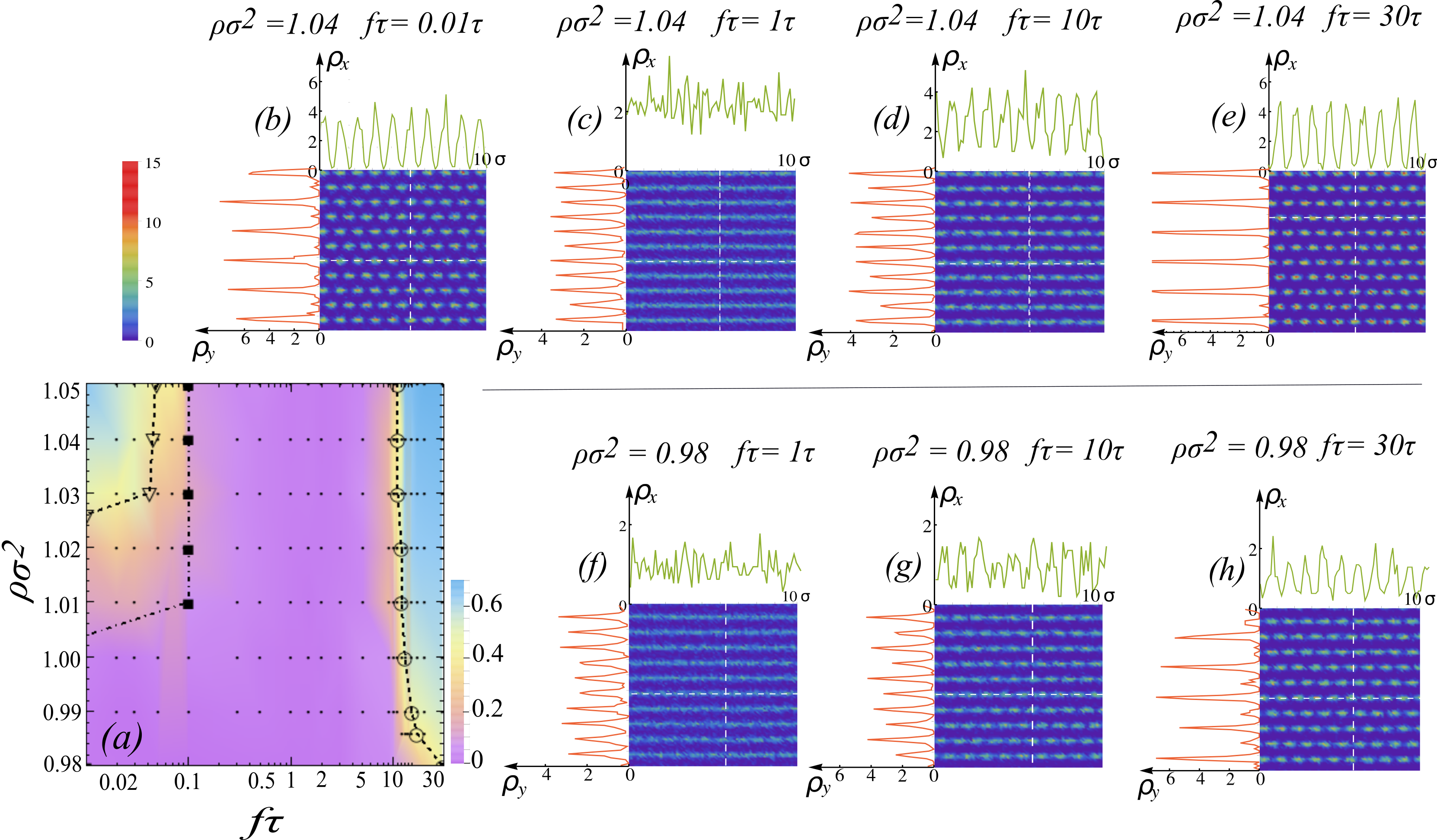
Figure 1: ($a$) Phase diagram in the density- frequency plane. The color code indicates the values of the solid order parameter $\psi_{G}$ of the stochastically ratcheted 2d colloidal suspension at different density and ratcheting frequency. Sky-blue denotes high solid order. The dashed lines through open symbols ($\triangledown$, $\circ$) show the boundaries of instability of the solid phase. The dash-dotted line through $\blacksquare$ indicates the low driving frequency $f_{s}$ below which the system can relax to instantaneous external potential profile. In the opposite limit of high frequencies, the system feels a time- integrated constant confinement analogous to a laser induced freezing and consequently exhibits a high value of the order parameter. In the regime of intermediate frequencies, the long range order is broken due to the particle current. ($b$)-($h$) Plots of time-averaged local density profiles $\rho(x,y)$ over a section of $10\sigma\times 10\sigma$ area, at different densities and frequencies as indicated in the figures. Their cuts $\rho_{y}$ measured along the vertical white dashed lines, and $\rho_{x}$ measured along the horizontal dashed lines are shown in the out-ward projected ordinate and abscissa, respectively.

In Appendix- B we present the model and details of numerical simulations. In Appendix- C we discuss the detailed phase diagram, explaining the properties of the different non-equilibrium phases. The associated variation of driven directed current with driving frequency and density is shown in Sec.​ C.2. In this section we establish the relation of changing particle current to the non-equilibrium phase transitions. This is followed by a detailed analysis of the melting transitions in terms of the order parameters presented in Sec.​ C.3. In the following three subsections, the phase- transitions are further characterized in terms of the distribution functions of order parameters, correlation functions, and formation of topological defects. We finally conclude presenting a discussion and outlook in Appendix- D.

Appendix B Model and Simulation Details

We consider a two dimensional system of a repulsively interacting colloidal suspension of $N$ particles in a volume $A=L_{x}L_{y}$. The mean inter-particle separation in this system $a^{2}=\sqrt{3}\rho/2$ is set by the particle density $\rho=N/A$. We assume that the colloids repel each other via a shifted soft-core potential $U(r)=\epsilon\,[(\sigma/r)^{12}-2^{-12}]$ when the inter-particle separation $r<r_{c}r_{c}=2\sigma$, and $U(r)=0$ otherwise. The units of energy and length scales are set by $\epsilon$, $\sigma$ respectively. The system evolves under an asymmetric ratchet potential $U_{\rm ext}(x,y,t)=V(t)\left[\sin\left(2\pi y/\lambda\right)+\alpha\sin\left(4\pi y/\lambda\right)\right]$, where the time-dependent strength $V(t)$ switches between $\epsilon$ and $0$ stochastically with a rate $f$. The two sinusoidal terms in the above expression of $U_{\rm ext}$ with $\alpha=0.2$ maintains the asymmetric shape of the potential profile. When it assumes a triangular lattice structure, the separation between consecutive lattice planes in the system is $a_{y}=\sqrt{3}a/2$. We have chosen the periodicity of the external potential $\lambda=a_{y}$, commensurate with the mean lattice spacing. In the absence of the external potential, the soft core solid is expected to undergo a two stage solid- hexatic- liquid transition Kosterlitz and Thouless (1973); Halperin and Nelson (1978); Young (1979); Kapfer and Krauth (2015), with the solid melting point at $\rho\sigma^{2}\approx 1.01$. In the presence of a time- independent potential profile with $V(t)=U_{0}$ and $\alpha=0$, the system undergoes RLIM with increase in $U_{0}$ Wei et al. (1998); Frey et al. (1999); Chaudhuri and Sengupta (2006). At $U_{0}=\epsilon$, the laser induced melting point of the soft-core solid is $\rho\sigma^{2}=0.95$ Chaudhuri and Sengupta (2006).

We perform molecular dynamics simulations of the system in the presence of an external ratcheting potential using the standard leap-frog algorithm Frenkel and Smit (2002) with a time-step $\delta t=0.001\,\tau$ where $\tau=\sigma\sqrt{m/\epsilon}$ is the characteristic time scale. We use $m=1$. The temperature of the system is kept constant at $T=1.0\epsilon/k_{B}$ using a Langevin thermostat characterized by an isotropic friction $\gamma=1/\tau$. At each step a trial move is performed to switch $V(t)$ between $0$ and $\epsilon$, and accepted with a probability $f\,\delta t$. In this paper, we present the results for a large system of $N=262144$ particles. We discard simulations over initial $10^{7}$ steps to ensure achievement of steady state, and the analyses are performed collecting data over further $10^{7}$ steps.

Appendix C Results and Discussion

C.1 Phase diagram

In Fig.​​ 1 we present the detailed phase diagram along with local density profiles of the 2D system of mono-dispersed ratcheted colloids. The system displays a solid and a density modulated hexatic phase, controlled by the dimensionless density $\rho\sigma^{2}$ and ratcheting rate $f\tau$. The color codes in Fig.​​ 1($a$) denote the values of mean solid order parameter. The two dashed lines with open symbols signify the two solid melting boundaries at small and high frequencies. The dash-dotted line with filled squares denotes the inverse of relaxation time-scales $f_{s}$ of the system at a given density. For ratcheting rates slower than this time-scale, the solid and hexatic order can equilibrate to the instantaneous external potential and follow its change. The details of the calculation of such relaxation times are discussed in Appendix- E. We characterize the various phases using the structure factor, the pair correlation function, the solid and hexatic order parameters, and their distribution functions. Further details of such characterization are presented in later sections.

As is shown in Fig.​​ 1($a$), the system remains in a QLRO triangular lattice solid phase at the highest frequencies, if the ambient density permits. As the frequency decreases, the solid melts into a hexatic phase, below the dashed line through open circles (Fig.​​ 1). As is shown later, the melting is a continuous transition and happens via a proliferation of topological defects, including the unbinding of dislocation pairs. The molten phase is a hexatic displaying a unimodal distribution of local- hexatic order parameter. This excludes any possibility of phase coexistence, indicating a continuous transition. As the frequency of the drive is decreased further, below the equilibrium relaxation time, the system starts to follow the time variation of the external potential. As a result, the time-averaged properties turn out to be approximately a superposition of the properties of the equilibrium states in the presence ($V(t)=\epsilon$) and absence ($V(t)=0$) of external potential profile. At high densities ($\rho\sigma^{2}\gtrsim 1.026$) the solid phase is stabilized even at low ratcheting frequencies like $f\tau=0.01$. The melting boundary of this solid is shown by the open $\triangledown$ and dashed line.

In Fig.​​ 1($b$)-($h$) we present the time-averaged local density profiles $\rho(x,y)$ at two mean densities $\rho\sigma^{2}=1.04,\,0.98$. We show the results over local cross- sections of area $10\sigma\times 10\sigma$, for better visibility. At $\rho\sigma^{2}=1.04$, the density profile shows triangular lattice structure at $f\tau=0.01$ (Fig.​​ 1($b$) ). At $f\tau=1$ the solid melts into a phase with density modulation along $y$-axis, the direction of ratcheting drive (Fig.​​ 1($c$) ). The melting is quantified later in terms of vanishingly small solid order. At $f\tau=10$, a local triangular lattice- like pattern reappears, albeit the solid order remains small (Fig.​​ 1($d$) ). The system shows a more compact triangular lattice solid at $f\tau=30$ associated with appearance of significant solid order (Fig.​​ 1($e$) ). As is turns out, this order decreases with the system size in a power law manner, identifying a QLRO solid (see Fig.​​ 5). As we show later, the density modulated phases of the system at $f\tau=1$ and $10$ share similar amount of hexatic order (see Fig.​​ 6).

In the top and left axes around the $\rho(x,y)$ plots, we show the linear density profiles $\rho_{x}$ (ordinate) and $\rho_{y}$ (abscissa) measured along the horizontal and vertical dashed white lines indicated in the $\rho(x,y)$ plots. The clean density modulations in $\rho_{x}$ captures the spontaneous emergence of the solid- like order in that direction. Due to the shape of the triangular lattice solid, $\rho_{y}$ shows large followed by tiny peaks along the white line perpendicular to the lattice planes, e.g., in Fig.​​ 1($b$) and ($e$). Note that this feature is not shared by the other local density plots after the solid melts, shown in Fig.​​ 1. The strong density modulation $\rho_{y}$ in the hexatic phase is induced directly by the external potential minima. This phase lacks density modulation in $\rho_{x}$, as is shown in Fig.​​ 1($c$). However, as we shall quantify later, it shows significant hexatic orientation order.

Similar characterization at the lower density $\rho\sigma^{2}=0.98$ are presented in Fig.​​ 1($f$)-($h$). A clear solid- like triangular lattice order is observed at $f\tau=30$ (Fig.​​ 1($h$) ). Fig.​​ 1($g$) shows local weak triangular lattice like pattern that gets smeared within the hexatic phase. As we show later in Sec.-Sec.​ C.3, this phase in Fig.​​ 1($f$) and ($g$) indeed display a vanishingly small solid order, in the presence of a reasonably large hexatic order. The system remains in the molten phase at the intermediate frequency range, between $0.1\leq f\tau\leq 10$. Note that the densities considered here are relatively large with respect to the equilibrium melting point in the absence of external potential. As we demonstrate in the following, the non-equilibrium melting discussed in this section is associated with an increase in directed particle current carried by the system under the flashing ratchet drive.

C.2 Direct particle current out of alternating drive

The inherent asymmetry of the ratchet potential, added with the stochastic switching drives a time- and space- averaged directed particle current in the system,

$$\left\langle j_{y}\right\rangle=\frac{1}{\tau_{m}}\frac{1}{A}\int^{\tau_{m}}\mathrm{d}\mathrm{t}\int^{L_{x}}\mathrm{d}\mathrm{x}\int^{L_{y}}\mathrm{d}\mathrm{y}~{}j_{y}(x,y,t),$$ (1)

where, $\tau_{m}$ is an integral multiple of $1/f$, the mean switching time of the flashing ratchet potential.

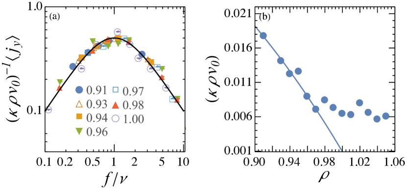
Figure 2: (color online ) (a) Variation of the scaled particle current along the direction of the drive as a function $f/\nu$ for different densities as indicated in the legend. The solid line is plot of the function $(f/\nu)/\left(1+(f/\nu)^{2}\right)$ as given by Eq. 2. (b) Plot of the current amplitude $\rho\kappa v_{0}$ as a function of density. The solid line is a fit to the data using the functional form $\kappa D_{0}\rho^{3/2}(1-\rho/\rho_{c})$ with $\kappa D_{0}$ and $\rho_{c}$ as fitting parameters with values $\kappa D_{0}\approx 0.22$ and $\rho_{c}\sigma^{2}\approx 1.004$.

The competition between the intrinsic relaxation of the system and the external drive leads to a resonance in the mean particle current. At low frequencies the particle current increases linearly with the driving frequency $f$, achieves a maximum around $f=\nu$, and beyond this decays as $f^{-1}$. The behaviour of the current in the whole frequency range can be captured by the simple ansatz Chakraborty and Chaudhuri (2015)

$$\left\langle j_{y}\right\rangle=\kappa\frac{\nu f}{\nu^{2}+f^{2}}\rho v_{0},$$ (2)

where, $\nu$ is the intrinsic relaxation frequency, $v_{0}=\nu\lambda$ intrinsic velocity, and $\kappa$ is a proportionality constant.

In the high density regime, where, the mean-free path of the particles is small, the diffusive time scale $\tau_{D}$ to travel the typical distance $\lambda$ is set by $\tau_{D}=\lambda^{2}/D(\rho)$. Here $D(\rho)$ denotes the density- dependent tagged particle diffusivity, which we assume to decrease linearly with density, $D(\rho)=D_{0}(1-\rho/\rho_{c})$ Lahtinen et al. (2001); Falck and Lahtinen (2004). Here $D_{0}=k_{B}T/\gamma$ is the bare diffusivity. The commensurate external potential ensures that $\lambda^{2}\sim 1/\rho$, and consequently the intrinsic relaxation frequency takes the form $\nu=\rho D(\rho)$. The intrinsic velocity scale is set by $v_{0}=\lambda/\tau_{D}=\rho^{1/2}D(\rho)$. Substituting for $v_{0}$ and $\nu$ in Eq. 2, the density and frequency dependent current takes the form

$$\langle j_{y}\rangle=\frac{fD_{0}^{2}}{D_{0}^{2}\rho^{2}(1-\rho/\rho_{c})^{2}+f^{2}}\rho^{5/2}(1-\rho/\rho_{c})^{2}.$$ (3)

The resonance in the particle current appears at the ratcheting rate $f=\nu=D_{0}\rho(1-\rho/\rho_{c})$ and the density dependent amplitude take the form $\kappa\rho v_{0}=\kappa D_{0}\rho^{3/2}(1-\rho/\rho_{c})$.

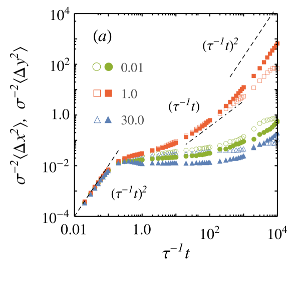
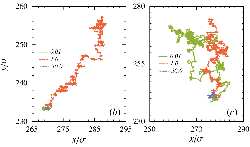
Figure 3: (color online ) Plot of the mean-square displacement at density $\rho\sigma^{2}=1.04$ for frequencies $f\tau=0.01$ (green), $1.0$ (red) and $30.0$ (blue). The displacements in $\langle\Delta x^{2}\rangle$ are shown with open symbols and that in $\langle\Delta y^{2}\rangle$ are represented with filled symbols. Typical trajectories of particles at densities $\rho\sigma^{2}=1.04$ ($b$) and $0.98$ ($c$) are shown for three different frequencies $f\tau=0.01$, $1$ and $30$. At high frequencies the particles get localized, whereas at very low frequencies localization happens only at densities above $\rho_{c}$. In the intermediate frequencies, at both densities the trajectories span a length scale of $\approx 20\,\sigma-30\,\sigma$.

Fig.​​ 2($a$) shows data collapse of particle currents when plotted as $(\kappa\rho v_{0})^{-1}\langle j_{y}\rangle$ against the dimensionless variable $f/\nu$. The current maximizes at the resonance frequency of $f=\nu$. Fig.​​ 2($b$) shows the limit of validity of the approximate form $v_{0}=D_{0}\rho^{1/2}(1-\rho/\rho_{c})$. A comparison of Fig.​​ 1 and Fig.​​ 2$a$ shows the relationship between the structure and dynamics. For example, at the resonance frequency, the system melts in order to carry the largest directed current.

The dynamics at the local scale can be better appreciated by examining trajectories of individual particles. First we consider the system at high density $\rho\sigma^{2}=1.04$. Both the components of the displacement fluctuations in Fig.​​ 3($a$) show an initial ballistic part $\sim t^{2}$ due to the inertial nature of the dynamics. Both in the low and high frequency limits, this crosses over to a sub-diffusive regime ($\sim t^{\nu}$ with $\nu<1$). The test particles show localized motion within cages formed by neighbours (see Fig.​​ 3($b$) ). The intermediate frequency driving at $f\tau=1$ shows a long time diffusive behavior in $x$, $\langle\Delta x^{2}\rangle\sim t$, and almost ballistic motion in $y$, $\langle\Delta y^{2}\rangle\sim t^{\nu}$ with $1<\nu\lesssim 2$ (Fig.​​ 3($a$) ). The corresponding particle trajectories display long excursions in the $y$-direction, as is displayed in Fig.​​ 3($b$).

Fig.​​ 3($c$) shows typical particle trajectories at low densities, $\rho\sigma^{2}=0.98$. They get localized only at the highest driving frequencies $f\tau=30$. At small and intermediate frequencies they show long excursions which are extended mainly in the $y$-direction, the direction of ratchet drive. The localization of trajectories is related to the low directed current carried by the system, and its ordering into a solid phase. Similarly, the extended particle trajectories are related to the melting of the solid and the presence of relatively large directed current.

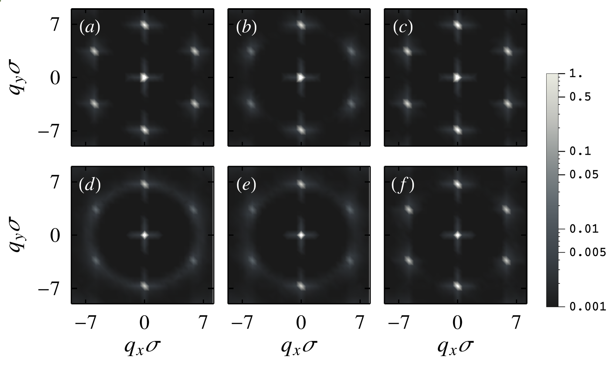
Figure 4: Plots of the static structure factor $\langle\psi_{\bf q}\rangle$ for the densities $\rho\sigma^{2}=1.04$ ($a$-$c$) and $0.98$ (figures $d$-$f$). The three columns correspond to three different frequencies $f\tau=0.01$ ($a$ and $d$), $1.00$ ($b$ and $e$) and $30$ ($c$ and $f$).

C.3 Non-equilibrium melting

For a more quantitative analysis, we turn our attention to the phase diagram Fig.​​ 1($a$) and consider the phase behavior along constant frequency, and constant density lines. The structure factor, $\langle\psi_{\bf q}\rangle=(1/N)\,\langle\rho_{\bf q}\,\rho_{-\bf q}\rangle$ (see Fig.​​ 4) with $\rho_{\bf q}=\sum_{j=1}^{N}e^{-\mathbbm{i}{\bf q}\cdot\bf{r}_{j}}$ and $\rho^{*}_{\bf q}=\rho_{-\bf q}$, can clearly distinguish between a solid, hexatic, liquid and a modulated liquid phase Chaikin and Lubensky (2012). In the solid phase $\langle\psi_{\bf q}\rangle$ shows a characteristic six fold symmetry with peaks at $\mathbf{G}_{1}=(0,\pm 2\pi/a_{y})$ and $\mathbf{G}_{2}=(\pm 2\pi/a,\pm\pi/a_{y})$ reflecting the underlying triangular lattice structure (see Fig.​​ 4($a$),($c$),($f$) ). The six intensity maxima broaden along the constant radius $q=2\pi/a$ circle in a hexatic (Fig.​​ 4($b$),($e$) ). In a simple liquid with spherical symmetry, the broadening extends to overlap forming a characteristic ring structure. On the other hand, in a modulated liquid phase, $\langle\psi_{\bf q}\rangle$ is expected to show two bright spots at $\mathbf{G}_{1}$, in addition to the ring structure characterizing a simple liquid (see Fig.​​ 4($b$),($e$) ). Note that the presence of the external periodic potential in the present context induces an explicit symmetry breaking by imposing density modulations in $y$-direction, ensuring $\langle\psi_{\mathbf{G}_{1}}\rangle>\langle\psi_{\mathbf{G}_{2}}\rangle$. The other four quasi Bragg peaks at $\mathbf{G}_{2}$, e.g., at the highest ratcheting frequencies, identify the appearance of the quasi long ranged positional order (QLRO). We use their arithmatic mean as the measure of solid order parameter $\langle\psi_{\mathbf{G}_{2}}\rangle$.

The QLRO in the solid phase is explicitly demonstrated using the system size dependence of $\langle\psi_{\mathbf{G}_{2}}\rangle$ shown in Fig.​​ 5. The calculations are performed over sub-blocks of sizes $\ell_{x}\times\ell_{y}=\ell^{2}$. Within both the high and low frequency solid regions, $\langle\psi_{\mathbf{G}_{2}}(\ell)\rangle\sim\ell^{-\nu}$ where $\nu<1/3$, the value of the exponent expected at the equilibrium KTHNY (Kosterlitz- Thouless- Halperin- Nelson- Young) melting Kosterlitz and Thouless (1973); Halperin and Nelson (1978); Young (1979). In this case, the value of the exponent $\nu$ depends on the mean density and ratcheting frequency.

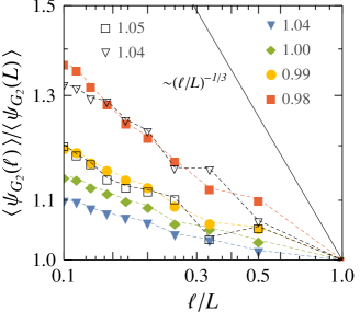
Figure 5: System size dependence of the solid order parameter. The ratio of mean order parameter measured over blocks of size $\ell=(\ell_{x}\times\ell_{y})^{1/2}$ with respect to that measured over the whole system, $\langle\psi_{\mathbf{G}_{2}}(\ell)\rangle/\langle\psi_{\mathbf{G}_{2}}(L)\rangle$ decays with $\ell/L$ with power law $(\ell/L)^{-\nu}$. The data is shown for different densities as indicated in the legend. The solid and open symbols denote results at frequency $f\tau=30$ and $f\tau=0.01$, respectively. The solid black line is a plot of the power-law $(\ell/L)^{-1/3}$ expected at the equilibrium KTHNY melting point.

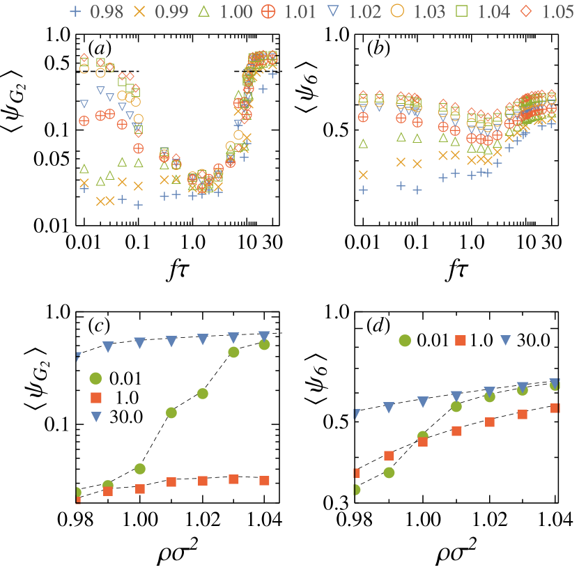
Figure 6: Dependence of the ($a$) solid order parameter $\langle\psi_{\bf{G}_{2}}\rangle$ and ($b$) hexatic order parameter $\langle\psi_{6}\rangle$ as a function of frequency is plotted for different densities as indicated in the legend on the top. The equilibrium melting point $\langle\psi^{m}_{\bf{G}_{2}}\rangle=0.376$ is denoted by the dashed lines in ($a$). The variations of ($c$) $\langle\psi_{\bf{G}_{2}}\rangle$ and ($d$) $\langle\psi_{6}\rangle$ are shown as a function of the mean density for three driving frequencies $f\tau=0.01$, $1$ and $30$ as indicated in the legends.

The phase behaviors are further characterized by following the change in the hexatic bond orientational order $\langle\psi_{6}\rangle=(1/N)\langle|\sum_{i=1}^{N}\ \vec{\psi}^{i}_{6}|^{2}\rangle$, where we define the local hexatic order $\vec{\psi}^{i}_{6}=\sum_{k=1}^{n_{v}}(\ell_{k}/\ell)\exp(\mathbbm{i}6\phi_{ik})$ utilizing the $n_{v}$ Voronoi neighbors of the $i$-th test particle. Here $\phi_{ik}$ is the angle subtended by the bond between the $i$-th particle and its $k$-th Voronoi neighbor. In this definition we used the weighted average over the weight factor $\ell_{k}/\ell$ such that $\ell=\sum_{k=1}^{n_{v}}\ell_{k}$ and $\ell_{k}$ denotes the length of the Voronoi edge corresponding to the $k$-th topological neighbor Mickel et al. (2013).

In Fig.​​ 6($a$) and ($b$) we show the variations of the solid and hexatic orders, $\langle\psi_{\mathbf{G}_{2}}\rangle$ and $\langle\psi_{6}\rangle$, as a function of the ratcheting frequency keeping the density of the system fixed. Fig.​​ 6($c$) and ($d$) show similar plots, but as a function of the density, keeping the driving frequency fixed. Both the order parameters show non-monotonic variation with frequency. The large variation of the solid order parameter $\langle\psi_{\mathbf{G}_{2}}\rangle$ with $f\tau$ signifies melting, followed by a re-entrant solidification. Here we use the value of the solid order parameter at the equilibrium melting point, $\langle\psi^{m}_{\mathbf{G}_{2}}\rangle\approx 0.376$ (Appendix- F), to identify the boundary of solid phase, $\langle\psi_{\mathbf{G}_{2}}\rangle\geq\langle\psi^{m}_{\mathbf{G}_{2}}\rangle$. As we show later, the density-density correlation changes from a power law to an exponential decay across this melting.

As Fig.​​ 6($a$) shows, at all the densities considered the system remains in a solid phase at the highest driving frequencies. With reduction of frequency below $f\tau\approx 10$, the system melts. At densities $\rho\sigma^{2}\gtrsim 1.01$ the system re-solidifies as the frequency is lowered further below $f\tau\approx 0.1$. At intermediate to high frequencies, whether the system remains in a solid or fluid phase is essentially determined by the driving frequency, and not the mean density of the system (see Fig.​​ 6($c$)). Only at the lowest driving frequencies, one finds density dependent solidification. The hexatic order parameter $\langle\psi_{6}\rangle$ shows similar variations, albeit with lesser magnitude (see Fig.​​ 6($b$), ($d$) ). At driving frequencies much larger than the inverse relaxation times, the system responds to only a time-integrated potential profile. The corresponding behavior is similar to that in the presence of a time-independent commensurate potential. For equilibrium melting of the free system, and melting in the presence of a time-independent periodic potential commensurate with the density, see Fig.​​ 12 presented in Appendix- F.

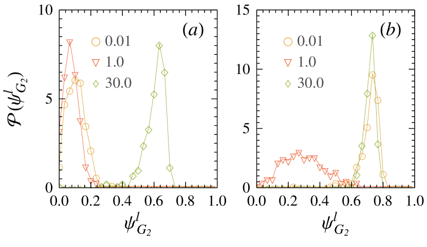
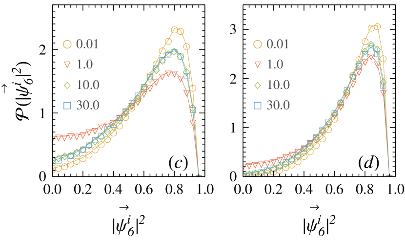
Figure 7: Probability distributions of the local solid and hexatic order parameters $\psi^{l}_{\bf{G}_{2}}$ and $|\vec{\psi}_{6}^{i}|^{2}$. The distribution functions ${\cal P}(\psi^{l}_{\bf{G}_{2}})$ at densities $\rho\sigma^{2}=0.98$ ($a$) and $\rho\sigma^{2}=1.04$ ($b$). The local solid order parameter is determined over subsystems of length $\ell=(\ell_{x}\times\ell_{y})^{1/2}$, where $\ell_{x}/L_{x}=\ell_{y}/L_{y}=1/14$. The distribution functions of local hexatic order ${\cal P}(|\vec{\psi}_{6}^{i}|^{2})$ at $\rho\sigma^{2}=0.98$ ($c$) and $1.04$ ($d$), corresponding to four representative ratcheting frequencies as indicated in the legends.

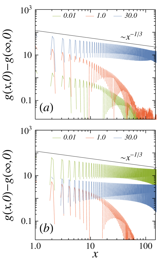
Figure 8: (Color Online) The pair correlation functions $g(x,0)-g(\infty,0)$ calculated at the mean densities $\rho\sigma^{2}=0.98$ ($a$) and $1.04$ ($b$) for the frequencies indicated in the legends.

C.4 Continuous transition: Distribution of order parameters

We probe the order of the phase transitions using the distribution of the local solid and hexatic order parameters. In determining the local solid order, we divided the simulation box into sub-boxes of size $\ell=(\ell_{x}\times\ell_{y})^{1/2}$ with $\ell_{x}/L_{x}=\ell_{y}/L_{y}=1/14$. $\psi^{l}_{\mathbf{G}_{2}}$ is then calculated using the definition of $\psi_{\bf q}$ restricted within these sub-boxes. For the local hexatic order parameter, we calculate $|\rho^{i}_{6}|^{2}$ for all the particles. The distribution functions of these quantities, ${\cal P}(\psi^{l}_{\mathbf{G}_{2}})$ and ${\cal P}(|\rho_{6}|^{2})$ are plotted in Fig.​​ 7. They remain unimodal at all points of the phase diagram. At low densities, $\rho\sigma^{2}=0.98$ in Fig.​​ 7($a$), the maximum of ${\cal P}(\psi^{l}_{\mathbf{G}_{2}})$ appears at an order parameter corresponding to the solid phase only at the highest frequencies. With decreasing frequency the peak shifts towards lower values, signifying melting below $f\tau=10$ and remain low at the lowest frequencies. The unimodal nature of the distribution function, as the peak shifts to lower values, signifies the absence of any metastable state across the transition, a characteristic of continuous transitions. At high densities, e.g., $\rho\sigma^{2}=1.04$ in Fig.​​ 7($b$), corresponding to the re-entrant transition, the peak of the distribution ${\cal P}(\psi^{l}_{\mathbf{G}_{2}})$ shifts from a high to low and back to high values as the ratcheting rate decreases from the highest frequencies. As before, the unimodal nature of the distribution corresponds to a continuous melting transition.

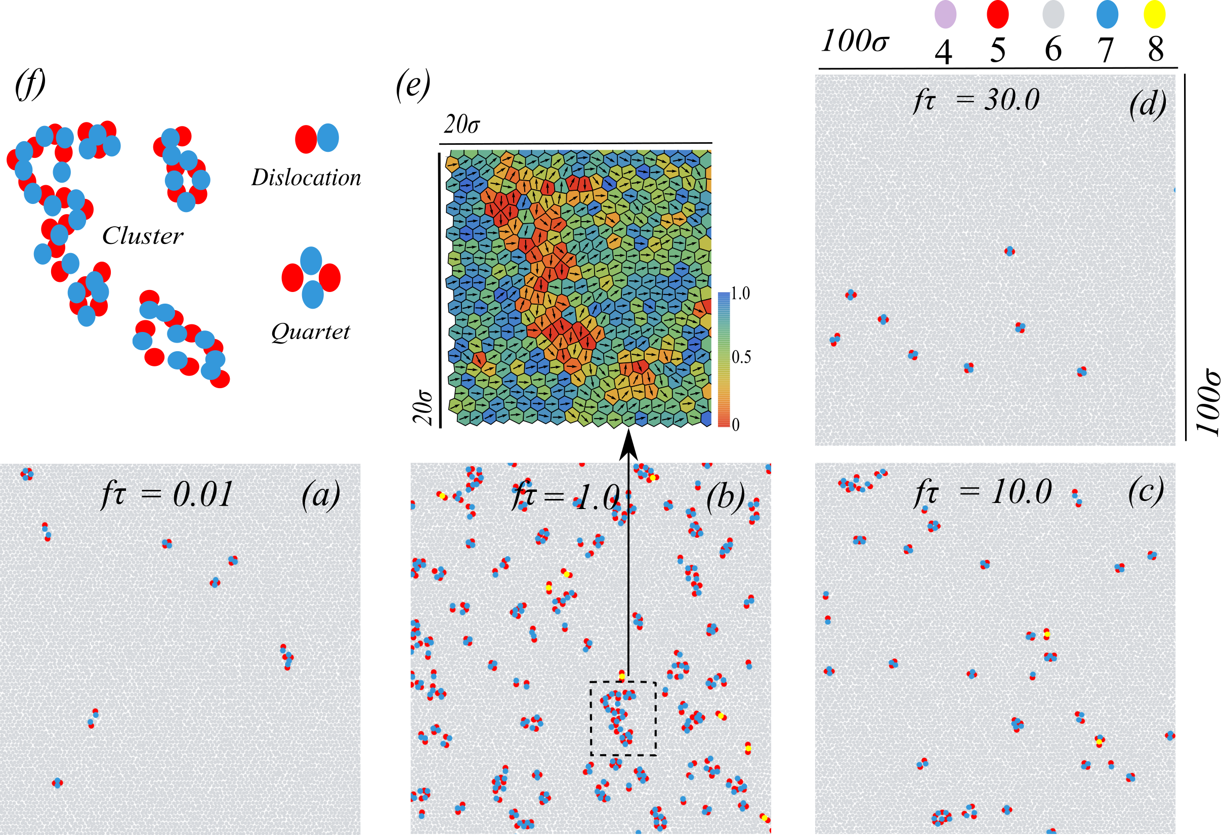
Figure 9: ($a$)-($d$): Configurations of the system in $100\sigma\times 100\sigma$ sub-volumes at a density of $\rho\sigma^{2}=1.04$ for frequencies $f\tau=0.01$ ($a$), $1$ ($b$), $10$ ($c$) and $30$ ($d$). The particles are color coded according to the number of their topological neighbors $n_{v}$, with gray ($n_{v}=6$), blue ($n_{v}=7$), red ($n_{v}=5$), purple ($n_{v}=4$), and yellow ($n_{v}=8$), as shown in the legend on top of ($d$). ($e$) The figure highlights the hexatic order in a region containing a connected string of defects marked by a dashed-box of size $20\sigma\times 20\sigma$ in ($b$). The Voronoi tesselations are shown for each particle within the box and are color coded according to the local value of the hexatic order. The arrows denote the orientation of the local hexatic order $\vec{\psi}_{6}^{i}$. ($f$) Indicate typical examples of defect quartets, dislocations and defect clusters that appear in the system.

The solid melts to a hexatic phase, characterized by the finite hexatic order. However, a further melting of the hexatic is not observed as the frequency is varied. In the density-frequency range bounded between the two dashed lines with open inverted triangles and open circles denoted in Fig.​​ 1 ($a$), the system remains in a hexatic phase. This is corroborated by the distribution of the local hexatic order ${\cal P}(|\rho_{6}|^{2})$ shown in Fig.​​ 7($c$) and ($d$) corresponding to densities $\rho\sigma^{2}=0.98$ and $1.04$, respectively. The uni-modal nature of the distribution with a roughly unchanged peak position and a fat tail persists throughout the frequency range. The peak of the distribution does not shift. However, it is important to note that deep inside the hexatic phase, near $f\tau=1$, a significant fraction of the system displays vanishing hexatic order. This is more prominent at lower densities (see Fig.​​ 7($c$) ). As we show in a later section, local dip in the hexatic order is associated with the formation of grain boundaries.

C.5 Melting of solid: Correlation functions

The pair correlation functions $g(x,y)$ capture the solid melting (see Appendix- G for further details). A density modulation is externally induced in the system along the $y$-direction by the ratcheting drive, breaking the translational symmetry in that direction, explicitly. To study the spontaneous symmetry breaking, here we focus on the $x$-component of the two point correlation functions $g(x,y)$. The component of the correlation $g(x,0)-g(\infty,0)$ along the axis perpendicular to the direction of the ratcheting drive are shown in Fig.​​ 8. This provides a more conclusive evidence to the nature of the phases in different density and frequency regimes. At low densities, as we have shown before, the solid order exists only at the highest frequencies. At such frequencies we find an algebraic decay of the correlation along the $x$ direction, signifying the QLRO (see Fig.​​ 8($a$) ). At intermediate and low frequencies the system melts. This is captured by the exponential decay of the correlation with correlation length $\sim 10\sigma$ (see Fig.​​ 8($a$) ). The scenario changes at higher densities. At high frequency, as before, we again find a solid phase, with the correlation exhibiting algebraic decay corresponding to the QLRO (Fig.​​ 8($b$) ). At high densities, one obtains another solid phase at the low ratcheting frequencies. This also shows algebraic decay of correlations signifying QLRO (see $f\tau=0.01$ graph in Fig.​​ 8($b$) ). The power law $x^{-1/3}$ shown in the figures denote the expected correlation at the onset of the equilibrium KTHNY melting. At the intermediate driving frequencies, $f\tau=1$ in $\rho\sigma^{2}=1.04$ system, the correlation shows exponential decay with a correlation length $\sim 10\,\sigma$, similar to the behavior observed in the low density regime (Fig.​​ 8($b$) ). The change from algebraic to exponential decay is utilized to identify the solid melting points in the phase diagram, as is detailed further in Appendix- G.

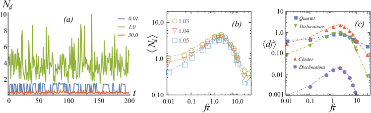
Figure 10: ($a$) Plot of the total defect percentage $N_{d}$ as a function of time for three different driving frequencies as indicated in the legend. The density of the system is $\rho\sigma^{2}=1.04$. At high frequency the system remains in a solid phase, and the defect formation is significantly low ($N_{d}<1\%$). On the other hand, in the opposite limit of low frequency, $f\tau=0.01$, the defect formation follows the swicthing of the driving potential, $N_{d}$ switches between two values. In the intermediate current carrying regime, the formation of the defects is maximized. The defects are further classified by types, e.g., quartets, dislocations, clusters, and disclinations. ($b$) The average defect percentage $\langle N_{d}\rangle$ shows a non-monotonic variation with the ratcheting frequency. We show results at three densities denoted in the legend. ($c$) Variation of the time averaged percentage fraction of the individual defect types, the quartets, dislocations, defect clusters, and disclinations with ratcheting frequency.

C.6 Defect formation

The equilibrium melting of the two- dimensional solid within the continuous KTHNY melting scenario is known to proceed by the unbinding of dislocation pairs into free dislocations. To identify such topological defects, we first obtain the coordination number $n_{v}$ of each particle in the system counting the number of its Voronoi neighbours. In a perfect triangular lattice $n_{v}=6$ for all particles. We follow $n_{v}\neq 6$ particles to identify the $n_{v}$-fold defects. Even within the solid phase, fluctuations of bound quartets of $5-7-5-7$ defects (bound dislocation pairs) keep appearing. They form dislocations by dissociating into separate $5-7$ and $7-5$ non-neighboring pairs. Presence of a finite fraction of particles associated with dislocations characterize the hexatic phase. The system shows dislocation formation as the solid melts. Moreover, we find defect clusters larger than quartets that are either compact or string-like (grain boundary) Qi et al. (2014). All the dominant defect types observed in our simulations are indicated in Fig.​​ 9($f$). Their typical configurations in a sub-volume of size $100\sigma\times 100\sigma$ at $\rho\sigma^{2}=1.04$ and different ratcheting frequencies are shown in Fig.​​ 9($a$)-($d$). In these figures, the colors associated to particles indicate the number of topological neighbors they have, $n_{v}=4\,$(purple), $5\,$(red), $6\,$(green), $7\,$(blue), $8\,$(yellow). Clearly, defect formation is suppressed at both the extremities of the ratcheting frequency. It increases significantly in the intermediate frequency regime associated with solid melting (Fig.​​ 9 ($b$)). The relative fraction of different defect types also vary with the driving frequency. In the highest frequency solids, only bound quartets (bound dislocation pairs) are observed in Fig.​​ 9 $(d)$. As the solid melts with decreasing frequency, dislocations and defect clusters start to appear and eventually dominate over the quartets in the system (Fig.​​ 9 $(b)$ and ($c$) ). The string-like defects remain extended along the $y$-direction, the direction of particle current under ratcheting. Such a connected string of defects is shown in Fig.​​ 9 $(b)$ and has been highlighted in Fig.​​ 9 $(e)$, which shows Voronoi diagram of a region containing the connected string of defects. The color code in each Voronoi cell denotes the amount of hexatic order, and the arrows denote the corresponding hexatic orientations. At the location of the connected clusters of defects, the local hexatic order is low, and shows a hexatic orientation approximately orthogonal to the neighboring defect-free regions. With further lowering of the ratcheting frequency below $f_{s}$, the defect fraction decreases strongly.

This description is quantified by focusing on the time evolution of defect fractions. We first consider the evolution of the total fraction of all the topological defects, the percentage of particles having non-six Voronoi neighbors $N_{d}=(1-n_{6}/N)\times 100$, where $n_{6}$ denotes the total number of particles with $n_{v}=6$ (Fig.​​ 10 $(a)$ ). Clearly, the largest value of $N_{d}$ with the strongest fluctuations appear at the intermediate frequencies. The defect formation gets dramatically suppressed in the solid phase corresponding to the high ratcheting frequencies. At the lowest frequencies ($f\tau=0.01$ in Fig.​​ 10 $(a)$ ), $N_{d}$ remains relatively low and follows the switching of external potential.

The mean value $\langle N_{d}\rangle$ remains less than $4\%$ and varies non-monotonically with $f\tau$ (Fig.​​ 10 $(b)$ ). It shows a maximum at the resonance frequency corresponding to the largest directed current, relating formation of topological defects with carrying capacity of particle current in the system.

Further insight into the structure- dynamics relations can be obtained by following the behavior of different defect fractions separately. For this purpose, the percentage fraction $d_{f}$ of a defect type is defined as $d_{f}=(n_{d}/N)\times 100$, where $n_{d}$ is the total number of $n_{v}\neq 6$ particles that may contribute to either a quartet, a dislocation, a cluster, or a disclination as described above. The time averaged percentage fractions of these topological defects as a function of the driving frequency is shown in Fig.​​ 10 $(c)$. They exhibit a similar non-monotonic behavior as $N_{d}$ and the mean particle current. In the high frequency solid, the dominant defects are the quartets. As the frequency is decreased, the melting of the solid is mediated by the unbinding of these quartets into dislocations. The dislocation fraction becomes larger than that of quartets. More importantly, at the resonance melting, the formation of defect clusters dominate (Fig.​​ 10$(c)$ ). The fraction of disclinations remain relatively insignificant (less than $0.03\%$), about two orders of magnitude smaller than that of the defect clusters. This is consistent with the fact that the hexatic does not melt within these parameter regimes.

Appendix D Discussion

In conclusion, using a large scale simulation involving $262144$ particles, we have presented a detailed study of a ratcheted two-dimensional colloidal suspension, focusing on the structure- dynamics relationship. The mean directed particle current driven by the ratchet exhibits a resonance behavior. Associated with this, the solid melts to hexatic providing a mechanism allowing directed transport. The system exhibits a rich non-equilibrium phase diagram as a function of the driving frequency and mean density. At high densities, we found a re-entrant melting transition as a function of ratcheting frequency. The different phases are characterized by the spatially resolved density profile, the density-density correlation function, the structure factor, the solid and hexatic order parameters, and their distribution functions. The role of the defects in the phase transition has been investigated in detail. The solid- melting is associated with formation of dislocations, but unlike the equilibrium two- dimensional melting, this non-equilibrium melting is dominated by the formation of defect clusters, connected strings of defects that remain oriented largely along the direction of the ratcheting drive. Remarkably, the driven hexatic does not melt to a fluid within the studied range of density and ratcheting drive. Our detailed predictions regarding the variation of particle current and associated phase transitions can be verified using colloidal particles and optical Faucheux et al. (1995) or magnetic ratcheting Tierno (2012) in a suitable laser trapping setup Wei et al. (1998). The impact of changing degree of potential asymmetry on the dynamics and phase behavior remains an interesting future direction of study.

Appendix E Relaxation under external potential

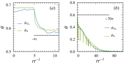
Figure 11: Relaxation dynamics of the solid and hexatic order parameters at $\rho\sigma^{2}=1.04$ ($a$) and $\rho\sigma^{2}=0.98$ ($b$), respectively. The time scales for relaxation are $f_{s}^{-1}\approx 6\,\tau$ ($a$) and $f_{s}^{-1}\approx 70\,\tau$ ($b$).

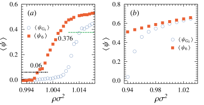
Figure 12: Plot of the solid order parameter $\langle\psi_{\bf{G}_{2}}\rangle$ and the hexatic order parameter $\langle\psi_{6}\rangle$ for the equilibrium phase transition and the laser induced freezing transition. The green dashed line denotes solid melting point $\langle\psi_{{\bf G}_{2}}^{m}\rangle=0.376$, and the black dash-dotted line denotes the hexatic melting point $\langle\psi_{6}\rangle=0.06$.

In this section, we show the results for the relaxation time-scales of the solid and the hexatic order parameters after withdrawing an external potential commensurate with the system density under which the system is initially equilibrated. This time-scale at different densities are determined from separate simulations. The initial equilibration is performed under a time-independent external potential of the form given in Appendix- B with $V(t)=\epsilon$ over $10^{7}$ simulation steps. Thereafter, the external potential is removed and the evolution of the solid and the hexatic order parameters are measured over time.

In Fig.​​ 11 we show the time evolution of these quantities at mean densities $\rho\sigma^{2}=1.04$ (figure $a$) and $0.98$ (figure $b$). At densities higher than the equilibrium melting point $\rho_{m}\sigma^{2}\approx 1.01$, the solid and the hexatic order parameters, $\psi_{\mathbf{G}_{2}}$ and $\psi_{6}$, decay to finite values, indicating order even in the absence of external potential (Fig.​​ 11($a$) ). In contrast, at densities $\rho<\rho_{m}$, the solid and the hexatic order parameters vanish with time (Fig.​​ 11($b$) ). The time-scale of such decay, indicated in Fig.​​ 11, gives the estimate of the relevant relaxation time. If a time-independent external potential switches with a rate slower than this time-scale, the system will have enough time to equilibrate to instantaneous potential profiles. The relaxation frequency $f_{s}$ is inverse of this time-scale, and has been indicated by the dash-dotted line through $\blacksquare$ symbols in the phase diagram Fig.​​ 1.

Appendix F Equilibrium Phase Transition

One way we identified the solid melting in the main text is by choosing an appropriate cutoff value of the solid order parameter $\langle\psi_{\mathbf{G}_{2}}\rangle$. For this, we used the equilibrium melting point in the absence of external potential. To demonstrate this, we perform separate molecular dynamics simulations of particles interacting via the soft-core potential. The temperature of the system is kept fixed at $T=1.0\epsilon/k_{B}$ using a Langevin heat bath. The corresponding variation of $\langle\psi_{\mathbf{G}_{2}}\rangle$ and $\langle\psi_{6}\rangle$ with the mean density is shown in Fig.​​ 12($a$). The order parameters change continuously from low to high values. The solid melting point is separately determined by following the pressure-density curve and the density correlation function as in Ref.33 (data not shown). This melting point is found at density $\rho_{m}\sigma^{2}\approx 1.014$, where the solid order parameter $\langle\psi_{\mathbf{G}_{2}}^{m}\rangle\approx 0.376$. The hexatic order remains significantly large even at lower densities. The melting of hexatic to liquid is identified from the change in correlation of the hexatic order parameter $\langle g_{6}(r)\rangle$, which transforms from an algebraic decay in the hexatic phase to an exponential decay in the liquid. The hexatic- melting is obtained at $\rho\sigma^{2}\approx 0.998$, where $\langle\psi_{6}\rangle\approx 0.06$. In Fig.​​ 12($b$) we show a similar plot for the two order parameters but in the presence of a time- independent potential of the form $U_{ext}(x,y)$ given in Appendix- B with $V(t)=\epsilon$. In the presence of this potential, the hexatic does not melt in the regime of $\rho\sigma^{2}\geq 0.94$. The external potential maintains a significant hexatic order, with a value greater than $\langle\psi_{6}\rangle=0.51$, although the solid order does drop below $0.376$ at $\rho\sigma^{2}\approx 0.96$.

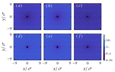
Figure 13: Pair correlation functions in the driven 2D colloidal suspension at densities $\rho\sigma^{2}=1.04$ in the top panels ($a$-$c$) and $\rho\sigma^{2}$=0.98 in the bottom panels ($d$-$f$) corresponding to three different frequencies $f\tau=0.01$ (left column), $f\tau=1$ (middle column) and $f\tau=30$ (right column).

Appendix G Non-equilibrium melting and pair correlation

The two dimensional pair correlation functions $g(x,y)=\langle\rho(x,y)\rho(0,0)\rangle/\langle\rho\rangle^{2}$ at $\rho\sigma^{2}=0.98$ and $\rho\sigma^{2}=1.04$ are shown in Fig.​​ 13 at the three representative frequencies: low ($f\tau=0.01$), intermediate ($f\tau=1$) and high frequency ($f\tau=30$). The figures show the correlations over a length scale of $\pm 9\sigma$. While the clear contrast in Fig.​​ 13($a$), ($c$) and ($f$) demonstrate the triangular lattice symmetry, the local diffused approximately triangular structures in the other $g(x,y)$ figures are characteristic of the hexatic phase.

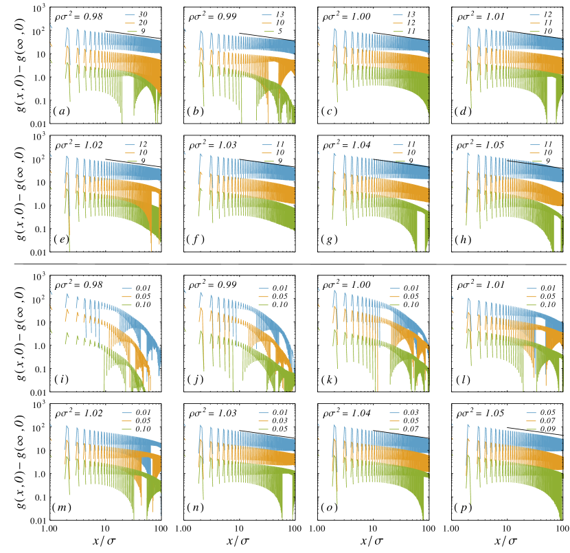
Figure 14: Plots of $g(x,0)-g(\infty,0)$ at different densities $\rho\sigma^{2}$ of the system for frequencies $f\tau$ indicated in the legends. In ($a$)–($h$) we show the data near the high-frequency phase boundary, and in ($i$)–($p$) near the low-frequency phase boundary. The solid black lines denote the power law $x^{-1/3}$ that indicates the expected correlation at the solid melting point within KTHNY thoery Kosterlitz and Thouless (1973); Halperin and Nelson (1978); Young (1979).

The component of the pair correlation function along the minima of the potential $g(x,0)-g(\infty,0)$ changes from a power-law to exponential decay with changing ratcheting frequency, identifying the melting point of a quasi- long ranged ordered solid. In Fig.​​ 14, $(a)$–$(h)$ show the high-frequency melting, while $(i)$–$(p)$ show possible melting at low frequencies.

At $\rho\sigma^{2}\lesssim 1.03$ and low frequencies, the decay of the pair correlation function remains always exponential, identifying an absence of transition. A crossover to an algebraic decay in $g(x,0)-g(x,\infty)$ appears at $\rho\sigma^{2}\gtrsim 1.03$, resulting in solid- hexatic transition points. The phase boundaries displayed in Fig.​​ 1 ($a$) are consistent with the transition points obtained from this analysis.

References

- Julicher et al. (1997) F. Julicher, A. Ajdari and J. Prost, Reviews of Modern Physics, 1997, 69, 1269–1282.
- Astumian and Hänggi (2002) R. D. Astumian and P. Hänggi, Physics Today, 2002, 55, 33.
- Hänggi (2009) P. Hänggi, Reviews of Modern Physics, 2009, 81, 387–442.
- Reimann (2002) P. Reimann, Physics Reports, 2002, 361, 57–265.
- Brouwer (1998) P. Brouwer, Phys. Rev. B, 1998, 58, R10135–R10138.
- Citro et al. (2003) R. Citro, N. Andrei and Q. Niu, Phys. Rev. B, 2003, 68, 165312.
- Jain et al. (2007) K. Jain, R. Marathe, A. Chaudhuri and A. Dhar, Phys. Rev. Lett., 2007, 99, 190601.
- Chaudhuri and Dhar (2011) D. Chaudhuri and A. Dhar, EPL (Europhysics Letters), 2011, 94, 30006.
- Chaudhuri et al. (2015) D. Chaudhuri, A. Raju and A. Dhar, Phys. Rev. E, 2015, 91, 050103.
- Chaudhuri (2015) D. Chaudhuri, J. Phys. Conf. Ser., 2015, 638, 012011.
- Gadsby et al. (2009) D. C. Gadsby, A. Takeuchi, P. Artigas and N. Reyes, Philos. Trans. R. Soc. B Biol. Sci., 2009, 364, 229–238.
- Faucheux et al. (1995) L. Faucheux, L. Bourdieu, P. Kaplan and A. Libchaber, Physical Review Letters, 1995, 74, 1504–1507.
- Lopez et al. (2008) B. Lopez, N. Kuwada, E. Craig, B. Long and H. Linke, Physical Review Letters, 2008, 101, 220601.
- Tierno et al. (2010) P. Tierno, P. Reimann, T. H. Johansen and F. Sagués, Physical Review Letters, 2010, 105, 230602.
- Tierno (2012) P. Tierno, Physical Review Letters, 2012, 109, 198304.
- Rousselet et al. (1994) J. Rousselet, L. Salome, A. Ajdari and J. Prost, Nature, 1994, 370, 446.
- Leibler (1994) S. Leibler, Nature, 1994, 370, 412.
- Marquet et al. (2002) C. Marquet, A. Buguin, L. Talini and P. Silberzan, Physical Review Letters, 2002, 88, 168301.
- Derényi and Vicsek (1995) I. Derényi and T. Vicsek, Physical review letters, 1995, 75, 374.
- Derényi and Ajdari (1996) I. Derényi and A. Ajdari, Physical Review E, 1996, 54, R5–R8.
- Marathe et al. (2008) R. Marathe, K. Jain and A. Dhar, J. Stat. Mech. Theory Exp., 2008, 2008, P11014.
- Savel’ev et al. (2004) S. Savel’ev, F. Marchesoni and F. Nori, Phys. Rev. E, 2004, 70, 061107.
- Pototsky et al. (2010) A. Pototsky, A. J. Archer, M. Bestehorn, D. Merkt, S. Savel’ev and F. Marchesoni, Phys. Rev. E, 2010, 82, 030401.
- Savel’ev et al. (2003) S. Savel’ev, F. Marchesoni and F. Nori, Phys. Rev. Lett., 2003, 91, 010601.
- Chakraborty and Chaudhuri (2015) D. Chakraborty and D. Chaudhuri, Physical Review E - Statistical, Nonlinear, and Soft Matter Physics, 2015, 91, 050301(R).
- Chowdhury et al. (1985) A. Chowdhury, B. J. Ackerson and N. A. Clark, Phys. Rev. Lett., 1985, 55, 833.
- Wei et al. (1998) Q.-H. Wei, C. Bechinger, D. Rudhardt and P. Leiderer, Physical Review Letters, 1998, 81, 2606–2609.
- Frey et al. (1999) E. Frey, D. R. Nelson and L. Radzihovsky, Phys. Rev. Lett., 1999, 83, 2977.
- Chaudhuri and Sengupta (2006) D. Chaudhuri and S. Sengupta, Physical Review E, 2006, 73, 11507.
- Kosterlitz and Thouless (1973) J. M. Kosterlitz and D. J. Thouless, J. Phys. C, 1973, 6, 1181.
- Halperin and Nelson (1978) B. I. Halperin and D. R. Nelson, Phys. Rev. Lett., 1978, 41, 121–124.
- Young (1979) A. P. Young, Phys. Rev. B, 1979, 19, 1855.
- Kapfer and Krauth (2015) S. C. Kapfer and W. Krauth, Physical Review Letters, 2015, 114, 035702–5.
- Frenkel and Smit (2002) D. Frenkel and B. Smit, Understanding molecular simulation: from algorithms to applications, Academic press, NY, 2002.
- Lahtinen et al. (2001) J. Lahtinen, T. Hjelt, T. Ala-Nissila and Z. Chvoj, Physical Review E, 2001, 64, 021204.
- Falck and Lahtinen (2004) E. Falck and J. Lahtinen, The European Physical Journal E, 2004, 13, 267.
- Chaikin and Lubensky (2012) P. M. Chaikin and T. C. Lubensky, Principles of Condensed Matter Physics, Cambridge University Press, Cambridge, 2012.
- Mickel et al. (2013) W. Mickel, S. C. Kapfer, G. E. Schröder-Turk and K. Mecke, J. Chem. Phys., 2013, 138, 044501.
- Qi et al. (2014) W. Qi, A. P. Gantapara and M. Dijkstra, Soft Matter, 2014, 10, 5449–5457.