todostodList of Comments
Distributed Certifiably Correct Pose-Graph Optimization
Abstract
This paper presents the first certifiably correct algorithm for distributed pose-graph optimization (PGO), the backbone of modern collaborative simultaneous localization and mapping (CSLAM) and camera network localization (CNL) systems. Our method is based upon a sparse semidefinite relaxation that we prove provides globally-optimal PGO solutions under moderate measurement noise (matching the guarantees enjoyed by state-of-the-art centralized methods), but is amenable to distributed optimization using the low-rank Riemannian Staircase framework. To implement the Riemannian Staircase in the distributed setting, we develop Riemannian block coordinate descent (RBCD), a novel method for (locally) minimizing a function over a product of Riemannian manifolds. We also propose the first distributed solution verification and saddle escape methods to certify the global optimality of critical points recovered via RBCD, and to descend from suboptimal critical points (if necessary). All components of our approach are inherently decentralized: they require only local communication, provide privacy protection, and are easily parallelizable. Extensive evaluations on synthetic and real-world datasets demonstrate that the proposed method correctly recovers globally optimal solutions under moderate noise, and outperforms alternative distributed techniques in terms of solution precision and convergence speed.
1 Introduction
Collaborative multi-robot missions require consistent collective spatial perception across the entire team. In unknown GPS-denied environments, this is achieved by collaborative simultaneous localization and mapping (CSLAM), in which a team of agents jointly constructs a common model of an environment via exploration. At the heart of CSLAM, robots must solve a pose-graph optimization (PGO) problem (also known as pose synchronization) to estimate their trajectories based on noisy relative inter-robot and intra-robot measurements.
While several prior approaches to CSLAM have appeared in the literature, to date no method has been proposed that is capable of guaranteeing the recovery of an optimal solution in the distributed setting. One general line of prior work [1, 2, 3, 4] proposes to solve CSLAM in a centralized manner. While this approach is straightforward (as it enables the use of off-the-shelf methods for PGO), it imposes several practically-restrictive requirements, including: a central node that is capable of solving the entire team’s SLAM problem, a sufficiently reliable communication channel that connects the central node to the team, and sufficient resources (particularly energy and bandwidth) to regularly relay the team’s (raw or processed) observations to the central node. Moreover, these schemes by construction are unable to protect the spatial privacy of individual robots, and lack robustness due to having a single point of failure. An alternative line of work proposes fully distributed algorithms [5, 6, 7, 8]; however, at present these methods are all based upon applying distributed local optimization methods to the nonconvex PGO problem [5, 9], which renders them vulnerable to convergence to significantly suboptimal solutions [10].
In parallel, over the last several years recent work has developed a novel class of certifiably correct estimation methods that are capable of efficiently recovering provably globally optimal solutions of generally-intractable estimation problems within a restricted (but still practically-relevant) operational regime [11]. In particular, Rosen et al. [12] developed SE-Sync, a certifiably correct algorithm for pose-graph optimization. SE-Sync is based upon a (convex) semidefinite relaxation whose minimizer is guaranteed to provide a globally optimal PGO solution whenever the noise on the available measurements falls below a certain critical threshold; moreover, in the (typical) case that this occurs, it is possible to computationally verify this fact a posteriori, thereby certifying the correctness (optimality) of the recovered estimate. However, SE-Sync is not directly amenable to a decentralized implementation because its semidefinite relaxation generically has dense data matrices, and it solves this relaxation using a second-order optimization scheme, both of which would require an impractical degree of communication among the agents in a distributed setting.
In this paper, we advance the state of the art in CSLAM by proposing the first PGO algorithm that is both fully distributed and certifiably correct. Our method leverages the same semidefinite relaxation strategy that underpins current state-of-the-art (centralized) certifiably correct PGO algorithms [12], but employs novel decentralized optimization and solution verification techniques that enable these relaxations to be solved efficiently in the distributed setting. Specifically, we make the following contributions:
-
•
We prove that a sparse semidefinite relaxation of PGO employed by Briales and Gonzalez-Jimenez [13] enjoys the same exactness guarantees as the one used in SE-Sync [12]: namely, that its minimizers are low-rank and provide exact solutions of the original PGO problem under moderate measurement noise.
-
•
We describe an efficient low-rank optimization scheme to solve this semidefinite relaxation in the distributed setting. Specifically, we employ a distributed Riemannian Staircase approach [14], and propose Riemannian block coordinate descent (RBCD), a novel method for minimizing a function over a product of Riemannian manifolds, to solve the resulting low-rank subproblems in the distributed setting. We prove that RBCD converges to first-order critical points with a global sublinear rate under standard (mild) conditions, and that these are in particular always satisfied for the low-rank PGO subproblems. We also describe Nestorov-accelerated variants of RBCD that significantly improve its convergence speed in practice.
-
•
We propose the first distributed solution verification and saddle escape methods to certify the optimality of low-rank critical points recovered via RBCD, and to descend from suboptimal critical points (if necessary).
-
•
Finally, we describe simple distributed procedures for initializing the distributed Riemannian Staircase optimization, and for rounding the resulting low-rank factor to extract a final PGO estimate.
Each of these algorithmic components has the same communication, computation, and privacy properties enjoyed by current distributed CSLAM methods [5, 8, 7], including:
-
1.
Communication and computational efficiency: Robots need only communicate with their neighbors in the pose graph. To this end, the minimum requirement is that robots form a connected network, so that information can flow between any pair of robots (possibly relayed by intermediate robots). The payload size in each round of communication is only where is the number of inter-robot loop closures. Moreover, local updates in RBCD can be performed efficiently and in parallel, and the solution is produced in an anytime fashion.
-
2.
Spatial privacy protection: Robots are not required to reveal any information about their own observations or their private poses (those poses that are not directly observed by other robots).
Our overall algorithm, Distributed Certifiably Correct Pose-Graph Optimization (DC2-PGO), thus preserves the desirable computational properties of existing state-of-the-art CSLAM methods while enabling the recovery of provably globally optimal solutions in the distributed setting.
The rest of this paper is organized as follows. In the remainder of this section we introduce necessary notations and mathematical preliminaries. In Section 2, we review state-of-the-art centralized and distributed PGO solvers, as well as recent advances in block-coordinate optimization methods. In Section 3, we formally define the distributed PGO problem and present its sparse SDP relaxation. We present a distributed procedure to solve this SDP via the Riemannian Staircase framework. On the theoretical front, we establish formal exactness guarantees for the SDP relaxation. In Section 4, we present our distributed local search method to solve the rank-restricted SDPs using block-coordinate descent. In Section 5, we prove convergence of the proposed local search method and analyze its global convergence rate. In Section 6, we present a distributed solution verification procedure that checks the global optimality of our local solutions, and enables us to escape from suboptimal critical points, if necessary. We discuss distributed initialization and rounding in Section 7. Finally, we conclude with extensive experimental evaluations in Section 8.
Notations and Preliminaries
General Notations
Unless stated otherwise, lowercase and uppercase letters are generally used for vectors and matrices, respectively. We define .
Linear Algebra
and denote the set of symmetric and symmetric positive semidefinite matrices, respectively. are the zero and identity matrix, and represent the vectors of all zeros and all ones, respectively. To ease the burden of notations, we also drop the subscript when the dimension is clear from context. For a matrix , we use to index its -th entry. denotes the Moore-Penrose inverse of . Given a ()-block-structured matrix , refers to its -th block. denotes the orthogonal projection operator onto a given set with respect to the Frobenius norm.
We define several linear operators that will be useful in the rest of this paper. Given a list of square matrices (possibly with different dimensions), assembles them into a block-diagonal matrix:
| (1) |
For an arbitrary square matrix , returns its symmetric part . For a -block-structured matrix , we define the following linear operator that outputs another -block-diagonal matrix as follows,
| (2) |
In addition, for a -block-structured matrix , we define a similar linear operator:
| (3) |
Differential Geometry of Riemannian Manifolds
We refer the reader to [15, 16] for outstanding introductions to Riemannian optimization on matrix submanifolds. In general, we use to denote a smooth matrix submanifold of a real Euclidean space. (or for brevity) denotes the tangent space at . The tangent space is endowed with the standard Riemannian metric induced from the ambient (Euclidean) space, i.e., , and the induced norm is . denotes a retraction operator, with being its restriction to . For a function , we use and to denote the Euclidean and Riemannian gradients of at . For matrix submanifolds, the Riemannian gradient is obtained as the orthogonal projection of the Euclidean gradient onto the associated tangent space:
| (4) |
We call a first-order critical point if . For the second-order geometry, we are primarily concerned with the Riemannian Hessian of a function . For matrix submanifolds, the Riemannian Hessian is a linear mapping on the tangent space which captures the directional derivative of the Riemannian gradient:
| (5) | ||||
Above, the operator denotes the standard directional derivative in the Euclidean space; see [16, Chapter 5].
Matrix submanifolds used in this work
In SLAM, standard matrix submanifolds that frequently appear include the special orthogonal group and the special Euclidean group . We also make use of the Stiefel manifold . The geometry of these manifolds can be found in standard textbooks (e.g. [16]). Given a matrix , if is the singular value decomposition (SVD) of , the projection of onto can be obtained as:
| (6) |
In this work, the following product manifold is also used extensively and we give it a specific name:
| (7) |
In our notation (7), we highlight the constants and and omit the constant , as the latter is essentially fixed (i.e., ). As a product manifold, we can readily characterize the first-order geometry of using those of and . In particular, the tangent space of is given as the Cartesian product of the tangent spaces of individual components. In matrix form, we can write the tangent space as:
| (8) |
The normal space is the orthogonal complement of in the ambient space. It can be shown that the normal space takes the form,
| (9) |
Finally, given a matrix in the ambient space, the orthogonal projection onto the tangent space at (8) is given by:
| (10) | ||||
2 Related Work
2.1 Centralized Pose-Graph Optimization Algorithms
In prior work Rosen et al. [12] developed SE-Sync, a state-of-the-art certifiably correct algorithm for pose-graph optimization. SE-Sync is based upon a (convex) semidefinite relaxation that its authors prove admits a unique, low-rank minimizer providing an exact, globally-optimal solution to the original PGO problem whenever the noise on the available measurements is not too large; moreover, in the (typical) case that exactness obtains, it is possible to verify this fact a posteriori [10], thereby certifying the correctness (optimality) of the recovered estimate. To solve the resulting semidefinite relaxation efficiently, SE-Sync employs the Riemannian Staircase [14], which leverages symmetric low-rank (Burer-Monteiro) factorization [17] to directly search for a symmetric low-rank factor of the SDP solution, and implements this low-dimensional search using the truncated-Newton Riemannian trust-region (RTR) method [18, 16]. This combination of low-rank factorization and fast local search (via truncated-Newton RTR) enables SE-Sync to recover certifiably globally optimal PGO solutions at speeds comparable to (and frequently significantly faster than) standard state-of-the-art local search methods (e.g. Gauss-Newton) [12].
Unfortunately, the specific computational synthesis proposed in SE-Sync does not admit a straightforward distributed implementation. In particular, the semidefinite relaxation underlying SE-Sync is obtained after exploiting the separable structure of PGO to analytically eliminate the translational variables [19]; while this has the advantage of reducing the problem to a lower-dimensional optimization over a compact search space, it also means that the objective matrix of the resulting SDP is generically fully dense. Interpreted in the setting of CSLAM, this reduction has the effect of requiring all poses to be public poses; i.e., every pose must be available to every agent in the team. In addition to violating privacy, implementing this approach in a distributed setting would thus require an intractable degree of communication among the agents.
A similar centralized solver, Cartan-Sync, is proposed by Briales and Gonzalez-Jimenez [13]. The main difference between SE-Sync and Cartan-Sync is that the latter directly relaxes the pose-graph optimization problem without first analytically eliminating the translations; consequently, the resulting relaxation retains the sparsity present in the original PGO problem. However, this alternative SDP relaxation (and consequently Cartan-Sync itself) has not previously been shown to enjoy any exactness guarantees; in particular, its minimizers, and their relation to solutions of PGO, have not previously been characterized. As one of the main contributions of this work, we derive sharp correspondences between minimizers of Cartan-Sync’s relaxation and the original relaxation employed by SE-Sync (Theorem 1); in particular, this correspondence enables us to extend the exactness guarantees of the latter to cover the former, thereby justifying its use as a basis for distributed certifiably correct PGO algorithms.
As a related note, similar SDP relaxations [20, 21, 22, 23] have also been proposed for rotation averaging [24]. This problem arises in a number of important applications such as CNL [25, 26, 27], structure from motion [24], and other domains such as cryo-electron microscopy in structural biology [28]. Mathematically, rotation averaging can be derived as a specialization of PGO obtained by setting the measurement precisions for the translational observations to (practically, ignoring translational observations and states); consequently, the algorithms proposed in this work immediately apply, a fortiori, to distributed rotation averaging.
2.2 Decentralized Pose-Graph Optimization Algorithms
The work by Choudhary et al. [5] is currently the state of the art in distributed PGO solvers and has been recently used by modern decentralized CSLAM systems [29, 30]. Choudhary et al. [5] propose a two-stage approach for finding approximate solutions to PGO. The first stage approximately solves the underlying rotation averaging problem by relaxing the non-convex constraints, solving the resulting (unconstrained) linear least squares problem, and projecting the results back to . The rotation estimates are then used in the second stage to initialize a single Gauss-Newton iteration on the full PGO problem. In both stages, iterative and distributable linear solvers such as Jacobi over-relaxation (JOR) and successive over-relaxation (SOR) [31] are used to solve the normal equations. The experimental evaluations presented in [5] demonstrate that this approach significantly outperforms prior techniques [8, 7]. Nonetheless, the proposed approach is still performing incomplete local search on a non-convex problem, and thus cannot offer any performance guarantees.
In another line of work, Tron et al. [25, 26, 27] propose a multi-stage distributed Riemannian consensus protocol for CNL based on distributed execution of Riemannian gradient descent over where and is the number of cameras (agents). CNL can be seen as a special instance of collaborative PGO where each agent owns a single pose rather than an entire trajectory. In these works, the authors establish convergence to critical points and, under perfect (noiseless) measurements, convergence to globally optimal solutions. See Remark 7 for a specialized form of our algorithm suitable for solving CNL.
Recently, Fan and Murphy [9, 32] proposed a majorization-minimization approach to solve distributed PGO. Each iteration constructs a quadratic upper bound on the cost function, and minimization of this upper bound is carried out in a distributed and parallel fashion. The core benefits of this approach are that it is guaranteed to converge to a first-order critical point of the PGO problem, and that it allows one to incorporate Nesterov’s acceleration technique, which provides significant empirical speedup on typical PGO problems. In this work, we propose a different local search method that performs block-coordinate descent over Riemannian manifolds. Similar to [9, 32], we achieve significant empirical speedup by adapting Nesterov’s accelerated coordinate descent scheme [33] while ensuring global convergence using adaptive restart [34]. However, compared to [32], our method enjoys the computational advantage that each iteration requires only an inexpensive approximate solution of each local subproblem (as opposed to fully solving the local subproblem to a first-order critical point). Lastly, while all distributed methods [5, 25, 26, 27, 9, 32] reviewed thus far are local search techniques, our approach is the first global and certifiably correct distributed PGO algorithm.
2.3 Block-Coordinate Descent Methods
Block-coordinate descent (BCD) methods (also known as Gauss-Seidel-type methods) are classical techniques [31, 35] that have recently regained popularity in large-scale machine learning and numerical optimization [36, 37, 38, 39]. These methods are popular due to their simplicity, cheap iterations, and flexibility in the parallel and distributed settings [31].
BCD is a natural choice for solving PGO in the distributed setting due to the graphical decomposition of the underlying optimization problem. In fact, BCD-type techniques have been applied in the past [40, 41] to solve SLAM. Similarly, in computer vision, variants of the Weiszfeld algorithm have also been used for robust rotation averaging [24, 42]. The abovementioned works, however, use BCD for local search and thus cannot guarantee global optimality. More recently, Eriksson et al. [22] propose a BCD-type algorithm for solving the SDP relaxation of rotation averaging. Their row-by-row (RBR) solver extends the approach of Wen et al. [43] from SDPs with diagonal constraints to block-diagonal constraints. In small problems (with up to rotations), RBR is shown to be comparable or better than the Riemannian Staircase approach [14] in terms of runtime. This approach, however, needs to store and manipulate a dense matrix, which is not scalable to SLAM applications (where is usually one to two orders of magnitude larger than the problems considered in [22]). Furthermore, although in principle RBR can be executed distributedly, it requires each agent to estimate a block-row of the SDP variable, which in the case of rotation averaging corresponds to both public and private rotations of other agents. In contrast, the method proposed in this work does not leak information about robots’ private poses throughout the optimization process.
This work is originally inspired by recent block-coordinate minimization algorithms for solving SDPs with diagonal constraints via the Burer-Monteiro approach [44, 45]. Our recent technical report [46] extends these algorithms and the global convergence rate analysis provided by Erdogdu et al. [45] from the unit sphere (SDPs with diagonal constraints) to the Stiefel manifold (SDPs with block-diagonal constraints). In this work, we further extend our initial results by providing a unified Riemannian BCD algorithm and its global convergence rate analysis.
3 Certifiably Correct Pose-Graph Optimization
In this section, we formally introduce the pose-graph optimization problem, its semidefinite relaxation, and our certifiably correct algorithm for solving these in the distributed setting. Figure 1 summarizes the problems introduced in this section and how they relate to each other.
3.1 Pose-Graph Optimization
Pose-graph optimization (PGO) is the problem of estimating unknown poses from noisy relative measurements. PGO can be modeled as a directed graph (a pose graph) , where and correspond to the sets of unknown poses and relative measurements, respectively. In the rest of this paper, we make the standard assumption that is weakly connected. Let denote the poses that need to be estimated, where each consists of a rotation component and a translation component . Following [12], we assume that for each edge , the corresponding relative measurement from pose to is generated according to:
| (11) | ||||
| (12) |
Above, and denote the true (noiseless) relative rotation and translation, respectively. Under the noise model (11)-(12), it can be shown that a maximum likelihood estimate (MLE) is obtained as a minimizer of the following non-convex optimization problem [12]:
Problem 1 (Pose-Graph Optimization).
| (13a) | ||||
| subject to | (13b) | |||
Collaborative PGO
In collaborative PGO, multiple robots must collaboratively estimate their trajectories in a common reference frame by solving the collective PGO problem distributedly (i.e., without outsourcing data to a single “central” node) using inter-robot collaboration. Each vertex of the collective pose graph represents the pose of a robot at a certain time step. Odometry measurements and intra-robot loop closures connect poses within a single robot’s trajectory. When two robots visit the same place (not necessarily at the same time), they establish inter-robot loop closures that link their respective poses; see [29, 47, 48] and references therein for resource-efficient distributed inter-robot loop closure detection techniques. Figure 2 illustrates simple examples based on CNL and CSLAM. Inter-robot loop closures induce a natural partitioning of collective pose graph nodes into public and private poses, marked in red and black in Figure 2, respectively. Additionally, these inter-agent measurements also create dependencies between the robots. This is captured by the dependency graph shown in Figure 2(c).
Definition 1 (Public and private poses).
Poses that share inter-robot loop closures with poses of other robots are called public poses (or separators [7]). All other poses are private poses.
3.2 SDP Relaxation for PGO
Traditionally, Problem 13 is solved with local search algorithms such as Gauss-Newton. However, depending on the noise level and the quality of initialization, local search algorithms are susceptible to local minima [10]. To address this critical issue, recent works aim to develop certifiably correct PGO solvers. In particular, techniques based on SDP relaxation demonstrate empirical state-of-the-art performance while providing theoretical correctness (global optimality) guarantees under low noise regimes [12, 21, 22].
In this section, we present a semidefinite relaxation of Problem 13 that was first studied in [13]. Let be the block-row matrix obtained by aggregating all rotation and translation variables. Briales and Gonzalez-Jimenez [13] show that the cost function (13a) in Problem 13 can be written in matrix form as , where is a symmetric matrix known as the connection Laplacian formed using all relative measurements. Consider the “lifted” variable . Treating as a -block-structured matrix, we see that several necessary conditions for to satisfy the original constraints (13b) in PGO are,
| (14) | |||
| (15) | |||
| (16) | |||
| (17) |
Dropping the non-convex rank and determinant constraints (15) and (17) yields an SDP relaxation of Problem 13.
Problem 2 (SDP Relaxation for Pose-Graph Optimization [13]).
| (18a) | ||||
| subject to | (18b) | |||
The original SE-Sync algorithm [12] employs a different SDP relaxation for Problem 13, obtained by first exploiting the so-called separable structure of PGO [19] to analytically eliminate the translation variables, and then performing convex relaxation over the resulting rotation-only problem. This approach yields:
Problem 3 (Rotation-only SDP Relaxation for Pose-Graph Optimization [12]).
| (19a) | ||||
| subject to | (19b) | |||
where is obtained by computing a generalized Schur complement of the connection Laplacian (Appendix A).
Remark 1 (Choosing the right SDP for Distributed PGO).
Problem 19 has several advantages over Problem 18, including a compact search space and better numerical conditioning. Nevertheless, unlike in Problem 18, the cost matrix in Problem 19 is generally dense (Appendix A.1). In graphical terms, eliminating the translation variables makes the underlying dependency graph fully connected. This is a major drawback in the distributed setting, since it corresponds to making all of the poses public, thereby substantially increasing the required communication. As we shall see in the following sections, our proposed algorithm relies on and exploits the sparse graphical structure (both intra-robot and inter-robot) of the problem to achieve computational and communication efficiency, and to preserve the privacy of participating robots. Therefore, in this work we seek to solve Problem 18 as a sparse convex relaxation to PGO.
However, in contrast to the SE-Sync relaxation (Problem 19) [12], Problem 18 has not previously been shown to enjoy any exactness guarantees. We now present new results to characterize the connection between the solutions of these problems, thereby extending the guarantee of exactness from Problem 19 to Problem 18.
Theorem 1 indicates that relaxing the additional translational variables when forming Problem 2 does not weaken the relaxation versus the SE-Sync relaxation (Problem 19), nor (crucially) introduce any additional minimizers that do not correspond to PGO solutions. In particular, Theorem 1 and [12, Proposition 2] together imply the following exactness guarantee for Problem 2 under low measurement noise.
Theorem 2 (Exact recovery via Problem 18).
Theorem 2 provides a crucial missing piece for achieving certifiably correct distributed PGO solvers: under low noise (quantified by the deviation in spectral norm of the connection Laplacian from its latent value), one can directly read off a global minimizer to PGO (Problem 13) from the first block row of any solution of the sparse SDP relaxation (Problem 18). As empirically shown in [12, 13], both SDP relaxations are exact in real-world scenarios (see Section 8 for additional empirical evidence).
3.3 Solving the Relaxation: The Distributed Riemannian Staircase
In typical CSLAM scenarios, the dimension of the SDP relaxation can be quite large (e.g. ), and thus it is often impractical to solve Problem 18 using standard (interior-point) methods. In a seminal paper, Burer and Monteiro [17] proposed a more scalable approach to search for low-rank solutions in particular: assume that some solution admits a symmetric low-rank factorization of the form , where and , and then directly search for the low-rank factor . This substitution has the two-fold effect of (i) dramatically reducing the dimension of the search space, and (ii) rendering the positive semidefiniteness constraint on redundant, since for any . In consequence, the rank-restricted version of the original semidefinite program obtained by performing the substitution is actually a lower-dimensional nonlinear program, and so can be processed much more efficiently using standard (local) NLP methods.
For SDPs with block-diagonal constraints, Boumal [14] extends the general approach of Burer and Monteiro [17] by further exploiting the geometric structure of the constraints in the Burer-Monteiro-factored problem. The result is an elegant algorithm known as the Riemannian Staircase, which is used to solve the (large-scale) semidefinite relaxations in SE-Sync [12] and Cartan-Sync [13].
In this work, we show how to implement the Riemannian Staircase approach in a distributed manner, thereby enabling us to solve collaborative PGO. Algorithm 1 presents our distributed Riemannian Staircase algorithm. In each iteration of the Riemannian Staircase, we assume a symmetric rank- factorization where . Writing the blocks of as , the SDP constraints (18b) require that and , for all . Equivalently, the aggregate variable is constrained to live on the product manifold . Imposing the rank- factorization thus transforms the original SDP into the following rank-restricted problem:
Problem 4 (Rank-restricted SDP for Pose-Graph Optimization).
| (21) |
In Section 4, we develop a novel local search algorithm, Riemannian block coordinate descent (RBCD), which we will use to recover first-order critical points of the rank-restricted SDP (Problem 4) in the distributed setting. Inspired by Nesterov’s accelerated coordinate descent [33], we also propose an accelerated variant, RBCD++. In Section 5, we establish global first-order convergence guarantees for both RBCD and RBCD++.
From a first-order critical point , we ultimately wish to recover a solution to the SDP relaxation. To do so, we first lift to the next level of the staircase (i.e., increment rank by one). This can be trivially done by padding with a row of zeros (line 7). The motivations behind this operation will become clear later. By construction, the matrix is feasible in Problem 18. We may verify the global optimality of by checking the (necessary and sufficient) Karush-Kuhn-Tucker (KKT) conditions; for a first-order critical point , this amounts to verifying that a certain dual certificate matrix is positive semidefinite (see line 8). In Section 6, we present the first distributed procedure to carry out this verification. If the dual certificate has a negative eigenvalue, then is not a minimizer of the SDP, and is in fact a saddle point to Problem 21. Fortunately, in this case, the procedure in Section 6 also returns a descent direction, with which we can escape the saddle point (line 14) and restart distributed local search.
Remark 2 (First- vs. second-order optimization in the Riemannian Staircase).
The formulation of the Riemannian Staircase presented in Algorithm 1 differs slightly from its original presentation in [14]: specifically, the latter presupposes access to an algorithm that is capable of computing second-order critical points of Problem 4, whereas the Riemannian block coordinate descent method we employ in line 6 only guarantees convergence to first-order critical points. This has implications for the convergence properties of the overall algorithm: while one can show that the second-order version of the Riemannian Staircase [14, Alg. 1] is guaranteed to terminate at a level when applied to Problem 2 [14, Thm. 3.8],111Strictly speaking, the finite-termination guarantees provided by [14, Thm. 3.8] only hold for the SE-Sync relaxation Problem 19 (cf. [12, Prop. 3]); however, we can extend these guarantees to Problem 2 by exploiting the correspondence between critical points of the low-rank factorizations of Problems 2 and 19 that we establish in Lemma 2 (Appendix A). the weaker (first-order) guarantees provided by RBCD are reflected in a correspondingly weaker set of convergence guarantees for our (first-order) Algorithm 1 provided in the following theorem.
Theorem 3 (Convergence of Algorithm 1).
Let denote the sequence of low-rank factors generated by Algorithm 1 in line 7 using a particular saddle escape procedure described in Appendix C. Then exactly one of the following two cases holds:
-
Algorithm 1 generates an infinite sequence satisfying for all , with
(22) and there exists an infinite subsequence satisfying:
(23)
In a nutshell, Theorem 3 states that Algorithm 1—with a particular version of saddle escape procedure described in Appendix C—either terminates after a finite number of iterations, or generates an infinite sequence of factors that monotonically strictly decrease the objective to the optimal value and that can arbitrarily well-approximate the satisfaction of the KKT condition . We prove this theorem in Appendix C.
We remark that while the convergence guarantees of Theorem 3 are formally weaker than those achievable using a second-order local search method, as a practical matter these differences are inconsequential. In any numerical implementation of the Riemannian Staircase framework, both the second-order criticality of a stationary point (in the second-order version) and the nonnegativity of the minimum eigenvalue (in Algorithm 1) are checked subject to some numerical tolerance ; this accounts for both the finite precision of real-world computers, and the fact that the low-rank factors computed via local search in line 6 are themselves only approximations to critical points, as they are obtained using iterative local optimization methods. In particular, practical implementations of Algorithm 1 (including ours) would replace line 10 with a termination condition of the form “”222This is analogous to the standard stopping criterion for local optimization methods., and (23) guarantees that this condition is satisfied after finitely many iterations for any . As a practical matter, the behavior of Algorithm 1 is far from the pessimistic case described in part of Theorem 3; as we show empirically in Section 8, in real-world applications typically only 1-3 iterations suffice.
3.4 The Complete Algorithm
The distributed Riemannian Staircase (Algorithm 1) is the core computational procedure of our overall algorithm. Nevertheless, to implement a complete distributed method for solving the original PGO problem (Problem 13), we must still specify procedures for (i) initializing the Riemannian Staircase by constructing an initial point , and (ii) rounding the low-rank factor returned by the Riemannian Staircase to extract a feasible solution of the PGO problem. We discuss the details of both distributed initialization and rounding in Section 7. Combining these procedures produces our complete distributed certifiably correct algorithm, DC2-PGO (Algorithm 2).
Since the SDP (Problem 18) is a convex relaxation of PGO, its optimal value is necessarily a lower bound on the global minimum of PGO. Using this fact, we may obtain an upper bound on the suboptimality of the solution returned by DC2-PGO. Specifically, let denote the objective achieved by the final estimate, and let denote the optimal value of Problem 13. Then:
| (24) |
In particular, if , then the SDP relaxation is exact, and . In this case, (24) serves as a certificate of the global optimality of .
4 Distributed Local Search via Riemannian Block-Coordinate Descent
In this section, we introduce a new distributed local search algorithm to identify a first-order critical point of the rank-restricted SDP relaxation (Problem 21), which is needed by the Distributed Riemannian Staircase framework (Algorithm 1, line 6). Our algorithm is applicable to a broad class of smooth optimization problems defined over the Cartesian product of matrix manifolds:
| (25) |
The above problem contains Problem 21 as a special case. Specifically, in distributed PGO, each block exactly corresponds to a robot and corresponds to the search space of this robot’s trajectory. Here, is the number of poses owned by the robot associated to block , and is the total number of robots. For this reason, unless otherwise mentioned, in this section we use the words “block” and “robot” interchangeably.
To solve (25), we leverage the product structure of the underlying manifold and propose a distributed block-coordinate descent algorithm that we call RBCD (Algorithm 3). In each iteration of RBCD, a block is selected to be optimized. Specifically, let be the component of corresponding to the selected block, and let be the (fixed) values of remaining blocks. We update by minimizing the following reduced cost function.
| (26) |
For the rank-restricted SDP (Problem 21) in PGO, the reduced problem for block takes the form,
| (27) |
In the above equation, is the submatrix of formed with the rows and columns that correspond to block (i.e., the trajectory of robot ), and is a constant matrix that depends on the (fixed) public variables of robot ’s neighbors in the pose graph.
Remark 3 (Communication requirements of RBCD).
RBCD is designed such that it can be easily implemented by a network of robots. At each iteration, the team first coordinates to select the next block (robot) to update (Algorithm 3, line 9). Then, to update the selected block (Algorithm 3, line 10), the robot corresponding to this block receives public variables from its neighboring robots in the pose graph. Afterwards, this robot forms and solves its local optimization problem (26), which does not require further communications. Finally, to determine when to terminate RBCD (Algorithm 3, line 8), robots need to collaboratively evaluate their total gradient norm. In practice, checking the termination condition may be done periodically (instead of after every iteration) to save communication resources.
Remark 4 (Block-coordinate minimization on product manifolds).
Prior works (e.g., [44, 45, 46]) have proposed similar block-coordinate minimization (BCM) algorithms to solve low-rank factorizations of SDPs with diagonal or block-diagonal constraints. Our approach generalizes these methods in two major ways. First, while prior methods are explicitly designed for problems over the product of spheres [44, 45] or Stiefel manifolds [46], our algorithm is applicable to the product of any matrix submanifolds. Secondly, prior works [44, 45, 46] require that the cost function to have a certain quadratic form, so that exact minimization of each variable block admits a closed-form solution. In contrast, our algorithm does not seek to perform exact minimization, but instead computes an inexpensive approximate update that achieves a sufficient reduction of the objective (see Section 4.2). This makes our method more general and applicable to a much broader class of smooth cost functions that satisfy a Lipschitz-type condition. We discuss this point in greater detail in Section 5.
The rest of this section is organized to discuss each step of RBCD in detail. We begin in Section 4.1 by discussing block selection rules. These rules determine how blocks are selected at each iteration (Algorithm 3, line 9). In Section 4.2, we propose a general block update rule (Algorithm 3, line 10) based on approximate minimization of trust-region subproblems [18]. In Section 4.3, we further develop an accelerated variant of RBCD based on Nesterov’s celebrated accelerated coordinate-descent algorithm [33], which greatly speeds up convergence near critical points. Finally, in Section 4.4 with show that, using a slight modification of our blocking scheme, we can allow multiple robots to update their coordinates in parallel, thereby speeding up our distributed local search.
4.1 Block Selection Rules
In this section, we describe three mechanisms for selecting which block to update at each iteration of RBCD (Algorithm 3, line 9). We note that similar rules have been proposed in the past; see, e.g., [36, 49, 45].
-
•
Uniform Sampling. The first rule is based on the idea of uniform sampling. At each iteration, each block is selected with equal probability .
-
•
Importance Sampling. In practice, it is often the case that selecting certain blocks leads to significantly better performance compared to others [36]. Therefore, it is natural to assign these blocks higher weights during the sampling process. We refer to this block selection rule as importance sampling. In this work, we set the probability of selecting each block to be proportional to the squared gradient norm, i.e., . Here, denotes the component of the Riemannian gradient of that corresponds to block . Under Lipschitz-type conditions, the squared gradient norm can be used to construct a lower bound on the achieved cost decrement; see Lemma 1.
-
•
Greedy (Gauss-Southwell). We can also modify importance sampling into a deterministic strategy that simply selects the block with the largest squared gradient norm, i.e., . We refer to this strategy as greedy selection or the Gauss-Southwell (GS) rule [36]. Recent works also propose other variants of greedy selection such as Gauss-Southwell-Lipschitz (GSL) and Gauss-Southwell-Quadratic (GSQ) [36]. However, such rules require additional knowledge about the block Lipschitz constants that are hard to obtain in our application. For this reason, we restrict our deterministic selection rule to GS. Despite its simplicity, empirically the GS rule exhibits satisfactory performance; see Section 8.
Remark 5 (Communication requirements of different block selection rules).
In practice, uniform sampling does not incur communication overhead, and can be approximately implemented using synchronized clocks on each robot (to conduct and coordinate BCD rounds) and a common random seed for the pseudorandom number generator (to agree on which robot should update in the next round). In contrast, importance sampling and greedy selection require additional communication overhead at each round, as robots need to evaluate and exchange local gradient norms. In particular, the greedy selection rule can be implemented via flooding gradient norms; see, e.g., the FloodMax algorithm for leader election in general synchronized networks [50, Chapter 4]. This requires robots to have unique IDs and communicate in synchronized rounds. While greedy and importance rules have higher communication overhead than uniform sampling, they also produce more effective iterations and thus converge faster (see Section 8).
4.2 Computing a Block Update
Note that since (26) is in general a nonconvex minimization, computing a block update by exactly solving this problem is intractable. In this section, we describe how to implement a cheaper approach that permits the use of approximate solutions of (26) by requiring only that they produce a sufficient decrease of the objective. In Section 5, we show that under mild conditions, such approximate updates are sufficient to ensure global first-order convergence of RBCD. While there are many options to achieve sufficient descent, in this work we propose to (approximately) solve a single trust-region subproblem using the truncated preconditioned conjugate gradient method [18, 16]. Compared to a full minimization that would solve (26) to first-order critical point, our approach greatly reduces the computational cost. On the other hand, unlike other approximate update methods such as Riemannian gradient descent, our method allows us to leverage (local) second-order information of the reduced cost which leads to more effective updates.
Let be the block that we select to update, and denote the current value of this block (at iteration ) as . We define the pullback of the reduced cost function (26) as follows [16, 51],
| (28) | ||||
Note that the pullback is conveniently defined on the tangent space which itself is a vector space. However, since directly minimizing the pullback is nontrivial, it is approximated with a quadratic model function [16, 51], as defined below.
| (29) |
In (29), is a user-specified mapping on the tangent space. By default, we use the Riemannian Hessian so that the model function is a second-order approximation of the pullback. Then, we compute an update direction on the tangent space by approximately solving the following trust-region subproblem,
| (30) |
To ensure that the obtained update direction yields sufficient descent on the original pullback, we follow standard procedure [18, 16] and evaluate the following ratio that quantifies the agreement between model decrease (predicted reduction) and pullback decrease (actual reduction),
| (31) |
If the above ratio is larger than a constant threshold (default to ), we accept the current update direction and set as the updated value of this block. Otherwise, we reduce the trust-region radius and solve the trust-region subproblem again. Algorithm 4 gives the pseudocode for the entire block update procedure.
In Appendix B, we prove that under mild conditions, we can always find an update direction (the so-called Cauchy step [18, 16]) that satisfies the required termination condition (Algorithm 4, line 12). Furthermore, the returned solution is guaranteed to produce sufficient descent on the cost function, which is crucial to establish global convergence rate of RBCD (Algorithm 3). We discuss the details of convergence analysis in Section 5.
Remark 6 (Solving the trust-region subproblem (30)).
Following [18, 16], we also use the truncated conjugate-gradient (tCG) method to solve the trust-region subproblem (30) inside Algorithm 4. tCG is an efficient “inverse-free” method, i.e., it does not require inverting the Hessian itself, and instead only requires evaluating Hessian-vector products. Furthermore, tCG can be significantly accelerated using a suitable preconditioner. Formally, a preconditioner is a linear, symmetric, and positive-definite operator on the tangent space that approximates the inverse of the Riemannian Hessian. Both SE-Sync [52, 12] and Cartan-Sync [13] have already proposed empirically effective preconditioners for problems similar to (27).333The only difference is the additional linear terms in our cost functions, as a result of anchoring variables owned by other robots. Drawing similar intuitions from these works, we design our preconditioner as,
| (32) |
The small constant ensures that the proposed preconditioner is positive-definite. In practice, we can store and reuse the Cholesky decomposition of for improved numerical efficiency.
Remark 7 (Block update via exact minimization).
Algorithm 4 employs RTR [18] to sufficiently reduce the cost function along a block coordinate. It is worth noting that in some special cases, one can exactly minimize the cost function along any single block coordinate [45, 46]. In the context of PGO, this is the case when every block consists only of a single pose which naturally arises in CNL. We provide a quick sketch in the following. First, note that the reduced problem (27) is an unconstrained convex quadratic over the Euclidean component of (i.e., the so-called lifted translation component). We can thus first eliminate this component analytically by minimizing the reduced cost over the lifted translation vector, thereby further reducing (27) to an optimization problem over . Interestingly, the resulting problem too admits a closed-form solution via the projection operator onto provided in (6) (see also [46, Sec. 2] for a similar approach). Finally, using this solution we can recover the optimal value for the Euclidean component via linear least squares (see, e.g., [19]).
4.3 Accelerated Riemannian Block-Coordinate Descent
In practice, many PGO problems are poorly conditioned. Critically, this means that a generic first-order algorithm can suffer from slow convergence as the iterates approach a first-order critical point. Such slow convergence is also manifested by the typical sublinear convergence rate, e.g., for Riemannian gradient descent as shown in [51]. To address this issue, Fan and Murphy [9, 32] recently developed a majorization-minimization algorithm for PGO. Crucially, their approach can be augmented with a generalized version of Nesterov’s acceleration that significantly speeds up empirical convergence.
Following the same vein of ideas, we show that it is possible to significantly speed up RBCD by adapting the celebrated accelerated coordinate-descent method (ACDM), originally developed by Nesterov [33] to solve smooth convex optimization problems. Compared to the standard randomized coordinate descent method, ACDM enjoys an accelerated convergence rate of . Let denote the dimension (number of coordinates) in the problem. ACDM updates two scalar sequences and three sequences of iterates .
| (33) | ||||
| (34) | ||||
| (35) | ||||
| (36) | ||||
| (37) |
In (36), is the Lipschitz constant of the gradient that corresponds to coordinate . Note that compared to standard references (e.g., [33, 35]), we have slightly changed the presentation of ACDM, so that later it can be extended to our Riemannian setting in a more straightforward manner. Still, it can be readily verified that (33)-(37) are equivalent to the original algorithm.444For example, we can recover (33)-(37) from [35, Algorithm 4], by setting the strong convexity parameter to zero.
In Algorithm 5, we adapt the ACDM iterations to design an accelerated variant of RBCD, which we call RBCD++. We leverage the fact that our manifolds of interest are naturally embedded within some linear space. This allows us to first perform the additions and subtractions as stated in (33)-(37) in the linear ambient space, and subsequently project the result back to the manifold. For our main manifold of interest , the projection operation only requires computing the SVD for each Stiefel component, as shown in (6). Note that the original ACDM method performs a coordinate descent step (36) at each iteration. In RBCD++, we generalize (36) by employing the BlockUpdate procedure (Algorithm 4) to perform a descent step on a block coordinate (Algorithm 5, line 15).
Unlike the convex case, it is unclear how to prove convergence of the above acceleration scheme subject to the non-convex manifold constraints. Fortunately, convergence can be guaranteed by adding adaptive restart [34], which has also been employed in recent works [9, 6]. The underlying idea is to ensure that each RBCD++ update (specifically on the variables) yields a sufficient reduction of the overall cost function. This is quantified by comparing the descent with the squared gradient norm at the selected block (Algorithm 5, line 20), where the constant specifies the minimum amount of descent enforced at each iteration. If this criterion is met, the algorithm simply continues to the next iteration. If not, the algorithm switches to the default block update method (same as RBCD), and restarts the acceleration scheme from scratch. Empirically, we observe that setting close to zero (corresponding to a permissive acceptance criterion) gives the best performance.
Remark 8 (Adaptive vs. fixed restart schemes).
Our adaptive restart scheme requires aggregating information from all robots to evaluate the cost function and gradient norm (Algorithm 5, line 20). This step may become the communication bottleneck of the whole algorithm. While in theory we need adaptive restart to guarantee convergence (see Section 5), a practical remedy is to employ a fixed restart scheme [34] whereby we simply restart acceleration (Algorithm 5, lines 21-26) periodically in fixed intervals. Our empirical results in Section 8 show that the fixed restart scheme also achieves significant acceleration, although is inferior to adaptive restart scheme.
Remark 9 (Communication requirements of RBCD++).
With fixed restart, the communication pattern of RBCD++ is identical to RBCD. In particular, with synchronized clocks, robots can update the scalars and (line 10) locally in parallel. Similarly, the “ update” (line 12) and “ update” steps (line 18) do not require communication, since both only involve local linear combinations and projections to manifold. The main communication happens before the “ update” (line 15), where each robot communicates the public components of their variables with neighbors in the global pose graph. Finally, if adaptive restart is used, robots need to communicate and aggregate global cost and gradient norms to evaluate the restart condition (line 20).
4.4 Parallel Riemannian Block-Coordinate Descent
Thus far in each round of RBCD and RBCD++ (Algorithms 3 and 5), exactly one robot performs BlockUpdate (Algorithm 4). However, after a slight modification of our blocking scheme, multiple robots may update their variables in parallel as long as they are not neighbours in the dependency graph (i.e., do not share an inter-robot loop closure; see Figure 2(c)). This is achieved by leveraging the natural graphical decomposition of objectives in Problem 21 (inherited from Problem 13). Updating variables in parallel can significantly speed up the local search.
Gauss-Seidel-type updates can be executed in parallel using a classical technique known as red-black coloring (or, more generally, multicoloring schemes) [31]. We apply this technique to PGO (Figure 3):
-
1.
First, we find a coloring for the set of robots such that adjacent robots in the dependency graph have different colors (Figure 3(a)). Although finding a vertex coloring with the smallest number of colors is NP-hard, simple greedy approximation algorithms can produce a -coloring, where is the maximum degree of the dependency graph; see [53, 54] and the references therein for distributed algorithms. Note that is often bounded by a small constant due to the sparsity of the CSLAM dependency graph.
-
2.
In each iteration, we select a color (instead of a single robot) by adapting the block selection rules presented in Section 4.1. The robots that have the selected color then update their variables in parallel.
Implementing the (generalized) importance sampling and greedy rules (Section 4.1) with coloring requires additional coordination between the robots. In particular, the greedy rule requires computing the sum of squared gradient norms for each color at the beginning of each iteration. Similar to Section 4.1, a naïve approach would be to flood the network with the current squared gradient norms such that after a sufficient number of rounds (specifically, the diameter of the dependency graph), every robot aggregates all squared gradient norm information for every color. Robots can then independently compute the sum of squared gradient norms for every color and update their block only if their color has the largest gradient norm among all colors. We conclude this part by noting that it is also possible to allow all robots to update their private variables in all iterations (irrespective of the selected color) because private variables are separated from each other by public variables.
5 Convergence Analysis for Riemannian Block-Coordinate Descent
In this section, we formally establish first-order convergence guarantees for RBCD (Algorithm 3) and its accelerated variant RBCD++ (Algorithm 5), for generic optimization problems of the form (25) defined on the Cartesian product of smooth matrix submanifolds. Then, at the end of this section, we remark on how our general convergence guarantees apply when solving the rank-restricted SDPs of PGO (Remark 10), with detailed proofs and discussions in Appendix B.4. Our global convergence proofs extend the recent work of Boumal et al. [51]. Similar to [51], we begin by listing and discussing several mild technical assumptions.
Assumption 1 (Lipschitz-type gradient for pullbacks).
In the optimization problem (25), consider the reduced cost and its pullback for an arbitrary block . There exists a constant such that at any iterate generated by a specified algorithm, the following inequality holds for all ,
| (38) |
In [51], Boumal et al. use (38) as a convenient generalization of the classical property of Lipschitz continuous gradient. With this property, the authors show that it is straightforward to establish global first-order convergence guarantees, e.g., for the well-known Riemannian gradient descent algorithm. Furthermore, it is shown that (38) holds under mild conditions in practice, e.g., whenever the cost function has Lipschitz continuous gradients in the ambient Euclidean space and the underlying submanifold is compact [51, Lemma 2.7]. In Appendix B.4, we will generalize this result to show that Assumption 38 holds when running RBCD and RBCD++ in the context of PGO.
Assumption 2 (Global radial linearity of ).
Assumption 3 (Boundedness of ).
Assumption 4 (Lower bound on initial trust-region radius).
Assumptions 39-42 concern the execution of BlockUpdate (Algorithm 4), and are once again fairly lax in practice. In particular, the simplest choice of that satisfies radial linearity (39) and boundedness (40) is the identity mapping. In our PGO application, we use the Riemannian Hessian to leverage local second-order information for faster convergence. In this case, is still radially linear, and in Appendix B.4 we show that is also bounded along the sequence of iterates generated by RBCD or RBCD++. Finally, Assumption 42 can be easily satisfied by using a sufficiently large initial trust-region radius. We are now ready to establish an important theoretical result, which states that each block update (Algorithm 4) yields sufficient decrease on the corresponding reduced cost function.
Lemma 1 (Sufficient descent property of Algorithm 4).
Lemma 1 states that after each iteration of RBCD, we are guaranteed to decrease the corresponding reduced cost function. Furthermore, the amount of reduction is lower bounded by some constant times the squared gradient norm at the selected block. Thus, if we execute RBCD for long enough, intuitively we should expect the iterates to converge to a solution where the gradient norm is zero (i.e., a first-order critical point). The following theorem formalizes this result.
Theorem 4 (Global convergence rate of RBCD).
Let denote the global minimum of the optimization problem (25). Denote the iterates of RBCD (Algorithm 3) as , and the corresponding block selected at each iteration as . Under Assumptions 38-42, RBCD with uniform sampling or importance sampling have the following guarantees,
| (44) |
In addition, RBCD with greedy selection yields the following deterministic guarantee,
| (45) |
Theorem 45 establishes a global sublinear convergence rate for RBCD.555 We note that in our current analysis, uniform sampling and importance sampling share the same convergence rate estimate. In practice, however, it is usually the case that importance sampling yields much faster empirical convergence (see Section 8). This result suggests that it is possible to further improve the convergence guarantees for importance sampling. We leave this for future work. Specifically, as the number of iterations increases, the squared gradient norm decreases at the rate of . Using the same proof technique, we can establish a similar convergence guarantee for the accelerated version RBCD++.
Theorem 5 (Global convergence rate of RBCD++).
Let denote the global minimum of the optimization problem (25). Denote the iterates of RBCD++ (Algorithm 5) as , and the corresponding block selected at each iteration as . Define the constant,
| (46) |
Under Assumptions 38-42, RBCD++ with uniform sampling or importance sampling have the following guarantees,
| (47) |
In addition, RBCD++ with greedy selection yields the following deterministic guarantee,
| (48) |
Remark 10 (Convergence on Problem 4).
So far, we have shown that under mild conditions, RBCD and RBCD++ are guaranteed to converge when solving general optimization problems defined on the Cartesian product of smooth matrix submanifolds. Recall that in the specific application of PGO, we are using RBCD and RBCD++ to solve a sequence of rank-restricted semidefinite relaxations (Problem 4). In Appendix B.4, we show that Assumptions 38-42 are satisfied in this case, and hence RBCD and RBCD++ retain their respective convergence guarantees. In particular, we show that although Assumption 38 (Lipschitz-type gradient) and Assumption 40 (bounded Hessian) do not hold globally (due to the non-compact translation search space), they still hold within the sublevel set of the cost function determined by the initial iterate . Since RBCD and RBCD++ are inherently descent methods, it suffice to restrict our attention to this initial sublevel set as future iterates will not leave this set. The reader is referred to Appendix B.4 for more details.
Remark 11 (Convergence under parallel executions).
With the parallel iterations described in Section 4.4, we can further improve the global convergence rates of RBCD and RBCD++ in Theorems 45 and 48. For example, the constant that appears in the rate estimates of uniform sampling and importance sampling (44) can be replaced by the number of aggregate blocks (colors) in the dependency graph. Recall that in practice, this is typically bounded by a small constant, e.g., the maximum degree in the sparse robot-level dependency graph (see Section 4.4).
6 Distributed Verification
In this section we address the problem of solution verification [10] in the distributed setting. Concretely, we propose distributed solution verification and saddle escape algorithms to certify the optimality of a first-order critical point of the rank-restricted relaxation (21) as a global minimizer of problem (18), and for escaping from suboptimal stationary points after ascending to the next level of the Riemannian Staircase (Algorithm 1). To the best of our knowledge, these are the first distributed solution verification algorithms to appear in the literature.
Our approach is based upon the following simple theorem of the alternative, which is a specialization of [55, Theorem 4] to problems (18) and (21):
Theorem 6 (Solution verification and saddle escape).
Let be a first-order critical point of the rank-restricted semidefinite relaxation (21), and define:
| (49a) | |||
| (49b) |
Then exactly one of the following two cases holds:
-
and is a global minimizer of (18).
-
There exists such that , and in that case:
(50) is a first-order critical point of (21) attaining the same objective value as , and
(51) is a second-order direction of descent from . In particular, taking to be the eigenvector corresponding to the smallest eigenvalue of satisfies the above conditions.
Remark 12 (Interpretation of Theorem 6).
Let us provide a bit of intuition for what Theorem 6 conveys. Part (a) is simply the standard (necessary and sufficient) conditions for to be the solution of the (convex) semidefinite program (18) [56]. In the event that these conditions are not satisfied (and therefore is not optimal in (18)), there must exist a direction of descent from that is not captured in the low-rank factorization (21), at least to first order (since is stationary). This could be because is a saddle point of the nonconvex problem (21) (in which case there may exist a second-order direction of descent from ), or because the descent direction is towards a set of higher-rank matrices than the rank- factorization used in (21) is able to capture. Part (b) of Theorem 6 provides an approach that enables us to address both of these potential obstacles simultaneously, by using a negative eigenvector of the certificate matrix to construct a second-order direction of descent from , the lifting of to the next (higher-rank) “step” of the Riemannian Staircase. Geometrically, this construction is based upon the (easily verified) fact that is the Hessian of the Lagrangian of the extrinsic (constrained) form of (21), and therefore , so that is indeed a direction of second-order descent from the lifted stationary point [55, 57, 58].
In summary, Theorem 6 enables us to determine whether a first-order critical point of (21) corresponds to a minimizer of (18), and to descend from if necessary, by computing the minimum eigenpair of the certificate matrix defined in (49). In the original SE-Sync algorithm, the corresponding minimum-eigenvalue computation is performed by means of spectrally-shifted Lanczos iterations [12, 52]; while this works well for the centralized SE-Sync method, adopting the Lanczos algorithm in the distributed setting would require an excessive degree of communication among the agents. Therefore, in the next subsection, we investigate alternative strategies for computing the minimum eigenpair that are more amenable to a distributed implementation.
6.1 Distributed Minimum-eigenvalue Computation
In this subsection we describe an efficient distributed algorithm for computing the minimum eigenpair of the certificate matrix required in Theorem 6. We begin with a brief review of eigenvalue methods.
In general, the Lanczos procedure is the preferred technique for computing a small number of extremal (maximal or minimal) eigenpairs of a symmetric matrix [59, Chp. 9]. In brief, this method proceeds by approximating using its orthogonal projection onto the Krylov subspace:
| (52) |
where is an initial vector and is a matrix whose columns (called Lanczos vectors) provide an orthonormal basis for . Eigenvalues of the (low-dimensional) approximation , called Ritz values, may then be taken as approximations for eigenvalues of . The -dimensional Krylov subspace in (52) is iteratively expanded as the algorithm runs (by computing additional matrix-vector products), thereby providing increasingly better approximations of ’s extremal eigenvalues (in accordance with the Courant-Fischer variational characterization of eigenvalues [59, Thm. 8.1.2]). The Lanczos procedure thus provides an efficient means of estimating a subset of ’s spectrum (particularly its extremal eigenvalues) to high accuracy at the cost of only a relatively small number (compared to ’s dimension ) of matrix-vector products, especially if the initial vector lies close to an eigenvector of . In particular, if and is the eigenvector associated to , it is well-known that the error in the eigenvector estimate from the maximal Ritz pair decays asymptotically according to [60, eq. (2.15)]:
| (53) |
where
| (54a) | |||
| (54b) |
However, while the Lanczos procedure is the method of choice for computing a few extremal eigenpairs in the centralized setting, it is unfortunately not well-suited to distributed computations when inter-node communication is a bottleneck. This is because the Lanczos vectors must be periodically re-orthonormalized in order to preserve the accuracy of the estimated eigenpairs . While several strategies have been proposed for performing this reorthonormalization, all of them essentially involve computing a QR decomposition of (possibly a subset of columns from) (see [59, Sec. 9.2] and the references therein). Constructing this decomposition in the distributed setting would require frequent synchronized all-to-all message passing, which is impractical when inter-node communication is expensive or unreliable.
We are therefore interested in exploring alternatives to the Lanczos method that require less coordination in the distributed setting. Many commonly-used eigenvalue methods can be viewed as attempts to simplify the “gold-standard” Lanczos procedure, achieving a reduction in storage and per-iteration computation at the cost of a slower convergence rate. An extreme example of this is the well-known power method [59, Sec. 8.2], which can be viewed as a simplification that retains only the final generator of the Krylov subspace in (52) at each iteration. This leads to a very simple iteration scheme, requiring only matrix-vector products:666Note that while the power method iteration is commonly written in the normalized form , normalization is only actually required to compute the Ritz value associated with .
| (55) |
Note that with , the matrix-vector product in (55) can be computed using the same inter-agent communication pattern already employed in each iteration of the RBCD method developed in Section 4, and so is well-suited to a distributed implementation. However, the power method’s simplicity comes at the expense of a reduced convergence rate. In particular, if and are the two largest-magnitude eigenvalues of (with ), then the vector in the Ritz estimate computed via the power method converges to the dominant eigenvector of according to [59, Thm. 8.2.1]:
| (56) |
Let us compare the rates (53) and (56) for the case in which the eigengap is small relative to the diameter of the spectrum of (which is of the same order order as and for the Lanczos and power methods, respectively); intuitively, this is the regime in which the problem is hard, since it is difficult to distinguish and (and consequently their associated eigenspaces). In particular, let us compute the number of iterations required to reduce the angular error in the dominant Ritz vector by the factor . For the Lanczos method, using (53) and (54) and assuming , we estimate:
| (57) |
Similarly, using (56), the analogous estimate for the power method is:
| (58) |
In our target application (certifying the optimality of a first order-critical point ), the minimum eigenvalue we must compute will always belong to a tight cluster whenever is a global minimizer,777This is an immediate consequence of the (extrinsic) first-order criticality condition for (21), which requires , i.e., that each row of be an eigenvector of with eigenvalue [52, Sec. III-C]. so the power method’s dependence upon the eigengap translates to a substantial reduction in performance versus the Lanczos method’s rate.
In light of these considerations, we propose to adopt the recently-developed accelerated power method [61] as our distributed eigenvalue algorithm of choice. In brief, this method modifies the standard power iteration (55) by adding a Polyak momentum term, producing the iteration:
| (59) |
where is a fixed constant. We note that because is constant, the iteration (59) has the same communication pattern as the standard power method (55), and so is well-suited to implementation in the distributed setting. Furthermore, despite the simplicity of the modification (59) versus (55), the addition of momentum actually allows the accelerated power method to match the dependence of the Lanczos method on the dominant eigengap for a well-chosen parameter . More precisely, we have the following result:
Theorem 7 (Theorem 8 of [61]).
Let with eigenvalues , and be the eigenvector associated with the maximum eigenvalue . Given satifying and an initial Ritz vector , after accelerated power iterations (59) the angular error in the Ritz vector satisfies:
| (60) |
Remark 13 (Selection of ).
While the hypotheses of Theorem 7 require that , note that lower bounds on (which provide admissible values of ) are easy to obtain; indeed, the Courant-Fischer theorem [59, Thm. 8.1.2] implies that for any unit vector . We also observe that the bound on the right-hand side of (60) is an increasing function of for and a decreasing function for , with
| (61) |
consequently, the optimal rate is achieved in the limit .
Combining the power and accelerated power methods with the spectral shifting strategy proposed in [52, Sec. III-C] produces our distributed minimum-eigenvalue method (Algorithm 6). In brief, the main idea is to construct a spectrally-shifted version of the certificate matrix such that (i) a maximum eigenvector of coincides with a minimum eigenvector of , and (ii) , so that we can recover the maximum eigenpair of using accelerated power iterations (59). Algorithm 6 accomplishes this by first applying the (basic) power method (55) to estimate the dominant eigenpair of in line 3 (which does not require ), and then applying the accelerated power method to compute the maximum eigenpair ( of in line 7. Note that while the minimum eigenvalue of belongs to a tight cluster whenever is optimal for (21) (necessitating our use of accelerated power iterations in line 7), the dominant eigenvalue of is typically well-separated, and therefore can be computed to high precision using only a small number of power iterations in line 3.
Remark 14 (Communication requirements of Algorithm 6).
The bulk of the work in Algorithm 6 lies in updating the eigenvector estimate via the matrix-vector products (55) and (59). In the distributed regime, these can be implemented by having each robot estimate the block of the eigenvector that corresponds to its own poses. The communication pattern of this process is determined by the sparsity structure of the underlying matrix, which for our application are the dual certificate and its spectrally-shifted version . Fortunately, both and inherit the sparsity of the connection Laplacian . This means that at each iteration of (55) or (59), each robot only needs to communicate with its neighbors in the global pose graph. Therefore, Algorithm 6 provides an efficient way (in terms of both computation and communication) to compute a minimum eigenpair of in the distributed setting.
6.2 Descent from Suboptimal Critical Points
In this subsection we describe a simple procedure for descending from a first-order critical point of Problem 4 and restarting local optimization in the event that is not a minimizer of Problem 2 (as determined by , where is the minimum eigenpair of the certificate matrix in Theorem 6).
In this setting, Theorem 6(b) shows how to use the minimum eigenvector of to construct a second-order direction of descent from the lifting of to the next level of the Riemannian Staircase. Therefore, we can descend from by performing a simple backtracking line-search along ; we summarize this procedure as Algorithm 7. Note that since and by Theorem 6(b), letting , there exists a stepsize such that and for all , and therefore the loop in line 7 is guaranteed to terminate after finitely many iterations. Algorithm 7 is thus well-defined. Moreover, since decreases at an exponential rate (line 8), in practice only a handful of iterations are typically required to identify an acceptable stepsize. Therefore, even though Algorithm 7 requires coordination among all of the agents (to evaluate the objective and gradient norm each trial point , and to distribute the trial stepsize ), it requires a sufficiently small number of (very lightweight) globally-synchronized messages to remain tractable in the distributed setting. Finally, since the point returned by Algorithm 7 has nonzero gradient, it provides a nonstationary initialization for local search at the next level of the Riemannian Staircase (Algorithm 1), thereby enabling us to continue the search for a low-rank factor in Problem 21 corresponding to a global minimizer of the SDP relaxation Problem 2.
7 Distributed Initialization and Rounding
7.1 Distributed Initialization
A distinguishing feature of our approach versus prior distributed PGO methods is that it enables the direct computation of globally optimal solutions of the PGO problem (13) via (convex) semidefinite programming, and therefore does not depend upon a high-quality initialization in order to recover a good solution. Nevertheless, it can still benefit (in terms of reduced computation time) from being supplied with a high-quality initial estimate whenever one is available.
Arguably the simplest method of constructing such an initial estimate is spanning tree initialization [62]. As the name suggests, we compute the initial pose estimates by propagating the noisy pairwise measurements along an arbitrary spanning tree of the global pose graph. In the distributed scenario, this technique incurs minimal computation and communication costs, as robots only need to exchange few public poses with their neighbors.
While efficient, the spanning tree initialization is heavily influenced by the noise of selected edges in the pose graph. A more resilient but also more heavyweight method is chordal initialization, originally developed to initialize rotation synchronization [63, 64]. With this technique, one first relaxes rotation synchronization into a linear least squares problem, and subsequently projects the solution back to the rotation group. For distributed computation, Choudhary et al. [5] propose to solve the resulting linear least squares problem via distributed iterative techniques such as the Jacobi and Gauss-Seidel methods [31]. One detail to note is that in [5], the translation estimates are not explicitly initialized but are instead directly optimized during a single distributed Gauss-Newton iteration. However, we find that this approach leads to poor convergence for [5] on some real-world datasets. To resolve this, in this work we also explicitly initialize the translations by fixing the rotation initialization and using distributed Gauss-Seidel to solve the reduced linear least squares over translations. On the other hand, to prevent significant communication usage in the initialization stage, we limit the number of Gauss-Seidel iterations to 50 for both rotation and translation initialization.
Lastly, we note that both initialization approaches return an initial solution on the original search space of PGO. Nevertheless, recall from Algorithm 1 that the Riemannian Staircase requires a initial point on the search space of the rank-restricted SDP (Problem 21). We thus need a mechanism that lifts the initial solution from to the higher dimensional . This can be achieved by sampling a random point , and subsequently setting .
7.2 Distributed Rounding
After solving the SDP relaxation, we need to “round” the low-rank factor returned by the Riemannian Staircase to a feasible solution to the original PGO problem (see line 8 in Algorithm 2). In this section, we describe a distributed rounding procedure that incurs minimal computation and communication costs, and furthermore is guaranteed to return a global minimizer to the original PGO (Problem 13) provided that the SDP relaxation is exact.
Given the output from the Riemannian Staircase, consider its individual components that correspond to the “lifted” rotation and translation variables,
| (62) |
In Theorem 2, we have shown that if the SDP relaxation is exact, then the first block-row of the corresponding SDP solution, which can be written as , gives a global minimizer to PGO (Problem 13). Looking at the rotation and translation of each pose in separately,
| (63) |
Equation (63) thus recovers globally optimal rotation and translation estimates. If the SDP relaxation is not exact, the as computed in (63) may not be a valid rotation. To ensure feasibility, we additionally project it to ,
| (64) |
In (64), the projection can be carried out by computing the SVD.
Remark 15 (Communication requirements of distributed initialization and rounding).
The distributed chordal initialization [5] has a similar communication pattern as distributed local search, where at each iteration robots exchange messages corresponding to their public poses. On the other hand, distributed rounding incurs minimal communication, since agents only need to relay the small -by- matrix over the network.
8 Experiments
We perform extensive evaluations of the proposed DC2-PGO algorithm on both simulations and benchmark CSLAM datatsets. Our simulation consists of multiple robots moving next to each other in a 3D grid with lawn mower trajectories. With a given probability (default ), loop closures are added to connect neighboring poses. For all relative measurements, we simulate isotropic Langevin rotation noise according to (11) with mode and concentration parameter . To make the process of setting more intuitive, we first set a desired standard deviation for the rotation angle of the rotational noise, and then use the asymptotic approximation shown in SE-Sync [12, Appendix A] to compute the corresponding concentration parameter . We also simulate Gaussian translation noise according to (12) with zero mean and standard deviation . The default noise parameters are . See Figure 4 for an example simulation together with the certified global minimizer found by DC2-PGO (Algorithm 2). All implementations are written in MATLAB. All experiments are carried out on a laptop with an Intel i7 CPU and 8 GB RAM.
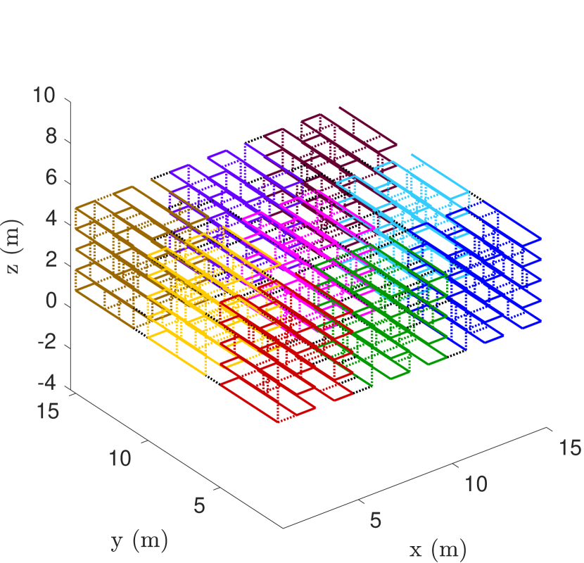
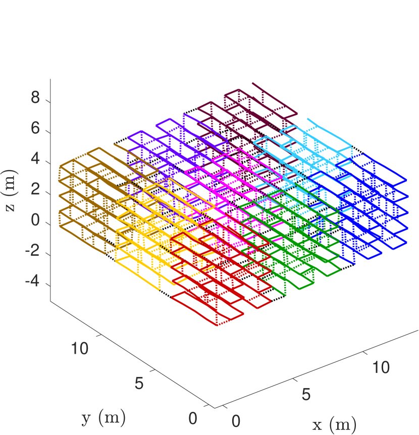
When evaluating our approach and baseline methods, we use the following performance metrics. First, we compute the optimality gap , where is the optimal value of the centralized SDP relaxation computed using SE-Sync [12]. In the (typical) case that the SDP relaxation is exact, the rounded PGO estimates returned by both our approach and SE-Sync will achieve a zero optimality gap (to within numerical tolerances). Additionally, when evaluating convergence rates of local search methods, we compute the evolution of the Riemannian gradient norm, which quantifies how fast the iterates are converging to a first-order critical point. Lastly, in some experiments, we also compute the translational and rotational root mean square errors (RMSE) with respect to the solution of SE-Sync. Given two sets of translations , the translational RMSE is based on the standard distance after aligning in the same frame. Given two sets of rotations , we define the rotational RMSE to be,
| (65) |
where is the orbit distance for defined in SE-Sync [12, Appendix C.1]. Although we measure rotational and translational errors separately, both still give meaningful metrics of the overall PGO solution. This is especially true for rotational RMSE, since we know that given rotation estimates, the corresponding optimal translations can be computed in closed-form [12].
The rest of this section is organized as follows. In Section 8.1, we evaluate our distributed local search methods, specifically RBCD and its accelerated version RBCD++, when solving the rank-restricted relaxations of PGO. Then, in Section 8.2, we evaluate the proposed distributed verification scheme. Lastly, in Section 8.3, we evaluate our complete distributed certifiably correct PGO algorithm (Algorithm 2).
8.1 Evaluations of Distributed Local Search
We first evaluate the performance of the proposed RBCD and RBCD++ algorithms when solving the rank-restricted relaxations (Problem 21). Recall that this serves as the central local search step in our overall Riemannian Staircase algorithm. By default, we set the relaxation rank to , and enable parallel execution as described in Section 4.4.
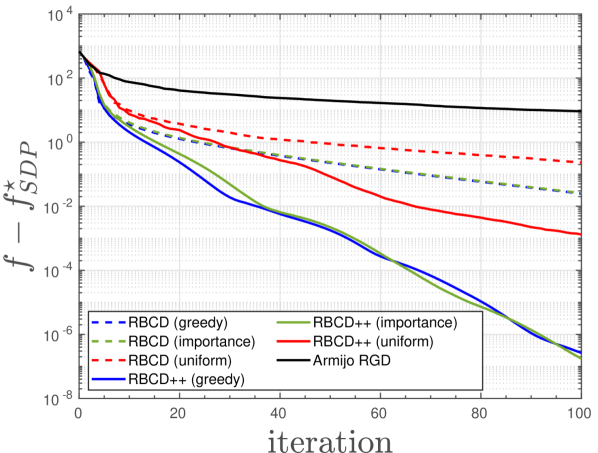
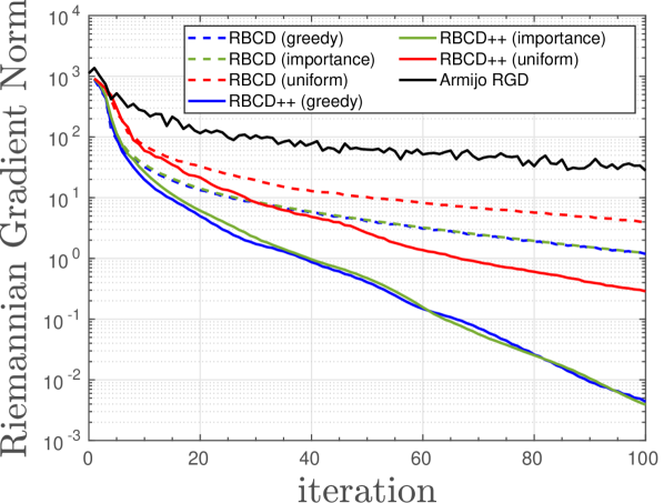
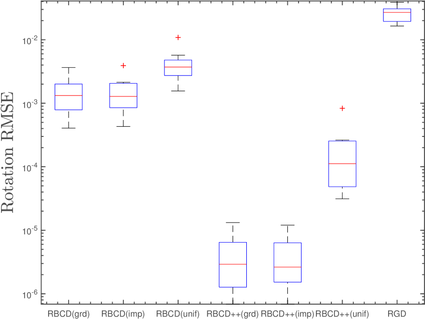
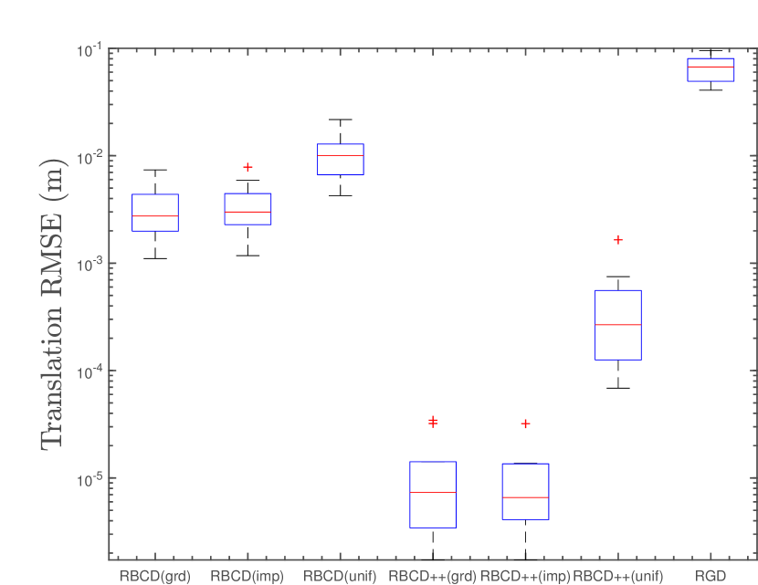
Figure 5 shows the performance on our 9 robot scenario shown in Figure 4. We report the performance of our proposed methods using all three block selection rules proposed in Section 4.1: uniform sampling, importance sampling, and greedy selection. For reference, we also compare our performance against the Riemannian gradient descent (RGD) algorithm with Armijo’s backtracking line search implemented in Manopt [65]. As the results demonstrate, both RBCD and RBCD++ dominate the baseline RGD algorithm in terms of convergence speed and solution quality. As expected, importance sampling and greedy block selection also lead to faster convergence compared to uniform sampling. Furthermore, RBCD++ shows significant empirical acceleration and is able to converge to the global minimum with high precision using only 100 iterations. Note that in this experiment, we choose to report convergence speed with respect to iteration number, because it is directly linked to the number of communication rounds required during distributed optimization. For completeness, we also note that the average runtime of BlockUpdate (implemented based on a modified version of the trust-region solver in Manopt [65]) is s.
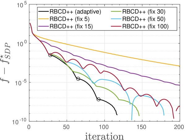
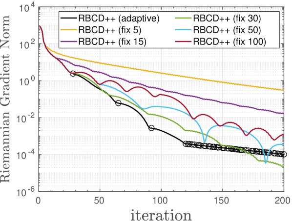
In Figure 5, we report the performance of RBCD++ with the default adaptive restart scheme (see Algorithm 5). As we have discussed in Remark 8, a less expensive and hence more practical restart scheme is simply to reset Nesterov’s acceleration after a fixed number of iterations; this scheme is typically referred to as fixed restart in the literature. In Figure 6, we compare adaptive restart with fixed restart on a random instance of our simulation. For fixed restart, we use different restart frequency ranging from every 5 to every 100 iterations. We observe that with a short restart period (e.g., 5), convergence of RBCD++ is significantly slowed down. This result is expected, as frequent restarting essentially removes the effect of acceleration from the iterations of RBCD++. In the extreme case of restarting at every iteration, the algorithm essentially reduces to RBCD. On the other hand, long restart period (e.g., 100) also has a negative impact, and we observe that the overall convergence displays undesirable oscillations. Finally, we find that a suitably chosen restart period (e.g., 30) demonstrates a superior convergence rate that is similar to the adaptive restart scheme.
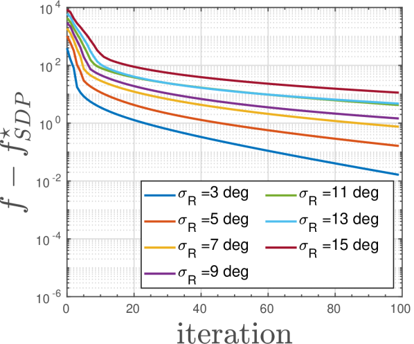
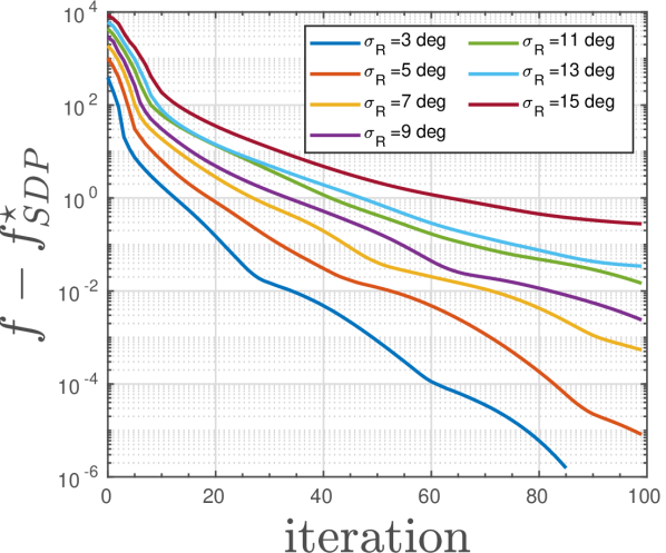
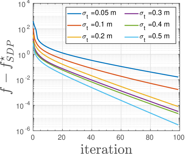
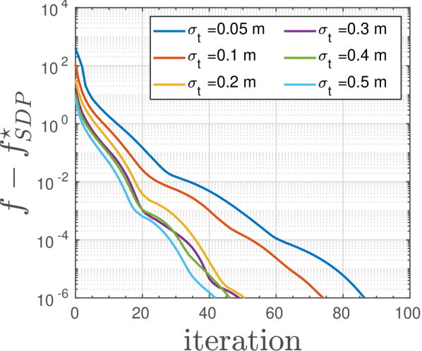
On the same 9 robot scenario, we also report the convergence of RBCD and RBCD++ (using greedy selection) under increasing measurement noise, shown in Figure 7. As expected, as rotation noise increases, the convergence rates of both RBCD and RBCD++ are negatively impacted. On the other hand, we observe that increasing translation noise actually leads to better convergence behavior, as shown in Figure 7(c)-7(d). To explain these observations, we conjecture that increasing rotation noise and decreasing translation noise magnify the ill conditioning of the optimization problem. Qualitatively similar results were also reported in [12] (decreasing translational noise was observed to increase SE-Sync’s wall-clock time).
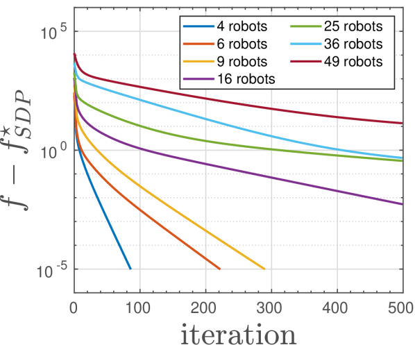
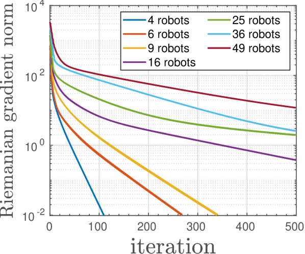
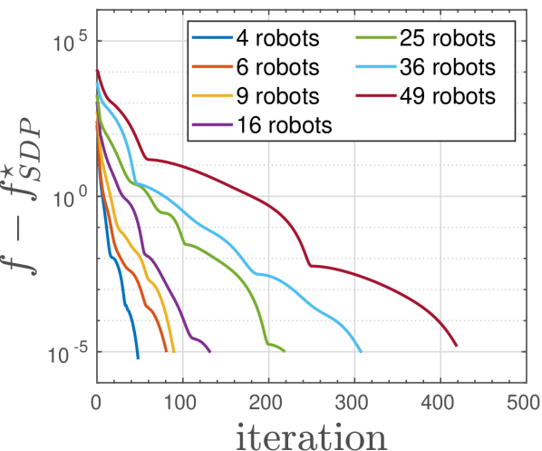
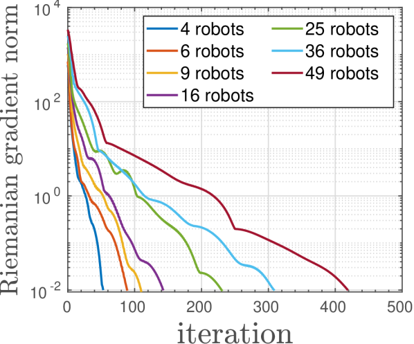
Lastly, we evaluate the scalability of RBCD and RBCD++ (both with greedy block selection) as the number of robots increases from 4 to 49 in the simulation. As each robot has 125 poses, the maximum size of the global PGO problem is 6125. Figure 8 reports the convergence speeds measured in Riemannian gradient norm. Both RBCD and RBCD++ are reasonably fast for small number of robots. Nevertheless, the non-accelerated RBCD algorithm begins to show slow convergence as the number of robots exceeds 16. In comparison, our accelerated RBCD++ algorithm shows superior empirical convergence speed, even in the case of 49 robots. We note that in this case although RBCD++ uses 400 iterations to achieve a Riemannian gradient norm of , the actual optimality gap (Figure 8(c)) decreases much more rapidly to , which indicates that our solution is very close to the global minimum.
8.2 Evaluations of Distributed Verification
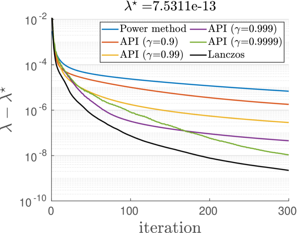
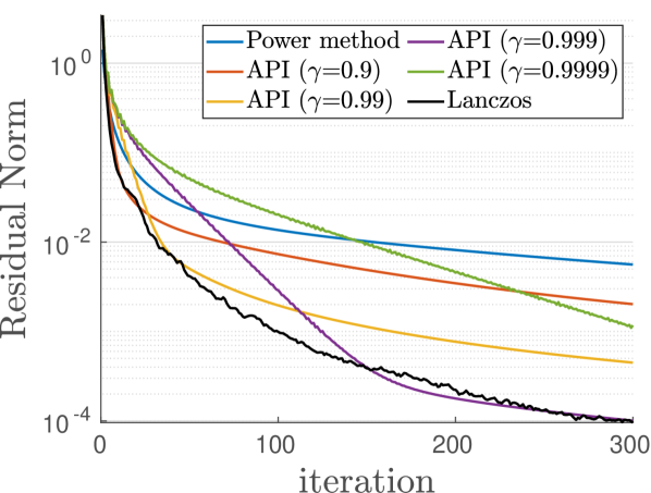
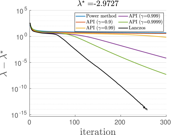
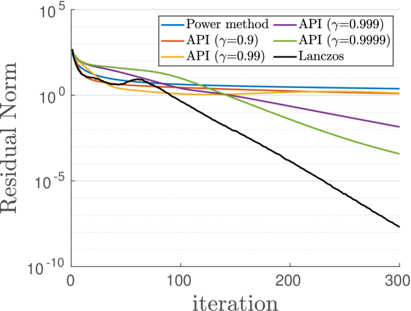
In this section we evaluate our proposed distributed verification method. Recall from Section 6 that the bulk of work happens when using accelerated power iteration to compute the dominant eigenpair of the spectrally-shifted dual certificate matrix . We thus examine the efficiency of this process, and compare the performance of accelerated power iteration against standard power method and the centralized Lanczos procedure. We note that since and share the same set of eigenvectors, in our experiment we still report results based on the estimated eigenvalues of .
From Remark 13, the accelerated power iteration achieves the theoretical optimal rate when the employed momentum term satisfies , where is the second dominant eigenvalue of . Since we know that belongs to a tight cluster whenever is globally optimal, we expect that typically . Using this insight, in our experiment we first estimate by multiplying with a factor that is close to one, i.e., . Subsequently we use this estimated value to set the momentum term,
| (66) |
We design two test cases using the Killian court dataset. In the first case, we verify the global minimizer computed by SE-Sync [12]. By Theorem 6, the dual certificate matrix must be positive semidefinite. Furthermore, since always has a nontrivial nullspace spanned by the rows of the corresponding primal solution, we expect the minimum eigenvalue of to be zero in this case. Indeed, when computing this using the eigs function in MATLAB, the final value (denoted as in Figure 9(a)) is close to zero to machine precision. Figure 9(a) shows how fast each method converges to , where we use an initial eigenvector estimate obtained by (slightly) randomly perturbing a row of the global minimizer [52]. Figure 9(b) shows the corresponding Ritz residual for the estimated eigenvector . Assuming is normalized, this is given by,
| (67) |
As the results suggest, with a suitable choice of , accelerated power iteration is significantly faster than the standard power method. Furthermore, in this case convergence speed is close to the Lanczos procedure.
In the second case, we verify a suboptimal first-order critical point obtained by running RBCD++ with using random initialization. We verify that the minimum eigenvalue of is negative (), which is consistent with the prediction of Theorem 6. In this case, we observe that using a random initial eigenvector estimate leads to better convergence compared to obtaining the initial estimate from a perturbed row of the primal solution. Intuitively, using the perturbed initial guess would cause the iterates of power method to be “trapped” for longer period of time near the zero eigenspace spanned by the rows of . Figure 9(c)-9(d) shows results generated with random initial eigenvector estimate. Note that there is a bigger performance gap between accelerated power iteration and the Lanczos algorithm. However, we also note that in reality, full convergence is actually not needed in this case. Indeed, from Theorem 6, we need only identify some direction that satisfies in order to escape the current suboptimal solution.
8.3 Evaluations of Complete Algorithm (Algorithm 2)
So far, we have separately evaluated the proposed local search and verification techniques. In this section, we evaluate the performance of the complete DC2-PGO algorithm (Algorithm 2) that uses distributed Riemannian Staircase (Algorithm 1) to solve the SDP relaxation of PGO. By default, at each level of the Staircase we use RBCD++ with greedy selection to solve the rank-restricted relaxation until the Riemannian gradient norm reaches . Then, we use the accelerated power method to verify the obtained solution. To set the momentum term, we employ the same method introduced in the last section with in (66). The accelerated power iteration is deemed converged when the eigenvector residual defined in (67) reaches .
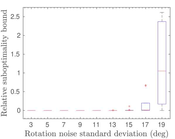
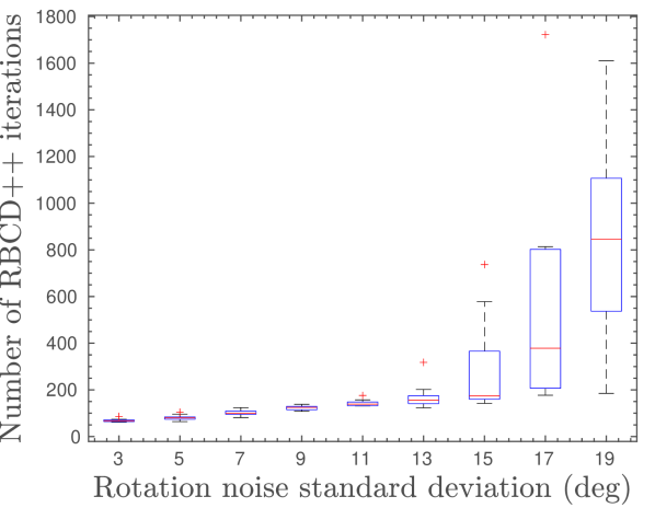
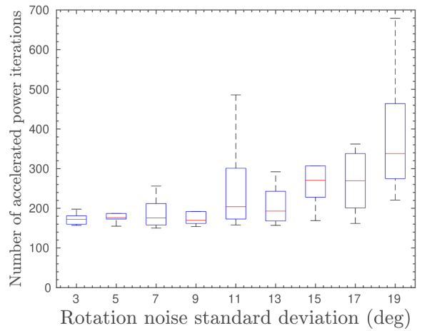
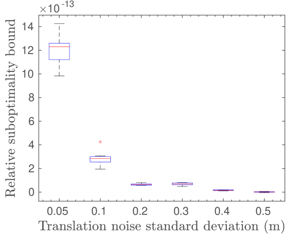
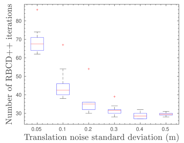
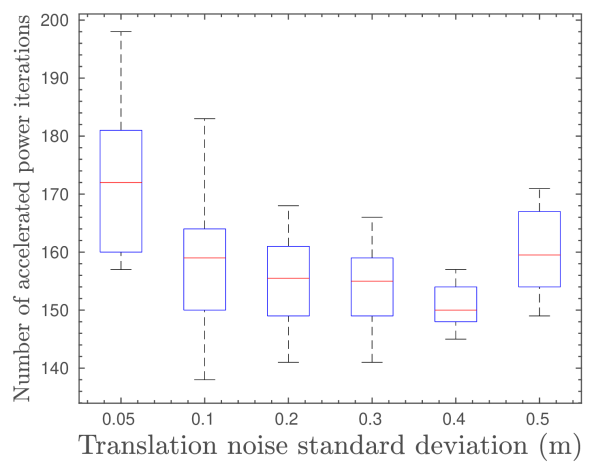
We first examine the exactness of the SDP relaxation in the 9-robot scenario shown in Figure 4 under increasing measurement noise. Recall that DC2-PGO returns both a rounded feasible solution as well as the optimal value of the SDP relaxation . To evaluate exactness, we record the upper bound on the relative suboptimality of , defined as . We note that a zero suboptimality bound means that the SDP relaxation is exact and the solution is a global minimizer. As shown in the first column of Figure 10, DC2-PGO is capable of finding global minimizers for all translation noise considered in our experiments, and for rotation noise up to 11 degree, which is still much larger than noise magnitude typically encountered in SLAM. The middle and right columns of Figure 10 show the total number of iterations used by RBCD++ and accelerated power method, across all levels of the staircase. Interestingly, we observe that changing measurement noise has a greater impact for distributed local search compared to distributed verification.
| Dataset | # Vertices | # Edges | Objective | Local Search Iterations | ||||
| Init. | SE-Sync [12] | DGS [5] | DC2-PGO | DGS [5] | DC2-PGO | |||
| Killian Court (2D) | 808 | 827 | 229.0 | 61.15 | 63.52 | 61.22 | 27105 | 189 |
| CSAIL (2D) | 1045 | 1171 | 31.50 | 31.47 | 31.49 | 31.47 | 10 | 197 |
| Intel Research Lab (2D) | 1228 | 1483 | 396.6 | 393.7 | 428.89 | 393.7 | 10 | 187 |
| Manhattan (2D) | 3500 | 5453 | 369.0 | 193.9 | 242.05 | 194.0 | 1585 | 785 |
| KITTI 00 (2D) | 4541 | 4676 | 1194 | 125.7 | 269.87 | 125.7 | 1485 | 2750 |
| City10000 (2D) | 10000 | 20687 | 5395 | 638.6 | 2975.2 | 638.7 | 2465 | 1646 |
| Parking Garage (3D) | 1661 | 6275 | 1.64 | 1.263 | 1.33 | 1.311 | 25 | 47 |
| Sphere (3D) | 2500 | 4949 | 1892 | 1687 | 1689 | 1687 | 300 | 53 |
| Torus (3D) | 5000 | 9048 | 24617 | 24227 | 24246 | 24227 | 100 | 88 |
| Cubicle (3D) | 5750 | 16869 | 786.0 | 717.1 | 726.69 | 717.1 | 45 | 556 |
| Rim (3D) | 10195 | 29743 | 8177 | 5461 | 5960.4 | 5461 | 515 | 1563 |
Lastly, we evaluate DC2-PGO on benchmark datasets. Figure 11 shows the globally optimal solutions returned by our algorithm. In Table 1, we compare the performance of DC2-PGO against the centralized certifiable SE-Sync algorithm [12], as well as the state-of-the-art distributed Gauss-Seidel (DGS) algorithm by Choudhary et al. [5]. For DGS, we set the SOR parameter to 1.0 as recommended by the authors, and for which we also observe stable performance in general. On all datasets, DC2-PGO is able to verify its solution as the global minimizer. We note that on some datasets, the final objective value is slightly higher than SE-Sync. This is due to the looser convergence condition used in our distributed local search: for RBCD++ we set the gradient norm threshold to , while for SE-Sync we set the threshold to in order to obtain a high-precision reference solution.888In general it is not reasonable to expect RBCD or RBCD++ to produce solutions that are as precise as those achievable by SE-Sync in tractable time, since the former are first-order methods, while the latter is second-order. On the other hand, DC2-PGO is clearly more advantageous compared to DGS, as it returns a global minimum, often with fewer iterations. The performance of DGS is more sensitive to the quality of initialization, as manifested on the Killian Court and City10000 datasets. In addition, while our local search methods are guaranteed to reduce the objective value at each iteration, DGS does not have this guarantee as it is operating on a linearized approximation of the PGO problem.
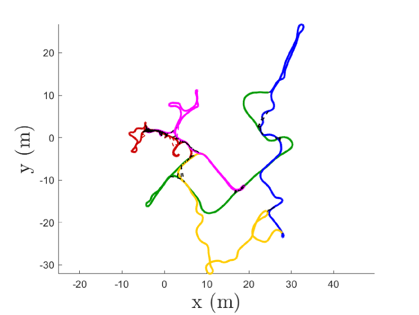
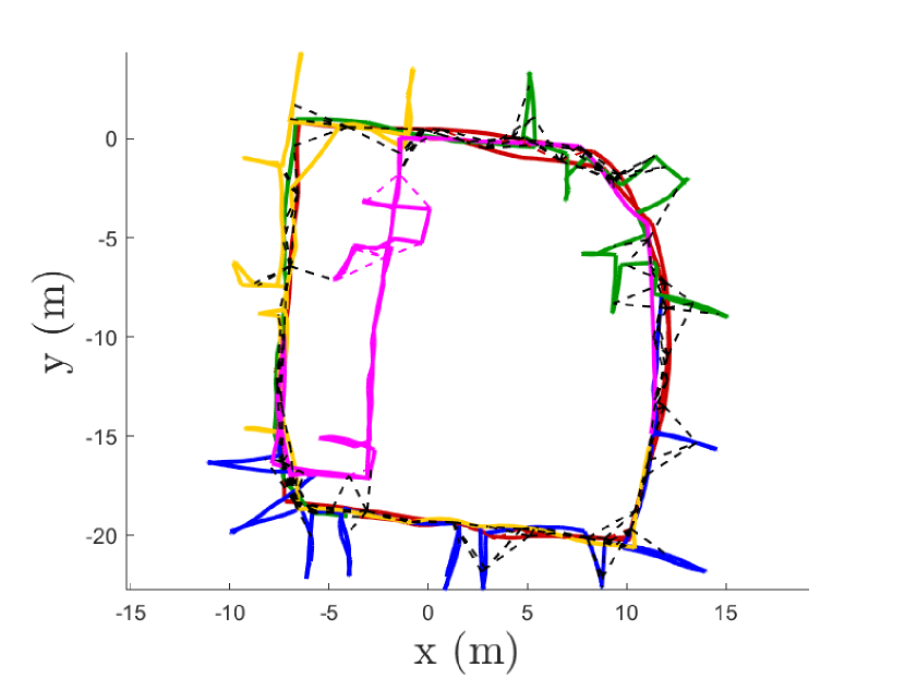
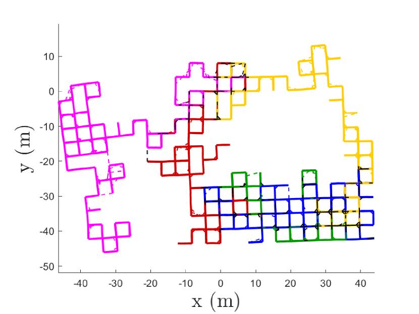
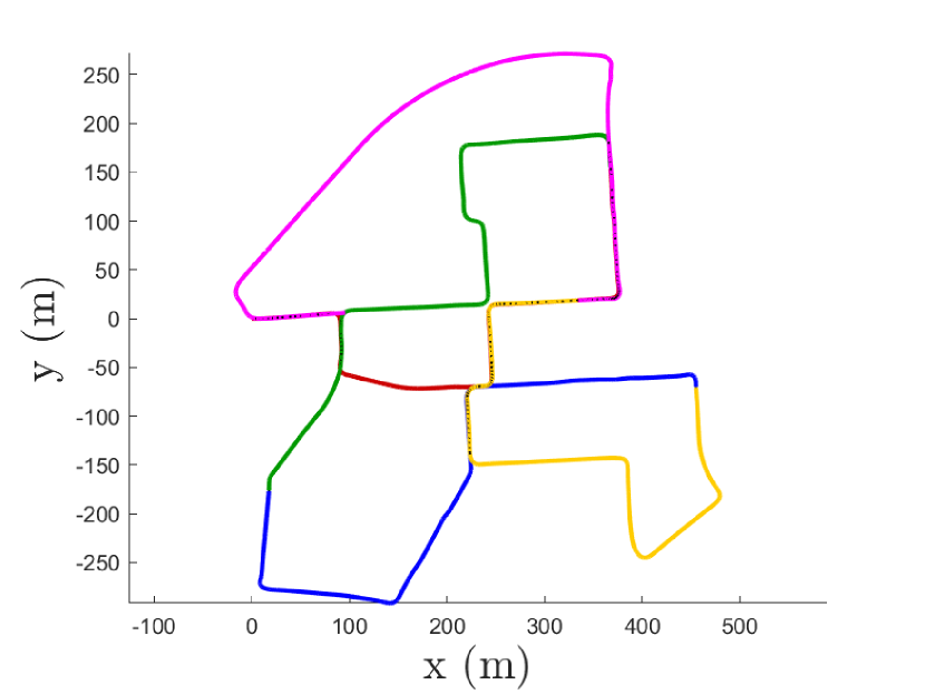
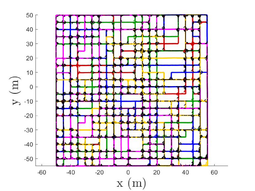
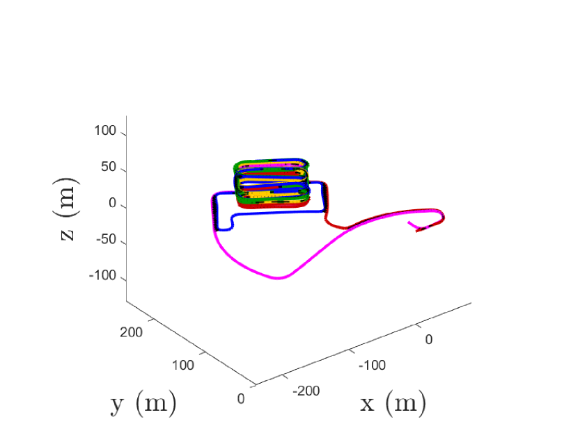
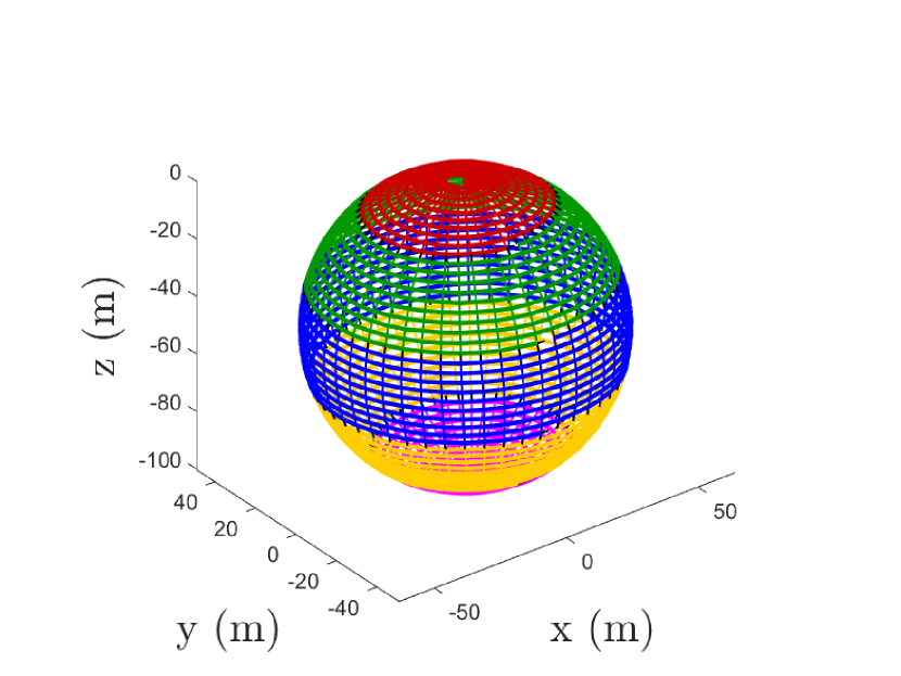
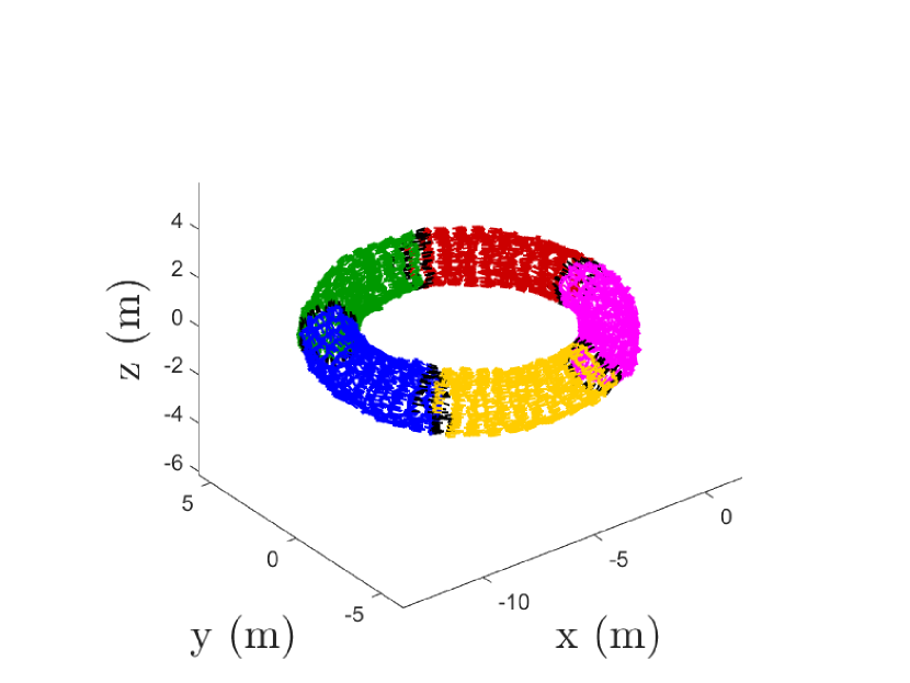
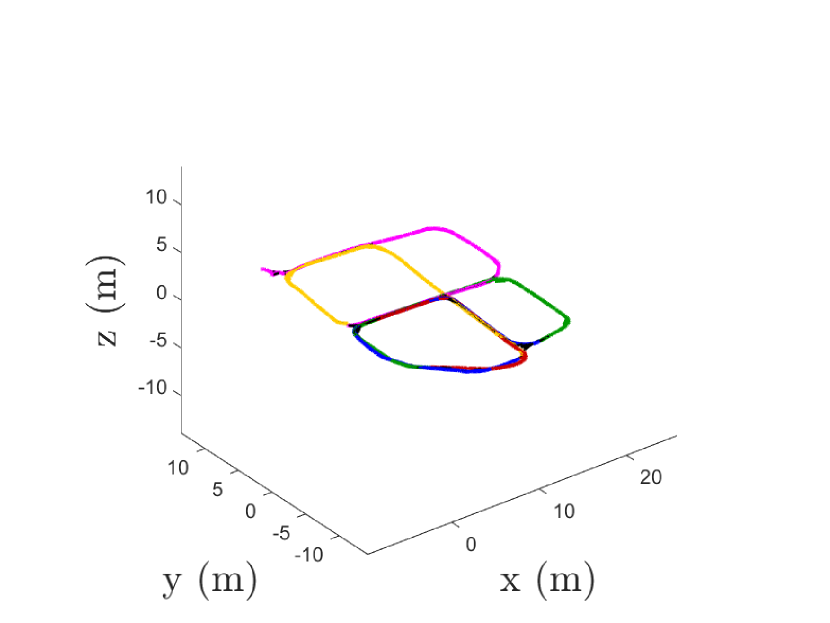
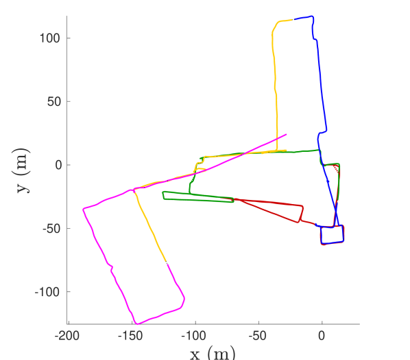
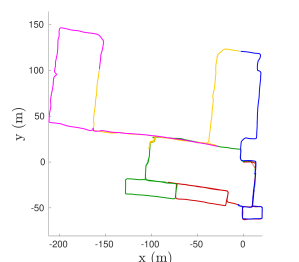
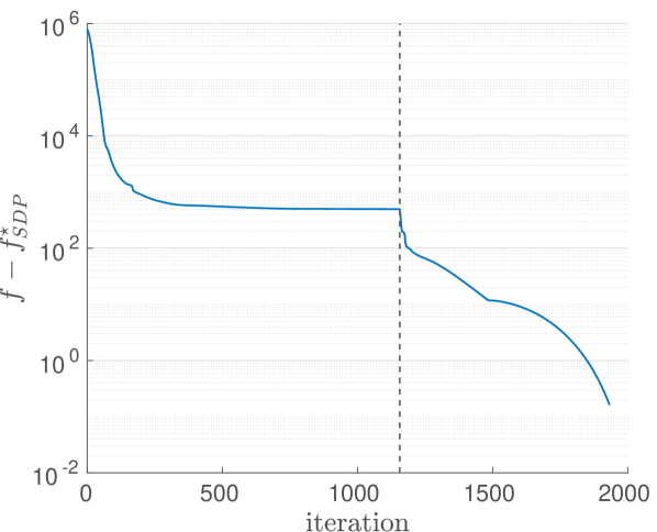
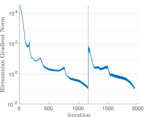
To further demonstrate the uniqueness of our algorithm as a global solver, we show that it is able to converge to the global minimum even from random initialization. This is illustrated using the Killian court dataset in Figure 12. Due to the random initialization, the first round of distributed local search at rank converges to a suboptimal critical point. This can be seen in Figure 12(c), the the optimality gap at (first 1068 iterations) converges to a non-zero value. From distributed verification, our algorithm detects the solution as a saddle point and is able to escape and converges to the correct global minimizer at rank . This can be clearly seen in Figure 12(d), where escaping successfully moves the iterate to a position with large gradient norm, from where local search can successfully descend to the global minimizer.
9 Conclusion
In this work we proposed the first certifiably correct algorithm for distributed pose-graph optimization. Our method is based upon a sparse semidefinite relaxation of the pose-graph optimization problem that we prove enjoys the same exactness guarantees as current state-of-the-art centralized methods [12]: namely, that its minimizers are low-rank and provide globally optimal solutions of the original PGO problem under moderate noise. To solve large-scale instances of this relaxation in the distributed setting, we leveraged the existence of low-rank solutions to propose a distributed Riemannian Staircase framework, employing Riemannian block coordinate descent as the core distributed optimization method. We proved that RBCD enjoys a global sublinear convergence rate under standard (mild) conditions, and can be significantly accelerated using Nestorov’s scheme. We also developed the first distributed solution verification and saddle escape algorithms to certify the optimality of critical points recovered via RBCD, and to descend from suboptimal critical points if necessary. Finally, we provided extensive numerical evaluations, demonstrating that the proposed approach correctly recovers globally optimal solutions under moderate noise, and outperforms alternative distributed methods in terms of estimation quality and convergence speed.
In the future, we plan to study approaches to further improve iteration complexity on hard problem instances. Another interesting direction is the design of certifiably correct distributed algorithm that can handle outlier measurements in CSLAM and CNL. While robustness has gained increasing attention in multi-robot SLAM [66, 30], recent certifiably robust approaches such as [67] are still restricted to centralized setting due to high computational requirements.
Lastly, similar to other distributed algorithms, the performance of DC2-PGO is expected to degrade as network conditions deteriorate (e.g., as network topology becomes sparser or delay increases). To this end, our recent work [68] studied convergence of distributed PGO under communication delay. In general, however, designing distributed SLAM systems that better handle real-world communication challenges remains an important direction for future research.
Acknowledgments
The authors would like to thank Luca Carlone for fruitful discussions that led to this work. This work was supported in part by the NASA Convergent Aeronautics Solutions project Design Environment for Novel Vertical Lift Vehicles (DELIVER), by ONR under BRC award N000141712072, and by ARL DCIST under Cooperative Agreement Number W911NF-17-2-0181.
References
- Schmuck and Chli [2018] P. Schmuck and M. Chli, “CCM-SLAM: Robust and efficient centralized collaborative monocular simultaneous localization and mapping for robotic teams,” Journal of Field Robotics, 2018.
- Deutsch et al. [2016] I. Deutsch, M. Liu, and R. Siegwart, “A framework for multi-robot pose graph slam,” in 2016 IEEE International Conference on Real-time Computing and Robotics (RCAR). IEEE, 2016, pp. 567–572.
- Morrison et al. [2016] J. G. Morrison, D. Gálvez-López, and G. Sibley, “Moarslam: Multiple operator augmented rslam,” in Distributed autonomous robotic systems. Springer, 2016, pp. 119–132.
- Kim et al. [2010] B. Kim, M. Kaess, L. Fletcher, J. Leonard, A. Bachrach, N. Roy, and S. Teller, “Multiple relative pose graphs for robust cooperative mapping,” in 2010 IEEE International Conference on Robotics and Automation. IEEE, 2010, pp. 3185–3192.
- Choudhary et al. [2017] S. Choudhary, L. Carlone, C. Nieto, J. Rogers, H. I. Christensen, and F. Dellaert, “Distributed mapping with privacy and communication constraints: Lightweight algorithms and object-based models,” The International Journal of Robotics Research, vol. 36, no. 12, pp. 1286–1311, 2017.
- Fan and Murphey [2020a] T. Fan and T. Murphey, “Majorization minimization methods to distributed pose graph optimization with convergence guarantees,” arXiv preprint arXiv:2003.05353, 2020.
- Cunningham et al. [2013] A. Cunningham, V. Indelman, and F. Dellaert, “DDF-SAM 2.0: Consistent distributed smoothing and mapping,” in 2013 IEEE International Conference on Robotics and Automation, May 2013, pp. 5220–5227.
- Cunningham et al. [2010] A. Cunningham, M. Paluri, and F. Dellaert, “DDF-SAM: Fully distributed SLAM using constrained factor graphs,” in 2010 IEEE/RSJ International Conference on Intelligent Robots and Systems. IEEE, 2010, pp. 3025–3030.
- Fan and Murphey [2019] T. Fan and T. D. Murphey, “Generalized proximal methods for pose graph optimization,” in The International Symposium on Robotics Research, 2019.
- Carlone et al. [2015a] L. Carlone, D. M. Rosen, G. Calafiore, J. J. Leonard, and F. Dellaert, “Lagrangian duality in 3D SLAM: Verification techniques and optimal solutions,” in 2015 IEEE/RSJ International Conference on Intelligent Robots and Systems (IROS), 2015, pp. 125–132.
- Bandeira [2016] A. S. Bandeira, “A note on probably certifiably correct algorithms,” Comptes Rendus Mathematique, 2016.
- Rosen et al. [2019] D. M. Rosen, L. Carlone, A. S. Bandeira, and J. J. Leonard, “SE-Sync: A certifiably correct algorithm for synchronization over the special euclidean group,” The International Journal of Robotics Research, vol. 38, no. 2-3, pp. 95–125, 2019.
- Briales and Gonzalez-Jimenez [2017] J. Briales and J. Gonzalez-Jimenez, “Cartan-Sync: Fast and global SE(d)-synchronization,” IEEE Robotics and Automation Letters, 2017.
- Boumal [2015] N. Boumal, “A Riemannian low-rank method for optimization over semidefinite matrices with block-diagonal constraints,” arXiv preprint arXiv:1506.00575, 2015.
- Boumal [2020] ——, “An introduction to optimization on smooth manifolds,” Available online, Aug 2020. [Online]. Available: http://www.nicolasboumal.net/book
- Absil et al. [2009] P.-A. Absil, R. Mahony, and R. Sepulchre, Optimization algorithms on matrix manifolds. Princeton University Press, 2009.
- Burer and Monteiro [2003] S. Burer and R. D. C. Monteiro, “A nonlinear programming algorithm for solving semidefinite programs via low-rank factorization,” Math. Program., vol. 95, pp. 329–357, 2003.
- Absil et al. [2007] P.-A. Absil, C. G. Baker, and K. A. Gallivan, “Trust-region methods on riemannian manifolds,” Foundations of Computational Mathematics, vol. 7, no. 3, pp. 303–330, 2007.
- Khosoussi et al. [2016] K. Khosoussi, S. Huang, and G. Dissanayake, “A sparse separable SLAM back-end,” IEEE Transactions on Robotics, vol. 32, no. 6, pp. 1536–1549, 2016.
- Singer [2011] A. Singer, “Angular synchronization by eigenvectors and semidefinite programming,” Applied and Computational Harmonic Analysis, 2011.
- Bandeira et al. [2017] A. S. Bandeira, N. Boumal, and A. Singer, “Tightness of the maximum likelihood semidefinite relaxation for angular synchronization,” Mathematical Programming, vol. 163, no. 1, pp. 145–167, May 2017.
- Eriksson et al. [2019] A. Eriksson, C. Olsson, F. Kahl, and T. Chin, “Rotation averaging with the chordal distance: Global minimizers and strong duality,” IEEE Transactions on Pattern Analysis and Machine Intelligence, 2019.
- Dellaert et al. [2020] F. Dellaert, D. Rosen, J. Wu, R. Mahony, and L. Carlone, “Shonan rotation averaging: Global optimality by surfing ,” in European Conference on Computer Vision (ECCV), 2020.
- Hartley et al. [2013] R. Hartley, J. Trumpf, Y. Dai, and H. Li, “Rotation averaging,” International Journal of Computer Vision, 2013.
- Tron [2012] R. Tron, Distributed optimization on manifolds for consensus algorithms and camera network localization. The Johns Hopkins University, 2012.
- Tron and Vidal [2014] R. Tron and R. Vidal, “Distributed 3-D localization of camera sensor networks from 2-D image measurements,” IEEE Transactions on Automatic Control, vol. 59, no. 12, pp. 3325–3340, Dec 2014.
- Tron et al. [2016] R. Tron, J. Thomas, G. Loianno, K. Daniilidis, and V. Kumar, “A distributed optimization framework for localization and formation control: Applications to vision-based measurements,” IEEE Control Systems Magazine, vol. 36, no. 4, pp. 22–44, 2016.
- Singer and Shkolnisky [2011] A. Singer and Y. Shkolnisky, “Three-dimensional structure determination from common lines in cryo-em by eigenvectors and semidefinite programming,” SIAM Journal on Imaging Sciences, vol. 4, no. 2, pp. 543–572, 2011.
- Cieslewski et al. [2018] T. Cieslewski, S. Choudhary, and D. Scaramuzza, “Data-efficient decentralized visual SLAM,” in 2018 IEEE International Conference on Robotics and Automation (ICRA). IEEE, 2018, pp. 2466–2473.
- Lajoie et al. [2019] P.-Y. Lajoie, B. Ramtoula, Y. Chang, L. Carlone, and G. Beltrame, “DOOR-SLAM: Distributed, online, and outlier resilient SLAM for robotic teams,” arXiv preprint arXiv:1909.12198, 2019.
- Bertsekas and Tsitsiklis [1989] D. P. Bertsekas and J. N. Tsitsiklis, Parallel and distributed computation: numerical methods. Prentice hall Englewood Cliffs, NJ, 1989, vol. 23.
- Fan and Murphey [2020b] T. Fan and T. Murphey, “Majorization minimization methods to distributed pose graph optimization with convergence guarantees,” 2020.
- Nesterov [2012a] Y. Nesterov, “Efficiency of coordinate descent methods on huge-scale optimization problems,” SIAM Journal on Optimization, vol. 22, no. 2, pp. 341–362, 2012. [Online]. Available: https://doi.org/10.1137/100802001
- O’Donoghue and Candes [2012] B. O’Donoghue and E. Candes, “Adaptive restart for accelerated gradient schemes,” Foundations of Computational Mathematics, vol. 15, 04 2012.
- Wright [2015] S. J. Wright, “Coordinate descent algorithms,” Math. Program., vol. 151, no. 1, pp. 3–34, Jun. 2015. [Online]. Available: https://doi.org/10.1007/s10107-015-0892-3
- Nutini et al. [2017] J. Nutini, I. Laradji, and M. Schmidt, “Let’s make block coordinate descent go fast: Faster greedy rules, message-passing, active-set complexity, and superlinear convergence,” 2017.
- Mareček et al. [2015] J. Mareček, P. Richtárik, and M. Takáč, “Distributed block coordinate descent for minimizing partially separable functions,” in Numerical Analysis and Optimization. Springer, 2015, pp. 261–288.
- Beck and Tetruashvili [2013] A. Beck and L. Tetruashvili, “On the convergence of block coordinate descent type methods,” SIAM journal on Optimization, vol. 23, no. 4, pp. 2037–2060, 2013.
- Nesterov [2012b] Y. Nesterov, “Efficiency of coordinate descent methods on huge-scale optimization problems,” SIAM Journal on Optimization, vol. 22, no. 2, pp. 341–362, 2012.
- Duckett et al. [2000] T. Duckett, S. Marsland, and J. Shapiro, “Learning globally consistent maps by relaxation,” in Robotics and Automation, 2000. Proceedings. ICRA’00. IEEE International Conference on, vol. 4. IEEE, 2000, pp. 3841–3846.
- Frese et al. [2005] U. Frese, P. Larsson, and T. Duckett, “A multilevel relaxation algorithm for simultaneous localization and mapping,” IEEE Transactions on Robotics, vol. 21, no. 2, pp. 196–207, 2005.
- Hartley et al. [2011] R. Hartley, K. Aftab, and J. Trumpf, “L1 rotation averaging using the weiszfeld algorithm,” in CVPR 2011. IEEE, 2011, pp. 3041–3048.
- Wen et al. [2009] Z. Wen, D. Goldfarb, S. Ma, and K. Scheinberg, “Row by row methods for semidefinite programming,” Industrial Engineering, pp. 1–21, 2009.
- Wang et al. [2017] P.-W. Wang, W.-C. Chang, and J. Z. Kolter, “The mixing method: low-rank coordinate descent for semidefinite programming with diagonal constraints,” arXiv preprint arXiv:1706.00476, 2017.
- Erdogdu et al. [2018] M. A. Erdogdu, A. Ozdaglar, P. A. Parrilo, and N. D. Vanli, “Convergence rate of block-coordinate maximization burer-monteiro method for solving large SDPs,” arXiv preprint arXiv:1807.04428, 2018.
- Tian et al. [2019a] Y. Tian, K. Khosoussi, and J. P. How, “Block-coordinate minimization for large SDPs with block-diagonal constraints,” arXiv preprint arXiv:1903.00597, 2019.
- Giamou et al. [2018] M. Giamou, K. Khosoussi, and J. P. How, “Talk resource-efficiently to me: Optimal communication planning for distributed loop closure detection,” in IEEE International Conference on Robotics and Automation (ICRA), 2018. [Online]. Available: https://arxiv.org/abs/1709.06675
- Tian et al. [2019b] Y. Tian, K. Khosoussi, and J. P. How, “A resource-aware approach to collaborative loop closure detection with provable performance guarantees,” arXiv preprint arXiv:1907.04904, 2019.
- Javanmard et al. [2016] A. Javanmard, A. Montanari, and F. Ricci-Tersenghi, “Phase transitions in semidefinite relaxations.” Proceedings of the National Academy of Sciences (PNAS), 2016.
- Lynch [1996] N. A. Lynch, Distributed algorithms. Elsevier, 1996.
- Boumal et al. [2018] N. Boumal, P.-A. Absil, and C. Cartis, “Global rates of convergence for nonconvex optimization on manifolds,” IMA Journal of Numerical Analysis, vol. 39, no. 1, pp. 1–33, 02 2018.
- Rosen and Carlone [2017] D. Rosen and L. Carlone, “Computational enhancements for certifiably correct SLAM,” in IEEE/RSJ International Conference on Intelligent Robots and Systems (IROS), 2017, workshop on “Introspective Methods for Reliable Autonomy”.
- Barenboim and Elkin [2009] L. Barenboim and M. Elkin, “Distributed ()-coloring in linear (in ) time,” in Proceedings of the forty-first annual ACM symposium on Theory of computing. ACM, 2009, pp. 111–120.
- Schneider and Wattenhofer [2010] J. Schneider and R. Wattenhofer, “A new technique for distributed symmetry breaking,” in Proceedings of the 29th ACM SIGACT-SIGOPS symposium on Principles of distributed computing. ACM, 2010, pp. 257–266.
- Rosen [2020] D. M. Rosen, “Scalable low-rank semidefinite programming for certifiably correct machine perception,” in Intl. Workshop on the Algorithmic Foundations of Robotics (WAFR), Jun. 2020.
- Vandenberghe and Boyd [1996] L. Vandenberghe and S. Boyd, “Semidefinite programming,” SIAM Review, vol. 38, no. 1, pp. 49–95, Mar. 1996.
- Boumal et al. [2016] N. Boumal, V. Voroninski, and A. S. Bandeira, “The non-convex burer–monteiro approach works on smooth semidefinite programs,” in Proceedings of the 30th International Conference on Neural Information Processing Systems. USA: Curran Associates Inc., 2016, pp. 2765–2773.
- Journée et al. [2010] M. Journée, F. Bach, P.-A. Absil, and R. Sepulchre, “Low-rank optimization on the cone of positive semidefinite matrices,” SIAM J. Optim., vol. 20, no. 5, pp. 2327–2351, 2010.
- Golub and Loan [1996] G. Golub and C. V. Loan, Matrix Computations, 3rd ed. Baltimore, MD: Johns Hopkins University Press, 1996.
- Saad [1980] Y. Saad, “On the rates of convergence of the Lanczos and the block-Lanczos methods,” SIAM J. Numer. Anal., vol. 17, no. 5, pp. 687–706, Oct. 1980.
- de Sa et al. [2018] C. de Sa, B. He, I. Mitliagkas, C. Ré, and P. Xu, “Accelerated stochastic power iteration,” in Proc. Mach. Learn. Res., no. 84, 2018, pp. 58–67.
- Konolige et al. [2010] K. Konolige, G. Grisetti, R. Kümmerle, W. Burgard, B. Limketkai, and R. Vincent, “Sparse pose adjustment for 2d mapping,” in IEEE/RSJ Intl. Conf. on Intelligent Robots and Systems (IROS), 2010.
- Martinec and Pajdla [2007] D. Martinec and T. Pajdla, “Robust rotation and translation estimation in multiview reconstruction,” in IEEE Conference on Computer Vision and Pattern Recognition, Minneapolis, MN, Jun. 2007, pp. 1–8.
- Carlone et al. [2015b] L. Carlone, R. Tron, K. Daniilidis, and F. Dellaert, “Initialization techniques for 3D SLAM: A survey on rotation estimation and its use in pose graph optimization,” in 2015 IEEE International Conference on Robotics and Automation (ICRA), May 2015, pp. 4597–4604.
- Boumal et al. [2014] N. Boumal, B. Mishra, P.-A. Absil, and R. Sepulchre, “Manopt, a Matlab toolbox for optimization on manifolds,” Journal of Machine Learning Research, 2014. [Online]. Available: http://www.manopt.org
- Mangelson et al. [2018] J. G. Mangelson, D. Dominic, R. M. Eustice, and R. Vasudevan, “Pairwise consistent measurement set maximization for robust multi-robot map merging,” in Proceedings of the IEEE International Conference on Robotics and Automation, Brisbane, Australia, May 2018, pp. 1–8.
- Lajoie et al. [2019] P. Lajoie, S. Hu, G. Beltrame, and L. Carlone, “Modeling perceptual aliasing in SLAM via discrete-continuous graphical models,” IEEE Robotics and Automation Letters, vol. 4, no. 2, pp. 1232–1239, April 2019.
- Tian et al. [2020] Y. Tian, A. Koppel, A. S. Bedi, and J. P. How, “Asynchronous and parallel distributed pose graph optimization,” IEEE Robotics and Automation Letters, vol. 5, no. 4, pp. 5819–5826, 2020.
- Gallier [2010] J. Gallier, “The Schur complement and symmetric positive semidefinite (and definite) matrices,” Dec. 2010, unpublished note, available online: http://www.cis.upenn.edu/~jean/schur-comp.pdf.
- Edelman et al. [1999] A. Edelman, T. A. Arias, and S. T. Smith, “The geometry of algorithms with orthogonality constraints,” SIAM J. Matrix Anal. Appl., vol. 20, no. 2, pp. 303–353, Apr. 1999.
Appendix A Exactness of SDP Relaxation
| # | Problem Description | Cost Function | Domain | Constraints |
|---|---|---|---|---|
| 13 | MLE for PGO | (13a) | – | |
| 18 | Full SDP Relaxation of PGO | |||
| 19 | Rotation-only SDP Relaxation for PGO | |||
| 21 | Rank-Restricted Full SDP for PGO | – | ||
| 69 | Rank-Restricted Rotation-only SDP for PGO | – |
In this section, we provide additional discussions of our SDP relaxation (Problem 18) and give a proof of its exactness under low noise. To facilitate the discussion, we summarize all problems that are considered in this work in Table 2. The core idea behind our proof is to establish certain equivalence relations with the rotation-only SDP relaxation (Problem 19), which is first developed by Rosen et al. in SE-Sync [12]. To begin, we first define the cost matrix that appears in the rotation-only SDP; see also [12, Equation 20(b)].
| (68) |
In (68), is the rotation connection Laplacian, and is the graph Laplacian of the pose graph with edges weighted by the translation measurement weights . The remaining two matrices and are formed using relative translation measurements. The exact expressions of these matrices are given in equations (13)-(16) in [12] and are omitted here. Let us consider the rank-restricted version of the rotation-only SDP defined below.
Problem 5 (Rotation-only Rank-restricted SDP for Pose Synchronization [12]).
| (69) |
Problem 69 and the sparse rank-restricted relaxation we solve in this paper (Problem 21) are intimately connected. The following lemma precisely characterizes this connection, and also provides an important tool for proving subsequent theorems in this section.
Lemma 2 (Connections between Problems 21 and 69).
Let be a first-order critical point of Problem 21. Let and be block matrices constructed from the Stiefel and Euclidean elements of , respectively. Then:
-
(i)
The translations satisfy:
(70) -
(ii)
is a first-order critical point of Problem 69, and
-
(iii)
Let denote the symmetric -block-diagonal matrix constructed by extracting the nonzero diagonal blocks from the Lagrange multiplier matrix defined in (49a):
(71) (72) (see also (3)). Then the Lagrange multiplier matrix:
(73) for the simplified (rotation-only) Problem 69 (cf. [12, eq. (107)]) satisfies:
(74) - (iv)
- (v)
Proof.
Using the definition of the connection Laplacian matrix in Problem 21 (see [13, Appendix II]), it can be shown that the cost function in Problem 21 can be expanded into the following,
| (75) |
Using (75), we may rewrite the cost function in a way that separates the Euclidean (translation) variables from the Stiefel (rotation) variables:
| (76) |
| (77) |
Above, the operator concatenates columns of the input matrix into a single vector. A detailed derivation for (76) is already presented in [12, Appendix B] for the case when . For , the derivation is largely identical with minor modifications to the dimensions of certain matrices, and thus is omitted. We make an additional remark that the new data matrix (77) is related to the original connection Laplacian via a permutation of the columns and rows.
Let us define and . From (76), we derive the Euclidean gradients of with respect to and , respectively.
| (78) | ||||
| (79) |
Similarly, we also have:
| (80) |
Part (i): Since is a first-order critical point, the Euclidean gradient with respect to the translations must be zero. In light of (78), we need to identify such that,
| (81) |
Using the general fact that , we may vectorize the above system of equations to,
| (82) |
Define and . Since is the Kronecker product between the Laplacian of a connected graph and the identity matrix, it holds that and the kernel of is spanned by the columns of . We can equivalently express as (cf. [12, Equation (76)]),
| (83) |
Let be an arbitrary null vector of . Consider the inner product between and ,
| (84) |
The last equality is due to the fact that by the definition of ; see equation (15) in [12]. Therefore, we have proven that . Since is symmetric positive-semidefinite, it holds that . Thus, the system of linear equations (82) admits infinitely many solutions, characterized by the following set,
| (85) |
Recalling the definitions of and , we can convert (85) back to matrix form (cf. [12, Equation (21)]):
| (86) |
Part (ii): Substituting the translation expression (86) into the Euclidean gradient with respect to (79), we obtain:
| (87) |
where in the second line we again used the fact that the all-s vector belongs to the null space of . Thus, we have shown that Problems 21 and 69 have the same Euclidean gradient with respect to the Stiefel elements . Since is a first-order critical point, the Riemannian gradient of with respect to is zero, which implies that:
| (88) |
i.e., is a first-order critical point of Problem 69. Finally, plugging the expression of into shows that .
Part (iii): The Lagrange multiplier matrices and for Problem 21 and Problem 69 are:
| (89) | ||||
| (90) |
see (49a) and [12, eq. (107)], respectively. Extracting and aggregating the nonzero diagonal blocks of (cf. (3)), we obtain:
| (91) |
where we have used (87) for the middle equality.
Part (iv): After permutation, the certificate matrix defined in (49b) can be written in the block form:
| (92) |
(cf. (77)). Since and , it follows from [69, Thm. 4.3] that if only if the following generalized Schur complement of with respect to is positive semidefinite:
| (93) |
Part (v): We show that Problem 69 is obtained from Problem 21 after analytically eliminating the translations . Consider the problem of minimizing the cost function (76) with respect to translations only (as a function of ). Since this is an unconstrained convex quadratic problem, we can minimize this cost first with respect to by setting the corresponding gradient to zero. In part (i) we identified the set of all translations (for a fixed ) satisfying this condition; see equation (86). After replacing in the original cost function (76) with any element from , we obtain the following rotation-only problem,
| (94) |
which is exactly Problem 69. This concludes our proof. ∎
A.1 Proof of Theorem 1
With Lemma 2 in place, we are ready to prove the equivalence relations between our SDP relaxation (Problem 18) and its rotation-only version (Problem 19), stated in Theorem 1 of the main paper.
Proof of Theorem 1.
We give a constructive proof where we show that from a minimizer to Problem 18 (full SDP relaxation), we can recover a minimizer to Problem 19 (rotation-only SDP relaxation) with the same rank, and vice versa. Without loss of generality, let . Consider the rank- factorization . Since is a feasible point for Problem 18, it can be readily verified that is an element of the product manifold (7). Let be obtained by stacking all rotational components of . We prove that is an optimal solution to Problem 19. To see this, first note that is an optimal solution to the rank-restricted SDP Problem 21. Therefore, by Lemma 2, it holds that,
| (95) |
Now, suppose is not an optimal solution to Problem 69. Then there exists such that . Once again, without loss of generality, let and consider the rank- factorization where . Now suppose is an optimal value for translations given (see (86)):
| (96) |
Let be obtained by combining and and define . Again by Lemma 2, it holds that,
| (97) |
The combination of (95) and (97) would imply that , which contradicts the starting assumption that is an optimal solution. Therefore must be an optimal solution with rank . To conclude the proof, note that using a similar argument, we can construct an optimal solution to Problem 18 from an optimal solution to Problem 19 with the same rank.
∎
A.2 Proof of Theorem 2
In this subsection, we formally prove the exactness guarantees of the SDP relaxation (Problem 18) used in this work, which is stated in Theorem 2 of the main paper.
Proof of Theorem 2.
By [12, Proposition 2], there exists a constant as a function of the noiseless data matrix of the rotation-only SDP relaxation (Problem 19), denoted as , such that if , the rotation-only SDP relaxation (Problem 19) admits a unique solution , where is a globally optimal rotation estimate to PGO (Problem 13). Let be an arbitrary minimizer to Problem 18. By Theorem 1, it holds that . Without loss of generality, let where . Consider the rank- factorization , where . Note that is a global minimizer to Problem 21, and hence by Lemma 2, it holds that,
| (98) |
Above, extracts the Stiefel elements from . Since Problem 19 admits a unique minimizer, (98) implies that is the same minimizer:
| (99) |
In addition, (99) also implies that . We may thus consider the -dimensional (thin) singular value decomposition . Let us define . Since , it holds that , and therefore consists of orthogonal matrices . By inspecting the first block row of this equality, we may further deduce that,
| (100) |
Multiplying both sides in (100) from the left by , such that the left hand side simplifies to .
| (101) |
Let us define . Since and , it holds that . Combining equality (101) for all yields the following compact equation.
| (102) |
Let contains the translations in . Since is a global minimizer, it is also a first-order critical point. Therefore, we can apply part (i) of Lemma 2 to relate with :
| (103) | |||||
| (104) | |||||
| (105) | |||||
In the last equality (105), we have defined . Notice that corresponds to a set of globally optimal translations. Finally, we note that the first block-row of the SDP solution may be expressed as,
| (106) | ||||
| (107) | ||||
| (108) |
In particular, can be obtained from via a global rigid body transformation with rotation and translation . Due to the global gauge symmetry of PGO, thus also is an optimal solution.
So far, we have proved that the SDP relaxation (Problem 18) is exact if its rotation-only counterpart (Problem 19) satisfies . To conclude the proof, let us consider the matrix defined in (77) and its latent value (i.e., constructed using noiseless relative transformation measurements). Note that and only differ in certain blocks,
| (109) |
Once again, the underline notation denotes the latent value of each data matrix. Matrices and summarize the measurement noise. Notice that the upper left block of is not affected by noise, since by construction it is always the (constant) translation-weighted graph Laplacian. Using the notation above, we can also express (68) as a function of and ,
| (110) |
Crucially, note that varies continuously with respect to the noise terms and . Therefore, as the noise tends to zero (equivalently, as tends to ), converges to its latent value . By definition, this guarantees the existence of a constant , such that implies . Finally, since the connection Laplacian and are related by a permutation of the rows and columns, it holds that,
| (111) |
which concludes the proof. ∎
Appendix B Convergence of RBCD and RBCD++
B.1 Proof of Lemma 1
Proof of Lemma 1.
Our proof largely follows the proof of Lemma 3.11 in [51]. By Assumption 38, the reduced cost over each block satisfies (38) globally with Lipschitz constant . To simplify our notation, we drop the iteration counter and use to represent the input into BlockUpdate (Algorithm 4). In addition, define . In the remaining proof, we also use to represent a tangent vector in . Using the simplified notation, consider the first trust-region subproblem solved in BlockUpdate (Algorithm 4).
| (112a) | ||||
| subject to | (112b) | |||
Recall that above is the initial trust-region radius. By Assumption 40, there exists such that for all . Define the constant,
| (113) |
Note that is the same constant that appears in the lower bound of the initial trust-region radius (Assumption 42).
We show that the required cost decrement in Lemma 1 is achieved by taking the so-called Cauchy step [51] in the first trust-region subproblem. By definition, the Cauchy step minimizes the model function (112) along the direction of the negative Riemannian gradient, i.e., . The step size can be determined in closed-form as,
| (114) |
A straightforward calculation (see [51, Lemma 3.7]) shows that the Cauchy step reduces the model function by at least,
| (115) |
Next, we need to relate the above model decrement (115) with the actual decrement of the cost function . For this, we show that the following ratio,
| (116) |
is close to zero. Note that in (116) we use the fact that, by definition, . We derive an upper bound on the numerator of (116) as follows,
| (117) | |||||
| (118) | |||||
| (119) | |||||
For the last inequality, we have used the Lipschitz-type gradient condition of for the first term, and the boundedness of for the second term. Plugging (115) and (119) into (116), we obtain,
| (115) and (119) | (120) | ||||
| (121) | |||||
| (122) |
In order to proceed, let us first impose an additional assumption that the initial trust-region radius is also bounded above by . Towards the end of this proof, we show how this assumption can be safely removed. Under this additional assumption, it holds that , and thus (122) implies,
| (123) |
In particular, is bigger than the acceptance threshold of in BlockUpdate (see Algorithm 4), and thus is guaranteed to be accepted. Consider the candidate solution corresponding to the Cauchy step . Using the definition of the pullback function, it holds that,
| (124) | |||||
| (125) | |||||
| (126) | |||||
| (127) | |||||
| (128) |
Therefore, we have proven that under the additional assumption that , the desired cost reduction can be achieved simply by taking the Cauchy step in the first trust-region subproblem. As we mention in Section 4, in practice, we use the truncated conjugate-gradient (tCG) algorithm to improve upon the initial Cauchy step. However, since each additional tCG iteration will strictly decrease the model function (see [16, Proposition 7.3.2]), we can show that the inequality (122) holds at all times, and thus the desired cost reduction is always achieved.
To complete the proof, we need to show that Algorithm 4 still achieves the desired cost reduction, even after removing the additional assumption that . To do so, note that after dropping this assumption, inequality (123) might fail to hold and as a result the Cauchy step can be rejected in the first iteration. However, by the mechanism of BlockUpdate (Algorithm 4), after each rejection the trust-region radius will be divided by four in the next iteration. Therefore, in the worst case, the trust-region radius will be within the interval after consecutive rejections, after which the Cauchy step is guaranteed to be accepted in the next trust-region subproblem.
∎
B.2 Proof of Theorem 45
Proof of Theorem 45.
We begin by using the sufficient descent property proved in Lemma 1, which states that after each BlockUpdate operation, the reduced cost is decreased by at least,
| (129) |
Recall that by design of the RBCD algorithm, at each iteration the values of all blocks other than remain unchanged. Denote the values of these fixed blocks as . By definition of the reduced cost , it is straightforward to verify that the decrease in exactly equals the decrease in the global cost ,
| (130) |
The above result directly implies that each iteration of RBCD reduces the global cost function by at least,
| (131) |
In the remaining proof, we use (131) to prove the stated convergence rate for each block selection rule.
Uniform Sampling.
In this case, the updated block is selected uniformly at random at each iteration.
Conditioned on all previously selected blocks , we can take expectation on both sides of (131) with respect to the current block .
| (132) |
Recall that all block are selected with equal probability, i.e., for all . Using this, we arrive at a simplified inequality that lower bounds the expected cost decrease by the squared gradient norm with respect to all variables .
| (133) |
We can use the above inequality (133) to bound the expected cost decrease over all iterations from to . To do so, we first write the overall cost reduction as a cascading sum, and then apply the law of total expectation on each expectation term that appears inside the sum.
| (134) |
Observe that each innermost conditional expectation is already bounded by our previous inequality (133). Plugging in this lower bound, we arrive at,
| (135) | ||||
| (136) |
To conclude the proof, we note that since is the global minimum, we necessarily have . This directly implies,
| (137) |
Rearranging the last inequality gives the desired convergence rate (44).
Importance Sampling.
We start with the same procedure of taking conditional expectations on both sides of (131).
The only difference is that with importance sampling, at each iteration the block is selected with probability proportional to the squared gradient norm, i.e.,
.
Using this to expand the conditional expectation gives:
| (138) | ||||
| (139) | ||||
| (140) |
where we define for brevity. Applying the Cauchy-Schwarz inequality gives,
| (141) |
Rearranging the above inequality yields,
| (142) |
Combining (140) and (142) gives,
| (143) |
The rest of the proof is identical to the proof for uniform sampling.
Greedy Selection.
With greedy selection, we can perform a deterministic analysis.
Recall that at each iteration, the block with the largest squared gradient norm is selected.
Using this information inside our inequality (131), we arrive at,
| (144) | ||||
| (145) | ||||
| (146) |
A telescoping sum of the above inequalities from to gives,
| (147) | ||||
| (148) | ||||
| (149) |
Rearranging the last inequality gives (45). ∎
B.3 Proof of Theorem 48
Proof.
For the purpose of proving global first-order convergence, we only focus on the evolution of the sequence in RBCD++ (Algorithm 5). After each iteration, there are two possibilities depending on whether the adaptive restart condition (line 20) is triggered. If restart is not triggered, then by construction the current iteration must achieve a cost reduction that is at least,
| (150) |
On the other hand, if restart is triggered, then the algorithm would instead update the selected block using the default BlockUpdate method. In this case, using the same argument as the beginning of proof for Theorem 45, we can establish the following lower bound on global cost reduction.
| (151) |
Combining the two cases, we see that each iteration of RBCD++ decreases the global cost by at least,
| (152) | |||||
| (153) | |||||
| (154) | |||||
The above inequality serves as a lower bound on the global cost reduction after each iteration. Note that this lower bound is very similar to (131) used in the proof of Theorem 45. The only difference is the change of constant on the right hand side. From this point on, we can employ the same steps used in the proof of Theorem 45 to prove the desired convergence rates for all three block selection rules. ∎
B.4 Convergence on Problem 4
In this section, we address the convergence of RBCD and RBCD++ when solving the rank-restricted semidefinite relaxations of PGO (Problem 4). To apply the general convergence results in Section 5, we need to check that the required technical conditions are satisfied. Among these, we note that the Riemannian Hessian operator (which we use as the user-specified map in Algorithm 4) satisfies Assumption 39 due to the linearity of affine connections [16, Section 5.2]. In addition, Assumption 42 can be satisfied by choosing a sufficiently large initial trust-region radius. Therefore, to establish convergence, we are left to verify Assumption 38 (Lipschitz-type gradients for pullback) and Assumption 40 (boundedness of Riemannian Hessian).
B.4.1 Verifying Assumption 38
We now show that Assumption 38 is satisfied in Problem 4, i.e., the reduced cost function (27) corresponding to any block has Lipschitz-type gradient for pullbacks along the iterates of RBCD and RBCD++. In [51], Boumal et al. prove a simple condition for a function defined on a matrix submanifold to have Lipschitz-type gradient for pullbacks. For convenience, we include their result below.
Lemma 3 (Lemma 2.7 in [51]).
Let be a Euclidean space and let be a compact Riemannian submanifold of . Let be a retraction on (globally defined). If has Lipschitz continuous gradient then the pullbacks satisfy (38) globally with some constant independent of .
In our case, we need a generalized version of Lemma 3 that extend the result to product manifold with Euclidean spaces.
Lemma 4 (Extension of Lemma 3 to product manifolds with Euclidean spaces).
Let and be Euclidean spaces, and define . Let , where is a compact Riemannian submanifold of . Given and , define a retraction operator as: where is a globally defined retraction on and we employ the standard retraction for Euclidean space. If has bounded and Lipschitz continuous gradient, then the pullbacks satisfy (38) globally with some constant independent of ; i.e.,
| (155) |
Proof.
This proof is a straightforward generalization of the proof of Lemma 3. By assumption, the Euclidean gradient is Lipschitz continuous, which implies the existence of a constant such that for any ,
| (156) |
The above inequality is true in particular for any . In this case, the inner product that appears in the LHS of (156) can be expanded as,
| (157) | |||||
| (158) | |||||
| (159) | |||||
| (160) | |||||
Next, we use two facts: (1) the Riemannian gradient in Euclidean space is just the standard (Euclidean) gradient; and (2) the Riemannian gradient of submanifolds embedded in a Euclidean space is the orthogonal projection of the Euclidean gradient onto the tangent space ([16, Equation 3.37]). With these, the above equality can be further simplified to,
| (161) | ||||
| (162) |
Plugging (162) into (156) gives,
| (163) |
Applying the triangle and Cauchy-Schwarz inequalities and expanding yields,
| (164) | ||||
| (165) | ||||
| (166) |
Since we assume that the Euclidean gradient is bounded, there exists constant such that for all . In equations (B.3) and (B.4) in [51], Boumal et al. show that for the compact submanifold , the following inequalities hold,
| (167) | ||||
| (168) |
for some . Plugging (167) and (168) in (166) gives,
| (169) |
Let . From (169) it trivially holds that,
| (170) |
∎
Let us consider the reduced cost (27) as a function defined on the product manifold , where is the number of poses contained in block . Note that in the ambient (Euclidean) space, is a quadratic function of . Hence, its Euclidean gradient is Lipschitz continuous, with Lipschitz constant given by the maximum eigenvalue of . Next, we show that within any sublevel set of the global cost function , is also bounded for any block . Since by construction of the reduced cost function, it is equivalent to bound the global Euclidean gradient . Write out the individual rotation and translation components of ,
| (171) |
For any in the -sublevel-set, expanding yields,
| (172) |
Since the objective consists of a sum over squared terms, we can obtain a uniform upper bound on each single term. Specifically, for each edge , the associated relative translation cost is bounded by,
| (173) |
Note that when forming , the only terms that are potentially unbounded correspond to the translation terms , since the rotation terms are defined on compact search spaces. The Euclidean gradients of with respect to , , are given by,
| (174) | |||
| (175) | |||
| (176) |
By (173), the norms of (174)-(176) are bounded, which implies that the overall Euclidean gradient is bounded within the sublevel set. Applying Lemma 155, we have shown that has Lipschitz-type gradient for pullbacks within the sublevel set of .
Finally, note that both RBCD and RBCD++ are by construction descent methods, i.e., the sequence of iterates satisfies for any . For RBCD, this is true since we explicitly enforce that each block update should produce a function decrease that is at least a constant fraction of the model decrease (Algorithm 4, line 12). For RBCD++, this is also guaranteed by the adaptive restart condition (see Section 4.3). This property ensures that the sequence of iterates generated by RBCD or RBCD++ never leaves the initial sublevel set, and therefore Assumption 38 is satisfied.
B.4.2 Verifying Assumption 40
We can follow a similar strategy and show that the Riemannian Hessian operator is bounded at any iterate generated by RBCD and RBCD++, hence satisfying Assumption 40. Let denote the cost function in Problem 21, and denote the solution at iteration . From (5), it may be straightforwardly verified that for Problem 21, the Riemannian Hessian operator has the following explicit form:
| (177) |
Above, is the “dual certificate” matrix (49b) defined in Theorem 6, repeated below for convenience,
| (178) |
In particular, note that (177) implies the following equality,
| (179) |
Following the strategy in Section B.4.1, we now show that is bounded within the sublevel sets of . To make the presentation clear, we present the proof in three steps.
Step 1: Eliminating Global Translation Symmetry from .
To begin, we observe that the connection Laplacian in Problem 21 always has a null vector [13],
| (180) |
where stands for the vector of all ones. Intuitively, arises as a result of the global translation symmetry inherent in pose-graph optimization. We note that although is a single vector, it actually accounts for the complete set of translational symmetries which has dimension . More precisely, adding a multiple of on the -th row of () corresponds to applying a global translation along the -th unit direction. Let us consider projecting each row of our decision variable onto the subspace orthogonal to . In matrix notation, this operation can be written as a matrix product , where is a projection matrix defined as follows.
| (181) |
Note that after projection, it holds that for some vector . Substitute this decomposition into the second term of (178),
| (182) | ||||
| (183) | ||||
| (184) |
In (184), we have used the linearity of the operator (3). Consider defined in (184) as a -by- block-structured matrix. Using the special structure of , we can verify that for each diagonal block of , its top-left -by- submatrix is always zero. Thus, applying zeros out this term and it holds that,
| (185) |
Equation (185) proves the intuitive result that the dual certificate matrix is invariant to any global translations applied to .
Step 2: Bounding within the sublevel set of .
We now prove that for all for which , the spectral norm is upper bounded by a constant which only depends on . In light of (185), for the purpose of bounding , we can assume without loss of generality that . This simply means that each row of is orthogonal to , which implies that , i.e., the translations are centered at zero. Recall the bound (173) we have obtained for translation terms in the previous section. Using triangle inequality, we can move to the right hand side, so that we obtain an upper bound on the relative translation between and ,
| (186) | |||||
| (187) | |||||
| (188) | |||||
Taking the square of the above bound and summing over all edges in the pose graph, it holds that,
| (189) |
Note that the constant only depends on and the input measurements. Let be the vector formed by concatenating all . The left hand side of (189) can be written in matrix form as , where is the (unweighted) Laplacian of the pose graph . Since is connected, the Laplacian has a rank-1 null space spanned by the all-ones vector . Correspondingly, has a rank- null space spanned by the columns of . Crucially, using our assumption that , it can be readily checked that is orthogonal to this null space. Therefore, we can obtain a lower bound on using the smallest positive eigenvalue of , which coincides with the algebraic connectivity of , denoted as ,
| (190) |
Combine this inequality with (189), we have thus shown that,
| (191) |
Since is guaranteed to be positive as the graph is connected, we can divide both sides by . After taking the square root, we obtain the following bound on the translations,
| (192) |
Recall that contains translations in addition to “lifted” rotations . Since is an element of the Stiefel manifold, the norm of in the ambient space is always a constant. This implies that the Frobenius norm is bounded. Finally, using the fact that as defined in (178) is a continuous operator together with (179), it holds that the induced operator norm of on the tangent space is bounded within the sublevel set.
Step 3: Bounding the Riemannian Hessian along iterates of RBCD and RBCD++.
Once again, since both RBCD and RBCD++ are descent methods by construction, any sequence of iterates will remain in the initial sublevel set. Therefore, by the result obtained in Step 2, there exists a constant (whose value only depends on ) that bounds the Riemannian Hessian at all iterations:
| (193) |
To complete the proof, we show that the reduced Riemannian Hessian, , at an arbitrary block is also bounded by . This is needed as during distributed local search, we apply BlockUpdate (Algorithm 4) on individual blocks instead of the full problem. Suppose for the sake of contradiction that there exists a tangent vector such that and . Let be the corresponding geodesic such that and . Define the scalar function . By standard results in differential geometry (e.g,. see [16]), it holds that .
Using the product structure of our manifold, we can associate with a corresponding geodesic on the overall manifold such that agrees with at the selected block coordinate and stays constant at all other blocks. Consider the tangent vector . By construction, the blocks of are given by,
| (194) |
As a result, we have . Define the scalar function and we have by construction that . This would then imply,
| (195) |
which is a contradiction.
Appendix C Proof of Theorem 3
In this subsection we establish the convergence properties of the (first-order) distributed Riemannian Staircase (Algorithm 1) described in Theorem 3.
If Algorithm 1 terminates finitely (case (i)) then there is nothing to prove, so henceforward let us assume that Algorithm 1 generates an infinite sequence of factors in line 7. Our overall strategy is to exploit the correspondence between the critical points of Problem 21 (rank-restricted full SDP) and the critical points of Problem 69 (rank-restricted rotation-only SDP) provided by Lemma 2, together with the compactness of the feasible set of the SE-Sync relaxation Problem 19, to control the behavior of this sequence. To that end, define:
| (196) |
where is the first-order critical point of Problem 69 obtained from as described by Lemma 2. In addition, let and denote the Lagrange multiplier matrices corresponding to and , respectively.
Since is an infinite sequence contained in the (compact) feasible set of Problem 19, it must contain a convergent subsequence , with limit point . Since the Lagrange multiplier is a continuous function of (see (90) and [12, eq. (107)]), it follows that likewise converges to a limit . By Lemma 2(iii) (cf. (74)), it follows that the subsequence of Lagrange multipliers for the full (translation-explicit) problem also converges to a limit point , and consequently so does the sequence of certificate matrices computed in line 8 of Algorithm 1:
| (197) |
Now, let us consider two cases, corresponding to whether is positive semidefinite.
Case 1: .
It is easy to check that since is by definition a first-order critical point. This shows that has a zero eigenvalue. Using this property, together with the fact that the eigenvalues of a matrix are continuous functions of and that , it holds that , thus proving (23).
To prove (22), note that by Lemma 2(iv), the certificate matrix associated with the limit point is likewise positive semidefinite, and therefore is a minimizer of Problem 19 [12, Thm. 7]. Since for all (Lemma 2(ii)), it follows that:
| (198) |
But then in fact we must have:
| (199) |
since the sequence of objective values is monotonically decreasing. This establishes that Theorem 3(ii) holds for the case .
Case 2: .
To finish the proof, we now show that in fact cannot occur. To do so, suppose for contradiction that , and define . Then there exists sufficiently large that for all . Our aim is to show that this upper bound (away from ) on the minimum eigenvalue of implies a lower bound on the achievable decrease in the objective value each time the saddle escape procedure in line 14 of Algorithm 1 is invoked with any ; since this occurs infinitely many times, this would imply that the optimal value of Problem 2 is , a contradiction.
We note that the following analysis holds at any rank of Algorithm 1 with . For the ease of reading, however, we will suppress in our notation and assume that and are clear from the context. Let be the critical point generated by the distributed Riemannian Staircase at iteration rank (Algorithm 1, line 7). Denote as the minimum eigenvalue of the corresponding certificate matrix (Algorithm 1, line 9), and as the corresponding second-order descent direction constructed (Algorithm 1, line 13). Recall that since , we have .
Consider the geodesic emanating from point with initial velocity (see Theorem 6). With a slight abuse of notation, we denote this geodesic as and it may be parameterized as follows,999Note that this map is in fact well-defined on all of because both the Stiefel manifold and are geodesically complete.
| (200) |
In addition, the cost function of Problem 21 restricted to :
| (201) |
From the integral form of Taylor’s Theorem, we have:
| (202) |
Differentiating and applying the chain rule, we arrive at,
| (203) |
where denotes the Frobenius inner product. Differentiating (203) again, we obtain,
| (204) |
Equations (203)-(204) hold by applying standard results for embedded manifolds; see [15, Chapters 3 and 5] and [16]. Furthermore, since is a geodesic, we may further show (see, e.g. [16, Section 5.4]) that its extrinsic acceleration is always orthogonal to the tangent space at . This means that the last term in (204) is identically zero since the Riemannian gradient at belongs to the tangent space at that point. Therefore, the second-order derivative further simplifies to,
| (205) |
The second equality makes use of (179). In particular, (203) and (205) show that (since is a critical point of ) and (since is nothing but in Theorem 6 and Remark 12). It follows from (202) that:
| (206) |
Thus, if we can exhibit scalars such that:
| (207) |
then (206) implies:
| (208) |
Since:
| (209) |
a straightforward calculation shows that the lower-bound for the reduction in the objective value attained in (208) is maximized by the steplength:
| (210) |
and that:
| (211) |
In consequence, by choosing a stepsize of:
| (212) |
when performing the retraction in the saddle escape procedure, we can guarantee that the objective is decreased by at least:
| (213) |
each time the saddle escape procedure is invoked, producing our desired contradiction.
It therefore suffices to exhibit fixed constants that will satisfy (207) for all invocations of the saddle escape procedure in line 14 with . Before proceeding, we make one simplifying assumption that will remain in effect throughout the remainder of the proof: we assume without loss of generality that all iterates are translated so that the sum of the translational components is , as in Section B.4.2.101010Note that this map leaves the objective invariant, and is an isometry of both the ambient Euclidean space and . Consequently, applying this transformation leaves all objective values and derivative norms invariant – we perform this transformation simply to achieve a parameterization that is more convenient for calculation. We now proceed in two stages: first we will identify an upper bound for the magnitude of on the sublevel set of the initial value of , and then a minimum distance from a given suboptimal critical point that we can retract along while still remaining inside this sublevel set.
Calculation of .
Recall the following notation for the sublevel sets of the cost function :
| (214) |
Our goal is to identify a fixed constant that upper bounds the magnitude of within the initial sublevel set, i.e.,
| (215) |
where is the initial value of the objective at the starting point supplied to Algorithm 1. From the second-order derivative (205), differentiate once again to obtain an explicit expression for . Here, we make use of the equality derived in (179) that relates the Riemannian Hessian and the certificate matrix ,
| (216) |
Fully expanding the differentiation yields,
| (217) |
where in the last step, we have used the symmetry of the certificate matrix to combine terms. We proceed to bound the two inner products in (217) separately.
To bound the first inner product, we first use the Cauchy-Schwarz inequality followed by applying the submultiplicative property of the Frobenius norm:
| (218) |
By construction of the descent direction (51), the velocity vector at satisfies . Since geodesics have constant speed, it thus holds that for all . Therefore, it suffices to bound the derivative of . Using the chain rule and repeatedly applying the submultiplicative property yields,
| (219) |
Above, denotes the operator norm of the linear map with respect to the Frobenius norm. A closer examination of the definition of in (3) reveals that in fact:111111This conclusion follows from the observation that sets off-diagonal block elements of its argument to zero, and extracts the symmetric parts of the on-diagonal blocks; consequently cannot increase the Frobenius norm of its argument, so that . Equality follows from the fact that fixes any symmetric block-diagonal matrix with the sparsity pattern appearing in (3).
| (220) |
Furthermore, since and is assumed to be centered, applying the results in Appendix B.4.2 (Step 2) shows that,
| (221) |
Finally, using that fact that the geodesic has constant speed , we establish the following constant bound for (219),
| (222) |
Now, let us return to (217) to bound the second inner product. Once again, we start by invoking the Cauchy-Schwarz inequality and the submultiplicative property of the Frobenius norm,
| (223) |
Since , applying the result of Appendix B.4.2 (Step 2) shows that there exists a constant such that . Next, we obtain an upper bound on the extrinsic acceleration. To this end, we note that in order to bound , it suffices to bound the extrinsic acceleration of each Stiefel element (since translations have zero extrinsic acceleration). Here, we use a result that gives an explicit characterization of along a geodesic on the Stiefel manifold [70, Eq. (2.7)]:
| (224) |
From the above characterization, it holds that,
| (225) |
where in the second inequality, we use the fact that . Therefore, is upper bounded as follows,
| (226) |
Combining these results yields a constant bound for the second inner product (223):
| (227) |
Finally, using the upper bounds (222) and (227) in (217) yields the final fixed upper bound ,
| (228) |
Calculation of :
Now we derive a such that for all and . Our approach is based upon deriving a simple upper bound for the magnitude of the change in objective value between two points and . To that end, consider:
| (229) |
Defining:
| (230) |
we may substitute in (229) to obtain:
| (231) |
We will use inequality (231) to derive a lower bound on the admissible steplength of the retraction applied at a critical point while still remaining inside the original sublevel set . Given the fact that and since, by definition, iff , it suffices to ensure that:
| (232) |
Applying inequality (231) with , and ,
| (233) |
From (232) and (233), for to remain in the sublevel set, it suffices to ensure that,
| (234) |
After rearranging and simplification, we can arrive at the following equivalent condition:
| (235) |
It is worth noting that each invocation of escaping procedure strictly reduces the objective, and thus here . We identify a constant lower bound for the right hand side of (235). To this end, let us view the right hand side as a function of . It can be straightforwardly verified that this function is nonincreasing. Since by (221) we have , it follows that the right hand side of (235) is always lower bounded the following constant,
| (236) |
Recalling (235), we have shown that remains in the sublevel set if the following holds:
| (237) |
Note that the above bound is expressed in terms of the chordal distance between and . To complete the proof, we note that the geodesic distance is always at least as large as the chordal distance. This means that for all , we have:
| (238) |
and thus , as claimed.