Geometric properties of galactic discs with clumpy episodes

Abstract

A scenario for the formation of the bi-modality in the chemical space [$\alpha$/Fe] vs [Fe/H] of the Milky Way was recently proposed in which $\alpha$-enhanced stars are produced early and quickly in clumps. Besides accelerating the enrichment of the medium with $\alpha$-elements, these clumps scatter the old stars, converting in-plane to vertical motion, forming a geometric thick disc. In this paper, by means of a detailed analysis of the data from smooth particle hydrodynamical simulations, we investigate the geometric properties (in particular of the chemical thick disc) produced in this scenario. For mono-age populations we show that the surface radial density profiles of high-[$\alpha$/Fe] stars are well described by single exponentials, while that of low-[$\alpha$/Fe] stars require broken exponentials. This break is sharp for young populations and broadens for older ones. The position of the break does not depend significantly on age. The vertical density profiles of mono-age populations are characterized by single exponentials, which flare significantly for low-[$\alpha$/Fe] stars but only weakly (or not at all) for high-[$\alpha$/Fe] stars. For low-[$\alpha$/Fe] stars, the flaring level decreases with age, while for high-[$\alpha$/Fe] stars it weakly increases with age (although with large uncertainties). All these properties are in agreement with observational results recently reported for the Milky Way, making this a plausible scenario for the formation of the Galactic thick disc.

1 Introduction

Galactic discs have two distinct photometric (or geometric) components, the thin and the thick discs, as first discovered by Burstein (1979) and Tsikoudi (1979) in external galaxies and further explored in more systematic studies by e.g. Yoachim & Dalcanton (2006, 2008a, 2008b) in the local universe and by Elmegreen & Elmegreen (2006); Elmegreen et al. (2017) at high redshifts. The same composite structure was also observed in the Milky Way (MW) since Yoshii (1982) and Gilmore & Reid (1983), with more recent results showing that in the Solar neighborhood the thin disc is mainly composed of younger stars which are poor in $\alpha$-elements and metal-rich, and with a characteristic scale height $h_{z1}\approx 0.3$ kpc. On the other hand, the thick disc is characterized by stars that are old, $\alpha$-enhanced and metal-poor, with vertical scale height $h_{z2}\approx 0.9$ kpc – see e.g. Bensby et al. (2005); Jurić et al. (2008).

The origin of the thick disc is still under active debate. Some works suggest the “upside-down” formation scenario, in which stars in the thick disc form while the gas is collapsing, i.e. they already form with their current height distribution. In a different scenario, Bournaud et al. (2009) observed that gas-rich young galaxies in simulations produce clumps that strongly scatter old stars, converting in-plane to vertical motion and giving origin to a thick disc. Bournaud et al. (2009) also concluded that a thick disc formed in this way has a constant scale height with galactocentric radius, i.e. it does not flare. Some observational support for this scenario was obtained by Comerón et al. (2011, 2014). Another interesting possibility for the formation of the thick disc is that these stars were brought (or produced in situ) by a major merger around 10 Gyr ago – see e.g. Belokurov et al. (2018); Helmi et al. (2018). The radial migration (of stars at corotation with transient spiral arms) was also proposed as a mechanism for the formation of the thick disc (Schönrich & Binney, 2009; Loebman et al., 2011), although it seems hard to reconcile this scenario with the bi-modality in the $\alpha$-abundance observed in the Milky Way (see below). On the other hand, radial migration is generally seen as a fundamental process determining the stellar radial distribution in the thin disc, in particular shaping the metallicity distribution function at different radii – see Hayden et al. (2015); Loebman et al. (2016).

Selecting mono-abundance populations (MAPs) in the chemical space [$\alpha$/Fe] vs [Fe/H], Bovy et al. (2012) concluded that the vertical density profiles of each of these MAPs in the MW is characterized by only one scale height, i.e. by a single exponential, finding no evidence of a chemically distinct thick disc and that the thin + thick disc structure only emerges as a consequence of superposing populations with different physical properties and dynamical histories. Similar conclusions were reached by Minchev et al. (2015), who propose that the geometric thick disc is a consequence of the superposition of many subpopulations, which are well fit by single exponentials with different flaring levels.

Closely related to the existence of the geometric thin and thick discs is the presence of a bi-modality in chemical space ([$\alpha$/Fe] vs [Fe/H]), defining a high-$\alpha$ and a low-$\alpha$ disc, as revealed by the APOGEE survey (Anders et al., 2014; Nidever et al., 2014; Hayden et al., 2015), showing the existence of a chemically distinct thick disc (the high-$\alpha$ stars), while the low-$\alpha$ region defines the chemical thin disc, although the association with the geometric discs is not exact. Some studies have associated this chemical bi-modality to the accretion events of the Galaxy (see e.g. Mackereth et al., 2018; Buck, 2020). However, its origin is still open.

Recently, Clarke et al. (2019) proposed that this bi-modality is associated to the occurrence of two distinct star formation channels in the disc: an early and fast star formation with fast chemical enrichment in clumps and a more continuous star formation dispersed in the disc. In this scenario, the high star formation rate density in clumps generates many supernovae type II, which rapidly enrich the medium with $\alpha$ elements. Additionally, as in the scattering process by giant molecular clouds proposed by Spitzer & Schwarzschild (1953), the clumps scatter the old, $\alpha$-rich stars, converting in-plane to vertical motion and promoting stars to high latitudes (essentially the same mechanism proposed by Bournaud et al., 2009). Clarke et al. (2019) ran hydrodynamical simulations employing a low stellar feedback efficiency, allowing the formation of clumps. They showed that these simulations naturally produce a chemical bi-modality with properties similar to the ones observed in the MW - see Fig. 5 from Clarke et al. (2019).

In the current work, we investigate the spatial distribution of the chemical discs formed by this simulation. In particular, we test whether, besides naturally producing the chemical bi-modality, the simple scenario explored in this simulation is also able to produce realistic geometric discs, particularly the thick disc. We apply several different cuts and compare the resulting density profiles with observational results. In Sec. 2, we describe the simulation. In Sec. 3, we introduce the different fitting models, which are compared to the simulation data in Sec.4. In Sec. 5, we compare our results with previous observational and simulation-based results and finally in Sec.6, we discuss and summarize the conclusions.

2 The Simulations

The simulation we use in this paper is the same as that explored and described by Clarke et al. (2019). Briefly, the model starts with a hot gas corona embedded in a spherical dark matter halo with a Navarro-Frenk-White (Navarro et al., 1997) halo with virial radius $r_{200}\simeq 200$ kpc and mass of $10^{12}M_{\odot}$. The gas has spin $\lambda=0.065$ (Bullock et al., 2001). The dark matter halo and gas corona both consist of $10^{6}$ particles initially. The gas cools via metal-line cooling (Shen et al., 2010), and settles into a disc, with stars forming from this gas when the temperature drops below 15,000 K and the density exceeds $1\mathrm{cm}^{-3}$. Feedback via supernova explosions uses the blastwave implementation described in Stinson et al. (2006), with 10% of the $10^{51}$ erg per supernova injected to the interstellar medium as thermal energy. Feedback via asymptotic giant branch stars is also taken into account. Following Agertz et al. (2009), we prevent gas cooling from dropping below our resolution by setting a gas pressure floor of $p_{floor}=3G\epsilon^{2}\rho^{2}$, where $G$ is Newton’s gravitational constant, $\epsilon$ is the softening length set at $50$ pc and $\rho$ is the gas particle’s density. Gas phase diffusion uses the method of Shen et al. (2010), reducing the scatter in the age-metallicity relation (Pilkington et al., 2012).

We evolve the model using the smooth particle hydrodynamics$+N$-body tree-code gasoline (Wadsley et al., 2004). The metal-line cooling results in clumps forming during early times in the model, as shown in Clarke et al. (2019). The final disc galaxy that forms has a rotational velocity of $242$ km/s at the Solar neighborhood, making it comparable to the MW. The final rotation curve and velocity dispersion profiles of the model are shown in Figure 2 of Clarke et al. (2019). We will refer to this simulation as FB10 (for feedback efficiency of $10\%$). Note that, although this simulated galaxy presents realistic properties in general, it is not intended to be a replica of the Milky Way. In particular, this simulated galaxy does not form a bar and has spatial scales with absolute values differing from those of the Milky Way.

In order to illustrate the effect of clumps on the chemistry of the model, we compare with a model in which the feedback from supernovae is set at $80\%$ of the $10^{51}$ erg per supernova. This feedback is 8 times higher than in our fiducial simulation; as a result clump formation is significantly suppressed in this simulation, as has been found in previous simulations (Hopkins et al., 2012; Genel et al., 2012; Buck et al., 2017; Oklopčić et al., 2017). We refer to this model as the high-feedback model (or FB80).

3 Modelling the Density profiles

In order to analyze the simulation data and make comparisons with observational results, we explore several fitting functions inspired by the models used in observational analyses. Our modelling varies in complexity reflecting approximately the chronological order in which these models were proposed by different studies. In all these models, the star-count density profiles are generically written as

$$\nu_{\star}(R,z|\theta)=\Sigma(R|\theta)\zeta(z|R,\theta),$$ (1)

where $R$ is the cylindrical radius, $z$ is the absolute latitude (vertical distance above or below the galactic plane), $\Sigma(R)$ is the surface density (units of length^-2), $\zeta(z|R)$ is the vertical density profile (units of length^-1) and $\theta$ is the set of parameters of the model.

We consider a total of five models (see Table 1), among which the first four have a a single exponential surface density profile , i.e.

$$\Sigma(R)=\frac{1}{A}e^{-R/h_{R}},$$ (2)

where $h_{R}$ is a free parameter and the constant $A$ is determined by the normalization condition

$$\int_{z_{min}}^{z_{max}}dz\int_{R_{min}}^{R_{max}}\nu_{\star}(R,z|\theta)\,2\pi RdR=N_{\star},$$ (3)

where $N_{\star}$ is the total number of star particles.

The first model (${\bf M1}$) considers a double exponential for the vertical profile, defining the thin and thick discs as first identified in the MW by Yoshii (1982) and Gilmore & Reid (1983):

$$\zeta(z|R)=\frac{1-\beta}{2h_{z1}}e^{-|z|/h_{z1}}+\frac{\beta}{2h_{z2}}e^{-|z|/h_{z2}},$$ (4)

where $h_{z1}$, $h_{z2}$ and $\beta$ are also free parameters.

Inspired by the results of Bovy et al. (2012), who found that the vertical density profile of mono-abundance populations in the MW were better described by single exponentials, our second model (${\bf M2}$) is characterized by

$$\zeta(z|R)=\frac{1}{2h_{z}}e^{-|z|/h_{z}}.$$ (5)

In Eqs. (4) and (5), the $R$-dependence is only formally present, since in these models the parameters $h_{z}$, $\beta$, $h_{z1}$ and $h_{z2}$ do not depend on $R$.

In our third model (${\bf M3}$), following the parameterization of Bovy et al. (2016), the vertical density profile is still a single exponential, Eq. (5), but now the vertical scale height is allowed to vary with radius $R$, i.e. to flare, as

$$h_{z}(R)=h_{z\odot}e^{R_{fl}^{-1}(R-R_{\odot})},$$ (6)

where the characteristic flaring radius $R_{fl}$ and the scale height at the Solar position $h_{z\odot}$ are also free parameters, while $R_{\odot}=8$ kpc is the radius of Solar position. Model ${\bf M4}$ is characterized by a double exponential vertical density profile, Eq. (4), but now the inner vertical scale height $h_{z1}$ is allowed to flare as in Eq. (6).

Finally, in model ${\bf M5}$ the vertical density profile is modeled as a single flaring exponential (as in model ${\bf M3}$, Eqs. 5 and 6), while the radial surface density is given by a broken exponential:

$$\Sigma(R)=\left\{\begin{array}[]{ll}\frac{1}{A_{1}}e^{-R/h_{R,\mathrm{in}}},&\textrm{if}\ R\leq R_{\mathrm{peak}}\\ \frac{1}{A_{2}}e^{-R/h_{R,\mathrm{out}}},&\textrm{if}\ R>R_{\mathrm{peak}},\end{array}\right.$$ (7)

where $h_{R,\mathrm{in}}$, $h_{R,\mathrm{out}}$ and $R_{\mathrm{peak}}$ are free parameters, while $A_{1}$ and $A_{2}$ are determined by the normalization condition, Eq. (3), and equating the two components at $R=R_{\mathrm{peak}}$. In order to allow the inner component to be an increasing function of radius, the inner slope $h_{R,\mathrm{in}}$ is allowed to assume positive or negative values. These models are listed in Table 1.

$\nu_{\star}(R,z|\theta)=\Sigma(R|\theta)\zeta(z|R,\theta)$	$\zeta(z|R,\theta)$	$\Sigma(R|\theta)$
M1	double exp., Eq. (4)	single exp., Eq. (2)
M2	single exp., Eq. (5)
M3	single flaring exp., Eqs. (5) and (6)
M4	double fl. inner exp., Eqs. (4) and (6)
M5	single flaring exp., Eqs. (5) and (6)	broken exp., Eq. (7)

Table 1: Summary of models fitted to the simulation data.

In order to test these models, in this work we perform Bayesian analyses where $\nu_{\star}(R,z|\theta)$ represents the probability to find a star particle at radius $R$ and absolute latitude $|z|$ or, considering the data altogether, the probability distribution for the data to be a sample realization of the model, given a fixed set of parameters $\theta$. In this approach, the likelihood function is defined as ${\cal L}\equiv\Pi_{i}\nu_{\star}(R_{i},z_{i}|\theta)$ and, more conveniently, we define the log-likelihood

$$\ln{\cal L}(\theta)=\sum_{i}\ln\left[\nu_{\star}(R_{i},z_{i}|\theta)\right],$$ (8)

where the sum runs over all star particles.

For all models described above, the log-likelihood is first maximized with a downhill simplex algorithm (Nelder & Mead, 1965) in order to obtain an initial estimate of the best fit parameters. These parameter values are then used as starting points to MCMC-sample the posterior distribution function with the emcee package (Foreman-Mackey et al., 2013). The MCMC-sampling allows us to better explore the parameter space and to estimate the uncertainties on the best fit parameters. In all analyses in this paper, the reported values of best fit parameters and their uncertainties are estimated as the median and the interval containing $68\%$ of the parameter sample, respectively.

In cases where more than one model is tested, the model comparison is made by means of the so-called Bayes factor

$$\ln B=\ln\left(\frac{E_{1}}{E_{2}}\right),$$ (9)

with positive (negative) values favouring model 1 (2). In this definition, $E_{1}$ and $E_{2}$ are the statistical evidences of each model, which in general can be approximated by

$$\ln E\approx\ln{\cal L}_{bf}-\frac{k}{2}\ln N,$$ (10)

where ${\cal L}_{bf}$ is the likelihood function evaluated in the best fit model, $N$ is the number of data points (star particles) and $k$ is the number of parameters in the model (the test penalizes models with larger numbers of parameters) – see e.g. Ivezić et al. (2014).

According to Kass & Raftery (1995), values $0\lesssim\ln B_{12}\lesssim 1$ deserve only a bare mention in favour of model 1, but model 1 is: weakly favoured for $1\lesssim\ln B_{12}\lesssim 3$, strongly favoured for $3\lesssim\ln B_{12}\lesssim 5$ and very strongly favoured for $\ln B_{12}\gtrsim 5$ (and the same for negative values in favour of model 2).

4 Results

4.1 Preliminaries: the geometric thick disc

In this section, we preliminarily show that the vertical density profile generated by the simulation has, broadly speaking, all the observed features of that of the Milky Way.

We select star particles at $t=10\ \mathrm{Gyr}$ within the cylinder ${6<R<10}$ kpc, ${|z|<3}$ kpc, resulting in a sample with ${N_{\star}=368,021}$ particles. Fig. 1 shows the normalized vertical density profile $(dn_{\star}/dz)/N_{\star}$ (where $n_{\star}$ is the number of star particles in each bin) in log-scale, split in 100 bins, with contours showing the Poisson uncertainty multiplied by 5. These plots are colour-coded by mean [O/Fe], mean [Fe/H], mean age and age dispersion, from left to right.

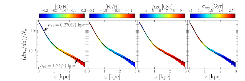
Figure 1: Density profile of the complete sample of star particles in the Solar neighborhood $6<R<10$ kpc, $|z|<3$ kpc. From left to right, the plots are colour-coded by [O/Fe], [Fe/H], age and age dispersion, respectively. Similarly to the MW (see Jurić et al., 2008), the data are well described by a double exponential model defining the geometric thin and thick discs, with scale height values shown in the left panel. The thick component ($|z|\gtrsim 1$kpc) is characterized by $\alpha$-rich, metal-poor and old populations, while the thin component ($|z|\lesssim 1$kpc) is $\alpha$-poor, metal-rich, young on average but with large age dispersions.

The vertical density profile has the characteristic double exponential shape observed in the MW (Gilmore & Reid, 1983), defining the geometric thin and thick discs. As in the MW, the geometric thin disc ($|z|\lesssim 1\ \mathrm{kpc}$) is dominated by stars that are poor in $\alpha$ elements (traced in the simulation by [O/Fe]), metal-rich and young. On the other hand, the geometric thick disc ($|z|\gtrsim 1\ \mathrm{kpc}$) is characterized by $\alpha$-rich, metal-poor and old stars. The right panel shows that while the thin disc is composed of stars with significantly different ages, the thick disc is much more uniform in age.

The (non-binned) data is then fit by model ${\bf M1}$, Eqs. (2) and (4). We assume flat priors for the inverse of parameters $h_{z1}$ and $h_{z2}$ and flat priors for $\beta$. The best fit values of the two vertical scale heights are $h_{z1}=0.270\pm 0.002$ kpc and $h_{z2}=1.24\pm 0.02$ kpc, as indicated in the left panel of Fig. 1. For the Milky Way, Jurić et al. (2008) found $h_{z1}\approx 0.3$ kpc and $h_{z2}\approx 0.9$ kpc.

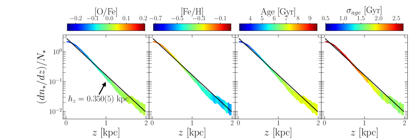
Figure 2: Density profile of the complete sample of star particles in the Solar neighborhood $6<R<10$ kpc, $|z|<3$ kpc for the simulation FB80. From left to right, the plots are colour-coded by [O/Fe], [Fe/H], age and age dispersion, respectively. We see that the data is described by a single exponential (black line), i.e., different from the MW, with no geometric thick disc.

For comparison, in Fig. 2 we show the vertical density profile generated in the simulation in which the stellar feedback efficiency is set to $80\%$. The plots are color-coded in the same way as in Fig. 1. In this case, the vertical density profile can be fitted with a single exponential with scale height $h_{z}\approx 0.3$ kpc, compatible with the thin disc of the simulation FB10. In other words, the geometric thick disc is not formed in the non-clumpy simulation FB80. For comparison of the subsequent results with those obtained with simulation FB80, see the Appendix.

4.2 Density profiles of mono-abundance populations

In this section, we start analyzing the simulation data in more detail to compare our results with observational results on the MW. In particular, in order to compare our results with those of Bovy et al. (2012), we apply geometrical and chemical cuts similar to those applied by these authors. We begin selecting star particles within the region $5<R<12$ kpc, $0.3<|z|<3$ kpc, and with abundances -1.5 < [Fe/H] < 0.6 and -0.4 < [O/Fe] < 0.5, resulting in a sample with $N_{\star}=252,393$ particles. Then we split this sample in bins of width $0.1$ dex in [Fe/H] and $0.05$ dex in [O/Fe], each bin defining a mono-abundance population (${\bf MAP}$). We require a minimum of $N=250$ particles in each bin for fitting the model, which is done with model ${\bf M2}$, Eqs. (2) and (5).

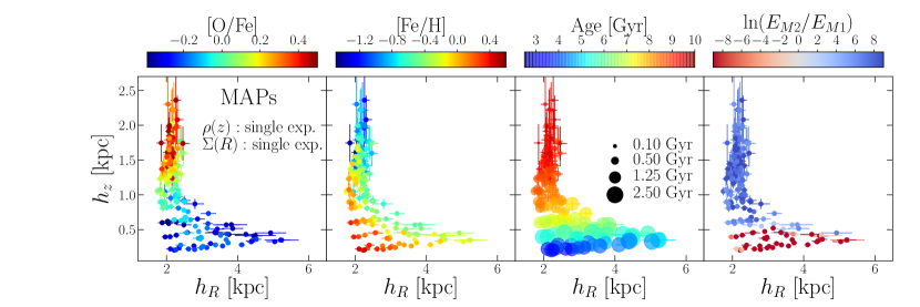
Figure 3: Best fit values of radial scale length $h_{R}$ vs vertical scale height $h_{z}$ for mono-abundance populations of star particles in $5<R<12$ kpc, $0.3<|z|<3$ kpc. From left to right, panels are colour-coded by [O/Fe], [Fe/H], mean age (point sizes meaning age dispersion) and by the Bayes factor comparing the fit quality of single vs double exponentials for the vertical density profile –see Eqs. (9)-(10). In agreement with Bovy et al. (2012), $\alpha$-rich and metal-poor MAPs are thick and centrally concentrated, as opposed to $\alpha$-poor and metal-rich MAPs, which are thin and spread out in radius. MAPs with older stars are more uniform in age and have vertical profiles better fitted by single exponentials, while younger MAPs have broader age distributions and are better fitted by double exponentials.

Fig. 3 shows the best fit values of the scale length $h_{R}$ and scale height $h_{z}$ obtained with model ${\bf M2}$, colour-coded in various ways in the different panels. The first noticeable feature in these plots is the strong anti-correlation between $h_{R}$ and $h_{z}$: the thick populations (high $h_{z}$) are more centrally concentrated (smaller $h_{R}$), while the thinner populations are broadly distributed in radius (large $h_{R}$). The first and second panels are colour-coded by [O/Fe] and [Fe/H], respectively. The thick populations are dominated by stars that are $\alpha$-rich and metal-poor, with a continuous decrease of [O/Fe] and increase of [Fe/H] for the thinner populations. There is also a hint of a radial metallicity gradient, but this is not perfect, with some metal-rich populations being characterized by small $h_{R}$. These results are very similar to those found by Bovy et al. (2012) for the Milky Way. See Fig. 9 and the Appendix for a comparison with the non-clumpy simulation FB80.

The third panel is colour-coded by age, with point sizes representing the age dispersions in each MAP (black points show the scale). The thick and centrally concentrated MAPs are characterized by old stars and are very uniform in age. On the other hand, the thin populations are young on average, but with a much broader age distribution, with age dispersions as large as $2.5$ Gyr.

For a model comparison, we also fit model ${\bf M1}$, i.e. a double exponential for the vertical density profile. The right panel of Fig. 3 is colour-coded by the Bayes factor, Eqs. (9)- (10), comparing models ${\bf M1}$ and ${\bf M2}$ (note that the best fit parameter values shown are still the same as in the other panels, i.e. those of model ${\bf M2}$). While most of the parameter space strongly favours the single exponential (blue points), for some thin disc MAPs the vertical density profile is better described by a double exponential (red points). Comparison with the third panel shows that these are the MAPs with larger age dispersions. Similarly to Minchev et al. (2017), we conclude that in the same manner as the vertical density profile of the complete sample, Fig. 1, seems to be characterized by a double exponential as a consequence of superposing different populations, the double exponentials required for the younger MAPs are also the consequence of mixing different populations (with very different ages).

4.3 Density profiles of mono-age populations

We now analyze the density profiles of co-eval (mono-age) populations defined with 50 bins equally spaced in the logarithm of formation time from 0.1 to 10 Gyr, and selected in a similar region as before ($5<R<12$ kpc), but now including the Galactic plane, i.e. $|z|<3$ kpc, in order to match the selection of Mackereth et al. (2017). We first focus on the vertical density profile of these populations for which, in addition to models ${\bf M1}$ and ${\bf M2}$, Eqs. (4) and (5), we also fit models ${\bf M3}$ and ${\bf M4}$, i.e. a single flaring exponential and a double exponential allowing the inner component to flare, respectively – see Eq. (6) and Table 1.

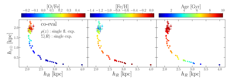
Figure 4: Best fit values of radial scale length $h_{R}$ vs vertical scale height at the Solar position $h_{z\odot}$ for mono-age populations obtained fitting a single flaring exponential model. Star particles are selected in $5<R<12$ kpc, $|z|<3$ kpc. The anti-correlation between $h_{R}$ and $h_{z\odot}$ and the trends with [O/Fe], [Fe/H] and age are similar to, but cleaner than, those for MAPs – Fig. 3.

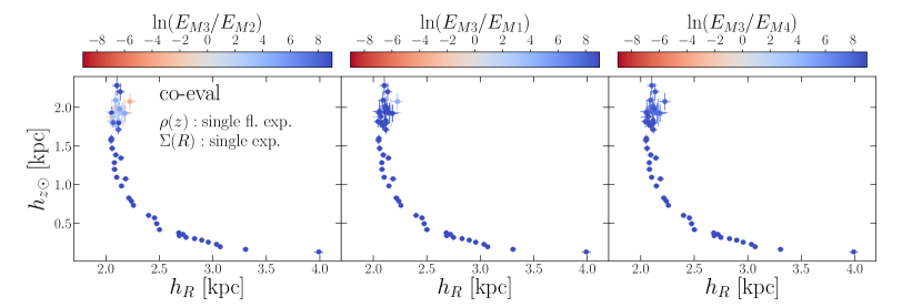
Figure 5: Same as Fig. 4, but now colour-coded by the Bayes factor comparing the fit quality of the flaring single exponential (model M3) with (from left to right) a non-flaring exponential (model M2), a non-flaring double exponential (M1) and a double exponential flaring the thin component (M4). The flaring single exponential is favoured (blue points) in almost all mono-age populations, except for a few thick, old, $\alpha$-rich and metal-poor populations (see Fig. 4), which show weak evidence in favour of a non-flaring single exponential (grey and red points in the left panel).

Fig 4 shows the best fit values of parameters $h_{R}$ and $h_{z\odot}$ obtained with model ${\bf M3}$. The two left panels are again colour-coded by [O/Fe] and [Fe/H] and the third panel is again colour-coded by age. We note an anti-correlation between $h_{R}$ and $h_{z\odot}$ which is similar to, but much clearer than, that of the MAPs in Fig. 3. The thicker (high $h_{z\odot}$) populations are again old, $\alpha$-rich and metal-poor. The metallicity radial gradient is also much more clear than that of the MAPs (middle panel). This clean anti-correlation between scale length and scale height, with the respective trends with abundances and ages, is similar to those found by Stinson et al. (2013) using cosmological simulations. Fig. 10 in the Appendix shows the equivalent results for the non-clumpy simulation FB80, where we conclude that, besides producing the geometric thick disc by converting in-plane to vertical motion, the clumps are also important to increase the radial scale length $h_{R}$ of old, $\alpha$-rich populations due to in-plane scattering – see the Appendix.

The panels in Fig. 5 show the same parameter values as Fig. 4, but now colour-coded by the Bayes factor, Eqs. (9)-(10), comparing the quality of fits of model ${\bf M3}$ (single flaring exponential for the vertical profile) with model ${\bf M2}$ (single non-flaring exponential, left), model ${\bf M1}$ (double non-flaring exponential, middle) and model ${\bf M4}$ (double inner-flaring exponential, right). Model ${\bf M3}$ is strongly favoured with respect to the other models in almost all the co-eval populations (blue points), with a few exceptions for some of the thick populations (high $h_{z\odot}$), which show either a weak evidence in favour of this model or a weak evidence in favour of model ${\bf M2}$ (grey and red points in the left panel).

Having shown that the discs generated by our simulation, and selected by age, generally flare, i.e. get thicker for larger radii, with the vertical density profiles being generally described by single exponentials, we now shift our attention to the radial surface density profiles that, up to this point, were modeled as single exponentials, Eq. (2). An important step in the study of the density profiles of the MW was done by Bovy et al. (2016) who, analyzing red-clump stars from the APOGEE survey, identified that high [$\alpha$/Fe] MAPs have radial surface density profiles well described by single exponentials, while low [$\alpha$/Fe] MAPs show a break in their profiles, with the inner part increasing with radius. Breaks in the radial density profile have been observed also by e.g. Pohlen & Trujillo (2006) in a sample of nearby galaxies from the Sloan Digital Sky Survey (SDSS), by de Jong et al. (2007) in the edge-on galaxy NGC 4244 and by Roškar et al. (2008) in hydrodynamical simulations of self-consistent isolated galaxies – see Debattista et al. (2017). Similar features were later found for both MAPs and mono-age populations in observational and simulation-based results (see e.g. Minchev et al., 2015; Mackereth et al., 2017).

We test these features by means of model ${\bf M5}$, Eq. (7), which is characterized by a broken exponential, i.e. an exponential with slope $h_{R,\mathrm{in}}$ for $R\leq R_{\mathrm{peak}}$ and another exponential with slope $h_{R,\mathrm{out}}$ for $R>R_{\mathrm{peak}}$. Fig. 6 shows the best fit values of the parameters $h_{R,\mathrm{in}}$ and $h_{R,\mathrm{out}}$ versus $h_{z\odot}$. The three left panels are colour-coded as in the previous figures. Note that for the young, $\alpha$-poor and metal-rich populations, the parameters $h_{R,\mathrm{in}}$ and $h_{R,\mathrm{out}}$ assume substantially different values, which already suggests that the data of these populations really require a broken (instead of a single) exponential. Essentially all populations assume positive values for $h_{R,\mathrm{in}}$ (there is only one population for which we found $h_{R,\mathrm{in}}\approx-70$ kpc, whose profile is basically flat in the inner part), which means that, despite the break, their inner profiles are still decreasing functions of radii. Except for the very young, (age $\lesssim 2$ Gyr), all populations approximately have a common $h_{R,\mathrm{out}}\approx 2$ kpc. On the other hand, the parameter $h_{R,\mathrm{in}}$ is anti-correlated with $h_{z\odot}$, similarly to that observed fitting a single exponential (see Fig. 4).

Going up in these panels, i.e. for higher $\alpha$ and age and lower metallicities, the parameter values of $h_{R,\mathrm{in}}$ approach those of $h_{R,\mathrm{out}}$, until they merge into the high-uncertainty region of the $\alpha$-rich, old and metal-poor populations. The right panel compares models ${\bf M5}$ and ${\bf M3}$, i.e. the broken versus single exponential for the surface density $\Sigma(R)$, while keeping a single flaring exponential for $\zeta(z|R)$, Eqs. (5) and  (6). In agreement with the initial suggestion, it is clear that the thicker ($\alpha$-rich and old) populations are better described by single exponentials (red points), while the thinner ones ($\alpha$-poor and younger) are better described by broken exponentials (blue points). This also explains the large uncertainties in $h_{R,\mathrm{in}}$, $h_{R,\mathrm{out}}$ and $h_{z\odot}$ in the thick populations, for which the broken exponential model over-fits the data. See Fig. 11 for a comparison with simulation FB80.

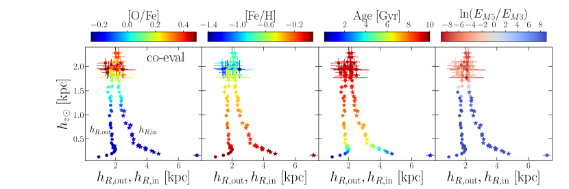
Figure 6: Best fit values of the outer and inner radial scale lengths $h_{R,\mathrm{out}}$, $h_{R,\mathrm{in}}$ vs vertical scale height at the Solar position $h_{z\odot}$ for mono-age populations obtained fitting a single flaring exponential model for $\zeta(z|R)$ and a broken exponential for $\Sigma(R)$ – model M5. The data selection, model fit and colour-coding are the same as that of Fig. 4. Young, $\alpha$-poor and metal-rich populations have sharp breaks, i.e. significant differences $h_{R,\mathrm{in}}-h_{R,\mathrm{out}}$, while old, $\alpha$-rich, metal-poor populations have $h_{R,\mathrm{out}}\approx h_{R,\mathrm{in}}$, and thus flat exponential profiles. The right panel is colour-coded by the Bayes factor comparing the single versus broken exponential models for $\Sigma(R)$. High-[O/Fe] populations are better described by single exponentials (red points), while low [O/Fe] populations strongly favour the broken exponential model (blue points).

Fig. 7 shows the best fit values of the other parameters characterizing the surface density $\Sigma(R)$ as a function of age, obtained with model ${\bf M5}$. The vertical line, approximately at $8.5$ Gyr, divides the samples in low-$\alpha$ (left) and high-$\alpha$ (right) populations, with [O/Fe] abundances lower and larger than zero, respectively. The top panel shows, colour-coded by the Bayes factor, the quantity

$$\Delta=\left[h_{R,\mathrm{out}}^{-1}-h_{R,\mathrm{in}}^{-1}\right]^{-1},$$ (11)

as proposed by Mackereth et al. (2017), and intended to diagnose how sharply broken $\Sigma(R)$ is. A low value of $\Delta$ means a sharp break, while large values mean more broad and continuous profiles (for a single exponential, that quantity tends to infinity). We see that the youngest populations ($\lesssim 2$ Gyr) have sharp breaks, but the profiles get smoother very quickly after $2$ or $3$ Gyr of evolution, with a more gentle smoothing in the later evolution. However, despite this smoothing, a noticeable break is still present for populations as old as $8$ or $9$ Gyr, as indicated by the Bayes factor favouring model ${\bf M5}$ (blue points). This smooth trend is dramatically different for populations older than $9$ Gyr which are better described by single exponentials (red points).

The central panel of Fig. 7 shows the position of the break, $R_{\mathrm{peak}}$, colour-coded by [Fe/H]. $R_{\mathrm{peak}}$ does not depend strongly on age, assuming values between $8$ and $9$ kpc for the $\alpha$-poor populations. For the youngest (age $\lesssim 3$ Gyr) and more metal-rich populations, $R_{\mathrm{peak}}$ decreases for decreasing metallicities. For larger ages, and lower metallicities, $R_{\mathrm{peak}}$ seems to have some wiggles. Since the $\alpha$-rich populations are better described by single exponentials, the uncertainties on $R_{\mathrm{peak}}$ are large, but there is a hint for an increasing $R_{\mathrm{peak}}$ with decreasing metallicities. In their self-consistent hydro-dynamical simulation, Roškar et al. (2008) found a tight correlation between the position of the break and the minimum of the mean age (as a function of radii $R$). In Fig. 8, which shows the mean age as a function of $R$ in our simulation, we observe a minimum at $R\approx 9$ kpc, which is similar to the values of $R_{\mathrm{peak}}$ obtained for the youngest co-eval populations shown in the central panel of Fig. 7.

The bottom panel of Fig. 7 shows the inverse of the typical flaring scale $R_{fl}^{-1}$ colour-coded by [O/Fe]. Small values of $R_{fl}^{-1}$ indicate the absence of a flare, and large values indicate significant flaring. Even for the low-$\alpha$ populations, the dependence on age is not trivial, but we note that the overall $R_{fl}^{-1}$ decreases with age for these populations. For the high-$\alpha$ populations, compatible with the fact that for these populations we have weak or no statistical significance in support of the flaring model (see left panel of Fig. 5), the uncertainties are large, but overall $R_{fl}^{-1}$ seems to increase with age. Fig. 12 in the Appendix shows the equivalent plots for FB80.

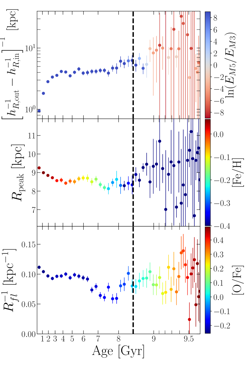
Figure 7: Top: the quantity $\Delta$, Eq. (11), proposed by Mackereth et al. (2017) for measuring how sharply broken $\Sigma(R)$ is (a small value indicates a sharp peak), colour-coded by the Bayes factor comparing a single and a broken exponential models. Center: the position of the break in $\Sigma(R)$, $R_{\mathrm{peak}}$, colour-coded by [Fe/H]. Bottom: inverse flaring radius (a small value means weak flaring), colour-coded by [O/Fe]. The vertical dashed line crosses the bottom panel at [O/Fe]=0 (corresponding to an age $\approx 8.5$ Gyr), defining $\alpha$-poor (left) and $\alpha$-rich (right) regions with very different behavior for all three parameters: low-$\alpha$ populations are described by a broken $\Sigma(R)$, with peak sharpness $\Delta$ decreasing with age, peak position decreasing with age for ages $\lesssim 4$ Gyr and presenting small wiggles for larger ages, and flaring level $R_{fl}^{-1}$ overall decreasing with age. High-$\alpha$ populations have $\Sigma(R)$ better described by single exponentials, thus with large uncertainties for the over-fitting quantities $\Delta$ and $R_{\mathrm{peak}}$. Despite the large uncertainties, $R_{fl}^{-1}$ seems to increase weakly with age for the high-$\alpha$ region.

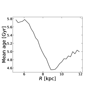
Figure 8: The mean stellar age at each radius obtained with the simulation FB10. As found by Roškar et al. (2008), the position of the minimum, here at $R\approx 9$ kpc, correlates well with the position of the break in $\Sigma(R)$ for the youngest population, shown in the central panel of Fig. 7.

5 Comparison with previous results

We show in Sec. 4.1 that the discs generated by the simulation have gross properties in reasonable agreement with data from the MW (Jurić et al., 2008), and also the expected correlations with age and chemical abundances.

In Sec. 4.2, we showed that when selecting mono-abundance populations and applying geometrical cuts similar to those used by Bovy et al. (2012), we arrive at similar results when fitting single exponentials for both the vertical and radial density profiles: the vertical profile of most of the chemical space is well described by single exponentials, as found by Bovy et al. (2012) – see Fig. 3. The old, $\alpha$-rich and metal poor MAPs are thick and more centrally concentrated, as opposed to the MAPs which are young, $\alpha$-poor and metal-rich, which are thin and radially spread out. The MAPs which are the youngest on average have larger age dispersions and are better described by double exponentials.

Using cosmological simulations and selecting co-eval (mono-age) populations, Stinson et al. (2013) found an anti-correlation between $h_{R}$ and $h_{z}$, and trends with chemical abundances and ages which are similar to, but much cleaner than, those of MAPs. With our isolated galaxy simulation we arrive at very similar results – see Fig. 4.

In a detailed study of nearby galaxies, Comerón et al. (2011) found no evidence for significant flaring of thick discs. Bovy et al. (2016), analyzing red-clump stars from the APOGEE survey, found that the vertical density profiles of thick, $\alpha$-rich MAPs in their sample were described by single non-flaring exponentials, while the thin, $\alpha$-poor MAPs were better described by single flaring exponentials. Minchev et al. (2015), selecting MAPs from cosmological simulations also arrived at a similar conclusion. When selecting co-eval populations, Minchev et al. (2015) found that all populations are described by single flaring exponentials, with a correlation between age and flaring, i.e. that young (old) populations flare less (more).

More recently, Mackereth et al. (2017) using data from the APOGEE survey, analyzed the spatial distribution of red giant stars in the MW. They first split the data into $\alpha$-rich and $\alpha$-poor groups and for each group they selected mono-age, mono-metallicity populations. They also found that all populations are well described by single exponentials with different flaring levels: high-[$\alpha$/Fe] populations tend to flare less in general, with flaring being detected with weaker statistical significance, while low-[$\alpha$/Fe] show a clear, statistically significant flaring. Additionally, Mackereth et al. (2017) found that the $\alpha$-poor populations show an anti-correlation between age and flaring, i.e. that younger (older) populations flare more (less), while for the $\alpha$-rich they found a correlation, i.e. that younger (old) populations flare less (more).

In our analysis, we conclude that the vertical density profiles of old, high-$\alpha$ populations are well described by single exponentials, with weak or no-evidence for flaring, while the low-$\alpha$ populations are well described by single flaring exponentials – see Figs. 4 and 5. The inverse of the flaring radius decreases with age for $\alpha$-poor populations and increases with ages (although with large uncertainties) for $\alpha$-rich populations – see the bottom panel of Fig. 7. All these results are in good agreement with those of Mackereth et al. (2017) for the MW.

Regarding the radial surface density profiles, the $\alpha$-rich co-eval populations are well described by single exponentials, while the $\alpha$-poor populations are better described by broken exponentials, also in agreement with Bovy et al. (2016) and Mackereth et al. (2017). The profiles of younger populations are more sharply broken, and get flatter with age.

A difference between our results and those of Bovy et al. (2016) and Mackereth et al. (2017) is that, despite the breaks, we do not find any population with the inner profile increasing with radius, i.e. with $h_{R,\mathrm{in}}<0$. Another apparent difference is that Mackereth et al. (2017) observe an anti-correlation between the position of the break $R_{\mathrm{peak}}$ and the metallicity, while in our case the trend is the opposite for the younger populations (age $\lesssim 5$ Gyr). On the other hand, we find that overall $R_{\mathrm{peak}}$ changes only by less than 1 kpc for the low-[$\alpha$/Fe] populations and have large uncertainties for the high-[$\alpha$/Fe] populations. However, note that our populations are defined by ages only, i.e. we do not bin in [Fe/H] and thus averaging could be the origin of the observed difference. Another possible explanation for these differences is the fact that the simulated galaxy does not produce a bar, whose contribution to shaping the radial profile might be non-negligible.

Interestingly, running hydrodynamical simulations, Roškar et al. (2008) found that the break of the radial density profile occurs at the same radius for all stellar ages, i.e. that $R_{\mathrm{peak}}$ does not depend on age (the same was observed by de Jong et al. (2007) for NGC 4244). They also found that $R_{\mathrm{peak}}$ coincides with the radius of minimum mean stellar age and that on average $R_{\mathrm{peak}}/h_{R,\mathrm{in}}\approx 2.6$, which is in good agreement with the mean value $2.5$ found by Pohlen & Trujillo (2006) in a sample of nearby galaxies observed by SDSS and the value $2.3\pm 0.7$ found by Elmegreen & Elmegreen (2006) for high-redshift spiral galaxies. Selecting $\alpha$-poor stars (for which the break is present), defined in Fig. 7 as those stars younger than $8.5$ Gyr, we obtain a mean value $R_{\mathrm{peak}}/h_{R,\mathrm{in}}\approx 2.5$. As we can see, the results obtained in this paper are in good agreement with the observational and simulation-based results just mentioned.

Finally, in their (non-clumpy) simulation, Roškar et al. (2008) concluded that the rising mean age in the external disc ($R>R_{\mathrm{peak}}$) is due to radial migration of relatively old stars in nearly circular orbits (for which migration is more efficient). A kinematical analysis of our simulation reveals that approximately $\approx 85\%$ of star particles in the outer disc ($9<R/\mathrm{kpc}<12$) have eccentricity $<0.4$, while $\approx 5\%$ have eccentricity $>0.7$. Thus in our simulation we also conclude that the outer disc is mainly composed of star particles in nearly circular orbits (a significant fraction of which must have migrated from the inner disc), with a small contribution of star particles in highly eccentric orbits generated by early scattering in the clumps.

6 Conclusions

In this paper, we analyze SPH simulations in order to investigate the role of clumps for the evolution of the spatial structure of galactic discs. A simulation with low feedback efficiency allows the formation of clumps which scatter the old stars to high galactic latitudes and sink to the center after $\approx 4$ Gyr. We show that this simulation naturally gives rise to galactic discs (particularly a thick disc) with properties in good agreement with those observed in the Milky Way.

Selecting all stars in a given geometric cut, without any additional cut in chemistry or age, the vertical density profile is characterized by the typical double exponential law, with the same trends observed in the Milky Way (Bensby et al., 2005; Jurić et al., 2008): the geometric thick disc is composed of stars that are old, rich in [$\alpha$/Fe] and metal poor, while the thin disc is dominated by stars that are young, [$\alpha$/Fe]-poor and metal-rich.

Applying chemical cuts, we observe that mono-abundance populations are generally characterized by single exponential vertical density profiles, with the exception of some young MAPs with large age dispersions, which require a double exponential.

The selection of mono-age populations results in vertical density profiles well described by single exponentials with very clean correlations between the vertical scale height $h_{z}$ and radial scale length $h_{R}$, as observed by Stinson et al. (2013). The radial density profiles of high-$\alpha$ mono-age populations are also single exponentials, while those of low-$\alpha$ populations are broken exponentials. The sharpness of the break decreases with age, which is probably the consequence of radial migration erasing primeval gradients, as pointed out by Mackereth et al. (2017).

It is interesting to note that radial migration is also traditionally believed to be responsible for the flaring of low [$\alpha$/Fe] populations, i.e. for the disc thickening at larger radii for the stars in the geometric thin disc, in which case one would expect young populations to flare less. However, we find (in agreement with Mackereth et al., 2017) the opposite trend, i.e. that the flaring level, $R_{fl}^{-1}$, decreases with age for these populations – see Fig. 7. This fact is interpreted by Mackereth et al. (2017) as suggestive that old mergers have suppressed the flaring of the old populations in the Milky Way. On the other hand, since we simulate an isolated galaxy, our results show that internal dynamical processes are able to build the observed trends, without the need for mergers.

The detailed agreement of the results presented in this work with various observational results allows us to conclude that the scattering of old, $\alpha$-rich and metal-poor stars by clumps formed early in the Galaxy is a viable mechanism for the formation of the thick disc.

Appendix A Comparison with a non-clumpy simulation

In this section, we perform the same analysis as that of Sec. 4, but applied to the simulation FB80, in which the stellar feedback efficiency is set to $80\%$. As discussed in Sec. 2, this high feedback efficiency inhibits the formation of clumps and thus the comparison of results from simulations FB10 and FB80 allows us to clarify the role of the clumps. We already showed in Fig. 2 that the vertical density profile obtained with the simulation FB80 is characterized by a single exponential, i.e. that this simulation does not produce a geometric thick disc.

In Fig. 9, we show the best fit values of the scale length $h_{R}$ and scale height $h_{z}$ obtained fitting single exponentials, Eqs. (2) and (5), to mono-abundance populations (MAPs) selected from the simulation FB80. This figure is to be compared to Fig. 3. First, we note that the typical values of $h_{z}$ are significantly smaller than those in Fig. 3, showing again the absence of thicker components in FB80. Additionally, the anti-correlation between $h_{z}$ and $h_{R}$ observed for the simulation FB10 and for the Milky Way (Bovy et al., 2012) is blurred for FB80, with the best fit parameter values being more spread in the diagram.

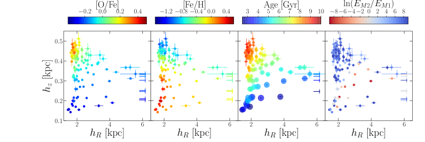
Figure 9: Best fit values of radial scale length $h_{R}$ vs vertical scale height $h_{z}$ for mono-abundance populations of star particles in $5<R<12$ kpc, $0.3<|z|<3$ kpc in the simulation FB80. From left to right, panels are colour-coded by [O/Fe], [Fe/H], mean age (point sizes meaning age dispersion) and by the Bayes factor comparing the fit quality of single vs double exponentials for the vertical density profile –see Eqs. (9)-(10). The anti-correlation between $h_{R}$ and $h_{z}$ observed in the simulation FB10 – Fig. 3 – and in the MW (Bovy et al., 2012) is blurred here. Note also that the vertical scale is smaller than that of Fig. 3.

Fig. 10 (to be compared to Fig. 4), shows the best fit values of the scale length $h_{R}$ and scale height at the Solar position $h_{z\odot}$ obtained fitting the single flaring exponential model, Eqs. (2), (5) and (6), to the data of simulation FB80. The main difference with respect to Fig. 4 is again the typical values of $h_{z\odot}$, which are significantly smaller for FB80. It is interesting to note also that the thicker and older components in FB80 assume $h_{R}$ values significantly smaller than those in FB10 (Fig. 4). A possible interpretation for this is the following: in the clumpy simulation FB10, the old, $\alpha$-rich populations are scattered by the clumps. In the reference frame of the clump, this scatter is quasi-isotropic, i.e. scatters to any direction are equally probable. Since the clumps are moving in the galactic plane, in the reference frame of the galactic center this scattering should have some anisotropy but, still, scatters that promote stars to high latitudes $z$ also tend to increase the dispersion of radii $R$. In this way, the absence of scattering in FB80, apart from not allowing the formation of thicker components, also does not allow the promotion of the older stars, typically formed in inner radii (inside-out growth) to larger radii. The direct consequence is that in the non-clumpy simulation the scale lengths $h_{R}$ of old populations are only affected by secular heating and are closer to their pristine values and thus typically small. On the other hand, the youngest and thinnest populations are not affected by the clumps, which have sunk to the center by $\approx 4$ Gyr in FB10. In this way, the typical values of $h_{R}$ and $h_{z}$ for these populations are similar in the two simulations.

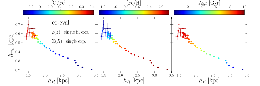
Figure 10: Best fit values of radial scale length $h_{R}$ vs vertical scale height at the Solar position $h_{z\odot}$ for mono-age populations obtained fitting a single flaring exponential model for the simulation FB80. Star particles are selected in $5<R<12$ kpc, $|z|<3$ kpc. The anti-correlation between $h_{R}$ and $h_{z\odot}$ in this case is different from that observed in the simulation FB10 – Fig. 4 – and by Stinson et al. (2013) in cosmological simulations, with $\alpha$-rich populations assuming smaller values for both $h_{z\odot}$ and $h_{R}$.

Fig. 11, to be compared to Fig. 6, shows the best fit values of $h_{R,\mathrm{in}}$ and $h_{R,\mathrm{out}}$ obtained fitting the broken exponential model to the radial profiles of co-eval populations in the simulation FB80. Once more, the scale height and scale length of old populations are typically small in comparison to the clumpy simulation FB10. On the other hand, young populations have similar parameter values in both simulations.

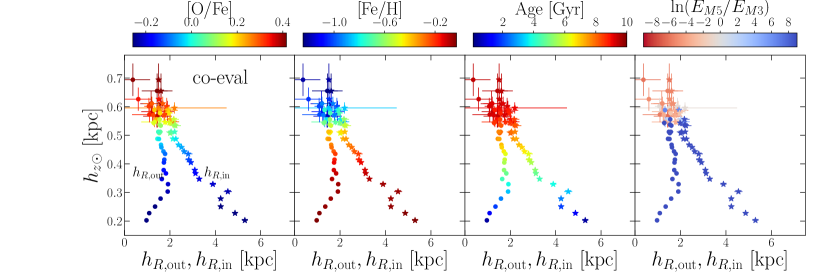
Figure 11: Best fit values of the outer and inner radial scale lengths $h_{R,\mathrm{out}}$, $h_{R,\mathrm{in}}$ vs vertical scale height at the Solar position $h_{z\odot}$ for mono-age populations obtained fitting a single flaring exponential model for $\zeta(z|R)$ and a broken exponential for $\Sigma(R)$ – model M5 to the simulation FB80. The data selection, model fit and colour-coding are the same as that of Fig. 4. The small values of $h_{z\odot}$, in comparison to Fig. 6, indicate the absence of a thick disc. Young, $\alpha$-poor and metal-rich populations have sharp breaks, i.e. significant differences ${h_{R,\mathrm{in}}-h_{R,\mathrm{out}}}$, while old, $\alpha$-rich, metal-poor populations have $h_{R,\mathrm{out}}\approx h_{R,\mathrm{in}}$, and thus flat exponential profiles. The right panel is colour-coded by the Bayes factor comparing the single versus broken exponential models for $\Sigma(R)$. High-[O/Fe] populations are better described by single exponentials (red points), while low [O/Fe] populations strongly favour the broken exponential model (blue points).

Fig. 12 shows, as a function of age, the quantities characterizing the break in the radial profiles and the flaring of the vertical profiles produced by the simulation FB80, and is to be compared to Fig. 7 produced by the simulation FB10. Here, the vertical line defining low and high-$\alpha$ regions ([O/Fe] $\lessgtr 0$) is at $\approx 7.5$ Gyr. Overall these plots are similar to those for FB10, particularly, in the top panel, the quantity $\Delta$, Eq. (11), measuring how sharp is the break: young populations have sharp breaks, but 2 or 3 Gyrs of radial migration (produced by the spiral arms and equally present in the two simulations) flattens the radial profiles. In the middle panel, we see that the position of the break seems to vary more with age ($\approx 2.5$ Gyr) in FB80, but this variation is still smaller than those reported by Mackereth et al. (2017) for the Milky Way. Finally, the bottom panel shows that in FB80 the young, $\alpha$-poor populations seem to flare more than in FB10.

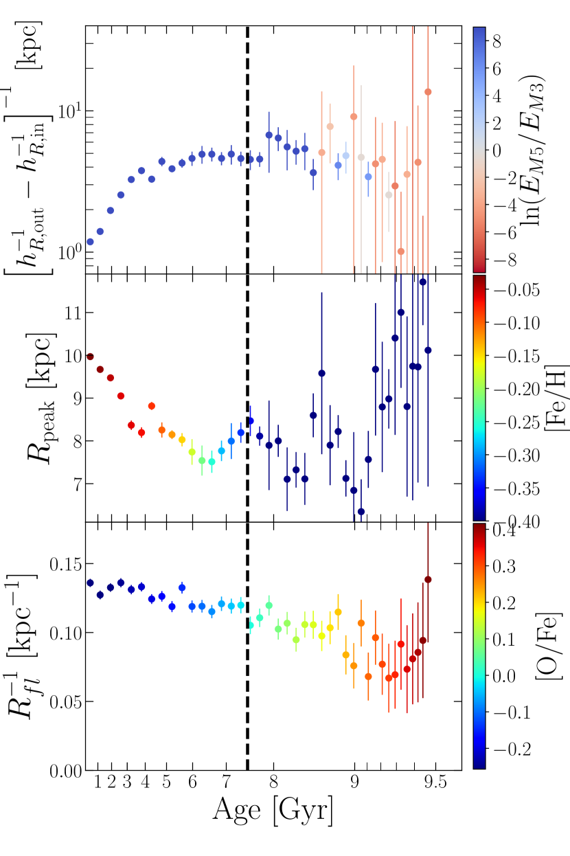
Figure 12: The same quantities shown in Fig. 7, but now for the non-clumpy simulation FB80. The vertical dashed line crosses the bottom panel at [O/Fe]=0 (corresponding now to an age $\approx 7.5$ Gyr): low-$\alpha$ populations are again described by a broken $\Sigma(R)$, with peak sharpness $\Delta$ decreasing with age, peak position decreasing with age for ages $\lesssim 4$ Gyr and presenting some wiggles for larger ages, and flaring level $R_{fl}^{-1}$ generally larger than in FB10. High-$\alpha$ populations have $\Sigma(R)$ better described by single exponentials, thus with large uncertainties for the over-fitting quantities $\Delta$ and $R_{\mathrm{peak}}$.

References

- Agertz et al. (2009) Agertz O., Teyssier R., Moore B., 2009, MNRAS, 397, L64
- Anders et al. (2014) Anders F., et al., 2014, AAP, 564, A115
- Belokurov et al. (2018) Belokurov V., Erkal D., Evans N. W., Koposov S. E., Deason A. J., 2018, MNRAS, 478, 611
- Bensby et al. (2005) Bensby T., Feltzing S., Lundström I., Ilyin I., 2005, AAP, 433, 185
- Bournaud et al. (2009) Bournaud F., Elmegreen B. G., Martig M., 2009, ApJL, 707, L1
- Bovy et al. (2012) Bovy J., Rix H.-W., Liu C., Hogg D. W., Beers T. C., Lee Y. S., 2012, ApJ, 753, 148
- Bovy et al. (2016) Bovy J., Rix H.-W., Schlafly E. F., Nidever D. L., Holtzman J. A., Shetrone M., Beers T. C., 2016, ApJ, 823, 30
- Buck (2020) Buck T., 2020, MNRAS, 491, 5435
- Buck et al. (2017) Buck T., Macciò A. V., Obreja A., Dutton A. A., Domínguez-Tenreiro R., Granato G. L., 2017, MNRAS, 468, 3628
- Bullock et al. (2001) Bullock J. S., Dekel A., Kolatt T. S., Kravtsov A. V., Klypin A. A., Porciani C., Primack J. R., 2001, ApJ, 555, 240
- Burstein (1979) Burstein D., 1979, ApJ, 234, 829
- Clarke et al. (2019) Clarke A. J., et al., 2019, MNRAS, 484, 3476
- Comerón et al. (2011) Comerón S., et al., 2011, ApJ, 741, 28
- Comerón et al. (2014) Comerón S., Elmegreen B. G., Salo H., Laurikainen E., Holwerda B. W., Knapen J. H., 2014, AAP, 571, A58
- Debattista et al. (2017) Debattista V. P., Roškar R., Loebman S. R., 2017, in Knapen J. H., Lee J. C., Gil de Paz A., eds, Astrophysics and Space Science Library Vol. 434, Outskirts of Galaxies. p. 77 (arXiv:1706.01996), doi:10.1007/978-3-319-56570-5_3
- Elmegreen & Elmegreen (2006) Elmegreen B. G., Elmegreen D. M., 2006, ApJ, 650, 644
- Elmegreen et al. (2017) Elmegreen B. G., Elmegreen D. M., Tompkins B., Jenks L. G., 2017, ApJ, 847, 14
- Foreman-Mackey et al. (2013) Foreman-Mackey D., Hogg D. W., Lang D., Goodman J., 2013, PASP, 125, 306
- Genel et al. (2012) Genel S., et al., 2012, ApJ, 745, 11
- Gilmore & Reid (1983) Gilmore G., Reid N., 1983, MNRAS, 202, 1025
- Hayden et al. (2015) Hayden M. R., et al., 2015, ApJ, 808, 132
- Helmi et al. (2018) Helmi A., Babusiaux C., Koppelman H. H., Massari D., Veljanoski J., Brown A. G. A., 2018, Nature, 563, 85
- Hopkins et al. (2012) Hopkins P. F., Kereš D., Murray N., Quataert E., Hernquist L., 2012, MNRAS, 427, 968
- Ivezić et al. (2014) Ivezić Ž., Connelly A. J., VanderPlas J. T., Gray A., 2014, Statistics, Data Mining, and Machine Learning in Astronomy
- Jurić et al. (2008) Jurić M., et al., 2008, ApJ, 673, 864
- Kass & Raftery (1995) Kass R. E., Raftery A. E., 1995, Journal of the American Statistical Association, 90, 773
- Loebman et al. (2011) Loebman S. R., Roškar R., Debattista V. P., Ivezić Ž., Quinn T. R., Wadsley J., 2011, ApJ, 737, 8
- Loebman et al. (2016) Loebman S. R., Debattista V. P., Nidever D. L., Hayden M. R., Holtzman J. A., Clarke A. J., Roškar R., Valluri M., 2016, ApJL, 818, L6
- Mackereth et al. (2017) Mackereth J. T., et al., 2017, MNRAS, 471, 3057
- Mackereth et al. (2018) Mackereth J. T., Crain R. A., Schiavon R. P., Schaye J., Theuns T., Schaller M., 2018, MNRAS, 477, 5072
- Minchev et al. (2015) Minchev I., Martig M., Streich D., Scannapieco C., de Jong R. S., Steinmetz M., 2015, ApJ, 804, L9
- Minchev et al. (2017) Minchev I., Steinmetz M., Chiappini C., Martig M., Anders F., Matijevic G., de Jong R. S., 2017, ApJ, 834, 27
- Navarro et al. (1997) Navarro J. F., Frenk C. S., White S. D. M., 1997, ApJ, 490, 493
- Nelder & Mead (1965) Nelder J. A., Mead R., 1965, The Computer Journal, 7, 308
- Nidever et al. (2014) Nidever D. L., et al., 2014, ApJ, 796, 38
- Oklopčić et al. (2017) Oklopčić A., Hopkins P. F., Feldmann R., Kereš D., Faucher-Giguère C.-A., Murray N., 2017, MNRAS, 465, 952
- Pilkington et al. (2012) Pilkington K., et al., 2012, MNRAS, 425, 969
- Pohlen & Trujillo (2006) Pohlen M., Trujillo I., 2006, AAP, 454, 759
- Roškar et al. (2008) Roškar R., Debattista V. P., Stinson G. S., Quinn T. R., Kaufmann T., Wadsley J., 2008, ApJL, 675, L65
- Schönrich & Binney (2009) Schönrich R., Binney J., 2009, MNRAS, 399, 1145
- Shen et al. (2010) Shen S., Wadsley J., Stinson G., 2010, MNRAS, 407, 1581
- Spitzer & Schwarzschild (1953) Spitzer Jr. L., Schwarzschild M., 1953, ApJ, 118, 106
- Stinson et al. (2006) Stinson G., Seth A., Katz N., Wadsley J., Governato F., Quinn T., 2006, MNRAS, 373, 1074
- Stinson et al. (2013) Stinson G. S., et al., 2013, MNRAS, 436, 625
- Tsikoudi (1979) Tsikoudi V., 1979, ApJ, 234, 842
- Wadsley et al. (2004) Wadsley J. W., Stadel J., Quinn T., 2004, NA, 9, 137
- Yoachim & Dalcanton (2006) Yoachim P., Dalcanton J. J., 2006, AJ, 131, 226
- Yoachim & Dalcanton (2008a) Yoachim P., Dalcanton J. J., 2008a, ApJ, 682, 1004
- Yoachim & Dalcanton (2008b) Yoachim P., Dalcanton J. J., 2008b, ApJ, 683, 707
- Yoshii (1982) Yoshii Y., 1982, PASJ, 34, 365
- de Jong et al. (2007) de Jong R. S., et al., 2007, ApJL, 667, L49