Numerical conformal mapping with rational functions

Abstract

New algorithms are presented for numerical conformal mapping based on rational approximations and the solution of Dirichlet problems by least-squares fitting on the boundary. The methods are targeted at regions with corners, where the Dirichlet problem is solved by the “lightning Laplace solver” with poles exponentially clustered near each singularity. For polygons and circular polygons, further simplifications are possible.

1 Introduction

The association of conformal mapping with Laplace problems goes back to the beginning of the subject henrici ; schiffer . When this connection has been exploited for the numerical computation of conformal maps, it has usually been by way of integral equations such as those of Berrut, Gerschgorin, Lichtenstein, Symm, and Warschawski gaier ; henrici ; tref ; wegmann . However, almost all domains of interest in practical conformal mapping contain corners, and for such domains, it has recently been discovered that rational functions with exponentially clustered poles offer a powerful alternative approach to solving Laplace problems lightning . The aim of this paper is to bring these ideas together to present simple new algorithms for numerical conformal mapping. A second, different aspect of rational functions introduced in gt also comes into play: the compression of a computed conformal map to a more compact form by means of the AAA algorithm AAA ; lawson .

As shown in lightning , rational functions can achieve root-exponential convergence for almost arbitrary corner singularities, i.e., $O(C^{\kern 0.5pt-\sqrt{n}}\kern 0.4pt)$ as a function of the rational degree $n$ for a constant $C>1$, and no analysis of the singularities is needed. This means that our method does not care if the boundary components are straight or curved, so long as they are smooth. Unbounded domains are also not a problem.

For simply-connected domains with smooth boundaries, the idea of conformal mapping via Laplace problems can be realized by means of polynomials instead of rational functions, and we begin in Section 2 by presenting an algorithm of this kind. Though this method is sometimes effective, it often fails for reasons related to the “crowding phenomenon” of numerical conformal mapping. Methods based on integral equations are superior, and such a method is the default used in the new Chebfun code conformal. The picture changes sharply when we turn to rational functions in Section 3. We show that a conformal map of a simply-connected domain with corners can be computed in a few lines of code by calling the MATLAB “lightning Laplace solver” laplace lightcode .

Both the polynomial and rational function methods are readily generalized to doubly connected domains, and these generalizations are presented for smooth boundaries in Section 4 and for boundaries with corners in Section 5. Domains of higher connectivity are considered in Section 6, and numerical details of our methods are discussed in Section 7. Section 8 discusses the further simplifications available for polygons and circular polygons if one uses a modified method based on explicit information about corner singularities. Conclusions are presented in Section 9.

2 Smooth simply connected domains

Let $\Omega\in{\bf C}$ be a simply connected domain bounded by a Jordan curve $P$, and let $D$ and $S$ be the open unit disk and the unit circle. Without loss of generality we assume $0\in\Omega$ and seek the unique conformal map $f:\Omega\mapsto D$ such that $f(0)=0$ and $f^{\prime}(0)>0$. By the Osgood–Carathéodory theorem henrici , $f$ extends to a homeomorphism of $\overline{\Omega}$ onto $\overline{D}$. It follows that $g(z)=\log(f(z)/z)$ is a nonzero analytic function on $\Omega$ that is continuous on $\overline{\Omega}$ and has real part $-\log|z|$ for $z\in P$ and imaginary part $0$ at $z=0$. If we write $g$ as $g(z)=u(z)+iv(z)$, where $u$ and $v$ are real harmonic functions in $\Omega$, continuous on $\overline{\Omega}$, then $u$ is the unique solution of the Dirichlet problem

$$\Delta u=0\,;\quad u(z)=-\log|z|,~{}z\in P,$$ (1)

and $v$ is its unique harmonic conjugate in $\Omega$ with $v(0)=0$. Combining these elements, we see that $f$ takes the form

$$f(z)=ze^{u(z)+iv(z)}.$$ (2)

Note that $u(z)+\log|z|$ is the Green’s function of $\Omega$ with respect to the point $z=0$, so $f$ is nothing more than the exponential of the analytic extension of the Green’s function. See (henrici, , Thm. 16.5a) and (schiffer, , p. 253).

To compute the conformal map $f$, therefore, it is enough to solve the Dirichlet problem (1) for $u$ and then find its harmonic conjugate $v$. In this paper we approximate solutions to Dirichlet problems by the real parts of analytic functions defined by series involving polynomials, rational functions, or other elementary terms. The harmonic conjugates come for free from the same expansion coefficients.

In this section we consider the simplest case, in which $P$ is well-behaved enough that it is effective to work with polynomials. We first outline the algorithm in the monomial basis and then mention the variation involving Arnoldi factorization that our codes actually employ. Following series , let $u$ be approximated as

$$u(z)\approx\kern 0.7pt\hbox{Re}\kern 0.7pt\kern-1.0pt\sum_{k=0}^{n}c_{k}z^{k}$$ (3)

for some degree $n$ and complex coefficients $c_{k}$, which will depend on $n$. Writing $c_{k}=a_{k}+ib_{k}$, we have

$$u(z)\approx\sum_{k=0}^{n}\,\bigl{(}a_{k}\kern 0.7pt\hbox{Re}\kern 0.7pt(z^{k})-b_{k}\kern 0.7pt\hbox{Im}\kern 0.7pt(z^{k})\bigr{)}.$$ (4)

With $b_{0}=0$, this gives us $N=2n+1$ real unknowns $a_{0},\dots,a_{n}$ and $b_{1},\dots,b_{n}$. These are determined numerically by sampling the function $-\log|z|$ in $M\gg N$ points on $P$ and solving an $M\times N$ matrix least-squares problem of the form $Ax\approx b$; we take $M\approx 4N$. The harmonic conjugate is then approximated by the series

$$v(z)\approx\sum_{k=0}^{n}\,\bigl{(}a_{k}\kern 0.7pt\hbox{Im}\kern 0.7pt(z^{k})+b_{k}\kern 0.7pt\hbox{Re}\kern 0.7pt(z^{k})\bigr{)},$$ (5)

and $f$ comes from (2). Note that if $P$ is analytic, then $f$ can be analytically continued to a neighborhood of $\overline{\Omega}$, and geometric convergence of (4) and (5) is guaranteed (in exact arithmetic) as $n\to\infty$ walsh , assuming the boundary sampling is fine enough that the discrete least-squares problem on $P$ approximates the continuous one. (There are also special cases in which $P$ is not smooth and yet $f$ is still analytic everywhere on $P$, such as a rectangle, an equilateral triangle, or the “circular L-shape” consisting of a square from which a quarter-circular bite has been removed.)

By the method just described, if $\Omega$ is well enough behaved, one can compute a polynomial-based approximation of the conformal map $f$. The degree $n$ will usually have to be high. However, as described in gt , the computed map can be compressed to a much more compact form as a rational function by means of the AAA approximation algorithm AAA . Moreover, the AAA method can be invoked a second time to compute a rational approximation of the inverse map $f^{-1}$. As emphasized in gt , when AAA approximation is brought into play, the traditional fundamental difference between conformal maps in the forward and inverse directions ceases to be very important. Once one is available, the other is readily computed too.

The presentation of the last page has been framed with respect to monomial bases $1,z,z^{2},\dots.$ Unless $P$ is close to a circle about the origin, however, the monomials will be very ill-conditioned, and it is better to use an approximation to a family of polynomials orthogonal over $P$. This we do by carrying out an Arnoldi iteration as described in VmeetsA . Mathematically the two approaches are equivalent.

We summarize the algorithm, which we call Algorithm P1 (P for polynomial, 1 for simply connected), as follows. This is a high-level description, omitting many details, and the parameters indicated are engineering choices, not claimed to be optimal. For reasons discussed in gt , high accuracy tends to be problematic in numerical conformal mapping, and we work by default to a tolerance of $10^{-5}$.

Algorithm P1.

$\bullet$ For $n=$ rounded values of $2^{4},2^{4.5},2^{5},\dots$ until convergence or failure,

- Set $M=8\kern 0.3ptn$ and sample ${-}\kern 1.0pt\log|z|$ in $M$ points of $P$;

- Solve an $M\times N$ least-squares problem for the approximation $(\ref{approx})$;

- For stability, do this via Arnoldi factorization as described in VmeetsA .

$\bullet$ Form $v$ from $(\ref{vapprox})$ and $f$ from $(\ref{frep})$;

$\bullet$ Approximate $f$ by a AAA rational approximation;

$\bullet$ Approximate $f^{-1}$ by another AAA rational approximation.

This algorithm is available in Chebfun chebfun in the command conformal, introduced in October, 2019, if it is called with the flag ’poly’. It is not the default algorithm used by conformal, as we shall explain in a moment.

Figure 1 illustrates Algorithm P1 applied to a smooth domain with five-fold symmetry, showing the output from the Chebfun commands

     C = chebfun(’exp(1i*pi*t)*(1+.15*cos(5*pi*t))’, ’trig’);
     [f, finv] = conformal(C, ’poly’, ’plots’);

The objects f and finv are function handles corresponding to rational approximations of degrees 26 and 22, respectively, of the functions $f$ and $f^{-1}$. These degrees are remarkably low. The computation takes about $0.3$ seconds on a desktop machine, plus another second for plotting, and the maximal error on the boundary is about $10^{-5}$.

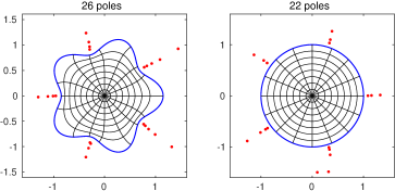
Figure 1: Conformal map of a smooth domain computed to about $5$-digit accuracy in $0.2$ seconds on a desktop machine by Algorithm P1 via the Chebfun conformal(...,’poly’) command. The red dots mark poles of the rational representations of $f$ and $f^{-1}$: just $26$ poles for $f$ and $22$ for $f^{-1}$. The closest poles lie at distance $0.099$ from $P$ on the left and at distance $0.059$ from $S$ on the right.

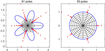
Figure 2: If the lobes are made deeper by changing the coefficient of the cosine term from $0.15$ to $0.5$, Algorithm P1 fails because it would require a polynomial of degree in the tens of thousands. Instead this figure was computed via the Kerzman–Stein integral equation, the default algorithm of Chebfun conformal. The closest poles now lie at distances $0.013$ from $P$ on the left and $0.0011$ from $S$ on the right. The AAA rational representations are still remarkably economical.

All this sounds good, but in fact, Algorithm P1 is limited in its capabilities, and will fail for many smooth domains. For example, it fails if the indentations in the domain of Figure 1 are made twice as deep by changing the coefficient $0.15$ to $0.30$. The problem in such a case is that the polynomial degree would have to be in the thousands, a consequence of the large distortions in conformal mapping that go by the name of the crowding phenomenon wegmann . If $0.30$ is increased further to $0.50$, we get the domain shown in Figure 2, and this was certainly not mapped with Algorithm P1. The default method of conformal was applied instead, involving a discretization of the Kerzman–Stein integral equation ks ; kt followed by AAA rational compression in both directions. For this domain, Algorithm P1 would require a polynomial of degree in the tens of thousands.

There is a literature on the crowding phenomenon, and in particular, see Theorems 2–5 of gt . These establish that if $\Omega$ contains an outward-pointing finger of length-to-width ratio $L$ as defined in a certain precise sense, then $f^{-1}$ must be at least as large as order $e^{\pi L}$ at some points of $S$, with singularities (or at least points of non-univalency) at distances no greater than order $e^{-\pi L}$ from $S$, and that any useful polynomial approximation $p\approx f^{-1}$ must have degree at least on the order of $e^{\pi L}$. (In Figure 2 we have $L\approx 1.75$ and $e^{\pi L}\approx 244$.) Analogous if somewhat weaker effects occur for $f$ and its polynomial approximations if there are inward-pointing fingers. The geometric convergence mentioned earlier still applies, but is useless in practice because the constant $C$ exceeds $1$ by only a small amount. These effects are reflected in the positions of the red dots marking poles in Figures 1 and 2, highlighting the profound difference between polynomial and rational approximations. In the right image of each pair, the poles cluster near points of $S$ that map to outward-pointing lobes of $\Omega$. Similarly, the poles in the left image cluster near points of $P$ at inward-pointing fingers.

We emphasize that the effects just discussed will cause trouble for any method based on polynomial approximations, no matter how stably implemented, for they have nothing to do with the choice of polynomial basis. Our Arnoldi factorization makes the implementation quite stable, but still it will fail for domains whose maps involve large distortions.

Variants of Algorithm P1 can be used to solve related problems involving exterior domains. To map the interior of $P$ to the exterior of $S$, we change the factor $z$ to $z^{-1}$ in (2); the Dirichlet problem (1) remains unchanged. To map the exterior of $P$ to the exterior of $S$, we replace positive by negative powers in (3)–(5). To map the exterior of $P$ to the interior of $S$, we make both of these changes.

We now turn now to the much more powerful Algorithm R1 based on rational functions.

3 Simply connected domains with corners

Let the boundary $P$ of $\Omega$ be a polygon or circular polygon or other Jordan curve consisting of a finite set of analytic curves meeting at corners $z_{1},\dots,z_{K}$. (A circular polygon is a finite chain of circular arcs.) As before, we assume $0\in\Omega$ and seek the conformal map $f:\Omega\mapsto D$ with $f(0)=0$ and $f^{\prime}(0)>0$.

Equations (1) and (2) still hold: we need to solve a Dirichlet problem, but now, there will be singularities at the corners. Instead of (3), we consider

$$u(z)\approx\kern 0.7pt\hbox{Re}\kern 0.7pt\Biggl{[}\;\sum_{j=1}^{n_{1}}{a_{j}\over z-z_{j}}\;+\;\sum_{j=0}^{n_{2}}b_{j}z^{j}\Biggr{]}$$ (6)

with complex coefficients $a_{j}$ and $b_{j}$; again, the polynomial part of the sum will be implemented in practice by an Arnoldi factorization VmeetsA . Since the publication of a paper by Newman in 1964 newman , it has been recognized that rational functions of the form of the first sum in brackets can approximate certain singularities with root-exponential convergence, if the poles $z_{j}$ are clustered exponentially near the singular points with a spacing that scales with $n_{1}^{-1/2}$. In lightning it was proved that this effect applies generally to solutions of Lapalce Dirichlet problems defined by piecewise analytic functions meeting at corners. In particular, Theorem 2.3 of lightning implies that approximations of the form (6) can converge root-exponentially for the conformal map $f$. (The proof given in lightning assumes $P$ is convex, but it is believed that the result holds generally.) Since the appearance of lightning , a MATLAB “lightning Laplace solver” code laplace has been developed to solve Dirichlet problems by this method lightcode .

We summarize our algorithm, Algorithm R1.

Algorithm R1.

$\bullet$ Solve problem $(\ref{dirichlet})$ by the lightning method and form $f$ from (2);

$\bullet$ Approximate $f$ by a AAA rational approximation;

$\bullet$ Approximate $f^{-1}$ by another AAA rational approximation.

Using laplace, all this can be done in four lines of MATLAB, assuming a specification of $P$ and a tolerance tol have been given. If $P$ is just a polygon, then P can be just a vector of vertices. By default we take $\hbox{\tt tol}=10^{-6}$:

     [~, ~, w, Z] = laplace(P, @(z) -log(abs(z)), ’tol’, tol);
     W = Z.*exp(w(Z));
     f = aaa(W, Z, ’tol’, tol);
     finv = aaa(Z, W, ’tol’, tol);

This is the central message of this paper: the conformal map of a domain with corners can be computed in this simple fashion. Section 7 will discuss certain numerical details.

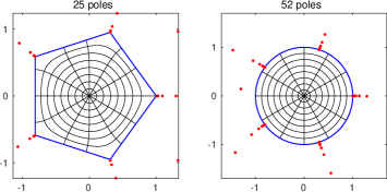
Figure 3: Conformal map of a pentagon computed in about $0.3$ secs. by Algorithm R1.

Figure 3 illustrates Algorithm R1 applied to a regular pentagon, a polygonal analogue of the domain of Figure 1. Five-digit accuracy is achieved in about $0.3$ secs. of desktop time, with poles in both directions clustering near the five singular points. There are four poles near the vertex at $z=1$, for example, whose distances from the vertex are approximately

     0.0097,  0.044,  0.14,  0.49.

Though these poles were chosen adaptively by the AAA algorithm, based on no mathematical analysis, they show exponential clustering with a ratio of successive distances on the order of $3$.

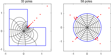
Figure 4: Mapping of an L-shaped domain by Algorithm R1. The map $f$ is nonsingular at the salient corners, so on the left, poles cluster only at the reentrant corner, whereas on the right they cluster at six points.

Figure 5: The rational approximations produced by Algorithm R1 can be evaluated in just microseconds. This figure shows images under $f^{-1}$ of 10,000 uniformly distributed random points in the unit disk, computed in about $0.005$ secs. total. The nonuniform shading illustrates the exponential distortion effects in conformal maps, discussed in Section $2$.

Figure 4 shows results of an analogous computation, taking about half a second, for an L-shaped domain. On the left, poles cluster near the reentrant corner at distances approximately

    0.000053, 0.00030, 0.00069, 0.0071, 0.0013, 0.0022, 0.0035,
    0.0054, 0.081, 0.012, 0.017, 0.024, 0.034, 0.047, 0.066,
    0.091, 0.12, 0.17, 0.23, 0.31, 0.42, 0.56, 0.76, 1.04, 1.66.

These show exponential spacing with a factor of about 1.4. The reduction of the factor from 3 to 1.4 as the number of poles near a corner increases from 4 to 25 is consistent with root-exponential clustering theorems of lightning .

We emphasize the extraordinary economy of the representations of conformal maps computed by Algorithm R1, since they are nothing more than rational functions of a degree typically less than 100.  Figure 5 shows images of $10^{4}$ points in the unit disk, computed in $0.005$ secs. all together.

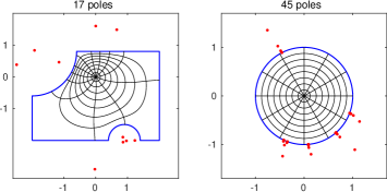
Figure 6: Conformal map of a circular polygon computed by Algorithm R1. This shape is the first example presented by Howell in howell .

Figure 7: Another map of a circular polygon computed by Algorithm R1. Each boundary component is a circular arc of radius $2$.

These examples involve polygons, but Algorithm R1 is equally applicable to other domains bounded by analytic arcs meeting at corners. For example, a circular polygon is a generalization of a polygon in which each side may be a straight segment or a circular arc. Whereas polygons are conventionally mapped by the Schwarz–Christoffel integral, circular polygons can be mapped by the so-called Schwarzian differential equation SCbook . This idea goes goes back to Schwarz himself 150 years ago, but has rarely been attempted numerically; the two realizations we know of are bg and howell . Figures 6 and 7 show maps of circular polygons computed by the completely different approach of Algorithm R1, each in less than a second on a desktop. The laplace code used for these computations includes a convenient syntax for specifying circular boundary arcs via their initial point and radius of curvature. Thus the mapping of Figure 7 was computed by the four-line command sequence listed above preceded by the specification

     P = { [1 -2], [1i -2], [-1 -2], [-1i -2] };

Figure 8: Exterior map for the region of Figure 7 computed by a variant of Algorithm R1.  The poles of (6) now lie interior to the boundary curve.

Just as noted at the end of the last section for smooth domains, variants of Algorithm R1 can be developed for exterior geometries. To map the interior of $P$ to the exterior of $S$, we change the factor $z$ to $z^{-1}$ in (2) without altering the Dirichlet problem (1). To map the exterior of $P$ to the exterior of $S$, we place poles $z_{j}$ in (6) interior to $P$ rather than exterior and also change $z^{j}$ to $z^{-j}$. To map the exterior of $P$ to the interior of $S$, we make both of these changes. Figure 8 illustrates an exterior-exterior map for the same curve $P$ as in Figure 7. (Composing interior and exterior maps for a given curve leads to the idea of “conformal welding” bishop ).)

4 Smooth doubly connected domains

Conformal mapping via Dirichlet problems, like the idea of Green’s functions it is based upon, does not just apply for simply connected domains. Following the pattern of the last few pages, we will first introduce the mapping of smooth doubly-connected domains in two alternative geometries, then generalize in the next section to doubly-connected domains with corners.

Suppose $\Omega$ is the annulus bounded by an outer Jordan curve $P_{1}$ and an inner Jordan curve $P_{2}$, both enclosing the origin $z=0$. Let $f$ be a conformal map of $\Omega$ onto the circular annulus $\{w:\,\rho<|w|<1\}$ with $f(P_{1})=S$ and $f(P_{2})=\rho S$ for some $\rho<1$, known as the conformal modulus. Such a map is unique up to one real degree of freedom corresponding to a rotation. The value of $\rho$ is unknown a priori and will be determined as part of the solution. Writing $f$ again in the form (2) shows that we must find a harmonic function $u$ in $\Omega$ satisfying

$$u=\cases{-\log|z|,&$z\in P_{1}$,\cr\vskip 5.0pt\cr-\log|z|+\log\kern 0.7pt\rho,&$z\in P_{2}$\kern 0.7pt;}$$ (7)

see (schiffer, , p. 253ff).

Now for any value of $\rho$, not just the one we are looking for, there will be a unique solution to the Dirichlet problem (7) axler . If $P_{1}$ and $P_{2}$ are smooth, we could approximate this solution by functions of the form

$$u(z)\approx\kern 0.7pt\hbox{Re}\kern 0.7pt\kern 1.0pt\Bigl{(}\kern 1.0pt\sum_{k=-n}^{n}c_{k}z^{k}+\alpha\log z\Bigr{)}$$ (8)

for some real $\alpha$, with convergence as $n\to\infty$ (see the “Logarithmic Conjugation Theorem” of axler , and the final section of the same paper for this application to doubly connected conformal mapping). However, if $\alpha$ is not an integer, then the analytic function $f$ of (2) associated with this formula is not single-valued. Even if $\alpha$ is an integer, $f$ will fail to be one-to-one in $\Omega$ if $\alpha\neq 0$. Only with $\alpha=0$ do we get the conformal map we seek. And thus we find that the problem to be solved is to find functions of the form

$$u(z)\approx\kern 0.7pt\hbox{Re}\kern 0.7pt\kern-1.0pt\sum_{k=-n}^{n}c_{k}z^{k},$$ (9)

converging to the boundary values (7) for some $\rho\in(0,1)$ as $n\to\infty$, and the value of $\rho$ for which this is possible is the conformal modulus of $\Omega$. The analogues of (4) and (5) will be

$$u(z)\approx\kern-3.0pt\sum_{k=-n}^{n}\kern-1.0pt\bigl{(}a_{k}\kern 0.7pt\hbox{Re}\kern 0.7pt(z^{k})-b_{k}\kern 0.7pt\hbox{Im}\kern 0.7pt(z^{k})\bigr{)},~{}~{}v(z)\approx\kern-3.0pt\sum_{k=-n}^{n}\kern-1.0pt\bigl{(}a_{k}\kern 0.7pt\hbox{Im}\kern 0.7pt(z^{k})+b_{k}\kern 0.7pt\hbox{Re}\kern 0.7pt(z^{k})\bigr{)}~{}$$ (10)

with $b_{0}=0$.

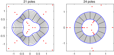
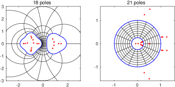
Figure 9: Above, map of a smooth annulus computed by Algorithm P2. Poles of the rational representations of $f$ and $f^{-1}$ appear both inside and outside the annuli. Below, an unbounded smooth doubly-connected geometry mapped via the variant $(\ref{disjoint})$–$(\ref{twoeqs2})$ of Algorithm P2. The point $z=\infty$ is now in the interior of $\Omega$, and its image $f(z)=\exp(a_{0})\approx 0.504$ on the right is a simple pole of $f^{-1}$.

To make (7) and (10) the basis of an algorithm, we set up a least-squares problem whose unknowns are the coefficients $\{a_{k}\}$ and $\{b_{k}\}$ and also the conformal modulus $\rho$. The number of $a_{k}$ and $b_{k}$ coefficients is $N=4n+1$, and the total number of unknowns is $N+1$. The least-squares matrix is of dimensions $2M\times(N+1)$, with the rows corresponding to the $2M$ sample points on the boundary curves and the first $N$ columns containing the values of $\kern 0.7pt\hbox{Re}\kern 0.7pt(z^{k})$ and $\kern 0.7pt\hbox{Im}\kern 0.7pt(z^{k})$ at these points. The final column consists of $M$ zeros and $M$ ones, corresponding to the appearance of $\log\kern 0.7pt\rho$ at one boundary curve but not the other in (7), and the right-hand side is the $2M$-vector consisting of samples on the boundary of $-\log|z|$. Here is the algorithm:

Algorithm P2.

$\bullet$ For $n=$ rounded values of $2^{4},2^{4.5},2^{5},\dots$ until convergence or failure,

- Set $M=8\kern 0.3ptn$ and sample $-\log|z|$ in $M$ points each of $P_{1}$ and $P_{2}$;

- Solve a $2M\times(N+1)$ least-squares problem for the coefficients $a_{k}$ and $b_{k}$ of $(\ref{approxes})$ and the number $\rho$;

$\bullet$ Form $u$ and $v$ from $(\ref{approxes})$ and $f$ from $(\ref{frep})$;

$\bullet$ Approximate $f$ by a AAA rational approximation;

$\bullet$ Approximate $f^{-1}$ by another AAA rational approximation.

Chebfun’s conformal command executes this algorithm when it is called with two boundary arcs rather than one, and the upper half of Figure 9 shows the result computed in about $0.2$ sec. by these Chebfun commands:

    z = chebfun(’exp(1i*pi*z)’,’trig’);
    C1 = z*abs(1+.1*z^4); C2 = .5*z*abs(1+.2*z^3);
    conformal(C1, C2, ’plots’);

So far as I know, Figure 9 is the first illustration ever published of rational approximations with free poles used to represent conformal maps of doubly-connected domains.

There is an alternative doubly-connected geometry which, while mathematically equivalent to the one we have just treated, may in practice be worth considering separately. Suppose that $\Omega$, rather than being the annular region between two concentric curves $P_{1}$ and $P_{2}$, is the infinite region of the extended complex plane exterior to two disjoint curves $P_{1}$ and $P_{2}$. If $P_{1}$ encloses $z=-1$ and $P_{2}$ encloses $z=1$, then we can write the conformal map of $\Omega$ onto a circular annulus in the form

$$f(z)={z-1\over z+1}\kern 1.0pte^{u(z)+iv(z)}$$ (11)

where $u$ is harmonic in $\Omega$ and satisfies, in analogy to (7),

$$u=\cases{-\log\Bigl{|}\displaystyle{z-1\over z+1}\Bigr{|},&$z\in P_{1}$,\cr\vskip 7.0pt\cr-\log\Bigl{|}\displaystyle{z-1\over z+1}\Bigr{|}+\log\kern 0.7pt\rho,&$z\in P_{2}$}$$ (12)

for a value of $\rho$ that again will be uniquely determined. To fashion this into an elementary algorithm based on series, we replace the Laurent polynomials of (10) by polynomials involving negative powers of $z-1$ and $z+1$. The algorithm is otherwise the same, and the second row of Figure 9 shows a computed example. Note that $u$, $v$, and $f$ are regular at $z=\infty$, where they take the values $a_{0}$, $0$, and $\exp(a_{0})$, respectively. Thus the inverse map $f^{-1}$ has a pole in the circular annulus at the point $\exp(a_{0})$, as appears in the plot.

As with its simply connected analogue P1 of Section 2, Algorithm P2 is far from robust, and it will quickly fail if applied to regions much more complicated than those of Figure 9. Superior performance can undoubtedly be achieved with integral equations, though this has not been implemented in Chebfun.

5 Doubly connected domains with corners

By a doubly connected domain with corners, we mean the region $\Omega$ lying between two Jordan curves $P_{1}$ and $P_{2}$ as in the last section, where now, each curve is a finite chain of analytic arcs. To conformally map such a domain, we solve the Dirichlet problem of section 4 by the lightning Laplace solver of section 3, placing poles both outside the corners of $P_{1}$ and inside the corners of $P_{2}$. The algorithm can be summarized as follows.

Algorithm R2.

$\bullet$ Solve $(\ref{twoeqs})$ by the lightning method and form $f$ from (2);

$\bullet$ Approximate $f$ by a AAA rational approximation;

$\bullet$ Approximate $f^{-1}$ by another AAA rational approximation.

The upper part of Figure 10 illustrates such a map for a region that is a polygonal analogue of the region of the first map of Figure 9. As in the last section, there is a straightforward analogue of Algorithm R2 for an unbounded region exterior to two disjoint curves with corners, and this is illustrated in the lower part of Figure 10. Such domains may be of particular interest for the calculation of constants associated with low-rank separability, as discussed by Beckermann, Townsend, and Wilber bt ; tw .

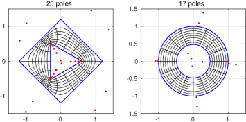
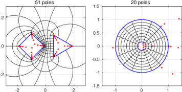
Figure 10: Doubly connected domains with corners mapped by Algorithm R2 and its variant. The function $f^{-1}$ in the lower pair again has a simple pole in the domain, shown by a dot.

For polygonal boundaries as in Figure 10, there is a doubly-connected Schwarz–Christoffel formula dep ; SCbook ; henrici which has been implemented numerically by Däppen daeppen and Hu hu , the latter with a Fortran package DSCPACK.

6 Multiply connected domains

Domains of connectivity higher than two can also be conformally mapped. The Green’s function idea of (7) generalizes to a formula with different constants $\log\rho_{k}$ on each boundary component, as described in henrici and schiffer . Various numerical methods have been developed, and some of them are reviewed in bds . The Schwarz–Christoffel formula has generalizations that have been developed by DeLillo, Crowdy, and others: crowdy and dep2 are just two of many papers in this area. Recently Nasser has released a code PlgCirMap for computing maps of multiply connected domains by means of a fast implementation of an iterative method due to Koebe nasser .

A difficulty with multiply connected conformal mapping is the lack of an entirely natural target domain. In the doubly connected case, the reduction to an annulus gives a useful interpretation in almost any application. For higher connectivity, standard choices of target domains are regions with holes in the form of circular slits (as delivered by the Green’s function), radial slits, or disks. Physical interpretations in such regions are more strained, however, and it is not always clear that much is gained by transplanting a problem such as a partial differential equation from its native multiply-connected geometry to one of these alternatives.

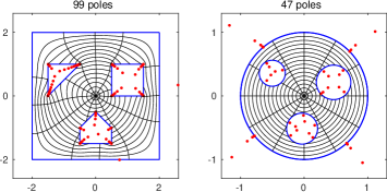
Figure 11: A multiply connected example domain of Nasser nasser . The map is first computed with his PlgCirMap code, and the forward and inverse maps are then approximated by rational functions, with poles as shown. The rational approximations speed up evaluations by a factor of $10$–$20$.

In view of these considerations, we have not extended our numerical methods based on rational functions to multiply-connected regions. If one has computed such a map by an existing method, however, then the possibility remains of compressing it by a subsequent rational approximation as proposed in gt . Figure 11 shows an example. A 4-connected conformal map has been computed by PlgCirMap, and AAA approximation compresses the result to a much more efficient form. Typical times for evaluation of the mapping function or its inverse at each point for this example are on the order of 200 microseconds for PlgCirMap and 10 microseconds for the rational approximations.

7 Numerical details

We now mention some numerical details associated with the algorithms presented in the previous sections. Our implementations are for the most part experimental, however, not claimed to be close to optimal, and we trust that improvements in robustness and accuracy will come in the future.

Accurate data and fine sampling on the boundary. When failure occurs in a lightning Laplace solution, whether for conformal mapping or more generally, the reason is usually that the sampling on the boundary is not fine enough or the sampled data are not accurate enough. In particular, when poles are exponentially clustered near a vertex, it is crucial that the sample points be clustered on the same scale or finer. The laplace software does this automatically according to a scheme described in lightning , and we used the same strategy for the doubly-connected examples of section 5. If the sample points are not dense enough, two things may go wrong: the Laplace problem may be solved inaccurately; and, even if it is accurate, the AAA approximation may fail, with spurious poles appearing in regions where one expects analyticity gt . (By spurious poles we mean poles of very small residue, also known as “Froissart doublets” since they are paired with nearby zeros that nearly cancel their effect.) The latter problem also arises when the grid is fine but the data are insufficiently accurate relative to the scale of the approximation error, so that the AAA algorithm is effectively attempting to approximate a nonanalytic function. Conversely, if the sample points are dense enough and the data accurate enough, spurious poles rarely appear. The mechanism for this is that AAA algorithm delivers a rational approximation with a certain kind of (linearized) optimality. A spurious pole cannot improve an approximation much, so it is unlikely to be present in an optimal approximation. Success cannot be guaranteed, however, as is well known in the theoretical literature on spurious poles in (mostly Padé) rational approximations stahl .

Parameters of AAA approximation. As described in AAA and lawson , Chebfun’s aaa code for AAA approximation has some adjustable parameters. The overall tolerance can be specified, and we have set it equal to the tolerance fixed for the lightning Laplace solver. A “cleanup” option to remove spurious poles is invoked by default, and we have left this in play with its tolerance set equal to the overall AAA tolerance. There is also an option to improve the approximation closer to minimax by a Lawson iteration, and this we have not invoked, because experiments suggest it is ineffective for these problems. All of these choices are experimental, and we have not attempted an analysis that might justify or modify them. As mentioned in the last paragraph, AAA approximation is far from bulletproof. We hope that in the next few years improvements to AAA will be developed, which would have immediate impact on the robustness of our conformal mapping algorithms.

Accuracy and rate of convergence: theory and practice. The theorems of lightning guarantee that Algorithm R1 must converge root-exponentially, i.e. at a rate $C^{\kern 1.0pt-\sqrt{n}}$ for some $C>1$, so long as $\Omega$ is bounded by a finite collection of analytic curves meeting at corners. (We note as before that the statements in lightning assume $\Omega$ is convex, but it is believed that this condition is not actually necessary.) Sometimes, however, convergence stagnates at a low accuracy such as six digits. One reason is that singularities at corners cause ill-conditioning of the conformal map, as does the crowding phenomenon. (A corner of interior angle $\alpha\kern 0.3pt\pi$ with $\alpha<1$ will limit the achievable number of digits to on the order of $\alpha$ times that of machine precision.) Another is that our method relies on the solution of least-squares problems defined by ill-conditioned matrices, though this does not seem to cause much trouble in practice, a phenomenon analyzed in the context of frames in frames .

8 Polygons and circular polygons

In this article we have computed conformal maps by solving Laplace problems via least-squares fitting on the boundary by the “lightning” method of lightning , involving poles exponentially clustered outside $\Omega$. Thus we do not make use of explicit analysis of singularities, as is the more familiar approach in numerical conformal mapping. For polygons, the famous method based on analysis of singularities is the Schwarz–Christoffel formula SCbook , which is realized numerically in the widely used and wonderfully robust SC Toolbox by Driscoll toolbox . For circular polygons, there is an analogous procedure based on the Schwarzian differential equation, though it has had less impact numerically bg ; howell .

For both polygons and circular polygons, an in-between option could be employed that would have some advantages. Locally near a corner $z_{j}$ of a polygon with interior angle $\alpha\kern 0.3pt\pi$ for some $\alpha<2,$ the conformal map will be an analytic function of $(z-z_{j})^{1/\alpha}$ (proof by the Schwarz reflection principle). A similar formula applies at a corner of a circular polygon, derivable by a Möbius transformation to a sector bounded by two straight lines. Thus in both of these cases, one can dispense with exponentially clustered poles outside $\Omega$ and use a series in terms of explicit singularities instead. At the corner of the polygon, for example, the terms will be $(z-z_{j})^{1/\alpha},(z-z_{j})^{2/\alpha},(z-z_{j})^{3/\alpha},\dots.$ By constructing the matrix $A$ from columns corresponding to such terms, one can set up a least-squares problem just as before, but making use of a very different set of basis functions, and the convergence will be exponential rather than root-exponential. This would be a numerical method midway between the traditional Schwarz–Christoffel or Schwarzian differential approaches and the fully general one we have focused on in this paper. (A disadvantage is that the inverse map would have to be treated separately, if AAA rational approximation is to be avoided.) We have not pursued this idea, but proofs of concept for L-shaped and circular L-shaped regions, with short Matlab codes, can be found in example .

One might suppose that these observations indicate that there is no need for lightning Laplace solvers in general when the domain is a polygon or circular polygon. However, this is not so, for the Laplace problems that arise in conformal mapping are special ones, with corner singularities determined only by the local geometry lehman . More general Laplace problems often have different boundary data on different sides of a domain, and in such a case, the corner singularities may be complicated even when the geometry is simple lehman2 .

9 Discussion

The algorithms proposed in this paper combine two phases. First, a Laplace problem is solved by least-squares collocation on the boundary. This is essentially the idea of the Method of Fundamental Solutions, which has been pursued by Amano and his coauthors for conformal mapping amano ; amano2 under the name of the charge simulation method. However, our approach differs in the use of poles exponentially clustered near corner singularities to get root-exponential convergence, as proposed in lightning (or in Section 8, the use of explicit singular terms), and in the use of rational functions (dipoles) rather than point charges (monopoles). Second, the resulting map and its inverse are both approximated by rational functions, as proposed in gt .

The idea of solving Laplace problems by fitting Dirichlet data on the boundary is an old one, and early discussions of note are by Walsh walsh , Curtiss curtiss , Collatz (collatz, , sec. V.4.2), and Gaier (gaier, , sec. 4.1), the last of these specifically for conformal mapping. However, these authors formulated systems of equations rather than least-squares problems, making the method fragile and impractical. As soon as one moves from square matrices and systems of equations to rectangular matrices and least-squares, the distribution of sample points largely ceases to be a problem.

Our methods are based on a minimum of geometrical analysis, and we do not claim they are optimal for any particular problem. For mapping polygons, in particular, the SC Toolbox is tried and true and able to handle quite extreme geometries without difficulty toolbox . Nevertheless, the approach to conformal mapping presented here is very general and usually very fast, enabling typical problems to be solved in on the order of a second of computer time, with subsequent evaluations of both the map and its inverse in microseconds. Experimental codes can be found at lightcode . Extensions to problems such as domains with slits, unbounded domains, or domains bounded by arcs other than straight lines or arcs of circles should be straightforward, though they have not yet been explored.