An Algorithmic View on Optimal Storage Sizing

Abstract

Users can arbitrage against Time-of-Use (ToU) pricing with storage by charging in off-peak period and discharge in peak periods. In this paper we design the optimal control policy and the solve optimal investment for general ToU scheme. We formulate the problem as dynamic programming for efficient solution. Our result is feasible facing multi-peaked ToU scheme. Simulation studies examine how the user’s cost varies with respect to the user’s demand randomness; we also demonstrate the performance of our scheme when aggregating users for extra savings.

I Introduction

High renewable penetration warrants a flexible power system, and storage devices provide most flexibility in the future. The renewables also bring significant uncertainties to power system, which implies dynamic pricing is ideal to reflect the real time market conditions. Hence, storage devices are both desired for future power system as well as future electricity markets.

I-A Opportunities and Challenges

In this paper, we take the first step towards understanding the optimal arbitrage policy with storage system against dynamic pricing. We simplify the problem by eliminating the randomness in dynamic pricing. More precisely, we focus on arbitraging against the general Time-of-Use (ToU) pricing schemes.

Such arbitrage opportunities have been found all over the world (e.g., in US[1], EU[2], and China[3]). However, to design the arbitrage control policy is challenging since the decisions at each period of the ToU scheme are coupled together. When the ToU scheme consists of multiple peaks, the task is even more delicate.

We formulate the problem as dynamic programming (DP) and propose an efficient arbitrage policy for utilizing the storage system. Based on this arbitrage policy, we introduce a binary search algorithm to decide optimal investment storage capacity (storage sizing) in terms of minimizing electricity bills.

I-B Related Work

The major body of literature is on designing the storage control policies under various pricing schemes. Just to name a few, Koutsopoulos et al. propose a control policy for finite capacity storage system for utilities [4]. Van de ven et al. introduce a threshold-based optimal storage control policy facing Markovian prices and demands[5]. Qin et al. design a sub-optimal online greedy algorithm for dynamic pricing and assuming limited information on the demand [6]. Wu et al. solve the optimal storage sizing problem in 3-tier ToU pricing [7]. Different from previous work, we focus on designing the arbitrage policy and solving the optimizing sizing problem in general (multi-peaked) ToU schemes.

Next, we introduce system model in Section II. Section III designs the optimal control policy and derives optimal investment in general ToU pricing. Simulation studies are conducted in Section IV. Section V provides the concluding remarks. Due to space limitations, we provide the sketch of all the proofs in Appendix, and the full proofs in online supplementary material [8].

II System Model

Consider a multi-peaked ToU scheme, where each day is divided into $n$ periods and the electricity rate in $i^{th}$ period is denoted by $\pi_{i}$. We assume each day ends with the off-peak period, i.e., $\pi_{n}=\min_{i}\{\pi_{i}\}$.

Facing such a ToU scheme, a user consumes random demand $X_{i}$ in $i^{th}$ period. Let $f_{i}(\cdot)$ be the probability density function (pdf) of $X_{i}$. Based on the ToU prices and demand distributions, the user may invest a storage with capacity $C$ to reduce its electricity cost. To better utilize the storage, the user need decide how much to charge or discharge at each period. Such decision problems are coupled together through the capacity constraint, i.e., the energy in the storage system cannot be greater than $C$ at all times.

II-A Assumptions

In order to highlight the essence of the problem and simplify our analysis, we make the following assumptions.

A1. The demand is inelastic.

A2. Storage system is lossless, and perfectly efficient in charging and discharging.

A3. The pdf of random demand, $f_{i}(\cdot)$, is continuously differentiable, and we assume $f_{i}(x)>0\Leftrightarrow x\geq 0$.

A4. The demands for different periods are independent.

The first three assumptions are standard in the literature. As for the last one, we will examine the case when the demands are dependent across periods in the simulation.

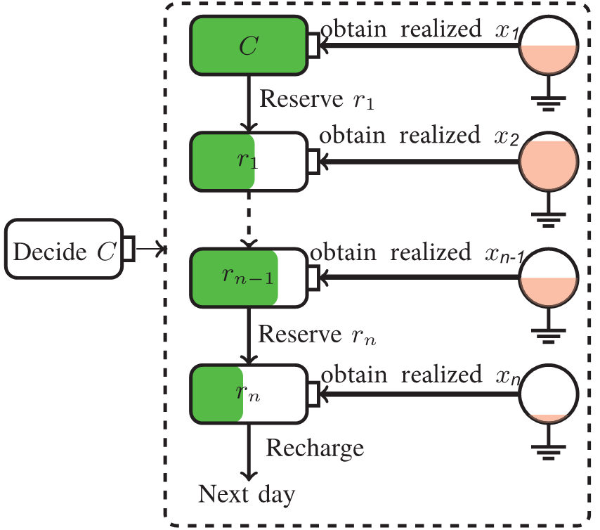
Figure 1: Decision process and DP formulation.

II-B Dynamic Programming Formulation

We consider two sets of decisions: one is the optimal investment for storage, and the other one is the optimal control policy across multiple periods. As for the system model, we focus on understanding the second task, which serves as the basis for solving the first one.

To solve a decision problem across multiple periods, one powerful technique is DP, which simplifies a complicated problem by breaking it down into simpler sub-problems in a recursive manner. In our model, the decision problem is for each user to minimize the expected total cost, while the control space consists of the storage operation strategies at each time slot.

In this paper, we employ a special form of storage operation: reserving energy for future use. That is, at $i^{th}$ period, the user need decide its reservation $r_{i}$ for future use based on the reservation of $(i-1)^{th}$ period (i.e., $r_{i-1}$), and the random demand $X_{i}$. We assume the storage is fully charged at the beginning of each day since each day ends with an off-peak period, and the user will always fully charge the battery during the off-peak. We choose to use $r_{i}^{\prime}s$ to describe the states in DP. It is straightforward to see that the boundary conditions $r_{0}$ and $r_{n}$ are both $C$.

Next, we need identify the cost function for DP: the cost at $i^{th}$ period is due to purchasing $r_{i}+X_{i}-r_{i-1}$ amount of energy from the main grid. Hence, the expected total cost for each user is as follows:

$$J=\mathbb{E}\left[\sum\nolimits_{i=1}^{n}\pi_{i}(r_{i}+X_{i}-r_{i-1})\right].$$ (1)

Due to linearity of expectation and cost function, this problem satisfies the principle of optimality, which yields our DP formulation. We illustrate the process in Fig. 1.

III Optimal Storage Sizing

Based on the DP formulation, we first propose the optimal control policy to utilize the storage system. Then, based on this optimal policy, we solve the optimal storage investment (storage sizing) problem.

III-A Optimal Control Policy

Note that, in our DP formulation, the difficulties are two folded: the decisions are temporally coupled together, and compared with stationary decision making, the decisions can be made in a dynamic fashion as more information is available.

Assuming the user has invested in a storage system with capacity $C$. We focused on stationary control policies (control actions are determined at the beginning of the control horizon and are fixed throughout the horizon), and we use the notion of virtual reservation to decouple the decisions. Later, we will show how to construct the optimal control policy based on the stationary one.

A control policy with virtual reservation $M_{i}$ means that the quantity $M_{i}$ may violate the physical constraints. Hence, at the end of $i^{th}$ period, we project the virtual reservation $M_{i}$ by the capacity constraints, and reserve at least $\min\{M_{i},C\}$ for future use. We first consider a stationary policy, and denote $J_{i}(M_{i}|M_{i+1},\cdots,M_{n})$ as the expected cost after $i^{th}$ period given reservation $M_{i+1},\cdots,M_{n}$. We employ backward induction to decide optimal reservations $M_{i}^{*}$’s. For simplicity, we define

$$J_{i}(M_{i})=J_{i}(M_{i}|M_{i+1}^{*},\cdots,M_{n}^{*}).$$ (2)

With such notations, we can show the following lemmas.

Lemma III.1

If user reserves $M_{i}$ in $i^{th}$ period, then

$$\frac{\mathrm{d}J_{i}}{\mathrm{d}M_{i}}=-\sum\nolimits_{j=i+1}^{n}\pi_{j}P_{j}^{i}(M_{i}),$$ (3)

where $P_{j}^{i}(M_{i})$ denotes the probability that by reserving $M_{i},M^{*}_{i+1},\cdots,M^{*}_{n}$ for future use, $j^{th}$ period is the first period that the user need charge its storage system.

Remark: The economic intuition of this lemma is simply to express the total marginal revenue by reserving additional unit of energy in $i^{th}$ period.

To construct the optimality theorem, we need the following lemma to ensure the uniqueness of our solution.

Lemma III.2

If user reserves $M_{i}\leq C$ in $i^{th}$ period, then

$$\frac{\mathrm{d}^{2}J_{i}}{\mathrm{d}M_{i}^{2}}>0.$$ (4)

With these two lemmas we can prove that a stationary control policy with virtual reservation is optimal. Specifically, if $\pi_{i+1}>\pi_{i}$, the optimal reservation exists and is unique. Otherwise, it is optimal not to reserve, and wait for the next period to directly purchase from the grid. In fact, there exists a sequence of virtual reservation $M^{*}_{i}$ which is optimal for any capacity $C$.

To design an algorithm to obtain this sequence, we first identify the boundary condition: the optimal reservation for the last period must be $C$. Then, we assume that the capacity $C$ is sufficiently large such that all the $M_{i}^{*}$ will be smaller than $C$. In this case, Lemma 4 dictates $M_{i}^{*}$’s, which yields Algorithm 1.

Algorithm 1 Optimal Reservation for $i^{th}$ Period

1:$M^{*}_{i+1},\cdots,M^{*}_{n}$

2:$M^{*}_{i}$

3:if $\pi_{i}\geq\pi_{i+1}$ then

4:     return 0

5:else

6:     solve $M_{i}$ s.t. $\pi_{i}=-\frac{\mathrm{d}J_{i}}{\mathrm{d}M_{i}}$

7:     return $M_{i}$

8:end if

We can solve $M_{i}^{*}$ via binary search since the marginal revenue is monotonic decreasing. To see why Algorithm 1 also works for arbitrary $C$, we make the following observation while deciding $M_{i}^{*}$’s.

Lemma III.3

The optimal reservation $M_{i}^{*}$ by Algorithm 1 depends solely on $M_{j}^{*}$’s where $M_{j}^{*}<M_{i}^{*}$.

That is, for all $M^{*}_{j}\geq M^{*}_{i}$, we do not need their exact values when deciding $M^{*}_{i}$. Hence, combining the physical constraints, we know that all the virtual reservations larger than the capacity $C$ won’t affect the decision process of other virtual reservation. This yields the optimality theorem for Algorithm 1.

Theorem III.4

Algorithm 1 dictates the optimal virtual reservation sequence for any capacity $C$.

III-B Optimal Sizing for Storage Investment

It is straightforward to solve the problem from an economic perspective. The marginal cost to invest additional capacity is the amortized cost of storage system, denoted by $\pi_{s}$. Denote the marginal revenue in $i^{th}$ period by a function in $C$, $MR_{i}(C)$. Classical economic wisdom immediately illustrates a way to decide optimal $C^{*}$:

$$\pi_{s}=\sum\nolimits_{i=1}^{n}MR_{i}(C).$$ (5)

All that remains unknown is to decide $MR_{i}(C)$. In fact, we can use $M_{i}^{*}$’s to help us understand $MR_{i}(C)$. When $M^{*}_{i}\leq C$, more investment won’t lead to any more revenue in $i^{th}$ period. More investment leads to more revenue only at those periods whose virtual reservations are larger than the current capacity $C$. This also illustrates why we stick to use virtual reservation throughout the paper. More specifically,

$$MR_{i}(C)=\begin{cases}0,\ \ \ \ \ \ \ \ \ \ \ \ \ \ \ \ \ \ \ \text{if }M^{*}_{i}\leq C\\ -\frac{\mathrm{d}J_{i}}{\mathrm{d}M_{i}}\big{|}_{M_{i}=C}-\pi_{i},\ \text{otherwise}\end{cases}$$ (6)

Substituting eq. (6) into eq. (5), we can solve the optimal sizing problem via binary search.

Nonetheless, eq. (5) does not always admit a solution due to a too high amortized cost. We seek to give a sufficient and necessary condition to guarantee a solution to eq. (5). This condition is related to the local maximal and local minimal prices.

Corollary III.5

Denote all local maximal prices by $H_{1},\cdots,H_{m}$ and all local minimal prices by $L_{1},\cdots,L_{m}$, then if and only if

$$\pi_{s}\leq\pi_{\max}=\sum\nolimits_{i=1}^{m}(H_{i}-L_{i}),$$ (7)

eq. (5) admits a unique solution.

Remark: Note that $\pi_{\max}$ is the maximal marginal revenue that one unit of storage capacity can achieve. Hence, it is straightforward to see that when the amortized cost $\pi_{s}$ is larger than $\pi_{\max}$, then the user would rather not invest in any storage.

IV Simulation

We evaluate the performance of our proposed scheme with real households’ profile (in summer of 2016) from Austin in Pecan Street [9]. We consider a 4-tier multi-peaked ToU pricing scheme from Ontario Energy Board [10], as shown in Fig. 2. We assume the amortized cost of storage system is 2 ¢/kWh.

Figure 2: Sample multi-peaked ToU pricing scheme.

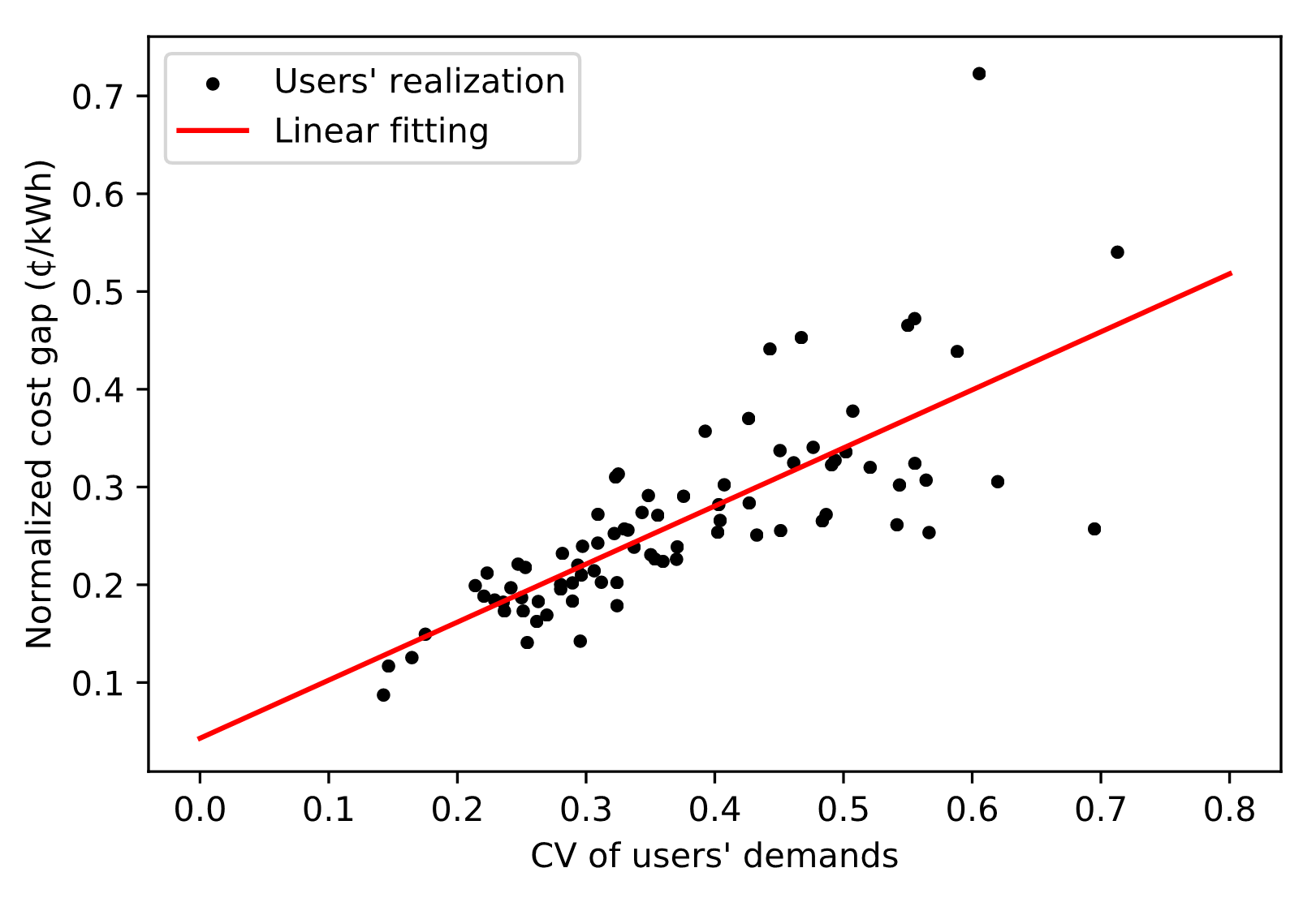
Figure 3: CV v.s. the average cost gap.

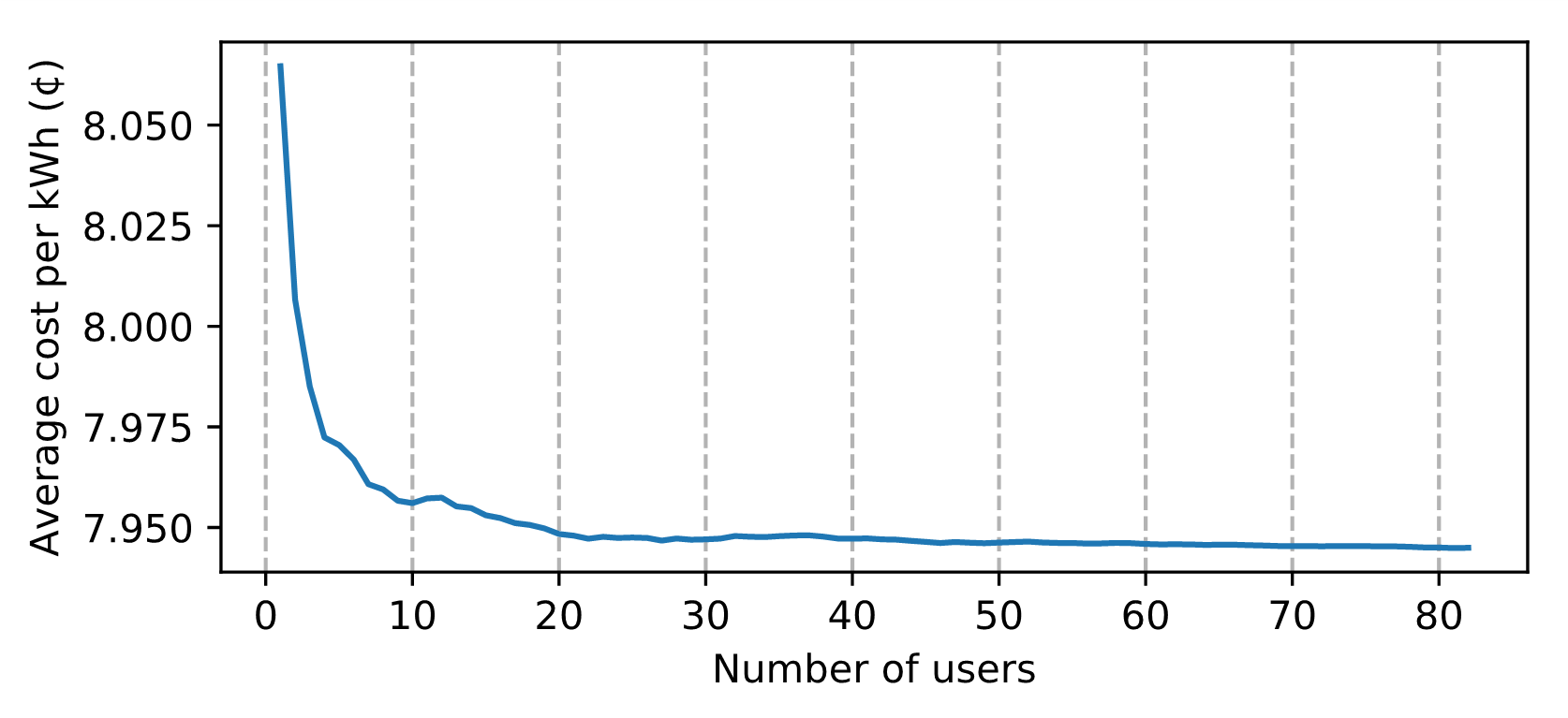
Figure 4: Merge users for more savings.

Figure 3 examines how the user’s cost varies with respect to the user’s demand randomness. We use coefficient of variation (CV) to evaluate such randomness. For each user, we calculate the normalized cost gap between the case of random demands and the case of constant demands (the mean value) to demonstrate the cost savings. It is evident that higher CV leads to higher average cost. That is, for each individual user, it is desirable to reduce its randomness in demand.

However, reducing the randomness may not always be feasible for individual user. One possible way is for individuals to cooperate and merge into a single entity for arbitrage. Figure 4 illustrates that aggregating more users can indeed reduce the average cost. However, such effect is most remarkable till aggregating the first 10 users. This effect diminishes after 20 users’ cooperation. This observation can help decide the effective size of aggregator for arbitrage.

V Conclusion

We investigate the optimal control policy and the optimal storage investment facing general multi-tier ToU pricing. We submit that a sequence of virtual reservations can achieve the most electricity bill savings.

There are quite several interesting future directions. We seek to relax our independent demand assumption and provide more theoretical insights. In this case, a control policy with virtual reservation may not be optimal in that historical information will affect our future reservation.

VI Appendix

VI-A Sketch proof for Lemma III.1

Denote the true reservation by $N_{i}=\min\{M^{*}_{i},C\}$. Then, we know $J_{i}(M_{i})=\sum_{j=i+1}^{n}\pi_{j}\mathbb{E}[u_{j}]$, where $u_{j}$ is the purchase in $j^{th}$ period. More precisely, $\mathbb{E}[u_{j}]$ can be obtained via the law of total probability:

$$\begin{split}J_{i}(M_{i})=\sum_{j=i+1}^{n}\pi_{j}\sum_{\text{all sequence }Q}\mathbb{E}[u_{j}|Q]\cdot\text{Pr}\{Q\},\end{split}$$ (8)

where $Q$ denotes a sequence $i<Q_{1}<\cdots<Q_{m}<j$ and we charge at periods $\{Q_{1},\cdots,Q_{m},j\}$; given $Q$,

$$u_{j}=N_{j}-(N_{Q_{m}}-X_{Q_{m}+1}-\cdots-X_{j-1}).$$

Taking the derivative with respect to $M_{i}$ will lead to our conclusion in Lemma III.1.$\hfill\blacksquare$

VI-B Sketch proof for Lemma 4

From lemma III.1 we have

$$\begin{split}\frac{\mathrm{d}J_{i}}{\mathrm{d}M_{i}}=&-\sum_{j=i+1}^{n}\pi_{j}P_{j}^{i}(M_{i})\end{split}$$ (9)

When computing the second order derivative, the key is to identify that after mathematical manipulation, $\frac{\mathrm{d}^{2}J_{i}}{\mathrm{d}M_{i}^{2}}$ has the following form:

$$\frac{\mathrm{d}^{2}J_{i}}{\mathrm{d}M_{i}^{2}}=\sum\nolimits_{k=i+1}^{n-1}\sum\nolimits_{j=k}^{n}D_{jk},$$ (10)

where

$$\begin{split}\sum_{j=k}^{n}D_{jk}=A_{k}\bigg{(}\pi_{k}-\sum_{j=k+1}^{n}\pi_{j}P_{j}^{k}(N_{k})\bigg{)}\geq 0,\end{split}$$ (11)

and $A_{k}$ is a positive coefficient. The last inequality holds due to the optimality of $N_{k}$. And for period $k=n-1$, this term is strictly positive. Hence, the lemma immediately follows.$\hfill\blacksquare$

VI-C Proof of Lemma III.3

For $j<i$, regardless of exact value of $M^{*}_{j}$, it won’t affect $M^{*}_{i}$. Next, we focus on the case when $j>i$.

When $\pi_{i+1}<\pi_{i}$, it is straightforward to see that we need not reserve anything at $i^{th}$ period, i.e., $M^{*}_{i}=0$. Hence, in this case, regardless of the exact value of $M_{j}^{*}$, it won’t affect $M_{i}^{*}$.

Otherwise, $M^{*}_{i}$ is the unique solution to

$$\pi_{i}=\sum\nolimits_{k=i+1}^{n}\pi_{k}P_{k}^{i}(M_{i}).$$ (12)

And it suffices to show that for $M^{*}_{j}\geq M^{*}_{i}$, all $P_{k}^{i}(M_{i})$’s are irrelevant to $M_{j}^{*}$. By the definition of $P_{k}^{i}(M_{i})$, it is the probability that $k^{th}$ period is the first period that the user need charge the storage. Due to the fact that $M^{*}_{j}\geq M^{*}_{i}$, $P_{k}^{i}(M_{i})=0,\forall k>j$. For $k<j$, $P_{k}^{i}(M_{i})$ is not related to $M^{*}_{j}$. The only remaining hurdle is when $k=j$. Note that

$$\sum\nolimits_{k=i+1}^{n}P_{k}^{i}(M_{i})=1,$$ (13)

we know that

$$P_{j}^{i}(M_{i})=1-\sum\nolimits_{k=i+1}^{j-1}P_{k}^{i}(M_{i}),$$ (14)

which is also irrelevant to $M_{j}^{*}$. Thus, we complete the whole proof.$\hfill\blacksquare$

VI-D Proof of Theorem III.4

We prove the theorem by backward induction. For the last period, the optimal reservation is $C$, which is the boundary of our algorithm, and is optimal.

Suppose the reservation for $i+1^{th}$ period to the last period are all optimal. For $i^{th}$ period, if $M^{*}_{i}>C$, then the marginal revenue must be greater than 0, which implies that reserving $C$ is optimal and the conclusion holds. Otherwise, from Theorem III.3, we know that $M^{*}_{i}$ is not related to the reservation which is greater than $C$. Thus, it suffices to prove the conclusion when the capacity is sufficiently large. Due to induction hypothesis, we can show that reserving $M^{*}_{i}$ is optimal in this case, and also optimal for arbitrary capacity $C$. $\hfill\blacksquare$

VI-E Proof of Corollary III.5

The maximal profit that unit storage can achieve is

$$\sum\nolimits_{i=1}^{n}\max\{\pi_{i+1}-\pi_{i},0\}.$$ (15)

Separating the whole periods by $H_{1},\cdots,H_{m}$ and $L_{1},\cdots,L_{m}$, we can observe that from each local minimal price to local maximal price (rate increasing periods), all the prices between these two periods in (15) can be eliminated. For other periods (rate decreasing periods), $\max\{\pi_{i+1}-\pi_{i},0\}$ is always zero. These two observations immediately lead to our conclusion.$\hfill\blacksquare$

References

- [1] R. Walawalkar, J. Apt, and R. Mancini, “Economics of electric energy storage for energy arbitrage and regulation in new york,” Energy Policy, vol. 35, no. 4, pp. 2558–2568, 2007.
- [2] D. Zafirakis, K. J. Chalvatzis, et al., “The value of arbitrage for energy storage: Evidence from european electricity markets,” Applied energy, vol. 184, pp. 971–986, 2016.
- [3] B. Lin and W. Wu, “Economic viability of battery energy storage and grid strategy: A special case of china electricity market,” Energy, vol. 124, pp. 423–434, 2017.
- [4] I. Koutsopoulos, V. Hatzi, and L. Tassiulas, “Optimal energy storage control policies for the smart power grid,” in Proc. of IEEE SmartGridComm, Oct 2011, pp. 475–480.
- [5] P. M. van de Ven, N. Hegde, L. Massoulié, and T. Salonidis, “Optimal control of end-user energy storage,” IEEE Trans. on Smart Grid, vol. 4, no. 2, pp. 789–797, June 2013.
- [6] J. Qin, Y. Chow, J. Yang, and R. Rajagopal, “Online modified greedy algorithm for storage control under uncertainty,” IEEE Trans. on Power Systems, vol. 31, no. 3, pp. 1729–1743, 2016.
- [7] C. Wu and Y. Yu, “Optimal control for electricity storage against three-tier tou pricing,” in Proc. of APSIPA ASC 2018, pp. 737–741.
- [8] Supplementary material to this article. [Online]. Available: http://iiis.tsinghua.edu.cn/~wu/SM_ISGT_2020.pdf
- [9] Pecan street. [Online]. Available: http://dataport.pecanstreet.org
- [10] Time-of-use price of oeb. [Online]. Available: https://www.oeb.ca/rates-and-your-bill/electricity-rates/historical-electricity-rates