Optimized geometrical metrics satisfying free-stream preservation

Abstract

Computational fluid dynamics and aerodynamics, which complement more expensive empirical approaches, are critical for developing aerospace vehicles. During the past three decades, computational aerodynamics capability has improved remarkably, following advances in computer hardware and algorithm development. However, for complex applications, the demands on computational fluid dynamics continue to increase in a quest to gain a few percent improvements in accuracy. Herein, we numerically demonstrate that optimizing the metric terms which arise from smoothly mapping each cell to a reference element, lead to a solution whose accuracy is practically never worse and often noticeably better than the one obtained using the widely adopted Thomas and Lombard metric terms computation (Geometric conservation law and its application to flow computations on moving grids, AIAA Journal, 1979). Low and high-order accurate entropy stable schemes on distorted, high-order tensor product elements are used to simulate three-dimensional inviscid and viscous compressible test cases for which an analytical solution is known.

1 Introduction

In recent years, with the continuous growth of computing capability and in an effort to achieve more accurate numerical simulations over a broad class of engineering problems, computational fluid dynamics (CFD) has gradually shifted towards high-order accurate simulations; see, for instance, [40, 24, 1]. Modern unstructured high-order methods include discontinuous Galerkin (DG), spectral difference (SD), and flux reconstruction (FR) methods and can produce highly accurate solutions with minimum numerical dispersion and dissipation. Although DG, SD, and FR methods are well suited for smooth solutions, numerical instabilities may occur if the flow contains discontinuities or under-resolved physical features. A variety of mathematical stabilization strategies are commonly used to alleviate these issues (e.g., filtering [22], weighted essentially non-oscillatory schemes [41], artificial dissipation, over-integration, and limiters); however, the use of such techniques for practical complex flow applications often times rely on heuristic (e.g., tunable parameters) or results in schemes that are not always stable (e.g., over-integration)

For the compressible Navier–Stokes equations, a very promising and mathematically rigorous alternative consists in constructing discrete operators that are non-linearly stable (i.e., entropy stable) and simultaneously conserve mass, momentum, and energy, while enforcing a secondary entropy constraint. This strategy consists in first identifying a non-linear neutrally stable flux for the compressible Euler equations, and then adding an appropriate amount of dissipation in order to achieve entropy stability at the semi-discrete level, thus enhancing the stability of the base operator [18, 28, 30, 31]. In this work, we build our study on conforming entropy stable discontinuous collocation methods, constructed by using the summation-by-parts (SBP) operators and the simultaneous-approximation-terms (SAT) framework [5, 28, 7, 26]. However, the proposed methodology can be immediately applied to any of the aforementioned spatial discretization techniques.

In CFD, simulations in complex geometries are performed on the union of piece-wise smooth sub-domains, also called elements or cells, that are smoothly mapped to a reference element. In this element, the derivative terms appearing in the system of partial differential equations (PDEs) are actually evaluated. In the mapped system of equations, the fluxes include the Jacobians of the transformation and the transformation metrics, which depend on derivatives of the transformation. On the one hand, when the element sides are straight, the mapping is linear in each coordinate direction and the metrics are constant. On the other hand, when the element boundaries are curved, these metric terms vary across the element.

At the continuous level, the metric terms naturally satisfy a set of identities [37, 35, 36], and the importance of satisfying these identities at the discrete level has long been recognized; see, for instance, [36, 23, 38]. One of the consequences is that a constant free-stream solution is exactly preserved for all time, independent of the chosen coordinate system. Failure to preserve the free-stream condition frequently leads to spurious source terms that introduce errors in the solution and can be catastrophic in many applications.

The idea of approximating the metric terms in such a way that certain physical quantities are preserved goes back to the early days of CFD. The terminology “geometric conservation law” (GCL) was introduced in 1979 by Thomas and Lombard [35], who found that finite difference approximations that satisfied the metric identities in two dimensions failed in three dimensions. Such observation led to the re-write of the metric terms in a “conservative form”, which, when approximated with central differences, satisfy the metric identities, and thus lead to free-stream preservation. This concept was subsequently extended to geometrically characterize conservative numerical schemes as algorithms that preserve the entire state of a uniform flow.

In previous works [16, 12, 14], the metric terms are constructed for non-conforming discretization at the cell interfaces by solving a strictly convex quadratic optimization problem [9], whose solution guarantees entropy conservation and free-stream preservation. Herein, we numerically show that optimizing the metric terms as proposed in [16, 12, 14] leads, even for conforming interfaces, to a solution whose accuracy is practically never worse and often noticeably better than the one obtained using the widely adopted Thomas and Lombard approach [35]. Thus, we conclude that the pre-processing step of optimizing the metric terms can be used in a computational framework as a unique and viable approach for conforming and $h/p$ non-conforming interfaces. In addition, this choice greatly simplifies the solver and allows important code re-utilization.

The paper is organized as follows. In Section 2 we introduce the notation used in this work. The coordinate transformation from physical to computational space and the key constraints that have to be satisfied by the discrete metric terms are introduced in the context of the linear convection-diffusion equation in Section 3. In the same section, the metric solution mechanics for conforming interior and boundary faces are also presented. Section 4 deals with the compressible Navier–Stokes equations and its semi-discretization using entropy stable SBP-SAT operators of any order. Numerical results for three-dimensional inviscid and viscous test cases for which an analytical solution is known are presented in Section 5. Simulations are performed using low and high-order accurate entropy stable schemes on distorted, high-order tensor product elements [5, 28, 7]. Conclusions are drawn in Section 6.

2 Notation

The notation used in this work has been adopted from [12]. Partial differential equations (PDEs) are discretized on tensor-product cells having Cartesian computational coordinates denoted by the triple $(\xi_{1},\xi_{2},\xi_{3})$, where the physical coordinates are denoted by the triple $(x_{1},x_{2},x_{3})$. Vectors are represented by lowercase bold font, for example $\bm{u}$, while matrices are represented using sans-serif font, for example, $\mathsf{B}$. Continuous functions on a space-time domain are denoted by capital letters in script font. For example,

$$\mathcal{U}\left(\xi_{1},\xi_{2},\xi_{3},t\right)\in L^{2}\left(\left[\alpha_{1},\beta_{1}\right]\times\left[\alpha_{2},\beta_{2}\right]\times\left[\alpha_{3},\beta_{3}\right]\times\left[0,T\right]\right)$$

represents a square integrable function, where $t$ is the temporal coordinate. The restriction of such function onto a set of mesh nodes is denoted by lower case bold font. For example, the restriction of $\mathcal{U}$ onto a grid of $N_{1}\times N_{2}\times N_{3}$ nodes is given by the vector

$$\bm{u}=\left[\mathcal{U}\left(\bm{\xi}^{(1)},t\right),\dots,\mathcal{U}\left(\bm{\xi}^{(N)},t\right)\right]^{\mathrm{T}},$$

where $N$ is the total number of nodes ($N=N_{1}N_{2}N_{3}$), and the square brackets are used to delineate vectors and matrices, as well as ranges for variables (the context will make clear which meaning is being used). Moreover, $\bm{\xi}$ is a vector of vectors constructed from the three vectors $\bm{\xi}_{1}$, $\bm{\xi}_{2}$, and $\bm{\xi}_{3}$, which are vectors of size $N_{1}$, $N_{2}$, and $N_{3}$ and contain the coordinates of the mesh in the three computational directions, respectively. Finally, $\bm{\xi}$ is constructed as

$$\bm{\xi}(3(i-1)+1:3i)=\bm{\xi}^{(i)}=\left[\bm{\xi}_{1}(i),\bm{\xi}_{2}(i),\bm{\xi}_{3}(i)\right]^{\mathrm{T}},$$

where the notation $\bm{u}(i)$ means the $i^{\mathrm{th}}$ entry of the vector $\bm{u}$ and $\bm{u}(i:j)$ is the subvector constructed from $\bm{u}$ using the $i^{\mathrm{th}}$ through $j^{\mathrm{th}}$ entries (i.e., Matlab notation is used).

Oftentimes, monomials are discussed and the following notation is used:

$$\bm{\xi}_{l}^{j}=\left[\left(\bm{\xi}_{l}(1)\right)^{j},\dots,\left(\bm{\xi}_{l}(N_{l})\right)^{j}\right]^{\mathrm{T}},$$

with the convention that $\bm{\xi}_{l}^{j}=\bm{0}$ for $j<0$.

Herein, one-dimensional SBP operators are used to discretize derivatives. The definition of a one-dimensional SBP operator in the $\xi_{l}$ direction, $l=1,2,3$, is [11, 15, 34]

Definition 1.

Summation-by-parts operator for the first derivative: A matrix operator, $\mathsf{D}_{\xi_{l}}^{(1D)}\in\mathbb{R}^{N_{l}\times N_{l}}$, is an SBP operator of degree $p$ approximating the derivative $\frac{\partial}{\partial\xi_{l}}$ on the domain $\xi_{l}\in\left[\alpha_{l},\beta_{l}\right]$ with nodal distribution $\bm{\xi}_{l}$ having $N_{l}$ nodes, if

1. $\mathsf{D}_{\xi_{l}}^{(1D)}\bm{\xi}_{l}^{j}=j\bm{\xi}_{l}^{j-1}$, $j=0,1,\dots,p$;

2. $\mathsf{D}_{\xi_{l}}^{(1D)}=\left(\mathsf{P}_{\xi_{l}}^{(1D)}\right)^{-1}\mathsf{Q}_{\xi_{l}}^{(1D)}$, where the norm matrix, $\mathsf{P}_{\xi_{l}}^{(1D)}$, is symmetric positive definite;

3. $\mathsf{Q}_{\xi_{l}}^{(1D)}=\left(\mathsf{S}_{\xi_{l}}^{(1D)}+\frac{1}{2}\mathsf{E}_{\xi_{l}}^{(1D)}\right)$, $\mathsf{S}_{\xi_{l}}^{(1D)}=-\left(\mathsf{S}_{\xi_{l}}^{(1D)}\right)^{\mathrm{T}}$, $\mathsf{E}_{\xi_{l}}^{(1D)}=\left(\mathsf{E}_{\xi_{l}}^{(1D)}\right)^{\mathrm{T}}$,
   $\mathsf{E}_{\xi_{l}}^{(1D)}=\operatorname{diag}\left(-1,0,\dots,0,1\right)=\bm{e}_{N}\bm{e}_{N}^{\mathrm{T}}-\bm{e}_{1}\bm{e}_{1}^{\mathrm{T}}$, $\bm{e}_{1}=\left[1,0,\dots,0\right]^{\mathrm{T}}$, and $\bm{e}_{N}=\left[0,0,\dots,1\right]^{\mathrm{T}}$.

Thus, a degree $p$ SBP operator is one that differentiates exactly monomials up to degree $p$.

In this work, one-dimensional SBP operators are extended to multiple dimensions using tensor products ($\otimes$). The tensor product between the matrices $\mathsf{A}$ and $\mathsf{B}$ is given as $\mathsf{A}\otimes\mathsf{B}$. When referencing individual entries in a matrix the notation $\mathsf{A}(i,j)$ is used, which means the $i^{\mathrm{th}}$ $j^{\mathrm{th}}$ entry in the matrix $\mathsf{A}$.

The focus of this paper is exclusively on diagonal-norm SBP operators. Moreover, the same one-dimensional SBP operator is used in each direction, each operating on $N_{l}$ nodes. Specifically, diagonal-norm SBP operators constructed on the Legendre–Gauss–Lobatto (LGL) nodes are used, i.e., a discontinuous Galerkin collocated spectral element approach is utilized (see, for instance, [5, 28, 7, 26, 21, 20]).

When solving PDEs numerically, the physical domain $\Omega\subset\mathbb{R}^{3}$, with boundary $\Gamma=\partial\Omega$, with Cartesian coordinates $\left(x_{1},x_{2},x_{3}\right)\subset\mathbb{R}^{3}$, is partitioned into $K$ non-overlapping elements. The domain of the $\kappa^{\text{th}}$ element is denoted by $\Omega_{\kappa}$ and has boundary $\partial\Omega_{\kappa}$. Numerically, we solve PDEs in computational coordinates, $\left(\xi_{1},\xi_{2},\xi_{3}\right)\subset\mathbb{R}^{3}$, where each $\Omega_{\kappa}$ is locally transformed to the reference element $\hat{\Omega}_{\kappa}$, with boundary $\partial\hat{\Omega}_{\kappa}$, using a pull-back curvilinear coordinate transformation which satisfies the following assumption:

Assumption 1.

Each element in physical space is transformed using a local and invertible curvilinear coordinate transformation that is compatible at shared interfaces, meaning that the push-forward element-wise mappings are continuous across physical element interfaces. Note that this is the standard assumption requiring that the curvilinear coordinate transformation is water-tight.

Precisely, one maps from the reference coordinates $\left(\xi_{1},\xi_{2},\xi_{3}\right)\in[-1,1]^{3}$ to the physical element (see Figure 1) by the push-forward transformation

$$\left(x_{1},x_{2},x_{3}\right)=X\left(\xi_{1},\xi_{2},\xi_{3}\right),$$ (1)

which, in the presence of curved elements, is usually a high-order degree polynomial.

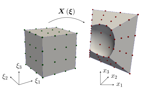
Figure 1: The reference element and its mapping to an element in the mesh.

3 The linear convection-diffusion equation

Many of the technical details for constructing conservative and stable discretizations for the compressible Navier–Stokes, including the metric terms, are present for the discretization of the linear convection-diffusion equation. The linear convection-diffusion equation in Cartesian physical coordinates is given as

$$\frac{\partial\mathcal{U}}{\partial t}+\sum\limits_{m=1}^{3}\frac{\partial\left(a_{m}\mathcal{U}\right)}{\partial x_{m}}=\sum\limits_{m=1}^{3}\frac{\partial^{2}(b_{m}\mathcal{U})}{\partial x_{m}^{2}}, \forall\left(x_{1},x_{2},x_{3}\right)\in\Omega,\quad t\geq 0,$$ (2)

$$\mathcal{U}\left(x_{1},x_{2},x_{3},t\right)={\mathcal{G}}^{(B)}\left(x_{1},x_{2},x_{3},t\right), \forall\left(x_{1},x_{2},x_{3}\right)\in\Gamma,\quad t\geq 0,$$

$$\mathcal{U}\left(x_{1},x_{2},x_{3},0\right)={\mathcal{G}}^{(0)}\left(x_{1},x_{2},x_{3}\right), \forall\left(x_{1},x_{2},x_{3}\right)\in\Omega,$$

where $(a_{m}\mathcal{U})$ are the inviscid fluxes, $a_{m}$ are the (constant) components of the convection speed, $\frac{\partial(b_{m}\mathcal{U})}{\partial x_{m}}$ are the viscous fluxes, and $b_{m}$ are the (constant and positive) diffusion coefficients. The boundary data, ${\mathcal{G}}^{(B)}$, and the initial condition, ${\mathcal{G}}^{(0)}$, are assumed to be in $L^{2}(\Omega)$, with the further assumption that ${\mathcal{G}}^{(B)}$ is prescribed so that either energy conservation or energy stability is achieved.

Since derivatives are approximated with differentiation operators defined in computational space, we use the Jacobian of the push-forward mapping and the chain rule

$$\frac{\partial}{\partial x_{m}}=\sum\limits_{l=1}^{3}\frac{\partial\xi_{l}}{\partial x_{m}}\frac{\partial}{\partial\xi_{l}},\quad\frac{\partial^{2}}{\partial x_{m}^{2}}=\sum\limits_{l,a=1}^{3}\frac{\partial\xi_{l}}{\partial x_{m}}\frac{\partial}{\partial\xi_{l}}\left(\frac{\partial\xi_{a}}{\partial x_{m}}\frac{\partial}{\partial\xi_{a}}\right),$$

to transform Equation (2) from physical to computational space as

$$\mathcal{J}\frac{\partial\mathcal{U}}{\partial t}+\sum\limits_{l,m=1}^{3}\mathcal{J}\frac{\partial\xi_{l}}{\partial x_{m}}\frac{\partial\left(a_{m}\mathcal{U}\right)}{\partial\xi_{l}}=\sum\limits_{l,a,m=1}^{3}\mathcal{J}\frac{\partial\xi_{l}}{\partial x_{m}}\frac{\partial}{\partial\xi_{l}}\left(\frac{\partial\xi_{a}}{\partial x_{m}}\frac{\partial(b_{m}\mathcal{U})}{\partial\xi_{a}}\right),$$ (3)

where $\mathcal{J}$ is the determinant of the metric Jacobian. Bringing the metric terms $\mathcal{J}\frac{\partial\xi_{l}}{\partial x_{m}}$ inside the derivative, and using the product rule, gives

$$\begin{split}\mathcal{J}\frac{\partial\mathcal{U}}{\partial t}+\sum\limits_{l,m=1}^{3}\frac{\partial}{\partial\xi_{l}}\left(\mathcal{J}\frac{\partial\xi_{l}}{\partial x_{m}}a_{m}\mathcal{U}\right)-&\sum\limits_{l,m=1}^{3}a_{m}\mathcal{U}\frac{\partial}{\partial\xi_{l}}\left(\mathcal{J}\frac{\partial\xi_{l}}{\partial x_{m}}\right)=\\ \sum\limits_{l,a,m=1}^{3}\frac{\partial}{\partial\xi_{l}}\left(\mathcal{J}\frac{\partial\xi_{l}}{\partial x_{m}}\frac{\partial\xi_{a}}{\partial x_{m}}\frac{\partial(b_{m}\mathcal{U})}{\partial\xi_{a}}\right)-&\sum\limits_{l,a,m=1}^{3}\frac{\partial\xi_{a}}{\partial x_{m}}\frac{\partial(b_{m}\mathcal{U})}{\partial\xi_{a}}\frac{\partial}{\partial\xi_{l}}\left(\mathcal{J}\frac{\partial\xi_{l}}{\partial x_{m}}\right).\end{split}$$ (4)

The last terms on the left- and right-hand sides of (4) are zero via the GCL relations

$$\sum\limits_{l=1}^{3}\frac{\partial}{\partial\xi_{l}}\left(\mathcal{J}\frac{\partial\xi_{l}}{\partial x_{m}}\right)=0,\quad m=1,2,3,$$ (5)

leading to the strong conservation form of the convection-diffusion equation in computational space

$$\mathcal{J}\frac{\partial\mathcal{U}}{\partial t}+\sum\limits_{l,m=1}^{3}\frac{\partial}{\partial\xi_{l}}\left(\mathcal{J}\frac{\partial\xi_{l}}{\partial x_{m}}a_{m}\mathcal{U}\right)=\sum\limits_{l,a,m=1}^{3}\frac{\partial}{\partial\xi_{l}}\left(\mathcal{J}\frac{\partial\xi_{l}}{\partial x_{m}}\frac{\partial\xi_{a}}{\partial x_{m}}\frac{\partial(b_{m}\mathcal{U})}{\partial\xi_{a}}\right).$$ (6)

Now, consider discretizing Equation (6) by using the following differentiation matrices

$$\mathsf{D}_{\xi_{1}}=\mathsf{D}_{\xi_{1}}^{(1D)}\otimes\mathsf{I}_{N_{2}}\otimes\mathsf{I}_{N_{3}},\;\mathsf{D}_{\xi_{2}}=\mathsf{I}_{N_{1}}\otimes\mathsf{D}_{\xi_{2}}^{(1D)}\otimes\mathsf{I}_{N_{3}},\;\mathsf{D}_{\xi_{3}}=\mathsf{I}_{N_{1}}\otimes\mathsf{I}_{N_{2}}\otimes\mathsf{D}_{\xi_{3}}^{(1D)},$$

where $\mathsf{I}_{N_{l}}$ is an $N_{l}\times N_{l}$ identity matrix and $N_{l}$ is the number of LGL points per direction in a given element. The diagonal matrix containing the metric Jacobian is defined as

$${\color[rgb]{1,.5,0}\mathsf{J}}_{\kappa}=\operatorname{diag}\left(\mathcal{J}(\bm{\xi}^{(1)}),\dots,\mathcal{J}(\bm{\xi}^{(N_{\kappa})})\right),$$

while the diagonal matrix of the metric terms, $\left[{\color[rgb]{0,0,1}\mathcal{J}\frac{\partial\xi_{l}}{\partial x_{m}}}\right]_{\kappa}$, has to be chosen to be a discretization of

$$\operatorname{diag}\left(\mathcal{J}\frac{\partial\xi_{l}}{\partial x_{m}}(\bm{\xi}^{(1)}),\dots,\mathcal{J}\frac{\partial\xi_{l}}{\partial x_{m}}(\bm{\xi}^{(N_{\kappa})})\right),$$

where $N_{\kappa}=N_{1}N_{2}N_{3}$ is the total number of nodes in element $\kappa$. Using this nomenclature, the discretization of (6) on the $\kappa^{\mathrm{th}}$ element reads

$$\begin{split}&{\color[rgb]{1,.5,0}\mathsf{J}}_{\kappa}\frac{\mathrm{d}\bm{u}_{\kappa}}{\mathrm{d}t}+\sum\limits_{l,m=1}^{3}a_{m}\mathsf{D}_{\xi_{l}}\left[{\color[rgb]{0,0,1}\mathcal{J}\frac{\partial\xi_{l}}{\partial x_{m}}}\right]_{\kappa}\bm{u}_{\kappa}=\sum\limits_{l,m,a=1}^{3}b_{m}\mathsf{D}_{\xi_{l}}{\color[rgb]{1,.5,0}\mathsf{J}}_{\kappa}^{-1}\left[{\color[rgb]{0,0,1}\mathcal{J}\frac{\partial\xi_{l}}{\partial x_{m}}}\right]_{\kappa}\left[{\color[rgb]{0,0,1}\mathcal{J}\frac{\partial\xi_{a}}{\partial x_{m}}}\right]_{\kappa}\mathsf{D}_{\xi_{a}}\bm{u}_{\kappa}+\bm{SAT}_{\kappa},\end{split}$$ (7)

where $\bm{SAT}_{\kappa}$ is the vectors of the SATs used to impose boundary conditions and inter-element connectivity [27, 6]. The $\bm{SAT}_{\kappa}$ vector is in general composed from inviscid and viscous contributions, i.e. $\bm{SAT}_{\kappa}=\bm{SAT}^{(I)}_{\kappa}+\bm{SAT}^{(V)}_{\kappa}$.

Unfortunately, the scheme (7) is not guaranteed to be stable. However, a well-known remedy is to canonically split the inviscid terms into one half of the inviscid terms in (3) and one half of the inviscid terms in (4) (see, for instance, [6]), while the viscous terms are treated in strong conservation form. In the continuum, this process leads to

$$\begin{split}&\mathcal{J}\frac{\partial\mathcal{U}}{\partial t}+\frac{1}{2}\sum\limits_{l,m=1}^{3}\left\{\frac{\partial}{\partial\xi_{l}}\left(\mathcal{J}\frac{\partial\xi_{l}}{\partial x_{m}}a_{m}\mathcal{U}\right)+\mathcal{J}\frac{\partial\xi_{l}}{\partial x_{m}}\frac{\partial}{\partial\xi_{l}}\left(a_{m}\mathcal{U}\right)\right\}\\ &-\frac{1}{2}\sum\limits_{l,m=1}^{3}\left\{a_{m}\mathcal{U}\frac{\partial}{\partial\xi_{l}}\left(\mathcal{J}\frac{\partial\xi_{l}}{\partial x_{m}}\right)\right\}=\sum\limits_{l,a,m=1}^{3}\frac{\partial}{\partial\xi_{l}}\left(\mathcal{J}\frac{\partial\xi_{l}}{\partial x_{m}}\frac{\partial\xi_{a}}{\partial x_{m}}\frac{\partial(b_{m}\mathcal{U})}{\partial\xi_{a}}\right),\end{split}$$ (8)

where the last set of terms on the left-hand side are zero by the GCL conditions (5). Then, a stable semi-discrete form is constructed in the same manner as the split form (8) by discretizing the inviscid portion of (3) and (6) using $\mathsf{D}_{\xi_{l}}$, ${\color[rgb]{1,.5,0}\mathsf{J}}_{\kappa}$, and $\left[{\color[rgb]{0,0,1}\mathcal{J}\frac{\partial\xi_{l}}{\partial x_{m}}}\right]_{\kappa}$, and by averaging the results. The viscous terms result from the discretization of the viscous portion of (6). This procedure yields

$$\begin{split}&{\color[rgb]{1,.5,0}\mathsf{J}}_{\kappa}\frac{\mathrm{d}\bm{u}_{\kappa}}{\mathrm{d}t}+\frac{1}{2}\sum\limits_{l,m=1}^{3}a_{m}\left\{\mathsf{D}_{\xi_{l}}\left[{\color[rgb]{0,0,1}\mathcal{J}\frac{\partial\xi_{l}}{\partial x_{m}}}\right]_{\kappa}+\left[{\color[rgb]{0,0,1}\mathcal{J}\frac{\partial\xi_{l}}{\partial x_{m}}}\right]_{\kappa}\mathsf{D}_{\xi_{l}}\right\}\bm{u}_{\kappa}\\ &-\frac{1}{2}\sum\limits_{l,m=1}^{3}\left\{a_{m}\operatorname{diag}\left(\bm{u}_{\kappa}\right)\mathsf{D}_{\xi_{l}}\left[{\color[rgb]{0,0,1}\mathcal{J}\frac{\partial\xi_{l}}{\partial x_{m}}}\right]_{\kappa}\bm{1}_{\kappa}\right\}=\\ &\sum\limits_{l,m,a=1}^{3}b_{m}\mathsf{D}_{\xi_{l}}{\color[rgb]{1,.5,0}\mathsf{J}}_{\kappa}^{-1}\left[{\color[rgb]{0,0,1}\mathcal{J}\frac{\partial\xi_{l}}{\partial x_{m}}}\right]_{\kappa}\left[{\color[rgb]{0,0,1}\mathcal{J}\frac{\partial\xi_{a}}{\partial x_{m}}}\right]_{\kappa}\mathsf{D}_{\xi_{a}}\bm{u}_{\kappa}+\bm{SAT}_{\kappa},\end{split}$$ (9)

where $\bm{1}_{\kappa}$ is a vector of ones of size $N_{\kappa}$.

As in the continuous case, the semi-discrete form has a set of discrete GCL conditions

$$\sum\limits_{l=1}^{3}\mathsf{D}_{\xi_{l}}\left[{\color[rgb]{0,0,1}\mathcal{J}\frac{\partial\xi_{l}}{\partial x_{m}}}\right]_{\kappa}\bm{1}_{\kappa}=\bm{0},\quad m=1,2,3,$$ (10)

that, when satisfied, lead to the following telescoping, provably stable, semi-discrete form

$$\begin{split}&{\color[rgb]{1,.5,0}\mathsf{J}}_{\kappa}\frac{\mathrm{d}\bm{u}_{\kappa}}{\mathrm{d}t}+\frac{1}{2}\sum\limits_{l,m=1}^{3}a_{m}\left\{\mathsf{D}_{\xi_{l}}\left[{\color[rgb]{0,0,1}\mathcal{J}\frac{\partial\xi_{l}}{\partial x_{m}}}\right]_{\kappa}+\left[{\color[rgb]{0,0,1}\mathcal{J}\frac{\partial\xi_{l}}{\partial x_{m}}}\right]_{\kappa}\mathsf{D}_{\xi_{l}}\right\}\bm{u}_{\kappa}=\\ &\sum\limits_{l,m,a=1}^{3}b_{m}\mathsf{D}_{\xi_{l}}{{\color[rgb]{1,.5,0}\mathsf{J}}_{\kappa}}^{-1}\left[{\color[rgb]{0,0,1}\mathcal{J}\frac{\partial\xi_{l}}{\partial x_{m}}}\right]_{\kappa}\left[{\color[rgb]{0,0,1}\mathcal{J}\frac{\partial\xi_{a}}{\partial x_{m}}}\right]_{\kappa}\mathsf{D}_{\xi_{a}}\bm{u}_{\kappa}+\bm{SAT}_{\kappa}.\end{split}$$ (11)

Remark 1.

The linear stability of semi-discrete operators for constant coefficient hyperbolic systems, is not preserved by arbitrary design order approximations of the metric terms. Only approximations to the metric terms that satisfy the discrete GCL conditions (10) lead to stable semi-discrete forms.

Remark 2.

The discrete metrics constructed using the analytic formalism of Vinokur and Yee [39] or Thomas and Lombard [35] will in general satisfy the discrete GCL conditions given by (10) for conforming interfaces when tensor-product differentiation operators are used.

Herein, we optimize the metric terms as presented in [16, 12, 13, 14] using the algorithm of Crean et al. [9]. Only conforming interfaces are considered. In what follows, we show which metric terms are optimized and how this optimization process is performed.

3.1 Review of the inviscid coupling procedure

The key element of the discretization that clearly show the opportunity of optimizing the volume metric terms is the inviscid SAT term. Thus, we consider the discretization of the pure convection equation, i.e., discretization (11) with only the convective contributions:

$$\begin{split}&{\color[rgb]{1,.5,0}\mathsf{J}}_{\kappa}\frac{\mathrm{d}\bm{u}_{\kappa}}{\mathrm{d}t}+\frac{1}{2}\sum\limits_{l,m=1}^{3}a_{m}\left\{\mathsf{D}_{\xi_{l}}\left[{\color[rgb]{0,0,1}\mathcal{J}\frac{\partial\xi_{l}}{\partial x_{m}}}\right]_{\kappa}+\left[{\color[rgb]{0,0,1}\mathcal{J}\frac{\partial\xi_{l}}{\partial x_{m}}}\right]_{\kappa}\mathsf{D}_{\xi_{l}}\right\}\bm{u}_{\kappa}=\bm{SAT}^{(I)}_{\kappa}.\end{split}$$ (12)

Figure 2: Generic vertical interface between two cells in computational space.

Without loss of generality, and for clarity of presentation, we consider only one vertical shared face $f$, as shown in Figure 2. When considering a single set of metrics computed, for instance, with one of the approaches presented in [35] or [39], the inviscid SAT coupling the element $\kappa$ with the neighboring element $\kappa^{\prime}$ is constructed as

$$\begin{split}\bm{SAT}^{(I)}_{\kappa,f}=&+\phantom{\frac{1}{2}}{\mathsf{P}}^{-1}\sum\limits_{m=1}^{3}a_{m}\left\{\left(\bm{e}_{N}\bm{e}_{N}^{\mathrm{T}}\otimes\mathsf{P}_{\xi_{2}}^{(1D)}\otimes\mathsf{P}_{\xi_{3}}^{(1D)}\right)\left[{\color[rgb]{0,0,1}\mathcal{J}\frac{\partial\xi_{l}}{\partial x_{m}}}\right]_{\kappa}\right\}\bm{u}_{\kappa}\\ &-\frac{1}{2}{\mathsf{P}}^{-1}\sum\limits_{m=1}^{3}a_{m}\left\{\left(\bm{e}_{N}\bm{e}_{N}^{\mathrm{T}}\otimes\mathsf{P}_{\xi_{2}}^{(1D)}\otimes\mathsf{P}_{\xi_{3}}^{(1D)}\right)\left[{\color[rgb]{0,0,1}\mathcal{J}\frac{\partial\xi_{l}}{\partial x_{m}}}\right]_{\kappa}\right\}\bm{u}_{\kappa}\\ &-\frac{1}{2}{\mathsf{P}}^{-1}\sum\limits_{m=1}^{3}a_{m}\left\{\left(\bm{e}_{N}\bm{e}_{1}^{\mathrm{T}}\otimes\mathsf{P}_{\xi_{2}}^{(1D)}\otimes\mathsf{P}_{\xi_{3}}^{(1D)}\right)\left[{\color[rgb]{0,0,1}\mathcal{J}\frac{\partial\xi_{l}}{\partial x_{m}}}\right]_{\kappa^{\prime}}\right\}\bm{u}_{\kappa^{\prime}},\end{split}$$ (13)

where $\mathsf{P}=\mathsf{P}_{\xi_{1}}^{(1D)}\otimes\mathsf{P}_{\xi_{2}}^{(1D)}\otimes\mathsf{P}_{\xi_{3}}^{(1D)}$. The action of the operator $\left(\bm{e}_{N}\bm{e}_{N}^{\mathrm{T}}\otimes\mathsf{P}_{\xi_{2}}^{(1D)}\otimes\mathsf{P}_{\xi_{3}}^{(1D)}\right)$ consists in extracting from the volume metrics only the “surface metrics” associated with the LGL points located at the interface of the two cells. Similarly, $\left(\bm{e}_{N}\bm{e}_{1}^{\mathrm{T}}\otimes\mathsf{P}_{\xi_{2}}^{(1D)}\otimes\mathsf{P}_{\xi_{3}}^{(1D)}\right)$ extracts the shared surface metrics terms from the $\kappa^{\prime}$ element. Expression (13) simplifies to the well-known formula [27]

$$\begin{split}\bm{SAT}^{(I)}_{\kappa,f}=&+\frac{1}{2}{\mathsf{P}}^{-1}\sum\limits_{m=1}^{3}a_{m}\left\{\left(\bm{e}_{N}\bm{e}_{N}^{\mathrm{T}}\otimes\mathsf{P}_{\xi_{2}}^{(1D)}\otimes\mathsf{P}_{\xi_{3}}^{(1D)}\right)\left[{\color[rgb]{0,0,1}\mathcal{J}\frac{\partial\xi_{l}}{\partial x_{m}}}\right]_{\kappa}\right\}\bm{u}_{\kappa}\\ &-\frac{1}{2}{\mathsf{P}}^{-1}\sum\limits_{m=1}^{3}a_{m}\left\{\left(\bm{e}_{N}\bm{e}_{1}^{\mathrm{T}}\otimes\mathsf{P}_{\xi_{2}}^{(1D)}\otimes\mathsf{P}_{\xi_{3}}^{(1D)}\right)\left[{\color[rgb]{0,0,1}\mathcal{J}\frac{\partial\xi_{l}}{\partial x_{m}}}\right]_{\kappa^{\prime}}\right\}\bm{u}_{\kappa^{\prime}}.\end{split}$$ (14)

In this work, the convective term $\bm{SAT}^{(I)}_{\kappa,f}$ is instead constructed by using two different set of metrics

$$\begin{split}\bm{SAT}^{(I)}_{\kappa,f}=&+\phantom{\frac{1}{2}}{\mathsf{P}}^{-1}\sum\limits_{m=1}^{3}a_{m}\left\{\left(\bm{e}_{N}\bm{e}_{N}^{\mathrm{T}}\otimes\mathsf{P}_{\xi_{2}}^{(1D)}\otimes\mathsf{P}_{\xi_{3}}^{(1D)}\right)\left[{\color[rgb]{0,0,1}\mathcal{J}\frac{\partial\xi_{l}}{\partial x_{m}}}\right]_{\kappa}\right\}\bm{u}_{\kappa}\\ &-\frac{1}{2}{\mathsf{P}}^{-1}\sum\limits_{m=1}^{3}a_{m}\left\{\left(\bm{e}_{N}\bm{e}_{N}^{\mathrm{T}}\otimes\mathsf{P}_{\xi_{2}}^{(1D)}\otimes\mathsf{P}_{\xi_{3}}^{(1D)}\right)\left[{\color[rgb]{1,0,0}\mathcal{J}\frac{\partial\xi_{l}}{\partial x_{m}}}\right]_{\kappa}\right\}\bm{u}_{\kappa}\\ &-\frac{1}{2}{\mathsf{P}}^{-1}\sum\limits_{m=1}^{3}a_{m}\left\{\left(\bm{e}_{N}\bm{e}_{1}^{\mathrm{T}}\otimes\mathsf{P}_{\xi_{2}}^{(1D)}\otimes\mathsf{P}_{\xi_{3}}^{(1D)}\right)\left[{\color[rgb]{1,0,0}\mathcal{J}\frac{\partial\xi_{l}}{\partial x_{m}}}\right]_{\kappa^{\prime}}\right\}\bm{u}_{\kappa^{\prime}},\end{split}$$ (15)

where the red metric terms are the analytic metrics, i.e., the metrics computed by differentiating the inverse of the mapping (1). Thus, the discretization of the $\kappa$ element with the inviscid SAT contribution coming only from the shared vertical interface reads

$$\begin{split}{\color[rgb]{1,.5,0}\mathsf{J}}_{\kappa}\frac{\mathrm{d}\bm{u}_{\kappa}}{\mathrm{d}t}&+\frac{1}{2}\sum\limits_{l,m=1}^{3}a_{m}\left\{\mathsf{D}_{\xi_{l}}\left[{\color[rgb]{0,0,1}\mathcal{J}\frac{\partial\xi_{l}}{\partial x_{m}}}\right]_{\kappa}+\left[{\color[rgb]{0,0,1}\mathcal{J}\frac{\partial\xi_{l}}{\partial x_{m}}}\right]_{\kappa}\mathsf{D}_{\xi_{l}}\right\}\bm{u}_{\kappa}=\\ &+\phantom{\frac{1}{2}}{\mathsf{P}}^{-1}\sum\limits_{m=1}^{3}a_{m}\left\{\left(\bm{e}_{N}\bm{e}_{N}^{\mathrm{T}}\otimes\mathsf{P}_{\xi_{2}}^{(1D)}\otimes\mathsf{P}_{\xi_{3}}^{(1D)}\right)\left[{\color[rgb]{0,0,1}\mathcal{J}\frac{\partial\xi_{l}}{\partial x_{m}}}\right]_{\kappa}\right\}\bm{u}_{\kappa}\\ &-\frac{1}{2}{\mathsf{P}}^{-1}\sum\limits_{m=1}^{3}a_{m}\left\{\left(\bm{e}_{N}\bm{e}_{N}^{\mathrm{T}}\otimes\mathsf{P}_{\xi_{2}}^{(1D)}\otimes\mathsf{P}_{\xi_{3}}^{(1D)}\right)\left[{\color[rgb]{1,0,0}\mathcal{J}\frac{\partial\xi_{l}}{\partial x_{m}}}\right]_{\kappa}\right\}\bm{u}_{\kappa}\\ &-\frac{1}{2}{\mathsf{P}}^{-1}\sum\limits_{m=1}^{3}a_{m}\left\{\left(\bm{e}_{N}\bm{e}_{1}^{\mathrm{T}}\otimes\mathsf{P}_{\xi_{2}}^{(1D)}\otimes\mathsf{P}_{\xi_{3}}^{(1D)}\right)\left[{\color[rgb]{1,0,0}\mathcal{J}\frac{\partial\xi_{l}}{\partial x_{m}}}\right]_{\kappa^{\prime}}\right\}\bm{u}_{\kappa^{\prime}}.\end{split}$$ (16)

Further details on how to compute the blue metric terms will be presented in the Section 3.3.

3.2 Review of the coupling procedure for the convection-diffusion equation

In contrast to the metrics for the inviscid terms, the metrics used for the viscous terms need only be, at worst, consistent and design order approximations. Herein, we use the analytic metrics for the viscous terms calculation. To make the presentation easier and to introduce the discretization that will later be used for the viscous portion of the compressible Navier–Stokes equations, the inviscid term is lumped into $\mathcal{I}^{(I)}$ while the viscous terms are simplified. Thus, Equation (8) reduces to

$$\begin{split}&\mathcal{J}\frac{\partial\mathcal{U}}{\partial t}+\mathcal{I}^{(I)}=\sum\limits_{l,a=1}^{3}\frac{\partial}{\partial\xi_{l}}\left(\hat{\mathcal{C}}_{l,a}\Theta_{a}\right),\\ &\hat{\mathcal{C}}_{l,a}=\sum\limits_{m=1}^{3}\mathcal{J}\frac{\partial\xi_{l}}{\partial x_{m}}\frac{\partial\xi_{a}}{\partial x_{m}}b_{m},\quad\Theta_{a}=\frac{\partial\mathcal{U}}{\partial\xi_{a}}.\end{split}$$ (17)

A local discontinuous Galerkin (LDG) and interior penalty approach (IP) approach are used (see references [27, 6, 26]). In the LDG approach, the discretization of the viscous terms in Equation (17) proceeds in two steps. First, the gradients $\Theta_{a}$ are discretized, then the derivatives of the viscous fluxes are discretized. Notice that all the metric terms are contained in $\hat{\mathcal{C}}_{l,a}$, and therefore the critical requirement for stability is to use an SBP operator [27, 6, 16]. Plugging everything together, the final discretization reads

$${\color[rgb]{1,.5,0}\mathsf{J}}_{\kappa}\frac{\mathrm{d}\bm{u}_{\kappa}}{\mathrm{d}t}+\bm{I}^{(I)}_{\kappa}=\sum\limits_{l,a=1}^{3}\mathsf{D}_{\xi_{l}}\left[{\color[rgb]{1,0,0}\hat{\mathcal{C}}_{l,a}}\right]_{\kappa}\bm{\theta}_{a}^{\kappa}\>+\>\bm{SAT}^{(I)}_{\kappa}+\bm{SAT}^{(V)}_{\kappa},\quad\bm{\theta}_{a}^{\kappa}=\mathsf{D}_{\xi_{a}}\bm{u}_{\kappa}+\bm{SAT}^{\theta}_{\kappa},$$ (18)

where the inviscid contributions are contained in $\bm{I}^{(I)}_{\kappa}$, while $\bm{SAT}^{\theta}_{\kappa}$ contains the LDG penalty on the gradient of the entropy variables [27]. The viscous coefficient matrices $\left[{\color[rgb]{1,0,0}\hat{\mathcal{C}}_{l,a}}\right]_{\kappa}$ have been highlighted in red to emphasize that they are computed using the analytic metrics. However, any other design order choice would suffice. The proposed discretization of the viscous terms telescopes the viscous fluxes to the boundary and adds a dissipative term [27]. Thus, it mimics the continuous energy analysis, and leads to a provably energy stable discretization, provided appropriate boundary SATs are used.

3.3 Metric solution mechanics

Here we demonstrate the proposed approach for the approximation of the metric terms, and we consider the discrete GCL conditions (10) associated with Equation (16). By construction, the analytic metric terms are continuous at the interface of the two elements because the curvilinear coordinate transformation (1) is water-tight (see Assumption 1). Thus the GCL constraints read

$$\begin{split}\mathsf{P}\sum\limits_{l=1}^{3}\mathsf{D}_{\xi_{l}}\left[{\color[rgb]{0,0,1}\mathcal{J}\frac{\partial\xi_{l}}{\partial x_{m}}}\right]_{\kappa}\bm{1}_{\kappa}=&+\left\{\left(\bm{e}_{N}\bm{e}_{N}^{\mathrm{T}}\otimes\mathsf{P}_{\xi_{2}}^{(1D)}\otimes\mathsf{P}_{\xi_{3}}^{(1D)}\right)\left[{\color[rgb]{0,0,1}\mathcal{J}\frac{\partial\xi_{l}}{\partial x_{m}}}\right]_{\kappa}\right\}\bm{1}_{\kappa}\\ &-\left\{\left(\bm{e}_{N}\bm{e}_{1}^{\mathrm{T}}\otimes\mathsf{P}_{\xi_{2}}^{(1D)}\otimes\mathsf{P}_{\xi_{3}}^{(1D)}\right)\left[{\color[rgb]{1,0,0}\mathcal{J}\frac{\partial\xi_{l}}{\partial x_{m}}}\right]_{\kappa^{\prime}}\right\}\bm{1}_{\kappa},\\ &m=1,2,3.\end{split}$$ (19)

Equation (19) can be algebraically manipulated into a form that is more convenient for constructing a solution procedure for the metric terms. Multiplying Equation (19) by $-1$, using the SBP property $\mathsf{Q}_{\xi_{l}}^{(1D)}=-{\mathsf{Q}_{\xi_{l}}^{(1D)}}^{\mathrm{T}}+\mathsf{E}_{\xi_{l}}^{(1D)}$, and by canceling common terms, we arrive at

$$\begin{split}\sum\limits_{l=1}^{3}\mathsf{Q}_{\xi_{l}}^{\mathrm{T}}\left[{\color[rgb]{0,0,1}\mathcal{J}\frac{\partial\xi_{l}}{\partial x_{m}}}\right]_{\kappa}\bm{1}_{\kappa}=\left\{\left(\bm{e}_{N}\bm{e}_{1}^{\mathrm{T}}\otimes\mathsf{P}_{\xi_{2}}^{(1D)}\otimes\mathsf{P}_{\xi_{3}}^{(1D)}\right)\left[{\color[rgb]{1,0,0}\mathcal{J}\frac{\partial\xi_{l}}{\partial x_{m}}}\right]_{\kappa^{\prime}}\right\}\bm{1}_{\kappa},\quad m=1,2,3,\end{split}$$ (20)

where $\mathsf{Q}_{\xi_{1}}=\mathsf{Q}_{\xi_{1}}^{(1D)}\otimes\mathsf{P}_{\xi_{2}}^{(1D)}\otimes\mathsf{P}_{\xi_{3}}^{(1D)}$, $\mathsf{Q}_{\xi_{2}}=\mathsf{P}_{\xi_{1}}^{(1D)}\otimes\mathsf{Q}_{\xi_{2}}^{(1D)}\otimes\mathsf{P}_{\xi_{3}}^{(1D)}$, $\mathsf{Q}_{\xi_{3}}=\mathsf{P}_{\xi_{1}}^{(1D)}\otimes\mathsf{P}_{\xi_{2}}^{(1D)}\otimes\mathsf{Q}_{\xi_{3}}^{(1D)}$.

A close examination of (20) shows that the GCL constraints form a highly under-determined system for the unknown metric terms on the left-hand side. Our strategy consists of solving a strictly convex quadratic optimization problem that minimizes the difference between the numerical and analytic volume metrics [9]:

$$\begin{split}&\min_{\bm{a}_{m}}\frac{1}{2}\left(\bm{a}_{m}-\bm{a}_{m,\text{target}}\right)^{\mathrm{T}}\left(\bm{a}_{m}-\bm{a}_{m,\text{target}}\right),\quad\text{subject to}\quad\mathsf{M}\bm{a}_{m}=\bm{c}_{m},\\ &m=1,2,3,\end{split}$$ (21)

where $\bm{a}_{m}$ is a vector of size $3N_{\kappa}$ containing the optimized metrics, i.e.,

$$\left(\bm{a}_{m}\right)^{\mathrm{T}}=\bm{1}^{\mathrm{T}}\left[\left[{\color[rgb]{0,0,1}\mathcal{J}\frac{\partial\xi_{1}}{\partial x_{m}}}\right]_{\kappa},\left[{\color[rgb]{0,0,1}\mathcal{J}\frac{\partial\xi_{2}}{\partial x_{m}}}\right]_{\kappa},\left[{\color[rgb]{0,0,1}\mathcal{J}\frac{\partial\xi_{3}}{\partial x_{m}}}\right]_{\kappa}\right]$$

and $\bm{a}_{m,\text{target}}$ are the targeted, analytical metrics, i.e.

$$\left(\bm{a}_{m,\text{target}}\right)^{\mathrm{T}}=\bm{1}^{\mathrm{T}}\left[\left[{\color[rgb]{1,0,0}\mathcal{J}\frac{\partial\xi_{1}}{\partial x_{m}}}\right]_{\kappa},\left[{\color[rgb]{1,0,0}\mathcal{J}\frac{\partial\xi_{2}}{\partial x_{m}}}\right]_{\kappa},\left[{\color[rgb]{1,0,0}\mathcal{J}\frac{\partial\xi_{3}}{\partial x_{m}}}\right]_{\kappa}\right].$$

The constraints $\mathsf{M}\bm{a}_{m}=\bm{c}_{m}$ are simply the discrete GCL conditions (20). Specifically, the matrix $\mathsf{M}$ is of size $N_{\kappa}\times 3N_{\kappa}$, and it is defined as

$$\mathsf{M}=\left[\mathsf{Q}_{\xi_{1}}^{\mathrm{T}},\mathsf{Q}_{\xi_{2}}^{\mathrm{T}},\mathsf{Q}_{\xi_{3}}^{\mathrm{T}}\right],$$ (22)

while the right-hand side data for the constrained equations, $\bm{c}_{m}$, is a vector of size $N_{\kappa}$ defined as

$$\bm{c}_{m}=\frac{1}{2}\left\{\left(\bm{e}_{N}\bm{e}_{1}^{\mathrm{T}}\otimes\mathsf{P}_{\xi_{2}}^{(1D)}\otimes\mathsf{P}_{\xi_{3}}^{(1D)}\right)\left[{\color[rgb]{1,0,0}\mathcal{J}\frac{\partial\xi_{l}}{\partial x_{m}}}\right]_{\kappa^{\prime}}\right\}\bm{1}_{\kappa}.$$ (23)

The optimal solution of the constrained minimization problem is given by (see Proposition $1$ in [9])

$$\bm{a}_{m}=\bm{a}_{m,\text{target}}-{\mathsf{M}}^{\dagger}\left(\mathsf{M}\bm{a}_{m,\text{target}}-\bm{c}_{m}\right),$$ (24)

with ${\mathsf{M}}^{\dagger}$ the Moore-Penrose pseudo-inverse of $\mathsf{M}$.

4 Discretization of the compressible Navier–Stokes equations

In this section, the algorithm for the convection-diffusion equation presented in the previous section is applied to the compressible Navier–Stokes equations with conforming interfaces. These equations in Cartesian coordinates read

$$\frac{\partial\bm{\mathcal{Q}}}{\partial t}+\sum\limits_{m=1}^{3}\frac{\partial\bm{\mathcal{F}}_{x_{m}}^{(I)}}{\partial x_{m}}=\sum\limits_{m=1}^{3}\frac{\partial\bm{\mathcal{F}}_{x_{m}}^{(V)}}{\partial x_{m}}, \forall\left(x_{1},x_{2},x_{3}\right)\in\Omega,\quad t\geq 0,$$ (25)

$$\bm{\mathcal{Q}}\left(x_{1},x_{2},x_{3},t\right)=\bm{\mathcal{G}}^{(B)}\left(x_{1},x_{2},x_{3},t\right), \forall\left(x_{1},x_{2},x_{3}\right)\in\Gamma,\quad t\geq 0,$$

$$\bm{\mathcal{Q}}\left(x_{1},x_{2},x_{3},0\right)=\bm{\mathcal{G}}^{(0)}\left(x_{1},x_{2},x_{3}\right), \forall\left(x_{1},x_{2},x_{3}\right)\in\Omega,$$

where the vectors $\bm{\mathcal{Q}}$, $\bm{\mathcal{F}}_{x_{m}}^{(I)}$ and $\bm{\mathcal{F}}_{x_{m}}^{(V)}$ denote the conserved variables, the inviscid fluxes, and the viscous fluxes, respectively. The boundary data, $\bm{\mathcal{G}}^{(B)}$, and the initial condition, $\bm{\mathcal{G}}^{(0)}$, are assumed to be in $L^{2}(\Omega)$, with the further assumption that $\bm{\mathcal{G}}^{(B)}$ will be set to coincide with linear, well-posed boundary conditions, prescribed in such a way that either entropy conservation or entropy stability is achieved.

The vector of conserved variables is given by

$$\bm{\mathcal{Q}}=\left[\rho,\rho\mathcal{U}_{1},\rho\mathcal{U}_{2},\rho\mathcal{U}_{3},\rho\mathcal{E}\right]^{\mathrm{T}},$$

where $\rho$ denotes the density, $\bm{\mathcal{U}}=\left[\mathcal{U}_{1},\mathcal{U}_{2},\mathcal{U}_{3}\right]^{\mathrm{T}}$ is the velocity vector, and $\mathcal{E}$ is the specific total energy. The inviscid fluxes are given as

$$\begin{split}\bm{\mathcal{F}}_{x_{m}}^{(I)}=&\left[\rho\mathcal{U}_{m},\rho\mathcal{U}_{m}\mathcal{U}_{1}+\delta_{m,1}\mathcal{P},\rho\mathcal{U}_{m}\mathcal{U}_{2}+\delta_{m,2}\mathcal{P},\right.\left.\rho\mathcal{U}_{m}\mathcal{U}_{3}+\delta_{m,3}\mathcal{P},\rho\mathcal{U}_{m}\mathcal{H}\right]^{\mathrm{T}},\end{split}$$

where $\mathcal{P}$ is the pressure, $\mathcal{H}$ is the specific total enthalpy and $\delta_{i,j}$ is the Kronecker delta.

The required constituent relations are

$$\mathcal{H}=c_{\mathcal{P}}\mathcal{T}+\frac{1}{2}\bm{\mathcal{U}}^{\mathrm{T}}\bm{\mathcal{U}},\quad\mathcal{P}=\rho R\mathcal{T},\quad R=\frac{R_{u}}{M_{w}},$$

where $\mathcal{T}$ is the temperature, $R_{u}$ is the universal gas constant, $M_{w}$ is the molecular weight of the gas, and $c_{\mathcal{P}}$ is the specific heat capacity at constant pressure. Finally, the specific thermodynamic entropy is given as

$$s=\frac{R}{\gamma-1}\log\left(\frac{\mathcal{T}}{\mathcal{T}_{\infty}}\right)-R\log\left(\frac{\rho}{\rho_{\infty}}\right),\quad\gamma=\frac{c_{p}}{c_{p}-R},$$

where $\mathcal{T}_{\infty}$ and $\rho_{\infty}$ are the reference temperature and density, respectively (the stipulated convention has been broken here and $s$ has been used rather than $\mathcal{S}$ for reasons that will be clear next).

The viscous fluxes $\bm{\mathcal{F}}_{x_{m}}^{(V)}$ are given by

$$\bm{\mathcal{F}}_{x_{m}}^{(V)}=\left[0,\tau_{1,m},\tau_{2,m},\tau_{3,m},\sum\limits_{i=1}^{3}\tau_{i,m}\mathcal{U}_{i}-\kappa\frac{\partial\mathcal{T}}{\partial x_{m}}\right]^{\mathrm{T}},$$ (26)

while the viscous stresses are defined as

$$\tau_{i,j}=\mu\left(\frac{\partial\mathcal{U}_{i}}{\partial x_{j}}+\frac{\partial\mathcal{U}_{j}}{\partial x_{i}}-\delta_{i,j}\frac{2}{3}\sum\limits_{n=1}^{3}\frac{\partial\mathcal{U}_{n}}{\partial x_{n}}\right),$$ (27)

where $\mu(\mathcal{T})$ is the dynamic viscosity and $\kappa(\mathcal{T})$ is the thermal conductivity.

The compressible Navier–Stokes equations given in (29) have a convex extension, that when integrated over the physical domain, $\Omega$, depends only on the boundary data and negative semi-definite dissipation terms. This convex extension depends on an entropy function, $\mathcal{S}$, that is constructed from the thermodynamic entropy as

$$\mathcal{S}=-\rho s,$$

and provides a mechanism for proving stability in the $L^{2}$ norm. The entropy variables $\bm{\mathcal{W}}$ are an alternative variable set related to the conservative variables via a one-to-one mapping. They are defined in terms of the entropy function $\mathcal{S}$ by the relation $\bm{\mathcal{W}}^{\mathrm{T}}=\partial\mathcal{S}/\partial\bm{\mathcal{Q}}$ and they are extensively used in the entropy stability proofs of the algorithms used herein; see for instance [5, 26, 19, 14]. In addition, they simultaneously symmetrize the inviscid and the viscous flux Jacobians in all three spatial directions. Further details on continuous entropy analysis are available elsewhere [10, 28, 6].

The entropy stability for the viscous terms in the compressible Navier–Stokes equations (29) is readily demonstrated by exploiting the symmetrizing properties of the entropy variables. Thus, we recast the viscous fluxes in terms of the entropy variables

$$\bm{\mathcal{F}}_{x_{=}}^{(V)}\sum\limits_{j=1}^{3}\mathsf{C}_{m,j}\frac{\partial\bm{\mathcal{W}}}{\partial x_{j}},$$ (28)

with the flux Jacobian matrices satisfying $\mathsf{C}_{m,j}\>=\>{(\mathsf{C}_{j,m})}^{\mathrm{T}}$.

Furthermore, in order to apply the algorithm outlined for the convection-diffusion case (18) to the compressible Navier–Stokes equations, we have to recast system (25) in a skew-symmetric form with respect to the metric terms. This procedure results in

$$\begin{split}&\mathcal{J}\frac{\partial\bm{\mathcal{Q}}}{\partial t}+\sum\limits_{l,m=1}^{3}\frac{1}{2}\frac{\partial}{\partial\xi_{l}}\left(\mathcal{J}\frac{\partial\xi_{l}}{\partial x_{m}}\bm{\mathcal{F}}_{x_{m}}^{(I)}\right)+\frac{1}{2}\mathcal{J}\frac{\partial\xi_{l}}{\partial x_{m}}\frac{\partial\bm{\mathcal{F}}_{x_{m}}^{(I)}}{\partial\xi_{l}}=\sum\limits_{l,m=1}^{3}\frac{\partial}{\partial\xi_{l}}\left(\mathcal{J}\frac{\partial\xi_{l}}{\partial x_{m}}\bm{\mathcal{F}}_{x_{m}}^{(V)}\right)\end{split},$$ (29)

where the GCL relations given in (5) are used to obtain (30) from the divergence form (25). Substituting (28) into (29), we arrive at the system of equations

$$\begin{split}&\mathcal{J}\frac{\partial\bm{\mathcal{Q}}}{\partial t}+\sum\limits_{l,m=1}^{3}\frac{1}{2}\frac{\partial}{\partial\xi_{l}}\left(\mathcal{J}\frac{\partial\xi_{l}}{\partial x_{m}}\bm{\mathcal{F}}_{x_{l}}\right)+\frac{1}{2}\mathcal{J}\frac{\partial\xi_{l}}{\partial x_{m}}\frac{\partial\bm{\mathcal{F}}_{x_{m}}}{\partial\xi_{l}}=\sum\limits_{l,a=1}^{3}\frac{\partial}{\partial\xi_{l}}\left(\hat{\mathsf{C}}_{l,a}\frac{\partial\bm{\mathcal{W}}}{\partial\xi_{a}}\right),\end{split}$$ (30)

where

$$\hat{\mathsf{C}}_{l,a}=\mathcal{J}\frac{\partial\xi_{l}}{\partial x_{m}}\sum\limits_{m,j=1}^{3}\mathsf{C}_{m,j}\frac{\partial\xi_{a}}{\partial x_{j}}.$$ (31)

The symmetric properties of the viscous flux Jacobians are preserved by the rotation into curvilinear coordinates, i.e. $\hat{\mathsf{C}}_{l,a}\>=\>{(\hat{\mathsf{C}}_{a,l})}^{\mathrm{T}}$. We remark that this form of the equations, i.e. skew-symmetric form plus the quadratic form of the viscous terms, is necessary for the construction of the entropy stable schemes used in this work. For further details on the derivation of these viscous coefficient matrices see [17, 28].

Without loss of generality, as was done for the linear convection-diffusion equation, we consider only the coupling SAT terms for one shared interface. Thus, the discretization of the compressible Euler equations, i.e., the inviscid part of (30), is given by

$$\begin{split}&{\color[rgb]{1,.5,0}\mathsf{J}}_{\kappa}\frac{\mathrm{d}\bm{q}_{\kappa}}{\mathrm{d}t}+\frac{1}{2}\sum\limits_{l,m=1}^{3}\left(\mathsf{D}_{\xi_{l}}\left[{\color[rgb]{0,0,1}\mathcal{J}\frac{\partial\xi_{l}}{\partial x_{m}}}\right]_{\kappa}+\left[{\color[rgb]{0,0,1}\mathcal{J}\frac{\partial\xi_{m}}{\partial x_{l}}}\right]_{\kappa}\mathsf{D}_{\xi_{l}}\right)\circ\mathsf{F}_{x_{m}}\left(\bm{q}_{\kappa},\bm{q}_{\kappa}\right)\bm{1}_{\kappa}=\\ &+\phantom{\frac{1}{2}}\mathsf{P}^{-1}\sum\limits_{m=1}^{3}\left\{\left(\bm{e}_{N}\bm{e}_{N}^{\mathrm{T}}\otimes\mathsf{P}_{\xi_{2}}^{(1D)}\otimes\mathsf{P}_{\xi_{3}}^{(1D)}\otimes\mathsf{I}_{5}\right)\left[{\color[rgb]{0,0,1}\mathcal{J}\frac{\partial\xi_{l}}{\partial x_{m}}}\right]_{\kappa}\right\}\circ\mathsf{F}_{x_{m}}\left(\bm{q}_{\kappa},\bm{q}_{\kappa}\right)\bm{1}_{\kappa}\\ &-\frac{1}{2}\mathsf{P}^{-1}\sum\limits_{m=1}^{3}\left\{\left(\bm{e}_{N}\bm{e}_{N}^{\mathrm{T}}\otimes\mathsf{P}_{\xi_{2}}^{(1D)}\otimes\mathsf{P}_{\xi_{3}}^{(1D)}\otimes\mathsf{I}_{5}\right)\left[{\color[rgb]{1,0,0}\mathcal{J}\frac{\partial\xi_{l}}{\partial x_{m}}}\right]_{\kappa}\right\}\circ\mathsf{F}_{x_{m}}\left(\bm{q}_{\kappa},\bm{q}_{\kappa^{\prime}}\right)\bm{1}_{\kappa}\\ &-\frac{1}{2}\mathsf{P}^{-1}\sum\limits_{m=1}^{3}\left\{\left(\bm{e}_{N}\bm{e}_{1}^{\mathrm{T}}\otimes\mathsf{P}_{\xi_{2}}^{(1D)}\otimes\mathsf{P}_{\xi_{3}}^{(1D)}\otimes\mathsf{I}_{5}\right)\left[{\color[rgb]{1,0,0}\mathcal{J}\frac{\partial\xi_{l}}{\partial x_{m}}}\right]_{\kappa^{\prime}}\right\}\circ\mathsf{F}_{x_{m}}\left(\bm{q}_{\kappa},\bm{q}_{\kappa^{\prime}}\right)\bm{1}_{\kappa},\end{split}$$ (32)

where the symbol $\circ$ indicates the Hadamard product, and $\mathsf{F}_{x_{m}}\left(\cdot,\cdot\right)$ is a two argument matrix flux function which is constructed from a two point entropy conservative flux function (see, for instance, [16]). The Hadamard formalism is capable of compactly representing various split forms, and more importantly, extends to nonlinear equations for which a canonical split form is inappropriate. It is used in the construction of entropy conservative/stable discretizations which are used herein.

Next, recasting the viscous fluxes in terms of entropy variables as shown in (28) yields the following form for the discretization of the divergence of the viscous fluxes

$$\sum\limits_{l,a=1}^{3}\frac{\partial}{\partial\xi_{l}}\left(\hat{\mathcal{C}}_{l,a}\frac{\partial\bm{\mathcal{W}}}{\partial\xi_{a}}\right)\approx\sum\limits_{l,a=1}^{3}\mathsf{D}_{\xi_{l}}\left[{\color[rgb]{1,0,0}\hat{\mathcal{C}}_{l,a}}\right]\bm{\theta}_{a}^{\kappa},\qquad\bm{\theta}_{a}^{\kappa}=\mathsf{D}_{\xi_{a}}\bm{w}_{\kappa}.$$ (33)

Note that Equation (33) is precisely the symmetric generalization of the convection-diffusion operator to a viscous system.

The discretization on the $\kappa^{\mathrm{th}}$ element reads

$$\begin{split}&{\color[rgb]{1,.5,0}\mathsf{J}}_{\kappa}\frac{\mathrm{d}\bm{q}_{\kappa}}{\mathrm{d}t}+\bm{I}^{(E)}_{\kappa}=\sum\limits_{l,a=1}^{3}\mathsf{D}_{\xi_{a}}\left[{\color[rgb]{1,0,0}\hat{\mathcal{C}}_{l,a}}\right]\bm{\theta}_{a}^{\kappa}+\bm{SAT}^{(I)}_{\kappa}+\bm{SAT}^{(V)}_{\kappa}+\bm{I}_{P}^{\kappa},\quad\bm{\theta}_{a}^{\kappa}=\mathsf{D}_{\xi_{a}}\bm{w}_{\kappa}+\bm{SAT}^{\theta}_{\kappa},\end{split}$$ (34)

where $\bm{I}^{(E)}_{\kappa}$ represents the discretization of the divergence of the inviscid fluxes and the interior penalty term, $\bm{I}_{P}^{\kappa}$, adds interface dissipation [27]. This term is a design-order zero interface dissipation term that is constructed to damp neutrally stable “odd-even” eigenmodes that arise from the LDG viscous operator. Scheme (34) telescopes to the boundaries where appropriate SATs need to be imposed to obtain a stability statement [27, 6, 26].

5 Numerical results

Herein, the conforming [5, 29, 7, 26] and $p$-adaptive solver [16, 13, 12] for unstructured grids developed at the Extreme Computing Research Center (ECRC) at KAUST is used to perform numerical experiments. This parallel solver is built on top of the Portable and Extensible Toolkit for Scientific computing (PETSc) [3], its mesh topology abstraction (DMPLEX) [25] and scalable ordinary differential equation (ODE)/differential algebraic equations (DAE) solver library [2]. The systems of ordinary differential equations arising from the spatial discretizations are integrated using the fourth-order accurate Bogacki–Shampine method [4] endowed with an adaptive time stepping technique based on digital signal processing [32, 33]. To make the temporal error negligible, a tolerance of $10^{-8}$ is always used for the time-step adaptivity. The two-point entropy consistent flux of Chandrashekar [8] is used for all the test cases.

The errors are computed using a volume scaled $L^{2}$ discrete norm as follows:

$$\begin{split}&\|\bm{u}\|_{L^{2}}^{2}=\Omega_{c}^{-1}\sum\limits_{\kappa=1}^{K}\bm{u}_{\kappa}\mathsf{P}{\color[rgb]{1,.5,0}\mathsf{J}}_{\kappa}\bm{u}_{\kappa},\end{split}$$

where $\Omega_{c}$ indicates the volume of $\Omega$ computed as $\Omega_{c}=\sum\limits_{\kappa=1}^{K}\bm{1}_{\kappa}^{\mathrm{T}}\mathsf{P}{\color[rgb]{1,.5,0}\mathsf{J}}_{\kappa}\bm{1}_{\kappa}$.

We study the $L^{2}$ norm of the error in the primitive variables (density, velocity components, and temperature) considering two test cases having analytical solution, and using two different computational domains discretized with geometrically high order grids.

5.1 Isentropic vortex

In this section, we report on the numerical results for the propagation of an isentropic vortex by solving the three-dimensional compressible Euler equations. The analytical solution of this problem is

$$\begin{split}&\mathcal{G}=1-\left\{\left[\left(x_{1}-x_{1,0}\right)-U_{\infty}\cos\left(\alpha\right)t\right]^{2}+\left[\left(x_{2}-x_{2,0}\right)-U_{\infty}\sin\left(\alpha\right)t\right]^{2}\right\},\\ &\rho=\mathcal{T}^{\frac{1}{\gamma-1}},\quad\mathcal{T}=\left[1-\epsilon_{\nu}^{2}M_{\infty}^{2}\frac{\gamma-1}{8\pi^{2}}\exp\left(\mathcal{G}\right)\right],\\ &\mathcal{U}_{1}=U_{\infty}\cos(\alpha)-\epsilon_{\nu}\frac{\left(x_{2}-x_{2,0}\right)-U_{\infty}\sin\left(\alpha\right)t}{2\pi}\exp\left(\frac{\mathcal{G}}{2}\right),\\ &\mathcal{U}{2}=U_{\infty}\sin(\alpha)-\epsilon_{\nu}\frac{\left(x_{1}-x_{1,0}\right)-U_{\infty}\cos\left(\alpha\right)t}{2\pi}\exp\left(\frac{\mathcal{G}}{2}\right),\\ &\mathcal{U}_{3}=1,\end{split}$$ (35)

where $U_{\infty}$ is the modulus of the free-stream velocity, $M_{\infty}$ is the free-stream Mach number, $c_{\infty}$ is the free-stream speed of sound, and $\left(x_{1,0},x_{2,0},x_{3,0}\right)$ is the vortex center. The following values are used: $U_{\infty}=M_{\infty}c_{\infty}$, $\epsilon_{\nu}=5$, $M_{\infty}=0.5$, $\gamma=1.4$, $\alpha=45^{\degree}$, and $\left(x_{1,0},x_{2,0},x_{3,0}\right)=\left(0,0,0\right)$. The initial condition is given by (35) with $t=0$.

5.1.1 Cubic domain with geometrically high order perturbed cells

The physical domain is $[-1,1]^{3}$, uniformly subdivided into 27 hexahedrons. We first collocate the LGL points in physical coordinates by an affine mapping of the reference element. These physical nodal coordinates, denoted by $x_{i,*}$, are then perturbed as

$$\begin{split}&x_{1}=x_{1,*}+2\frac{\eta}{15}\cos\left(a\right)\cos\left(3b\right)\sin\left(4c\right),\\ &x_{2}=x_{2,*}+2\frac{\eta}{15}\sin\left(4a\right)\cos\left(b\right)\cos\left(3c\right),\\ &x_{3}=x_{3,*}+2\frac{\eta}{15}\cos\left(3a\right)\sin\left(4b\right)\cos\left(c\right),\end{split}$$

where $a=\frac{\pi}{2}x_{1,*}$, $b=\frac{\pi}{2}x_{2,*}$, and $c=\frac{\pi}{2}x_{3,*}$, while $\eta$ is a positive perturbation parameter $0\leq\eta\leq 1$. Figure 3a shows a cut of the mesh for $\eta=1$.

(a)

(b)

Figure 3: Cubic domain with geometrically high order perturbed cells.

In Table 1, we report the ratio of the $L^{2}$ norm of the errors of the primitive variables computed using the metrics of Thomas and Lombard [35] and the optimization algorithm presented herein. Solution polynomials of degree $p=1,2,3,4,7,15$ and four values of the perturbation parameter, i.e., $\eta=0.25,0.5,0.75,1$, are considered. The numbers highlighted in green indicate that the ratio of the error norm is equal to or greater than one, i.e., for that specific primitive variable the solution computed with the optimized metric terms is more accurate than that obtained by using the metrics of Thomas and Lombard [35].

We observe that $95\%$ of the ratios are equal to or greater than one with some cases where the error is reduced by a factor greater than $2.5$. For the cases where the ratio is highlighted in red, the maximum deviation from one is approximately $0.05\%$. Furthermore, we note that the ratio of the two error norms converges to one when increasing the degree of the solution polynomial.

	$\rho$
$\eta$	$0.25$	$0.5$	$0.75$	$1.0$
$p=1$	green!25 1.000	green!25 1.000	green!25 1.000	green!25 1.000
$p=2$	green!25 1.291	green!25 1.557	green!25 1.606	green!25 1.534
$p=3$	green!25 2.821	green!25 2.570	green!25 2.137	green!25 1.796
$p=4$	green!25 2.916	green!25 2.343	green!25 1.882	green!25 1.582
$p=7$	green!25 1.346	green!25 1.111	green!25 1.051	green!25 1.026
$p=9$	green!25 1.047	green!25 1.013	green!25 1.003	red!25 0.998
$p=15$	green!25 1.015	green!25 1.000	green!25 1.000	green!25 1.000

(a) Density.

	$\mathcal{U}_{1}$
$\eta$	$0.25$	$0.5$	$0.75$	$1.0$
$p=1$	green!25 1.000	green!25 1.000	green!25 1.000	green!25 1.000
$p=2$	green!25 1.485	green!25 1.849	green!25 1.835	green!25 1.721
$p=3$	green!25 1.829	green!25 1.775	green!25 1.578	green!25 1.444
$p=4$	green!25 1.583	green!25 1.319	green!25 1.207	green!25 1.162
$p=7$	green!25 1.044	green!25 1.034	green!25 1.031	green!25 1.019
$p=9$	green!25 1.009	green!25 1.006	green!25 1.001	red!25 0.996
$p=15$	green!25 1.001	green!25 1.000	green!25 1.000	green!25 1.000

(b) Velocity component in $x_{1}$.

	$\mathcal{U}_{2}$
$\eta$	$0.25$	$0.5$	$0.75$	$1.0$
$p=1$	green!25 1.000	green!25 1.000	green!25 1.000	green!25 1.000
$p=2$	green!25 1.543	green!25 2.027	green!25 2.078	green!25 1.966
$p=3$	green!25 1.822	green!25 1.807	green!25 1.602	green!25 1.436
$p=4$	green!25 1.974	green!25 1.556	green!25 1.333	green!25 1.232
$p=7$	green!25 1.056	green!25 1.038	green!25 1.025	green!25 1.017
$p=9$	green!25 1.017	green!25 1.005	red!25 0.998	red!25 0.995
$p=15$	red!25 0.999	red!25 0.999	green!25 1.000	green!25 1.000

(c) Velocity component in $x_{2}$.

	$\mathcal{U}_{3}$
$\eta$	$0.25$	$0.5$	$0.75$	$1.0$
$p=1$	green!25 1.000	green!25 1.000	green!25 1.000	green!25 1.000
$p=2$	green!25 1.365	green!25 1.420	green!25 1.271	green!25 1.130
$p=3$	green!25 2.228	green!25 1.850	green!25 1.560	green!25 1.391
$p=4$	green!25 2.212	green!25 1.682	green!25 1.380	green!25 1.217
$p=7$	green!25 1.194	green!25 1.074	green!25 1.043	green!25 1.026
$p=9$	green!25 1.032	green!25 1.010	green!25 1.001	red!25 0.997
$p=15$	green!25 1.000	green!25 1.000	green!25 1.000	green!25 1.000

(d) Velocity component in $x_{3}$.

	$\mathcal{T}$
$\eta$	$0.25$	$0.5$	$0.75$	$1.0$
$p=1$	green!25 1.000	green!25 1.000	green!25 1.000	green!25 1.000
$p=2$	green!25 1.237	green!25 1.473	green!25 1.547	green!25 1.528
$p=3$	green!25 2.364	green!25 2.434	green!25 2.150	green!25 1.893
$p=4$	green!25 2.281	green!25 1.989	green!25 1.691	green!25 1.478
$p=7$	green!25 1.299	green!25 1.098	green!25 1.047	green!25 1.026
$p=9$	green!25 1.033	green!25 1.010	green!25 1.003	green!25 1.000
$p=15$	green!25 1.005	green!25 1.000	green!25 1.000	green!25 1.000

(e) Temperature.

Table 1: Ratio of the $L^{2}$-norm of the errors (Thomas and Lombard [35] vs. optimized): propagation of the isentropic vortex in a cubic domain with geometrically high order perturbed cells.

5.1.2 Cubic domain with a spherical hole and geometrically high-order cells

In this section, we present the results for the propagation of the isentropic vortex in a cubic domain $[-1,1]^{3}$ with a spherical hole of radius $0.5$ placed at the center. The domain is approximated with a mesh consisting of $48$ hexahedrons; a cut of the mesh is detailed in Figure 4.

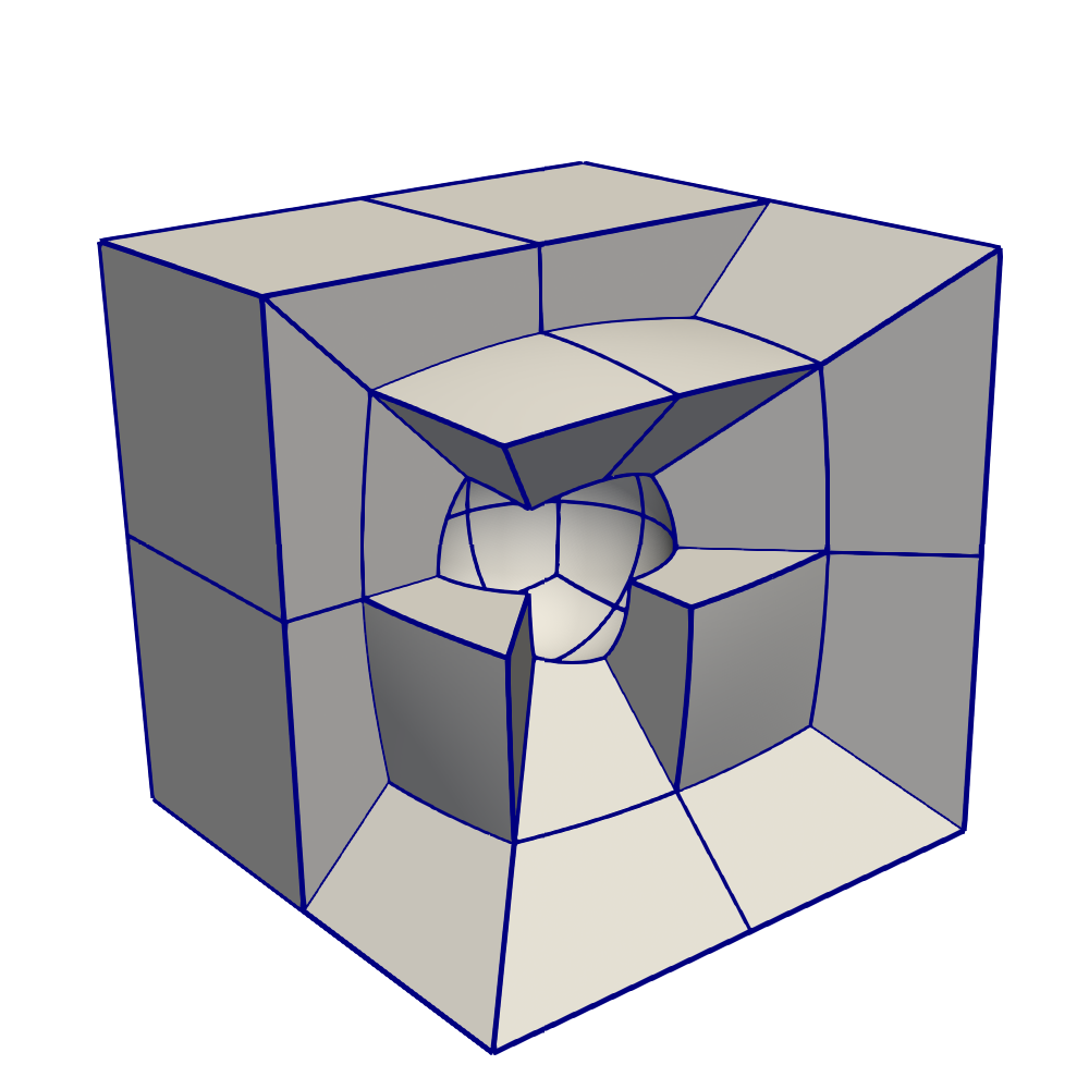
Figure 4: Cubic domain with a spherical hole and curved cells

In Table 2, we report the ratio of the $L^{2}$ norm of the errors at a final time $t_{f}=1$ using solution polynomials of degree $p=2,3,4,7,9$. Both interior and boundary faces describing the spherical geometry are approximated with polynomials of the same order. We observe that $92\%$ of the ratios are equal to or greater than one. In this case, where the mesh is less distorted, the maximum improvement is approximately $10\%$. The ratios highlighted in red deviate from one by at most $0.01\%$.

	$\rho$	$\mathcal{U}_{1}$	$\mathcal{U}_{2}$	$\mathcal{U}_{3}$	$\mathcal{T}$
$p=2$	green!25 1.094	red!25 0.999	red!25 0.999	green!25 1.139	green!25 1.093
$p=3$	green!25 1.018	green!25 1.019	green!25 1.019	green!25 1.007	green!25 1.024
$p=4$	green!25 1.057	green!25 1.002	green!25 1.002	green!25 1.028	green!25 1.016
$p=7$	green!25 1.041	green!25 1.014	green!25 1.014	green!25 1.039	green!25 1.023
$p=9$	green!25 1.029	green!25 1.011	green!25 1.011	green!25 1.017	green!25 1.022

Table 2: Ratio of the $L^{2}$-norm of the errors (Thomas and Lombard [35] vs. optimized): propagation of the isentropic vortex in a cubic domain with a spherical hole and geometrically high order cells.

5.2 Viscous shock

Next, we study the propagation of a viscous shock using the compressible Navier–Stokes equations. We assume a planar shock propagating along the $x_{1}$ coordinate direction with a Prandtl number of $Pr=3/4$. The exact solution of this problem is known; the momentum $\mathcal{V}(x_{1})$ satisfies the ordinary differential equation

$$\begin{split}&\alpha\mathcal{V}\frac{\partial\mathcal{V}}{\partial x_{1}}-(\mathcal{V}-1)(\mathcal{V}-\mathcal{V}_{f})=0,\qquad-\infty\leq x_{1}\leq+\infty.\end{split}$$

Assuming that the center of the viscous shock is located at $x_{1}=0$, the implicit solution of the former equation is

$$x_{1}-\frac{1}{2}\alpha\left(\log\left|(\mathcal{V}(x_{1})-1)(\mathcal{V}(x_{1})-\mathcal{V}_{f})\right|+\frac{1+\mathcal{V}_{f}}{1-\mathcal{V}_{f}}\log\left|\frac{\mathcal{V}(x_{1})-1}{\mathcal{V}(x_{1})-\mathcal{V}_{f}}\right|\right)=0,$$ (36)

where

$$\mathcal{V}_{f}=\frac{\mathcal{U}_{L}}{\mathcal{U}_{R}},\qquad\alpha=\frac{2\gamma}{\gamma+1}\frac{\,\mu}{Pr\dot{\mathcal{M}}}.$$ (37)

Here $\mathcal{U}_{L/R}$ are known velocities to the left and right of the shock at $-\infty$ and $+\infty$, respectively, $\dot{\mathcal{M}}$ is the constant mass flow across the shock, $Pr$ is the Prandtl number, and $\mu$ is the dynamic viscosity. The mass and total enthalpy are constant across the shock, and the momentum and energy equations become redundant.

For our tests, $\mathcal{V}$ is computed from Equation (36) to machine precision using bisection. The moving shock solution is obtained by applying a uniform translation to the above solution. The shock is located at the center of the domain at $t=0$, and the following values are used: $M_{\infty}=2.5$, $Re_{\infty}=10$, and $\gamma=1.4$. The boundary conditions are prescribed by penalizing the numerical solution against the exact solution. The analytical solution is also used to furnish data for the initial conditions.

We investigate the $L^{2}$ norm of the error for the same meshes discussed for the isentropic vortex configurations; the simulations are stopped at a final time $t_{f}=5$.

5.2.1 Cubic domain with geometrically high order perturbed cells

We consider solution polynomials of degree $p=1,2,3,4,7,15$ and four values of the perturbation parameter, i.e., $\eta=0.25,0.5,0.75,1$. In Table 3, we report the ratio of the $L^{2}$ norm of the errors of the primitive variables computed using the metrics of Thomas and Lombard [35] and the optimization algorithm presented herein. We observe that $80\%$ of the ratios are equal to or greater than one, where in some cases the improvement is more than $40\%$. For the cases where the ratio is highlighted in red, the maximum deviation from one is approximately $1.6\%$. Furthermore, we note that by increasing the degree of the solution polynomial the ratio of the two error norms converges to one.

	$\rho$
$\eta$	$0.25$	$0.5$	$0.75$	$1.0$
$p=1$	green!25 1.000	green!25 1.000	green!25 1.000	green!25 1.000
$p=2$	green!25 1.213	green!25 1.536	green!25 1.776	green!25 1.951
$p=3$	green!25 1.027	green!25 1.055	green!25 1.078	green!25 1.098
$p=4$	green!25 1.050	green!25 1.072	green!25 1.058	green!25 1.032
$p=7$	red!25 0.996	red!25 0.995	red!25 0.996	red!25 0.999
$p=9$	green!25 1.000	green!25 1.000	green!25 1.000	green!25 1.000
$p=15$	green!25 1.000	green!25 1.000	green!25 1.000	green!25 1.000

(a)

	$\mathcal{U}_{1}$
$\eta$	$0.25$	$0.5$	$0.75$	$1.0$
$p=1$	green!25 1.000	green!25 1.000	green!25 1.000	green!25 1.000
$p=2$	green!25 1.187	green!25 1.418	green!25 1.546	green!25 1.623
$p=3$	green!25 1.034	green!25 1.054	green!25 1.059	green!25 1.067
$p=4$	green!25 1.098	green!25 1.121	green!25 1.114	green!25 1.098
$p=7$	red!25 0.992	red!25 0.986	red!25 0.984	red!25 0.985
$p=9$	red!25 0.998	red!25 0.998	red!25 0.998	red!25 0.999
$p=15$	green!25 1.000	green!25 1.000	green!25 1.000	green!25 1.000

(b)

	$\mathcal{U}_{2}$
$\eta$	$0.25$	$0.5$	$0.75$	$1.0$
$p=1$	green!25 1.000	green!25 1.000	green!25 1.000	green!25 1.000
$p=2$	green!25 1.187	green!25 1.418	green!25 1.546	green!25 1.623
$p=3$	green!25 1.034	green!25 1.054	green!25 1.059	green!25 1.067
$p=4$	green!25 1.098	green!25 1.121	green!25 1.114	green!25 1.098
$p=7$	red!25 0.992	red!25 0.986	red!25 0.984	red!25 0.985
$p=9$	red!25 0.998	red!25 0.998	red!25 0.998	red!25 0.999
$p=15$	green!25 1.000	green!25 1.000	green!25 1.000	green!25 1.000

(c)

	$\mathcal{U}_{3}$
$\eta$	$0.25$	$0.5$	$0.75$	$1.0$
$p=1$	green!25 1.000	green!25 1.000	green!25 1.000	green!25 1.000
$p=2$	green!25 1.187	green!25 1.418	green!25 1.546	green!25 1.623
$p=3$	green!25 1.034	green!25 1.054	green!25 1.059	green!25 1.067
$p=4$	green!25 1.098	green!25 1.121	green!25 1.114	green!25 1.098
$p=7$	red!25 0.992	red!25 0.986	red!25 0.984	red!25 0.985
$p=9$	red!25 0.998	red!25 0.998	red!25 0.998	red!25 0.999
$p=15$	green!25 1.000	green!25 1.000	green!25 1.000	green!25 1.000

(d)

	$\mathcal{T}$
$\eta$	$0.25$	$0.5$	$0.75$	$1.0$
$p=1$	green!25 1.000	green!25 1.000	green!25 1.000	green!25 1.000
$p=2$	green!25 1.227	green!25 1.467	green!25 1.568	green!25 1.633
$p=3$	green!25 1.105	green!25 1.182	green!25 1.226	green!25 1.262
$p=4$	green!25 1.203	green!25 1.208	green!25 1.184	green!25 1.161
$p=7$	red!25 0.996	green!25 1.011	green!25 1.020	green!25 1.023
$p=9$	green!25 1.002	green!25 1.006	green!25 1.006	green!25 1.005
$p=15$	green!25 1.000	green!25 1.000	green!25 1.000	green!25 1.000

(e)

Table 3: Ratio of the $L^{2}$-norm of the errors (Thomas and Lombard [35] vs. optimized): propagation of the viscous shock in a cubic domain with geometrically high order perturbed cells.

5.2.2 Cubic domain with a spherical hole and geometrically high order cells

In Table 4, we report the ratio of the $L^{2}$ norm of the errors of the primitive variables. Solution polynomials of degree $p=2,3,4,7,9$ are used. Boundary faces describing the spherical geometry as well as internal curved interfaces are approximated with polynomials of degree $p$. We observe that $70\%$ of the ratios are equal to or greater than one with a maximum gain of $5\%$ for the solution computed with the optimized metrics. The ratio highlighted in red has a maximum deviation from one of just $1.9\%$.

	$\rho$	$\mathcal{U}_{1}$	$\mathcal{U}_{2}$	$\mathcal{U}_{3}$	$\mathcal{T}$
$p=2$	green!25 1.013	red!25 0.981	red!25 0.981	red!25 0.981	green!25 1.047
$p=3$	green!25 1.000	red!25 0.997	red!25 0.997	red!25 0.997	red!25 0.996
$p=4$	green!25 1.001	green!25 1.000	green!25 1.000	green!25 1.000	green!25 1.005
$p=7$	green!25 1.000	green!25 1.000	green!25 1.000	green!25 1.000	green!25 1.000
$p=9$	green!25 1.000	green!25 1.000	green!25 1.000	green!25 1.000	green!25 1.000

Table 4: Ratio of the $L^{2}$ norm of the errors (Thomas and Lombard [35] vs. optimized): propagation of the viscous shock in a cubic domain with a spherical hole and geometrically high order cells.

6 Conclusion

We numerically show that optimizing the metric terms as proposed in [16, 12, 14] lead, even for conforming interfaces, to a solution whose accuracy is practically never worse and often noticeably better than the one obtained using the widely adopted Thomas and Lombard metric terms computation [35]. We also observed that by increasing the degree of the solution polynomial, the ratio of the two error norms converges to one. This indicates that the benefits of optimizing the metric terms decrease by increasing the solution polynomial degree of the spatial approximation. We conclude that the pre-processing step of optimizing the metric terms can then be used in a computational framework as a unique and viable approach for conforming and $h/p$ non-conforming interfaces. In addition, this choice greatly simplifies the solver and allows important code re-utilization. Investigating the effect of the optimized metrics on other important systems of PDEs is a future research direction.

Appendix A $L^{2}$ norm of the error: Isentropic vortex

A.1 Cubic domain with geometrically high order perturbed cells

	$\rho$
$\eta$	$0.25$	$0.5$	$0.75$	$1.0$
$p=1$	6.062e-03	6.062e-03	6.062e-03	6.062e-03
$p=2$	1.210e-03	1.888e-03	2.610e-03	3.313e-03
$p=3$	4.024e-04	7.994e-04	1.210e-03	1.633e-03
$p=4$	1.456e-04	2.982e-04	4.683e-04	6.644e-04
$p=7$	1.381e-06	4.875e-06	1.193e-05	2.398e-05
$p=9$	6.974e-08	3.724e-07	1.112e-06	2.506e-06
$p=15$	1.127e-11	1.186e-10	5.584e-10	1.847e-09

(a) Thomas and Lombard metrics [35].

	$\rho$
$\eta$	$0.25$	$0.5$	$0.75$	$1.0$
$p=1$	6.062e-03	6.062e-03	6.062e-03	6.062e-03
$p=2$	9.371e-04	1.212e-03	1.625e-03	2.161e-03
$p=3$	1.427e-04	3.110e-04	5.664e-04	9.097e-04
$p=4$	4.993e-05	1.273e-04	2.488e-04	4.199e-04
$p=7$	1.026e-06	4.388e-06	1.135e-05	2.338e-05
$p=9$	6.660e-08	3.677e-07	1.109e-06	2.511e-06
$p=15$	1.110e-11	1.186e-10	5.585e-10	1.847e-09

(b) Optimized metrics.

Table 5: $L^{2}$ error norm of the density: propagation of the isentropic vortex in a cubic domain with geometrically high order perturbed cells.

	$\mathcal{U}_{1}$
$\eta$	$0.25$	$0.5$	$0.75$	$1.0$
$p=1$	1.694e-02	1.694e-02	1.694e-02	1.694e-02
$p=2$	4.635e-03	7.990e-03	1.170e-02	1.562e-02
$p=3$	1.146e-03	2.393e-03	4.003e-03	6.003e-03
$p=4$	3.589e-04	8.494e-04	1.563e-03	2.534e-03
$p=7$	6.144e-06	2.445e-05	5.768e-05	1.117e-04
$p=9$	3.691e-07	1.673e-06	4.549e-06	1.022e-05
$p=15$	2.608e-11	3.024e-10	1.685e-09	6.562e-09

(a) Thomas and Lombard metrics [35].

	$\mathcal{U}_{1}$
$\eta$	$0.25$	$0.5$	$0.75$	$1.0$
$p=1$	1.694e-02	1.694e-02	1.694e-02	1.694e-02
$p=2$	3.121e-03	4.322e-03	6.376e-03	9.074e-03
$p=3$	6.269e-04	1.348e-03	2.537e-03	4.156e-03
$p=4$	2.267e-04	6.441e-04	1.295e-03	2.180e-03
$p=7$	5.886e-06	2.364e-05	5.597e-05	1.096e-04
$p=9$	3.659e-07	1.663e-06	4.543e-06	1.027e-05
$p=15$	2.606e-11	3.024e-10	1.685e-09	6.562e-09

(b) Optimized metrics.

Table 6: $L^{2}$ error norm of the velocity component in $x_{1}$: propagation of the isentropic vortex in a cubic domain with geometrically high order perturbed cells.

	$\mathcal{U}_{2}$
$\eta$	$0.25$	$0.5$	$0.75$	$1.0$
$p=1$	1.694e-02	1.694e-02	1.694e-02	1.694e-02
$p=2$	4.731e-03	8.215e-03	1.207e-02	1.614e-02
$p=3$	1.279e-03	2.590e-03	4.183e-03	6.158e-03
$p=4$	4.159e-04	9.325e-04	1.638e-03	2.595e-03
$p=7$	6.125e-06	2.372e-05	5.962e-05	1.215e-04
$p=9$	3.406e-07	1.738e-06	5.138e-06	1.162e-05
$p=15$	4.037e-11	4.686e-10	2.518e-09	9.149e-09

(a) Thomas and Lombard metrics [35].

	$\mathcal{U}_{2}$
$\eta$	$0.25$	$0.5$	$0.75$	$1.0$
$p=1$	1.694e-02	1.694e-02	1.694e-02	1.694e-02
$p=2$	3.065e-03	4.053e-03	5.807e-03	8.212e-03
$p=3$	7.021e-04	1.433e-03	2.612e-03	4.287e-03
$p=4$	2.107e-04	5.995e-04	1.229e-03	2.107e-03
$p=7$	5.799e-06	2.285e-05	5.818e-05	1.195e-04
$p=9$	3.349e-07	1.730e-06	5.148e-06	1.168e-05
$p=15$	4.039e-11	4.689e-10	2.519e-09	9.151e-09

(b) Optimized metrics.

Table 7: $L^{2}$ error norm of the velocity component in $x_{2}$: propagation of the isentropic vortex in a cubic domain with geometrically high order perturbed cells.

	$\mathcal{U}_{3}$
$\eta$	$0.25$	$0.5$	$0.75$	$1.0$
$p=1$	7.813e-03	7.813e-03	7.813e-03	7.813e-03
$p=2$	2.439e-03	4.468e-03	6.427e-03	8.357e-03
$p=3$	1.272e-03	2.577e-03	4.051e-03	5.800e-03
$p=4$	4.767e-04	1.009e-03	1.648e-03	2.448e-03
$p=7$	5.851e-06	2.218e-05	5.467e-05	1.102e-04
$p=9$	3.187e-07	1.746e-06	5.195e-06	1.180e-05
$p=15$	4.049e-11	4.332e-10	2.107e-09	7.318e-09

(a) Thomas and Lombard metrics [35].

	$\mathcal{U}_{3}$
$\eta$	$0.25$	$0.5$	$0.75$	$1.0$
$p=1$	7.813e-03	7.813e-03	7.813e-03	7.813e-03
$p=2$	1.786e-03	3.145e-03	5.057e-03	7.393e-03
$p=3$	5.711e-04	1.393e-03	2.597e-03	4.170e-03
$p=4$	2.155e-04	6.000e-04	1.195e-03	2.012e-03
$p=7$	4.900e-06	2.065e-05	5.241e-05	1.073e-04
$p=9$	3.089e-07	1.729e-06	5.191e-06	1.183e-05
$p=15$	4.049e-11	4.333e-10	2.107e-09	7.319e-09

(b) Optimized metrics.

Table 8: $L^{2}$ error norm of the velocity component in $x_{3}$: propagation of the isentropic vortex in a cubic domain with geometrically high order perturbed cells.

	$\mathcal{T}$
$\eta$	$0.25$	$0.5$	$0.75$	$1.0$
$p=1$	3.038e-03	3.038e-03	3.038e-03	3.038e-03
$p=2$	5.380e-04	8.319e-04	1.181e-03	1.562e-03
$p=3$	1.838e-04	3.624e-04	5.555e-04	7.683e-04
$p=4$	6.521e-05	1.342e-04	2.139e-04	3.095e-04
$p=7$	6.432e-07	2.329e-06	5.680e-06	1.130e-05
$p=9$	3.623e-08	1.929e-07	5.686e-07	1.277e-06
$p=15$	8.778e-12	9.668e-11	4.670e-10	1.575e-09

(a) Thomas and Lombard metrics [35].

	$\mathcal{T}$
$\eta$	$0.25$	$0.5$	$0.75$	$1.0$
$p=1$	3.038e-03	3.038e-03	3.038e-03	3.038e-03
$p=2$	4.350e-04	5.648e-04	7.632e-04	1.022e-03
$p=3$	7.775e-05	1.489e-04	2.584e-04	4.058e-04
$p=4$	2.859e-05	6.747e-05	1.265e-04	2.094e-04
$p=7$	4.951e-07	2.121e-06	5.425e-06	1.102e-05
$p=9$	3.506e-08	1.910e-07	5.669e-07	1.278e-06
$p=15$	8.735e-12	9.668e-11	4.670e-10	1.575e-09

(b) Optimized metrics.

Table 9: $L^{2}$ error norm of the temperature: propagation of the isentropic vortex in a cubic domain with geometrically high order perturbed cells.

A.2 Cubic domain with a spherical hole and geometrically high order cells

	$\rho$	$\mathcal{U}_{1}$	$\mathcal{U}_{2}$	$\mathcal{U}_{3}$	$\mathcal{T}$
$p=2$	1.264e-03	6.661e-03	6.661e-03	3.507e-03	5.725e-04
$p=3$	1.293e-04	6.434e-04	6.434e-04	6.700e-04	5.397e-05
$p=4$	2.193e-05	1.167e-04	1.167e-04	6.360e-05	1.208e-05
$p=7$	5.360e-08	5.091e-07	5.091e-07	2.593e-07	2.957e-08
$p=9$	1.608e-09	1.762e-08	1.762e-08	7.390e-09	7.782e-10

Table 10: $L^{2}$-norm of the errors for the Thomas and Lombard metrics [35]: propagation of the isentropic vortex in a cubic domain with a spherical hole and geometrically high order cells.

	$\rho$	$\mathcal{U}_{1}$	$\mathcal{U}_{2}$	$\mathcal{U}_{3}$	$\mathcal{T}$
$p=2$	1.155e-03	6.665e-03	6.665e-03	3.079e-03	5.236e-04
$p=3$	1.270e-04	6.311e-04	6.311e-04	6.653e-04	5.268e-05
$p=4$	2.074e-05	1.164e-04	1.164e-04	6.187e-05	1.189e-05
$p=7$	5.149e-08	5.019e-07	5.019e-07	2.496e-07	2.889e-08
$p=9$	1.562e-09	1.742e-08	1.742e-08	7.268e-09	7.614e-10

Table 11: $L^{2}$-norm of the errors for the optimized metrics: propagation of the isentropic vortex in a cubic domain with a spherical hole and geometrically high order cells.

Appendix B Numerical results: Viscous shock

B.1 Cubic domain with geometrically high order perturbed cells

	$\rho$
$\eta$	$0.25$	$0.5$	$0.75$	$1.0$
$p=1$	3.795e-02	3.795e-02	3.795e-02	3.795e-02
$p=2$	1.673e-02	2.486e-02	3.384e-02	4.267e-02
$p=3$	4.121e-03	6.915e-03	9.867e-03	1.282e-02
$p=4$	1.956e-03	3.350e-03	5.118e-03	7.082e-03
$p=7$	1.244e-04	2.699e-04	4.902e-04	7.852e-04
$p=9$	2.216e-05	5.799e-05	1.192e-04	2.118e-04
$p=15$	1.393e-07	6.844e-07	2.249e-06	5.832e-06

(a) Thomas and Lombard metrics [35].

	$\rho$
$\eta$	$0.25$	$0.5$	$0.75$	$1.0$
$p=1$	3.795e-02	3.795e-02	3.795e-02	3.795e-02
$p=2$	1.380e-02	1.618e-02	1.906e-02	2.187e-02
$p=3$	4.014e-03	6.554e-03	9.156e-03	1.168e-02
$p=4$	1.863e-03	3.125e-03	4.840e-03	6.862e-03
$p=7$	1.249e-04	2.713e-04	4.919e-04	7.860e-04
$p=9$	2.217e-05	5.800e-05	1.192e-04	2.117e-04
$p=15$	1.393e-07	6.844e-07	2.249e-06	5.832e-06

(b) Optimized metrics.

Table 12: $L^{2}$ error norm of the density: propagation of the viscous shock in a cubic domain with geometrically high order perturbed cells.

	$\mathcal{U}_{1}$
$\eta$	$0.25$	$0.5$	$0.75$	$1.0$
$p=1$	1.030e-02	1.030e-02	1.030e-02	1.030e-02
$p=2$	2.406e-03	3.587e-03	4.915e-03	6.335e-03
$p=3$	6.446e-04	9.659e-04	1.346e-03	1.769e-03
$p=4$	2.330e-04	4.228e-04	6.496e-04	9.159e-04
$p=7$	1.023e-05	2.333e-05	4.458e-05	7.568e-05
$p=9$	1.529e-06	4.296e-06	9.478e-06	1.777e-05
$p=15$	6.950e-09	3.633e-08	1.228e-07	3.236e-07

(a) Thomas and Lombard metrics [35].

	$\mathcal{U}_{1}$
$\eta$	$0.25$	$0.5$	$0.75$	$1.0$
$p=1$	1.030e-02	1.030e-02	1.030e-02	1.030e-02
$p=2$	2.027e-03	2.530e-03	3.180e-03	3.904e-03
$p=3$	6.236e-04	9.166e-04	1.271e-03	1.658e-03
$p=4$	2.122e-04	3.773e-04	5.832e-04	8.344e-04
$p=7$	1.031e-05	2.366e-05	4.530e-05	7.687e-05
$p=9$	1.531e-06	4.306e-06	9.496e-06	1.779e-05
$p=15$	6.950e-09	3.633e-08	1.228e-07	3.236e-07

(b) Optimized metrics.

Table 13: $L^{2}$ error norm of the velocity component in $x_{1}$: propagation of the viscous shock in a cubic domain with geometrically high order perturbed cells.

	$\mathcal{U}_{2}$
$\eta$	$0.25$	$0.5$	$0.75$	$1.0$
$p=1$	1.030e-02	1.030e-02	1.030e-02	1.030e-02
$p=2$	2.406e-03	3.587e-03	4.915e-03	6.335e-03
$p=3$	6.446e-04	9.659e-04	1.346e-03	1.769e-03
$p=4$	2.330e-04	4.228e-04	6.496e-04	9.159e-04
$p=7$	1.023e-05	2.333e-05	4.458e-05	7.568e-05
$p=9$	1.529e-06	4.296e-06	9.478e-06	1.777e-05
$p=15$	6.950e-09	3.633e-08	1.228e-07	3.236e-07

(a) Thomas and Lombard metrics [35].

	$\mathcal{U}_{2}$
$\eta$	$0.25$	$0.5$	$0.75$	$1.0$
$p=1$	1.030e-02	1.030e-02	1.030e-02	1.030e-02
$p=2$	2.027e-03	2.530e-03	3.180e-03	3.904e-03
$p=3$	6.236e-04	9.166e-04	1.271e-03	1.658e-03
$p=4$	2.122e-04	3.773e-04	5.832e-04	8.344e-04
$p=7$	1.031e-05	2.366e-05	4.530e-05	7.687e-05
$p=9$	1.531e-06	4.306e-06	9.496e-06	1.779e-05
$p=15$	6.950e-09	3.633e-08	1.228e-07	3.236e-07

(b) Optimized metrics.

Table 14: $L^{2}$ error norm of the velocity component in $x_{2}$: propagation of the viscous shock in a cubic domain with geometrically high order perturbed cells.

	$\mathcal{U}_{3}$
$\eta$	$0.25$	$0.5$	$0.75$	$1.0$
$p=1$	1.030e-02	1.030e-02	1.030e-02	1.030e-02
$p=2$	2.406e-03	3.587e-03	4.915e-03	6.335e-03
$p=3$	6.446e-04	9.659e-04	1.346e-03	1.769e-03
$p=4$	2.330e-04	4.228e-04	6.496e-04	9.159e-04
$p=7$	1.023e-05	2.333e-05	4.458e-05	7.568e-05
$p=9$	1.529e-06	4.296e-06	9.478e-06	1.777e-05
$p=15$	6.950e-09	3.633e-08	1.228e-07	3.236e-07

(a) Thomas and Lombard metrics [35].

	$\mathcal{U}_{3}$
$\eta$	$0.25$	$0.5$	$0.75$	$1.0$
$p=1$	1.030e-02	1.030e-02	1.030e-02	1.030e-02
$p=2$	2.027e-03	2.530e-03	3.180e-03	3.904e-03
$p=3$	6.236e-04	9.166e-04	1.271e-03	1.658e-03
$p=4$	2.122e-04	3.773e-04	5.832e-04	8.344e-04
$p=7$	1.031e-05	2.366e-05	4.530e-05	7.687e-05
$p=9$	1.531e-06	4.306e-06	9.496e-06	1.779e-05
$p=15$	6.950e-09	3.633e-08	1.228e-07	3.236e-07

(b) Optimized metrics.

Table 15: $L^{2}$ error norm of the velocity component in $x_{3}$: propagation of the viscous shock in a cubic domain with geometrically high order perturbed cells.

	$\mathcal{T}$
$\eta$	$0.25$	$0.5$	$0.75$	$1.0$
$p=1$	2.864e-02	2.864e-02	2.864e-02	2.864e-02
$p=2$	5.072e-03	8.012e-03	1.142e-02	1.530e-02
$p=3$	1.190e-03	1.982e-03	2.942e-03	4.102e-03
$p=4$	4.457e-04	8.996e-04	1.441e-03	2.090e-03
$p=7$	1.284e-05	3.472e-05	7.484e-05	1.366e-04
$p=9$	1.576e-06	5.798e-06	1.437e-05	2.818e-05
$p=15$	5.170e-09	3.352e-08	1.342e-07	4.256e-07

(a) Thomas and Lombard metrics [35].

	$\mathcal{T}$
$\eta$	$0.25$	$0.5$	$0.75$	$1.0$
$p=1$	2.864e-02	2.864e-02	2.864e-02	2.864e-02
$p=2$	4.133e-03	5.462e-03	7.282e-03	9.373e-03
$p=3$	1.077e-03	1.677e-03	2.400e-03	3.250e-03
$p=4$	3.704e-04	7.448e-04	1.218e-03	1.801e-03
$p=7$	1.289e-05	3.435e-05	7.336e-05	1.336e-04
$p=9$	1.573e-06	5.764e-06	1.428e-05	2.803e-05
$p=15$	5.170e-09	3.352e-08	1.342e-07	4.256e-07

(b) Optimized metrics.

Table 16: $L^{2}$ error norm of the temperature: propagation of the viscous shock in a cubic domain with geometrically high order perturbed cells.

B.2 Cubic domain with a spherical hole and geometrically high order cells

	$\rho$	$\mathcal{U}_{1}$	$\mathcal{U}_{2}$	$\mathcal{U}_{3}$	$\mathcal{T}$
$p=2$	1.184e-02	1.519e-03	1.519e-03	1.519e-03	4.269e-03
$p=3$	4.587e-03	4.340e-04	4.340e-04	4.340e-04	1.057e-03
$p=4$	1.820e-03	1.340e-04	1.340e-04	1.340e-04	3.222e-04
$p=7$	1.370e-04	9.784e-06	9.784e-06	9.784e-06	1.054e-05
$p=9$	2.176e-05	1.854e-06	1.854e-06	1.854e-06	1.729e-06

Table 17: $L^{2}$-norm of the errors for the Thomas and Lombard metrics [35]: propagation of the viscous shock in a cubic domain with a spherical hole and geometrically high order cells.

	$\rho$	$\mathcal{U}_{1}$	$\mathcal{U}_{2}$	$\mathcal{U}_{3}$	$\mathcal{T}$
$p=2$	1.169e-02	1.548e-03	1.548e-03	1.548e-03	4.076e-03
$p=3$	4.586e-03	4.352e-04	4.352e-04	4.352e-04	1.062e-03
$p=4$	1.817e-03	1.340e-04	1.340e-04	1.340e-04	3.205e-04
$p=7$	1.370e-04	9.784e-06	9.784e-06	9.784e-06	1.054e-05
$p=9$	2.176e-05	1.854e-06	1.854e-06	1.854e-06	1.729e-06

Table 18: $L^{2}$-norm of the errors for the optimized metrics: propagation of the viscous shock in a cubic domain with a spherical hole and geometrically high order cells.

References

• [1] R. Abgrall and M. Ricchiuto, High order methods for CFD, in Encyclopedia of Computational Mechanics, John Wiley & Sons, Ltd, 2017.
• [2] S. Abhyankar, J. Brown, E. M. Constantinescu, D. Ghosh, B. F. Smith, and H. Zhang, PETSc/TS: A modern scalable ODE/DAE solver library, arXiv preprint arXiv:1806.01437, (2018).
• [3] S. Balay, S. Abhyankar, M. F. Adams, J. Brown, P. Brune, K. Buschelman, L. Dalcin, A. Dener, V. Eijkhout, W. D. Gropp, D. Karpeyev, D. Kaushik, M. G. Knepley, D. A. May, L. C. McInnes, R. T. Mills, T. Munson, K. Rupp, P. Sanan, B. F. Smith, S. Zampini, H. Zhang, and H. Zhang, PETSc users manual, Tech. Rep. ANL-95/11 - Revision 3.11, Argonne National Laboratory, 2019.
• [4] P. Bogacki and L. Shampine, A 3(2) pair of runge - kutta formulas, Applied Mathematics Letters, 2 (1989), pp. 321 – 325.
• [5] M. Carpenter, T. Fisher, E. Nielsen, and S. Frankel, Entropy stable spectral collocation schemes for the Navier–Stokes equations: Discontinuous interfaces, SIAM Journal on Scientific Computing, 36 (2014), pp. B835–B867.
• [6] M. H. Carpenter, M. Parsani, T. C. Fisher, and E. J. Nielsen, Entropy stable staggered grid spectral collocation for the Burgers’ and the compressible Navier–Stokes equations, NASA TM-2015-218990, (2015).
• [7] M. H. Carpenter, M. Parsani, E. J. Nielsen, and T. C. Fisher, Towards an entropy stable spectral element framework for computational fluid dynamics, in 54th AIAA Aerospace Sciences Meeting, AIAA 2016-1058, American Institute of Aeronautics and Astronautics (AIAA), 2016.
• [8] P. Chandrashekar, Kinetic energy preserving and entropy stable finite volume schemes for compressible Euler and Navier–Stokes equations, Communications in Computational Physics, 14 (2013), pp. 1252–1286.
• [9] J. Crean, J. E. Hicken, D. C. D. R. Fernández, D. W. Zingg, and M. H. Carpenter, Entropy-stable summation-by-parts discretization of the Euler equations on general curved elements, Journal of Computational Physics, 356 (2018), pp. 410 – 438.
• [10] C. M. Dafermos, Hyperbolic conservation laws in continuum physics, Springer-Verlag, Berlin, 2010.
• [11] D. C. Del Rey Fernández, P. D. Boom, and D. W. Zingg, A generalized framework for nodal first derivative summation-by-parts operators, Journal of Computational Physics, 266 (2014), pp. 214–239.
• [12] D. C. Del Rey Fernández, M. H. Carpenter, L. Dalcin, L. Fredrich, A. R. Winters, G. J. Gassner, S. Zampini, and M. Parsani, Entropy stable $p-$nonconforming discretizations with the summation-by-parts property for the compressible Euler equations, Submitted to SIAM Journal of Scientific Computing, (2019).
• [13] D. C. Del Rey Fernández, M. H. Carpenter, L. Dalcin, L. Fredrich, A. R. Winters, G. J. Gassner, S. Zampini, and M. Parsani, Entropy stable $p-$nonconforming discretizations with the summation-by-parts property for the compressible Navier–Stokes equations, Submitted to Computer & Fluids, (2019).
• [14] D. C. Del Rey Fernández, M. H. Carpenter, L. Dalcin, S. Zampini, and M. Parsani, Entropy stable $h/p$ non-conforming discretization with the summation-by-parts property for the compressible Euler and Navier–Stokes equations, Submitted to SN Partial Differential Equations and Applications (2019).
• [15] D. C. Del Rey Fernández, J. E. Hicken, and D. W. Zingg, Review of summation-by-parts operators with simultaneous approximation terms for the numerical solution of partial differential equations, Computers & Fluids, 95 (2014), pp. 171–196.
• [16] D. C. Fernández, M. H. Carpenter, L. Dalcin, L. Fredrich, D. Rojas, A. R. Winters, G. J. Gassner, S. Zampini, and M. Parsani, Entropy stable non-conforming discretizations with the summation-by-parts property for curvilinear coordinates, NASA TM-2019-, (2019).
• [17] T. C. Fisher, High-order $L^{2}$ stable multi-domain finite difference method for compressible flows, PhD thesis, Purdue University, 2012.
• [18] T. C. Fisher and M. H. Carpenter, High-order entropy stable finite difference schemes for nonlinear conservation laws: finite domains, Journal of Computational Physics, 252 (2013), pp. 518–557.
• [19] L. Friedrich, A. R. Winters, D. C. Del Rey Fernández, G. J. Gassner, M. Parsani, and M. H. Carpenter, An entropy stable h/p non-conforming discontinuous Galerkin method with the summation-by-parts property, Journal of Scientific Computing, 77 (2018).
• [20] G. J. Gassner, A. R. Winters, and D. A. Kopriva, Split form nodal discontinuous Galerkin schemes with summation-by-parts property for the compressible Euler equations, Journal of Computational Physics, 327 (2016), pp. 39–66.
• [21] G. J. Gassner, A. R. Winters, and D. A. Kopriva, A well balanced and entropy conservative discontinuous Galerkin spectral element method for the shallow water equations, Applied Mathematics and Computation, 272 (2016), pp. 291 – 308. Recent Advances in Numerical Methods for Hyperbolic Partial Differential Equations.
• [22] J. S. Hesthaven and T. Warburton, Nodal discontinuous Galerkin methods: Algorithms, analysis, and applications, Texts in Applied Mathematics, Springer, 2008.
• [23] C. Hirsch, Numerical computation of internal and external flows. Vol. 2 - Computational methods for inviscid and viscous flows, 1990.
• [24] H. Huynh, Z. Wang, and P. Vincent, High-order methods for computational fluid dynamics: A brief review of compact differential formulations on unstructured grids, Computers & Fluids, 98 (2014), pp. 209 – 220.
• [25] M. G. Knepley and D. A. Karpeev, Mesh algorithms for PDE with Sieve I: Mesh distribution, Scientific Programming, 17 (2009), pp. 215–230.
• [26] M. Parsani, M. Carpenter, T. Fisher, and E. Nielsen, Entropy stable staggered grid discontinuous spectral collocation methods of any order for the compressible Navier–Stokes equations, SIAM Journal on Scientific Computing, 38 (2016), pp. A3129–A3162.
• [27] M. Parsani, M. H. Carpenter, and E. J. Nielsen, Entropy stable discontinuous interfaces coupling for the three-dimensional compressible Navier–Stokes equations, Journal of Computational Physics, 290 (2015), pp. 132–138.
• [28]  , Entropy stable wall boundary conditions for the three-dimensional compressible Navier–Stokes equations, Journal of Computational Physics, 292 (2015), pp. 88–113.
• [29] M. Parsani, M. H. Carpenter, and E. J. Nielsen, Entropy stable wall boundary conditions for the three-dimensional compressible Navier–Stokes equations, Journal of Computational Physics, 292 (2015), pp. 88–113.
• [30] W. Pazner and P.-O. Persson, Analysis and entropy stability of the line-based discontinuous Galerkin method, Journal of Scientific Computing, 80 (2019), pp. 376–402.
• [31] D. Rojas, R. Boukharfane, L. Dalcin, D. C. Del Rey Fernández, H. Ranocha, D. E. Keyes, and M. Parsani, On the robustness and performance of entropy stable discontinuous collocation methods for the compressible navie-stokes equations, (2019). Submitted to Journal of Computational Physics.
• [32] G. Söderlind, Digital filters in adaptive time-stepping, ACM Transactions on Mathematical Software, 29 (2003), pp. 1–26.
• [33] G. Söderlind and L. Wang, Adaptive time-stepping and computational stability, Journal of Computational and Applied Mathematics, 185 (2006), pp. 225–243.
• [34] M. Svärd and J. Nordström, Review of summation-by-parts schemes for initial-boundary-value-problems, Journal of Computational Physics, 268 (2014), pp. 17–38.
• [35] P. D. Thomas and C. K. Lombard, Geometric conservation law and its application to flow computations on moving grids, AIAA Journal, 17 (1979), pp. 1030–1037.
• [36] J. F. Thompson, Z. U. Warsi, and C. W. Mastin, Boundary-fitted coordinate systems for numerical solution of partial differential equations - a review, Journal of Computational Physics, 47 (1982), pp. 1 – 108.
• [37] M. Vinokur, Conservation equations of gasdynamics in curvilinear coordinate systems, Journal of Computational Physics, 14 (1974), pp. 105 – 125.
• [38] M. Vinokur, An analysis of finite-difference and finite-volume formulations of conservation laws, Journal of Computational Physics, 81 (1989), pp. 1 – 52.
• [39] M. Vinokur and H. C. Yee, Extension of efficient low dissipation high order schemes for $3$-d curvilinear moving grids, in Frontiers of Computational Fluid Dynamics, D. A. Caughey and M. Hafez, eds., World Scientific Publishing Company, 2002, pp. 129–164.
• [40] Z. Wang, K. Fidkowski, R. Abgrall, F. Bassi, D. Caraeni, A. Cary, H. Deconinck, R. Hartmann, K. Hillewaert, H. Huynh, N. Kroll, G. May, P.-O. Persson, B. Leer, and M. Visbal, High-order cfd methods: current status and perspective, International Journal for Numerical Methods in Fluids, 72 (2012), pp. 811–845.
• [41] J. Zhu, X. Zhong, C.-W. Shu, and J. Qiu, Runge–kutta discontinuous Galerkin method using a new type of WENO limiters on unstructured meshes, Journal of Computational Physics, 248 (2013), pp. 200 – 220.