Bayesian Active Learning for Structured Output Design

Abstract

In this paper, we propose an active learning method for an inverse problem that aims to find an input that achieves a desired structured-output. The proposed method provides new acquisition functions for minimizing the error between the desired structured-output and the prediction of a Gaussian process model, by effectively incorporating the correlation between multiple outputs of the underlying multi-valued black box output functions. The effectiveness of the proposed method is verified by applying it to two synthetic shape search problem and real data. In the real data experiment, we tackle the input parameter search which achieves the desired crystal growth rate in silicon carbide (SiC) crystal growth modeling, that is a problem of materials informatics.

1 Introduction

Let us consider the problem of finding ${\bm{x}}_{0}\in\mathcal{X}$ from given ${\bm{y}}_{0}\in\mathcal{Y}$ where ${\bm{x}}_{0}$ and ${\bm{y}}_{0}$ are corresponding input and output, i.e.,

$${\bm{y}}_{0}=f({\bm{x}}_{0}).$$

These type of problems are known as inverse problems. Inverse problems have been widely studied, especially in the field of mathematics and physics (Kirsch, 2011). Indeed, there are many such problems that arise in science, for example the problem of estimating the internal parameters of a simulator of physical phenomena. In materials science, numerical calculations using simulators are widely used to predict the results of actual experiments against unknown experimental conditions. However, there are many simulators that are not accurate (in other words, the actual experimental results and the simulator’s predicted results are different). This is presumably due to the fact that the internal parameters of the simulator are not set correctly, and the estimation accuracy could be expected to be improved by limiting the range of the internal parameters using the observed actual experimental results (Adachi et al., 2005; Daggupati et al., 2010). Such problems can be formulated as an inverse problem that involves finding the internal parameters that achieve a desired experimental result (often reffered to as a structural output or “shape"). Therefore, our goal is to solve an inverse problem, the result of which is output with the desired structure or “shape". Since, in general, physical systems are often black-box, we approach this problem in a data-driven way by utilizing the observable input-output pairs as data.

Furthermore, many scientific and engineering problems are accompanied by uncertainties for various reasons such as lack of data or noisy observations. In addition, due to realistic constraints such as the costliness of conducting experiments, it is desirable to minimize the number of observations that need to be gathered from actual experiments. Active learning (or statistical experimental design, as it is also known) (Settles, 2009) is one of the most effective machine learning methods for such problems. In particular, for black box functions such as those that often comprise physical systems, an active learning method (also known as Bayesian optimization) (Shahriari et al., 2015) that introduces a Gaussian process model into the objective function and selects the next observation point by taking into account the model uncertainty, is an approach that has been widely studied.

In this paper, we tackle the inverse problem for black-box functions which return noisy, structured-output. The proposed method is formulated as a simple error minimization algorithm for vector-valued functions. Nevertheless, the novel acquisition function that takes into account the structure of the output (i.e. the correlation between functions) can efficiently find the input that achieves a desired structured output. Figure 1 demonstrates the proposed method. We can see that the red triangle (the desired structured output) can be achieved efficiently by using the prediction of the proposed method as a guide.

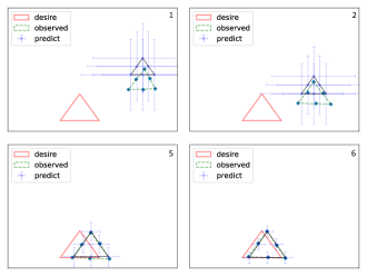
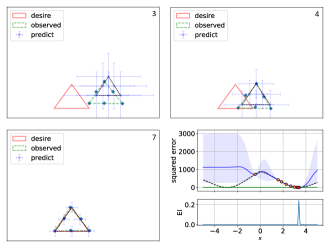
Figure 1: Demonstration of the proposed method. The search proceeds from the top left to the bottom right. The right end plot of the bottom row shows the final state of the model. We can see that based on the model (blue triangle) for the true structural output (red triangle), the next observation data (green triangle) can be selected appropriately, and the desired output can be obtained with a small number of observations. The details are explained in Section 4.

Contributions

Our contributions are summarized as follows.

• We formulate a statistical experimental design in order to find a solution of an inverse problem with structured output. We employ a Bayesian approach to handle the black-box objective function and its uncertainty.

• To handle the structured output, we design an acquisition function that considers the correlation between the components of the multidimensional output, and we proposed an input search algorithm based on Bayesian optimization.

• The effectiveness of the proposed method is verified by applying it to actual silicon carbide (SiC) crystal growth (Kusunoki et al., 2014) simulation data.

Related Work

Inverse problems can be broadly divided into two types: (i) those where the true function and output are observable but the input is not, and (ii) those where the input and output are observable but the true function is not. As an approach to the former type of problem, several methods based on Bayesian estimation (also called the Bayesian inverse problem) have been studied (Dashti and Stuart, 2016; Ardizzone et al., 2018). These approaches assume a prior distribution on the unobservable input and the goal is to estimate the posterior distribution of $y\mid x$. For the latter type of problem, we can utilize an emulator of the black-box function, learned by the observable input-output data (Conti et al., 2009; Conti and O’Hagan, 2010; Chen and Hobson, 2019). Once we have learned the emulator, we can fine-tune the input to achieve the desired output by using sensitivity analysis.

Data assimilation (Kalnay, 2003; Bannister, 2017) is a similar problem setting. This is particularly used to obtain an initial values that better explain the simulation results of time-evolving systems. In the system considered in data assimilation, in addition to the function from input ${\bm{x}}$ to output ${\bm{y}}$, the functions that describes the time evolution of ${\bm{x}}$ are also subject to modeling.

Bayesian optimization (Brochu et al., 2010; Shahriari et al., 2015), and in particular that which is based on Gaussian processes (Rasmussen and Williams, 2006), has been widely studied as a model-based active learning method for black-box functions. Bayesian optimization defines an appropriate acquisition function from a model according to the specific problem, and determines the input point for the next observation as the maximizer of this function. We consider typical acquisition functions, including optimistic ones such as the Gaussian process upper confidence bound (GPUCB), ones based on improvements such as the probability of improvement (PI) and expected improvement (EI), and ones based on information gain such as entropy search (Hennig and Schuler, 2012).

A Bayesian optimization method that has been proposed for multi-output functions with correlated structures, called multi-task Bayesian optimization (Swersky et al., 2013), is based on multi-output Gaussian processes (Bonilla et al., 2008). Multi-output Gaussian processes can appropriately model the multiple output function with a specific structure, by constructing a covariance function of the Gaussian processes from the input similarity matrix and the output similarity matrix. This method will be explained in detail in Section 2. Note that although in (Uhrenholt and Jensen, 2019), a Bayesian optimization algorithm for estimating target vector-valued output has been proposed, the structure of the output was ignored in their work.

The rest of the paper is organized as follows. In Section 2, we explain the problem setup and give some definitions. Section 3 provides an explanation of the proposed method. The overall active learning algorithm and two acquisition functions are also outlined in this section. In Section 4 we show our experimental results using both synthetic and real datasets, in order to demonstrate the effectiveness of the proposed method.

2 Preliminaries

2.1 Problem Setup

Let $\mathcal{X}\subset\mathbb{R}^{d}$ and $\mathcal{Y}\subset\mathbb{R}^{M}$ be input and output spaces, respectively. For a multiple output black-box objective function $f:\mathcal{X}\rightarrow\mathcal{Y}$, consider the task of searching for an input ${\bm{x}}_{0}=(x_{0,1},...,x_{0,d})\in\mathcal{X}$ corresponding to a given desired output ${\bm{f}}_{0}=(f_{0,1},...,f_{0,M})=(f_{1}({\bm{x}}_{0}),...,f_{M}({\bm{x}}_{0}))\in\mathcal{Y}$, where $f_{m}$, $m=1,...,M$ are scalar-valued functions corresponding to $m$-th element of $f$. Here we want to find ${\bm{x}}_{0}$ as few evaluations of $f$ as possible because $f$ can be expensive to evaluate. In addition, $f$ is generally observed with noise as

$${\bm{y}}=(y_{1},...,y_{M})=f({\bm{x}})+\bm{\varepsilon},$$

where $\bm{\varepsilon}=(\varepsilon_{1},...,\varepsilon_{M})\sim\mathcal{N}({\bm{0}},\Sigma)$ are independent Gaussian noise processes and $\Sigma$ is a diagonal matrix with elements $\sigma_{m}^{2}$, $m=1,...,M$. Therefore, we need to design a query strategy that will control the trade-off between exploration (sampling to reduce the uncertainty of $f$) and exploitation (sampling to find ${\bm{x}}_{0}$ in the region with low uncertainty). Since we are considering a function $f$ with a structured output, it would be natural to assume that $f_{1},...,f_{M}$ are correlated. To handle such a situation, $f$ is modeled by a multi-output Gaussian processes.

2.2 Gaussian Process Modeling for Structured-Output Systems

To deal with the vector-valued function $f$, we employ the multi-output Gaussian process surrogate model (Alvarez et al., 2012). For a finite number of inputs ${\bm{x}}_{1},...,{\bm{x}}_{N}$, the zero-mean Gaussian process prior is given as

$$\underbrace{\left[\begin{array}[]{c}{\bm{f}}_{1}\\ {\bm{f}}_{2}\\ {\vdots}\\ {\bm{f}}_{M}\end{array}\right]}_{={\bm{f}}}\sim\mathcal{N}\left(\left[\begin{array}[]{c}{\bm{0}}\\ {\bm{0}}\\ \vdots\\ {\bm{0}}\end{array}\right],\underbrace{\left[\begin{array}[]{cccc}{\bm{K}}_{{\bm{f}}_{1},{\bm{f}}_{1}}&\cdots&{\bm{K}}_{{\bm{f}}_{1},{\bm{f}}_{M}}\\ {\bm{K}}_{{\bm{f}}_{2},{\bm{f}}_{1}}&\cdots&{\bm{K}}_{{\bm{f}}_{2},{\bm{f}}_{M}}\\ {\vdots}&\cdots&{\vdots}\\ {\bm{K}}_{{\bm{f}}_{M},{\bm{f}}_{1}}&{\cdots}&{\bm{K}}_{{\bm{f}}_{M},{\bm{f}}_{M}}\end{array}\right]}_{={\bm{K}}}\right),$$

where ${\bm{f}}_{m}=(f_{m}({\bm{x}}_{1}),...,f_{m}({\bm{x}}_{N}))^{\top}$ is a vector-valued function corresponding to $f_{m}$ and the entries ${\bm{K}}_{{\bm{f}}_{m},{\bm{f}}_{m^{\prime}}}$ of the kernel matrix corresponding to the covariances between ${\bm{f}}_{m}$ and ${\bm{f}}_{m^{\prime}}$ which is induced by the kernel function for vector-valued output defined as

$${\bm{K}}_{m,m^{\prime}}({\bm{x}},{\bm{x}}^{\prime})=B_{m,m^{\prime}}\times k({\bm{x}},{\bm{x}}^{\prime}),$$

where $B_{m,m^{\prime}}$ describes the correlation between the function $f_{m}$ and $f_{m^{\prime}}$ ($m,m^{\prime}=1,...,M$), and $k$ is a kernel function on $\mathcal{X}$ such as Gaussian kernel. Thus, the covariance matrix ${\bm{K}}$ can be written as

$${\bm{K}} =\left(\begin{array}[]{ccc}B_{1,1}\times K&{\dots}&B_{1,M}\times K\\ {\vdots}&{\ddots}&{\vdots}\\ B_{M,1}\times K&{\dots}&B_{M,M}\times K\end{array}\right)$$

$$={\bm{B}}\otimes K$$

where ${\bm{B}}$ is $M\times M$ correlation matrix of $f_{1},...,f_{M}$. Hence ${\bm{K}}$ is $MN\times MN$ matrix. Then for the observations ${\bm{X}}=({\bm{x}}_{1},...,{\bm{x}}_{N})$, ${\bm{Y}}=({\bm{y}}_{1},...,{\bm{y}}_{N})$ and the hyperparameters of the kernel function ${\bm{\theta}}$, the likelihood is given as

$$p({\bm{Y}}\mid{\bm{f}},{\bm{X}},{\bm{\theta}})=\mathcal{N}({\bm{Y}}\mid{\bm{0}},{\bm{K}}+\bm{\Sigma}),$$

where $\bm{\Sigma}=\Sigma\otimes{\bm{I}}_{N}$ is an $NM\times NM$ matrix. The predictive distribution $p({\bm{y}}_{*}\mid{\bm{y}},{\bm{X}},{\bm{X}}_{*},{\bm{\theta}})$ for the test input ${\bm{X}}_{*}$ is given by the Gaussian distribution $\mathcal{N}(\bm{\mu}_{{\bm{y}}_{*}},{\bm{K}}_{{\bm{y}}_{*}})$ with the predictive mean

$$\bm{\mu}_{{\bm{y}}_{*}}={\bm{K}}_{{\bm{f}}_{*}}^{\top}({\bm{K}}+\bm{\Sigma})^{-1}{\bm{y}}$$ (1)

and the predictive covariance matrix

$${\bm{K}}_{{\bm{y}}_{*}}={\bm{K}}_{{\bm{f}}_{*},{\bm{f}}_{*}}-{\bm{K}}_{{\bm{f}}_{*}}({\bm{K}}+\bm{\Sigma})^{-1}{\bm{K}}_{{\bm{f}}_{*}}^{\top},$$ (2)

where ${\bm{K}}_{f_{*}}$ is $M\times NM$ matrix which has entries $K_{m,m^{\prime}}({\bm{x}}_{*},{\bm{x}}_{i})$ for $i=1,...,N$ and $m,m^{\prime}=1,...,M$.

3 Bayesian Active Learning for Inverse Problems

In this section, we present our proposed method, Bayesian active learning for inverse problems. In 3.1, we show the overall algorithm of the proposed method. Then in 3.2, we explain the details of the acquisition function used in the algorithm. Specifically, two improvement-based acquisition functions, the probability of improvement (3.2.1) and expected improvement (3.2.2), are defined under our problem settings, and the probability distribution according to the objective function which is necessary to compute the acquisition functions is derived (3.2.3).

3.1 Overall Algorithm

In the usual Bayesian optimization, the black-box function $f$ itself be the objective function. On the other hand, since our goal is to find ${\bm{x}}$ that achieves ${\bm{f}}_{0}$, the following squared error is employed as the objective function

$$\mathcal{L}({\bm{x}})={\bm{E}}({\bm{x}})^{\top}{\bm{E}}({\bm{x}})=\sum_{m=1}^{M}(y_{m}-f_{0,m})^{2},$$ (3)

where ${\bm{E}}({\bm{x}})=(y_{1}-f_{0,1},...,y_{M}-f_{0,M})$. Then our Bayesian optimization can be formulated as an iteration of the following process. First, the next query point is determined by maximizing the acquisition function $\alpha$ determined from the multi-output Gaussian process surrogate model. Next, observe ${\bm{y}}$ at the specified query point. Finally, the observation point is added to the data set to update the Gaussian process. The overall procedures are shown in Algorithm 1. In the next section, we derive the two improvement-based acquisition functions, the probability of improvement (PI) and the expected improvement (EI), in our settings for the proposed active learning algorithm.

Algorithm 1 Bayesian Active Learning for Inverse Problem

  Input: observed data $\mathcal{D}=\{({\bm{x}}_{i},{\bm{y}}_{i})\}_{i=1}^{N}$, desired output ${\bm{f}}_{0}$

  Initialize: ${\bm{x}}^{*}=\mathop{\rm arg~{}min}\limits_{{\bm{x}}_{i},i=1,...,N}\mathcal{L}({\bm{x}}_{i})$

  for $t=1,2,...$ do

     Step 1: Maximize the acquisition function defined by (7):

$${\bm{x}}_{t+1}=\mathop{\rm arg~{}max}\limits_{{\bm{x}}\in{\mathcal{X}}}\alpha({\bm{x}};{\bm{f}}_{0}).$$

     Step 2: Observe ${\bm{y}}_{t+1}=f({\bm{x}}_{t+1})+\bm{\varepsilon}$.

     Step 3: Set $\mathcal{D}\leftarrow\mathcal{D}\cup\{{\bm{x}}_{t+1},{\bm{y}}_{t+1}\}$ and update the GP prior.

     Step 4: Set ${\bm{x}}^{*}\leftarrow\mathop{\rm arg~{}min}\limits_{{\bm{x}}={\bm{x}}^{*},{\bm{x}}_{t+1}}\mathcal{L}({\bm{x}})$

  end for

  Output: ${\bm{x}}^{*}$ as an approximate of ${\bm{x}}_{0}$

3.2 The Acquisition Function

To minimize the squared error function $\mathcal{L}({\bm{x}})$ by Bayesian optimization, the improvement-based acquisition function such as probability of improvement (PI) and expected improvement (EI) is a natural choice. In the following, we derive those acquisition functions in our problem setting.

3.2.1 Probability of Improvement

Let us consider the utility

$$u_{PI}({\bm{x}})=\begin{cases}1&\mbox{ if }\mathcal{L}^{*}\geq\mathcal{L}({\bm{x}})\\ 0&\mbox{ if }\mbox{ otherwise }\end{cases}$$ (4)

that returns $1$ if $\mathcal{L}({\bm{x}})$ improves from the current best $\mathcal{L}^{*}=\min_{i=1,...,N}\mathcal{L}({\bm{x}}_{i})$ and $0$ otherwise. Then the PI acquisition function is given by

$$\alpha_{PI}({\bm{x}}) =\mathbb{E}[u_{PI}({\bm{x}})]$$

$$={\rm Pr}(\mathcal{L}^{*}\geq\mathcal{L}({\bm{x}})),$$ (5)

where the expectation $\mathbb{E}[\cdot]$ is taken over the distribution of $\mathcal{L}({\bm{x}})$.

3.2.2 Expected Improvement

Now consider the following utility function:

$$u_{EI}({\bm{x}})=\max\{0,\mathcal{L}^{*}-\mathcal{L}({\bm{x}})\},$$ (6)

that returns improvement $\mathcal{L}^{*}-\mathcal{L}({\bm{x}})$ if $\mathcal{L}({\bm{x}})$ improves from the $\mathcal{L}^{*}$ and $0$ otherwise. The EI acquisition function in our problem is defined by

$$\alpha_{EI}({\bm{x}})=\mathbb{E}[u_{EI}({\bm{x}})]$$ (7)

where the expectation $\mathbb{E}[\cdot]$ is taken over the distribution of $\mathcal{L}({\bm{x}})$ as for PI.

In the case of ordinary Bayesian optimization where $f$ itself is the objective function, the above expectation is taken with respect to the normal distribution, that is the predictive distribution of $f({\bm{x}})$. On the other hand, in our case, we need to take the expectation in (3.2.1) and (7) with respect to the distribution of $\mathcal{L}({\bm{x}})$ which we will discuss in the following section.

3.2.3 The Distribution of the Squared Error

We derive the distribution of the squared error $\mathcal{L}({\bm{x}})$ considering the correlation of $f_{1},...,f_{M}$ based on the techniques from (Graybill, 1976).

From the discussion in Section 2.2 and 3.1, we can see that our target is a distribution that follows a quadratic form ${\bm{E}}({\bm{x}})^{\top}{\bm{E}}({\bm{x}})$ of a probability vector ${\bm{E}}({\bm{x}})$ that follows the Gaussian distribution defined as $\mathcal{N}(\bm{\mu}_{{\bm{y}}_{*}}-{\bm{f}}_{0},{\bm{K}}_{{\bm{y}}_{*}})$, where $\bm{\mu}_{{\bm{y}}_{*}}$ and ${\bm{K}}_{{\bm{y}}_{*}}$ are the predictive mean and the predictive covariance matrix defined by (1) and (2) respectively.

Let ${\bm{d}}={\bm{K}}_{{\bm{y}}_{*}}^{-1/2}({\bm{E}}({\bm{x}})-{\bm{m}})$ where ${\bm{m}}=\bm{\mu}_{{\bm{y}}_{*}}-{\bm{f}}_{0}$, then ${\bm{d}}\sim\mathcal{N}({\bm{0}},{\bm{I}}_{M})$. Since ${\bm{K}}_{{\bm{y}}_{*}}$ is a symmetric positive semi-definite matrix, it can be decomposed as

$${\bm{K}}_{{\bm{y}}_{*}}={\bm{P}}^{\top}{\rm diag}(\lambda_{1},...,\lambda_{M}){\bm{P}}$$

where ${\bm{P}}$ is the orthogonal matrix and $\lambda_{m}\geq 0$, $1,...,M$ are the eigenvalues of ${\bm{K}}_{{\bm{y}}_{*}}$. Let ${\bm{u}}={\bm{P}}{\bm{d}}$ then ${\bm{u}}\sim\mathcal{N}({\bm{0}},{\bm{I}}_{M})$ because the orthogonal transformation of standard normal random vector follows the same distribution. Then, the quadratic form ${\bm{E}}({\bm{x}})^{\top}{\bm{E}}({\bm{x}})$ can be rewritten as

$${\bm{E}}({\bm{x}})^{\top}{\bm{E}}({\bm{x}}) =({\bm{d}}+{\bm{K}}_{{\bm{y}}_{*}}^{-1/2}{\bm{m}})^{\top}{\bm{K}}_{{\bm{y}}_{*}}({\bm{d}}+{\bm{K}}_{{\bm{y}}_{*}}^{-1/2}{\bm{m}})$$

$$=({\bm{u}}+{\bm{b}})^{\top}{\rm diag}\left(\lambda_{1},...,\lambda_{M}\right)({\bm{u}}+{\bm{b}})$$

where ${\bm{b}}={\bm{P}}{\bm{K}}_{{\bm{y}}_{*}}^{-1/2}{\bm{m}}\in\mathbb{R}^{M}$. Obviously each element $u_{m}+b_{m}$ of ${\bm{u}}+{\bm{b}}$ follows the normal distribution with mean $b_{m}=({\bm{P}}{\bm{K}}_{{\bm{y}}_{*}}^{-1/2}{\bm{m}})_{m}$ and variance $1$. Eventually, we can see that ${\bm{E}}({\bm{x}})^{\top}{\bm{E}}({\bm{x}})$ follows the same distribution that

$$W=\sum_{m=1}^{M}\lambda_{m}w_{m}$$

follows. Here $w_{m}$, $m=1,...,M$ follows the independent non-central $\chi^{2}$ distribution with one degree of freedom and non-centrality parameter $b_{m}^{2}$. Such a distribution is known as generalized $\chi^{2}$ distribution (Imhof, 1961). Hence, the PI acquisition function (3.2.1) is the cumulative distribution function of the generalized $\chi^{2}$ distribution. For the EI acquisition function (7), with the change of variables as $\mathcal{L}({\bm{x}})=t$, we have

$$\alpha({\bm{x}}) =\mathbb{E}[\max\{0,\mathcal{L}^{*}-\mathcal{L}({\bm{x}})\}]$$

$$=\int_{0}^{\mathcal{L}^{*}}(\mathcal{L}^{*}-t)p_{G_{\chi^{2}}}(t){\rm d}t$$

$$=\mathcal{L}^{*}G_{\chi^{2}}(\mathcal{L}^{*})-\int_{0}^{\mathcal{L}^{*}}tp_{G_{\chi^{2}}}(t){\rm d}t$$ (8)

where $p_{G_{\chi^{2}}}$ and $G_{\chi^{2}}$ are probability density function and cumulative distribution function of the generalized $\chi^{2}$ distribution, respectively. Although the second term in (3.2.3) does not have a closed form, it can be transformed using partial integration techniques as

$$\int_{0}^{\mathcal{L}^{*}}tp_{G_{\chi^{2}}}(t){\rm d}t =[tG_{\chi^{2}}(t)]_{0}^{\mathcal{L}^{*}}-\int_{0}^{\mathcal{L}^{*}}G_{\chi^{2}}(t){\rm d}t$$

$$=\mathcal{L}^{*}G_{\chi^{2}}(\mathcal{L}^{*})-\int_{0}^{\mathcal{L}^{*}}G_{\chi^{2}}(t){\rm d}t.$$

Combined with (3.2.3), we obtain the expression of EI as

$$\alpha({\bm{x}})=\int_{0}^{\mathcal{L}^{*}}G_{\chi^{2}}(t){\rm d}t.$$ (9)

Since $G_{\chi^{2}}(t)$ is continuous and monotonically increasing function, the above definite integral can easily be computed by quadrature by parts on the closed interval $[0,\mathcal{L}^{*}]$. In the implementation, several algorithms for calculating the generalized chi-square distribution have been proposed (Imhof, 1961; Davies, 1980). In our experiments, we employ a computation method based on Edgeworth expansion (Bickel, 1974). This method is implemented, for example, in the sadists package (Pav, 2017).

4 Numerical Experiments

In this section, the effectiveness of the proposed method is demonstrated by three numerical experiments: two synthetic data experiments and one real data experiment. The synthetic data experiments deal with the problem of finding the desired “shape" such as triangle and sphere. In the real data experiment, we consider the crystal growth modeling of silicon carbide (Kusunoki et al., 2014) which is a problem of materials informatics.

4.1 Demonstration with Synthetic Data

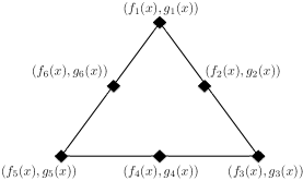
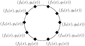
Figure 2: Oracles in the synthetic data experiments. Each has two objective functions for each two-dimensional coordinate. Top: Triangle shape finding problem. Overall, it is a multiple output function with 12 objective functions. Bottom: Sphere shape finding problem. Overall, it is a multiple output function with 20 objective functions.

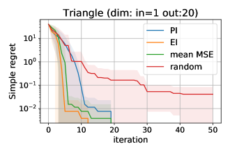
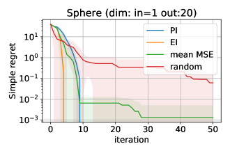
Figure 3: Comparison results of log-scale simple regret of four methods. The solid line and the shaded area represent the mean and standard deviation of 10 trials, respectively. Top: the result of the Triangle-shape finding problem. Bottom: the result of the Sphere-shape finding problem. Both experiments show that the proposed method can achieve the desired output most efficiently.

This section shows two demonstrations of the proposed method using synthetic shape finding problems.

Triangle shape finding problem

We firstly consider the problem of finding an input that achieves the desired triangle in two dimensional space. The synthetic data are created as follows: We prepared oracle functions for each $x$-axis and $y$-axis of $6$ points corresponding to each vertex and midpoint between vertexes of the triangle (see top of Figure 2). Then, 100 points as pooled dataset were sampled from the oracle functions, and 2 points from them were used as initial dataset. Here, each data point corresponds to a $12$-dimensional vector of $f_{i}(x)$ and $g_{i}(x)$, $i=1,2,...,6$. The details are described in Appendix B.1. In the experiment, we compared four methods: random sampling (random), search using only mean of the Gaussian process (mean MSE) and the proposed methods (PI and EI).

The results are shown in Figure 1 and the top of Figure 3. Figure 1 shows a process from step 1 (Top left) to step 8 (Bottom right). We can see how the model prediction (blue triangle with error bar) and the actual observation (green triangle) gradually approach the desired output (red triangle). Finally the algorithm found the desired output in seventh round. Figure 3 shows the comparison of the simple regret among the four methods. The results show the log-scale mean and standard deviation over 10 trials for each method. Obviously the proposed EI outperforms the other methods and the proposed PI is comparable to the mean MSE. Further results are shown in Appendix B.2.

Shpere shape finding problem

Second, we consider the problem of finding an input that achieves the desired sphere in two dimensional space. As in the case of the triangle, we prepared oracle functions corresponding to $x$ and $y$-axis of 10 points at equal intervals on the sphere (see bottom of Figure 2). Hence we observe the $20$-dimensional vector of $f_{i}(x)$ and $g_{i}(x)$, $i=1,2,...,10$ as data. The details are described in Appendix B.1. The other settings are the same as for the triangle.

The results are shown in the bottom of Figure 3 and Figure 7. As is the case with triangle, Figure 3 shows that the proposed method requires smaller number of iteration to reduce regrets compared to other methods. Figure 7 shows a search process from step 1 (Top left) to step 5 (Bottom right). The first and third rows are the similar plots as the Figure 1. In the second and fourth rows, the top plot shows the model behavior and the bottom plot shows the EI acquisition function. In this case, we can see that the desired output is found in the fifth observation.

4.2 Real Data Analysis

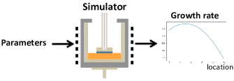
Figure 4: SiC crystal growth modeling data. Since the simulator is a black box, we can only observe the pairs of input parameters and structured-outputs.

In this section, we apply the proposed method to the crystal growth modeling data of Silicon Carbide (SiC) (Kusunoki et al., 2014; Tsunooka et al., 2018). This dataset consists of the input-output pairs. The input is parameter candidates that will be input to the SiC crystal growth model simulator, and the output is the crystal growth rate that is returned from the simulator. We have nine kinds of input parameter candidates that control the behavior of experimental equipment: thermal conductivity of felt, graphite and insulator, electrical conductivity of graphite and insulator, emissivity of solution, heat capacity of solution, reaction rate constant at crystal-solution interface, reaction rate constant at graphite-solution interface. In this experiment, we focus on the reaction rate constant at graphite-solution interface and consider this one-dimensional input. This is because empirically, the output largely vary due to the fluctuation of reaction rate constant at graphite-solution interface, that it is difficult to determine this parameter compared to other parameters. In addition, since the output, crystal growth rate, is measured at 20 locations, it is a multidimensional output observed as a 20-dimensional vector. Furthermore, since the growth rates at a near locations are expected to take a close value, this data can be regarded as a structured-output in which each dimension of the output vector has a correlation. Figure 4 shows the data generation mechanism. Our goal is to quickly find the parameters of the simulator that outputs the desired growth rate vector.

Results

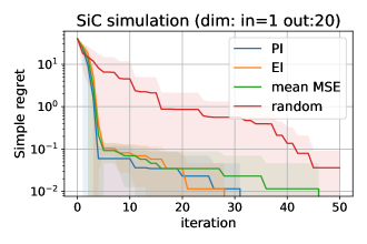
Figure 5: Comparison results of log-scale simple regret of four methods. The solid line and the shaded area represent the mean and standard deviation of 10 trials, respectively. We can see that the proposed method can achieve the desired output most efficiently.

The results are shown in Figures 5 and 6. Figure 5 shows a comparison of log-scale simple regret of the four methods. We can see that the proposed methods reduce the simple regret with fewer observations than other methods. Figure 6 shows a search process. The search proceeds from the top to the bottom. In this case, the desired growth rate vector can be found by the fourth observation. These experimental results imply that the proposed method can work effectively in the real structured-output search problems.

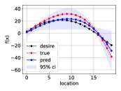
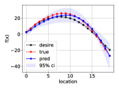
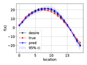
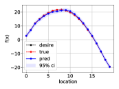
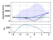
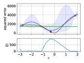
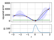
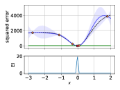
Figure 6: Shape-finding procedure and the model behavior of the proposed method using the EI acquisition function for the SiC data. Top row shows the search process in the shape space and bottom row shows the model fitting processes.

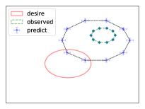
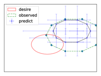
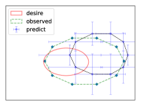
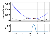
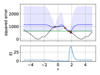
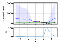
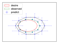
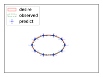
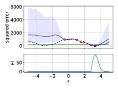
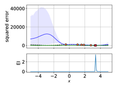
Figure 7: Results of the Sphere shape finding problem. The first and third rows show the search process in the shape space, and the second and fourth rows show the models of the objective function of active learning and the EI acquisition function in the same search process. In the shape plots, the colors red , blue and green represent the desired, predict and observed triangle respectively. In the model plots, blue line, blue shade, black line and green line represent the predictive mean, predictive variance, true squared error value and the current best squared value respectively. Furthermore, in the model plot, the sphere points represent observed points, and square points represent the next observation point specified by EI. The search process proceeds from the top left to the bottom right, and the desired sphere was found in the fifth step.

5 Concluding Remarks

We proposed a novel approach for inverse problem with structured-output. As a search strategy, two improvement-based acquisition functions, the probability of improvement and the expected improvement are derived for the problem where the output structure is expressed by the correlation between objective functions. The effectiveness of the proposed method was demonstrated by experiments with artificial shape data and real material data.

Appendix A Implementation Details

In the numerical experiments, we employ the Gaussian kernel as the covariance function $k$ of inputs which has two hyperparameters, variance and length-scale. In addition, We construct the correlation matrix ${\bm{B}}$ of the objective function as

$${\bm{B}}={\bm{L}}{\bm{L}}^{\top}+\kappa{\bm{I}}$$

where ${\bm{L}}$ and $\kappa$ are hyperparameters. All hyperparameters are estimated via marginal likelihood maximization in each iteration. We used Python 3.7.4 and the GPy package was used for Gaussian process modeling.

Appendix B Details of Synthetic Data Experiments

B.1 The Oracle Functions

The oracle functions in the synthetic experiments are as follows:

Triangle Data

For the triangle shape finding problem, we prepare the 12 oracle functions. 6 correspond to the vertices of the triangle which are given as

$$f_{1}(x) =5\sin(x),~{}g_{1}(x)=5\cos(x),$$

$$f_{2}(x) =5\sin(x)-\sqrt{|x|},~{}g_{2}(x)=5\cos(x)-2\sqrt{|x|}$$

$$f_{3}(x) =5\sin(x)+\sqrt{|x|},~{}g_{3}(x)=g_{2}(x).$$

The other 6 correspond to the midpoint of each edge of the triangle and are given by

$$f_{4}(x) =5\sin(x)-\frac{1}{2}\sqrt{|x|},~{}g_{4}(x)=5\cos(x)-\sqrt{|x|}$$

$$f_{5}(x) =5\sin(x)+\frac{1}{2}\sqrt{|x|},~{}g_{5}(x)=g_{4}(x)$$

$$f_{6}(x) =f_{1}(x),~{}g_{6}(x)=5\cos(x)-2\sqrt{|x|}.$$

Sphere Data

For the sphere shape finding problem, we prepare the 20 oracle functions correspond to the points on the one dimensional sphere. For each $m=1,...,M$ the oracle function is defined as

$$f_{m}(x)=(c(x))_{0}+r(x)\cos\left(\frac{2m\pi}{M}\right),~{}g_{m}(x)=(c(x))_{1}+r(x)\sin\left(\frac{2m\pi}{M}\right),$$

where $c(x)$ and $r(x)$ correspond to the center and the radius of the sphere respectively that are given by

$$c(x)=\left(\begin{array}[]{c}5\sin(x)\\ 5\cos(x)\end{array}\right),~{}r(x)=5|\sin(x)-\cos(x)|.$$

B.2 Experimental Results of Triangle Shape Finding Problem

In Figure 8, We show the experimental results of triangle shape finding problem as in Figure 7. As explained in Section 4, the desired triangle can be found efficiently by the proposed method.

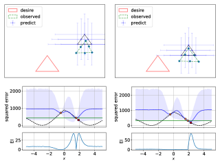
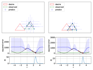
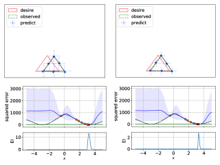
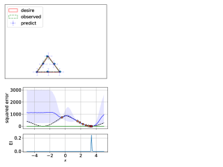
Figure 8: Results of the triangle shape finding problem. First and third rows show the search process in the shape space, and Second and fourth rows show the models of the objective function of active learning and the EI acquisition function in the same search process. In the shape plots, the colors red , blue and green represent the desired, predict and observed triangle respectively. In the model plots, blue line, blue shade, black line and green line represent the predictive mean, predictive variance, true squared error value and the current best squared value respectively. Furthermore, in the model plot, the circle points represent observed points, and square points represent the next observation point specified by EI. The search process proceeds from the top left to the bottom right, and the desired triangle was found in the seventh step.

References

- Adachi et al. (2005) S. Adachi, Y. Ogata, N. Koshikawa, S. Matsumoto, K. Kinoshita, I. Yoshizaki, T. Tsuru, H. Miyata, M. Takayanagi, and S. Yoda. Homogeneous sige crystals grown by using the traveling liquidus-zone method. journal of Crystal Growth, 280(3-4):372–377, 2005.
- Alvarez et al. (2012) M. A. Alvarez, L. Rosasco, N. D. Lawrence, et al. Kernels for vector-valued functions: A review. Foundations and Trends® in Machine Learning, 4(3):195–266, 2012.
- Ardizzone et al. (2018) L. Ardizzone, J. Kruse, S. Wirkert, D. Rahner, E. W. Pellegrini, R. S. Klessen, L. Maier-Hein, C. Rother, and U. Köthe. Analyzing inverse problems with invertible neural networks. arXiv preprint arXiv:1808.04730, 2018.
- Bannister (2017) R. Bannister. A review of operational methods of variational and ensemble-variational data assimilation. Quarterly Journal of the Royal Meteorological Society, 143(703):607–633, 2017.
- Bickel (1974) P. Bickel. Edgeworth expansions in nonparametric statistics. The Annals of Statistics, pages 1–20, 1974.
- Bonilla et al. (2008) E. V. Bonilla, K. M. Chai, and C. Williams. Multi-task gaussian process prediction. In Advances in neural information processing systems, pages 153–160, 2008.
- Brochu et al. (2010) E. Brochu, V. M. Cora, and N. De Freitas. A tutorial on bayesian optimization of expensive cost functions, with application to active user modeling and hierarchical reinforcement learning. arXiv preprint arXiv:1012.2599, 2010.
- Chen and Hobson (2019) X. Chen and M. Hobson. Bayesian surrogate learning in dynamic simulator-based regression problems. arXiv preprint arXiv:1901.08898, 2019.
- Conti and O’Hagan (2010) S. Conti and A. O’Hagan. Bayesian emulation of complex multi-output and dynamic computer models. Journal of statistical planning and inference, 140(3):640–651, 2010.
- Conti et al. (2009) S. Conti, J. P. Gosling, J. E. Oakley, and A. O’Hagan. Gaussian process emulation of dynamic computer codes. Biometrika, 96(3):663–676, 2009.
- Daggupati et al. (2010) V. Daggupati, G. Naterer, K. Gabriel, R. Gravelsins, and Z. Wang. Solid particle decomposition and hydrolysis reaction kinetics in cu–cl thermochemical hydrogen production. International Journal of Hydrogen Energy, 35(10):4877–4882, 2010.
- Dashti and Stuart (2016) M. Dashti and A. M. Stuart. The bayesian approach to inverse problems. Handbook of Uncertainty Quantification, pages 1–118, 2016.
- Davies (1980) R. B. Davies. The distribution of a linear combination of 2 random variables. Journal of the Royal Statistical Society: Series C (Applied Statistics), 29(3):323–333, 1980.
- Graybill (1976) F. A. Graybill. Theory and application of the linear model. Number QA279. G72 1976. Duxbury press North Scituate, MA, 1976.
- Hennig and Schuler (2012) P. Hennig and C. J. Schuler. Entropy search for information-efficient global optimization. Journal of Machine Learning Research, 13(Jun):1809–1837, 2012.
- Imhof (1961) J.-P. Imhof. Computing the distribution of quadratic forms in normal variables. Biometrika, 48(3/4):419–426, 1961.
- Kalnay (2003) E. Kalnay. Atmospheric modeling, data assimilation and predictability. Cambridge university press, 2003.
- Kirsch (2011) A. Kirsch. An introduction to the mathematical theory of inverse problems, volume 120. Springer Science & Business Media, 2011.
- Kusunoki et al. (2014) K. Kusunoki, N. Okada, K. Kamei, K. Moriguchi, H. Daikoku, M. Kado, H. Sakamoto, T. Bessho, and T. Ujihara. Top-seeded solution growth of three-inch-diameter 4h-sic using convection control technique. Journal of Crystal Growth, 395:68–73, 2014.
- Pav (2017) S. E. Pav. sadists: Some Additional Distributions, 2017. URL https://github.com/shabbychef/sadists. R package version 0.2.3.
- Rasmussen and Williams (2006) C. E. Rasmussen and C. K. Williams. Gaussian process for machine learning. MIT press, 2006.
- Settles (2009) B. Settles. Active learning literature survey. Technical report, University of Wisconsin-Madison Department of Computer Sciences, 2009.
- Shahriari et al. (2015) B. Shahriari, K. Swersky, Z. Wang, R. P. Adams, and N. De Freitas. Taking the human out of the loop: A review of bayesian optimization. Proceedings of the IEEE, 104(1):148–175, 2015.
- Swersky et al. (2013) K. Swersky, J. Snoek, and R. P. Adams. Multi-task bayesian optimization. In Advances in neural information processing systems, pages 2004–2012, 2013.
- Tsunooka et al. (2018) Y. Tsunooka, N. Kokubo, G. Hatasa, S. Harada, M. Tagawa, and T. Ujihara. High-speed prediction of computational fluid dynamics simulation in crystal growth. CrystEngComm, 20(41):6546–6550, 2018.
- Uhrenholt and Jensen (2019) A. K. Uhrenholt and B. S. Jensen. Efficient bayesian optimization for target vector estimation. In The 22nd International Conference on Artificial Intelligence and Statistics, pages 2661–2670, 2019.