The rotating rigid body model based on a non-twisting frame

Abstract

This work proposes and investigates a new model of the rotating rigid body based on the non-twisting frame. Such a frame consists of three mutually orthogonal unit vectors whose rotation rate around one of the three axis remains zero at all times and thus, is represented by a nonholonomic restriction. Then, the corresponding Lagrange-D’Alembert equations are formulated by employing two descriptions, the first one relying on rotations and a splitting approach, and the second one relying on constrained directors. For vanishing external moments, we prove that the new model possesses conservation laws, i.e., the kinetic energy and two nonholonomic momenta that substantially differ from the holonomic momenta preserved by the standard rigid body model. Additionally, we propose a new specialization of a class of energy-momentum integration schemes that exactly preserves the kinetic energy and the nonholonomic momenta replicating the continuous counterpart. Finally, we present numerical results that show the excellent conservation properties as well as the accuracy for the time-discretized governing equations.

1 Introduction

The rigid body is a problem of classical mechanics that has been exhaustively studied (see, e.g., [1, 2]). Its simplicity, as well as its relation with the (nonlinear) rotation group, makes of it the ideal setting to study abstract concepts of geometric mechanics, such as Poisson structures, reduction, symmetry, stability, etc. Additionally, many of the ideas that can be analyzed in the context of the rigid body can later be exploited in the study of nonlinear structural theories, such as rods and shells (as for example in [3, 4, 5]). As a result, geometrical integrators for the rigid body [6, 7] are at the root of more complex numerical integration schemes for models that involve, in one way or another, rotations [8, 9, 10, 11, 12, 13].

More specifically, the role of the rotation group is key because it is usually chosen to be the configuration space of the rigid body, when the latter has a fixed point. The rich Lie group structure of this set is responsible for much of the geometric theory of the rigid body, but it is not the only possible way to describe it. For example, the configuration of the a rigid body with a fixed point can also be described with three mutually orthogonal unit vectors. While this alternative description makes use of constraints, it has proven useful in the past for the construction of conserving numerical methods for rigid bodies, rods, and multibody systems [14, 15, 16].

In this article we explore a third route that can be followed to describe the kinematics of rigid bodies. This avenue is based on introducing a non-twisting or Bishop frame of motion [17]. This frame consists of three mutually orthogonal unit vectors whose rotation rate around one of the three axis remains zero at all times. Such a frame has proven useful to study the configuration of nonlinear Kirchhoff rods [18, 19, 20, 21], but has not received enough attention in the context of the rigid body.

Formulating the equations of motion for the rigid body in the non-twisting frame demands a construction that is different from the standard one. In particular, the definition of Bishop’s frame requires a constraint that is nonholonomic and does not admit a variational statement. Additionally, conservation laws take in this setting a different form when compared with the usual ones and whose identification is not straightforward, and the governing equations, i.e., the Lagrange-D’Alembert equations, are elegantly formulated by means of an splitting approach in terms of the covariant derivative on the unit sphere. Some of the conservation laws that take place under consideration of the non-twisitng frame may substantially differ from other nonholonomic cases that were investigated in the literature, e.g., [22, 23]. In a pure holonomic context, some attempts to reformulate the dynamics on the unit sphere by means of advanced concepts from the differential geometry are to be found in [24, 25]. However, the anisotropy of the inertial properties has been completely disregarded.

The rigid body equations with a nonholonomic constraint can be integrated in time with a conserving scheme that preserves energy and the newly identified momenta, the so-called nonholonomic momenta. This method, based on the idea of the average vector field [26, 27] preserves remarkably these invariants of the motion, exactly, resulting in accurate pictures of the rigid body dynamics. The specialization of approaches based on more elaborated conservative/dissipative integration schemes like [28] is possible as well in this context, but falls outside the scope of the current work and therefore, not addressed here.

The rest of the article has the following structure. In Section 2, the fundamental concepts from the differential geometry are presented and discussed. Section 3 presents two derivations of the equations of motion for the standard rotating rigid body. The first set of equations is a split version of the well-known Euler equations that are presented within a novel geometrical framework that relies on covariant derivatives. The second one, then, produces a totally equivalent set of equations and relies on three constrained directors. Such an approach possesses a very favorable mathematical setting that will be exploited later on to derive an structure-preserving integration algorithm. In Section 4, the non-twisting condition is enforced for both fully equivalent formulations. Additionally, new conservation laws are identified in the continuous setting. Section 5 starts with the energy-momentum integration scheme for the director-based formulation and then it is modified for the nonholonomic case. The conservation properties are identified analytically for the discrete setting, replicating their continuous counterparts. In Section 6, numerical results that show the excellent performance of the new energy-momentum algorithm are presented and discussed. Finally, Section 7 closes this work with a summary.

2 Relevant geometrical concepts

The governing equations of the rigid body are posed on nonlinear manifolds. We briefly summarize the essential geometrical concepts required for a complete description of the model (see, e.g., [29, 25] for more comprehensive expositions).

2.1 The unit sphere

The unit sphere $S^{2}$ is a nonlinear, compact, two-dimensional manifold that often appears in the configuration spaces of solid mechanics, be it the rigid body, rods, or shells [30, 31, 32, 33, 13]. As an embedded set on Euclidean space, it is defined as

$$S^{2}:=\left\{\bm{d}\in\mathbb{R}^{3}\mid\bm{d}\cdot\bm{d}=1\right\},$$ (1)

where the dot product is the standard one in $\mathbb{R}^{3}$. The tangent bundle of the unit 2-sphere is also a manifold defined as

$$TS^{2}:=\left\{(\bm{d},\bm{v}),\ \bm{d}\in S^{2},\ \bm{v}\in\mathbb{R}^{3},\ \bm{d}\cdot\bm{v}=0\right\}.$$ (2)

Alternatively, tangent vectors of $S^{2}$ to a point $\bm{d}$ are those defined by the expressions:

$$\bm{v}=\bm{w}\times\bm{d}\,,\quad\mathrm{with}\quad\bm{w}\cdot\bm{d}=0\ ,$$ (3)

where the product “$\times$” is the standard cross product in $\mathbb{R}^{3}$.

In contrast with the space of rotations, to be studied in more detail later, the unit sphere does not have a group structure, but instead it has that of a Riemannian manifold. The connection of this set can be more easily explained by considering it to be an embedded manifold in $\mathbb{R}^{3}$. As such, the covariant derivative of a smooth vector field $\bm{v}:S^{2}\to TS^{2}$ along a vector field $\bm{w}:S^{2}\to TS^{2}$ is the vector field $\nabla_{\bm{w}}\bm{v}\in TS^{2}$ that evaluated at $\bm{d}$ is precisely the projection of the derivative $D\bm{v}$ in the direction of $\bm{w}$ onto the tangent plane to $\bm{d}$. Hence, denoting as $\bm{I}$ the unit second order tensor and $\otimes$ the outer product between vectors, both on $\mathbb{R}^{3}$, this projection can be simply written as

$$\nabla_{\bm{w}}\bm{v}:=(\bm{I}-\bm{d}\otimes\bm{d})\;D\bm{v}\cdot\bm{w}\ .$$ (4)

When $\bm{d}:(a,b)\to S^{2}$ is a smooth one-parameter curve on the unit sphere and $\bm{d}^{\prime}$ its derivative, the covariant derivative of a smooth vector field $\bm{v}:S^{2}\to TS^{2}$ in the direction of $\bm{d}^{\prime}$ has an expression that follows from Eq. (4), that is,

$$\nabla_{\bm{d}^{\prime}}\bm{v}=(\bm{I}-\bm{d}\otimes\bm{d})\;D\bm{v}\cdot\bm{d}^{\prime}=(\bm{v}\circ\bm{d})^{\prime}-\left((\bm{v}\circ\bm{d})^{\prime}\cdot\bm{d}\right)\bm{d},$$ (5)

which, as before, is nothing but the projection of $(\bm{v}\circ\bm{d})^{\prime}$ onto the tangent space $T_{\bm{d}}S^{2}$, and the symbol “$\circ$” stands for composition. The covariant derivative allows to compare two tangent vectors belonging to different tangent spaces. By means of the parallel transport, one vector can be transported from its tangent space to the space of the other one. Then, all the desired comparisons can be made over objects belonging to the same space.

The exponential map $\exp:T_{\bm{d}_{0}}S^{2}\to S^{2}$ is a surjective application with a closed form expression given by the formula

$$\exp_{\bm{d}_{0}}(\bm{v}_{0})=\cos(|\bm{v}_{0}|)\bm{d}_{0}+\sin(|\bm{v}_{0}|)\frac{\bm{v}_{0}}{|\bm{v}_{0}|}\,,$$ (6)

where $\bm{v}_{0}$ must be a tangent vector on $T_{\bm{d}_{0}}S^{2}$ and $|\cdot|$ denotes the Euclidean vector norm. The inverse of the exponential function is the logarithmic map $\log:S^{2}\to T_{\bm{d}_{0}}S^{2}$, for which also there is a closed form expression that reads

$$\log_{\bm{d}_{0}}(\bm{d})=\arccos(\bm{d}_{0}\cdot\bm{d})\frac{(\bm{I}-\bm{d}_{0}\otimes\bm{d}_{0})\bm{d}}{|(\bm{I}-\bm{d}_{0}\otimes\bm{d}_{0})\bm{d}|},$$ (7)

with $\bm{d}_{0}\neq-\bm{d}$. The geodesic $\bm{d}_{\mathrm{G}}(s)$ for $s\in[0,1]$ with $\bm{d}_{\mathrm{G}}(0)=\bm{d}_{0}$ and $\bm{d}^{\prime}_{\mathrm{G}}(0)=\bm{v}_{0}$ is a great arch on the sphere obtained as the solution of the equation

$$\nabla_{\bm{d}^{\prime}}{\bm{d}^{\prime}}=\bm{0}\,,$$ (8)

with the explicit form

$$\bm{d}_{\mathrm{G}}(s)=\cos(|\bm{v}_{0}|s)\bm{d}_{0}+\sin(|\bm{v}_{0}|s)\frac{\bm{v}_{0}}{|\bm{v}_{0}|}\,.$$ (9)

The parallel transport of $\bm{w}_{0}\in T_{\bm{d}_{0}}S^{2}\mapsto\bm{w}\in T_{\bm{d}}S^{2}$ along the geodesic $\bm{d}_{\mathrm{G}}$ is then given by

$$\bm{w}=\left(\bm{I}-\frac{1}{\arccos^{2}(\bm{d}_{0}\cdot\bm{d}_{\mathrm{G}})}\left(\log_{\bm{d}_{0}}\bm{d}_{\mathrm{G}}+\log_{\bm{d}_{\mathrm{G}}}\bm{d}_{0}\right)\otimes\log_{\bm{d}_{0}}\bm{d}_{\mathrm{G}}\right)\bm{w}_{0}\,,$$ (10)

and verifies

$$\nabla_{\bm{w}}{\bm{d}^{\prime}}=(\bm{I}-\bm{d}\otimes\bm{d})\bm{w}^{\prime}=\bm{0}\,.$$ (11)

More details about the expressions (6) to (10) can be found in [34, 35].

Given the definitions (1) and (2) of the unit sphere and its tangent bundle, we recognize that there exists an isomorphism

$$\mathbb{R}^{3}\cong T_{\bm{d}}S^{2}\oplus\mathrm{span}(\bm{d}),$$ (12)

for any $\bm{d}\in S^{2}$. Given now two directors $\bm{d},\tilde{\bm{d}}$, we say that a second order tensor $\bm{T}:\mathbb{R}^{3}\to\mathbb{R}^{3}$ splits from $\bm{d}$ to $\tilde{\bm{d}}$ if it can be written in the form

$$\bm{T}={\bm{T}}_{\perp}+{\bm{T}}_{\parallel}\>,$$ (13)

where ${\bm{T}}_{\perp}$ is a bijection from $T_{\bm{d}}S^{2}$ to $T_{\tilde{\bm{d}}}S^{2}$ with $\ker({\bm{T}}_{\perp})=\hbox{span}(\bm{d})$, and ${\bm{T}}_{\parallel}$ is a bijection from $\hbox{span}(\bm{d})$ to $\hbox{span}(\tilde{\bm{d}})$ with $\ker({\bm{T}}_{\parallel})\equiv T_{\bm{d}}S^{2}$. The split (13) depends on the pair $\bm{d},\tilde{\bm{d}}$ but it is not indicated explicitly in order to simplify the notation.

2.2 The special orthogonal group

Classical descriptions of rigid body kinematics are invariably based on the definition of their configuration space as the set of proper orthogonal second order tensors, that is, the special orthogonal group, defined as

$$SO(3):=\left\{\bm{\mathit{\Lambda}}\in\mathbb{R}^{3\times 3},\ \bm{\mathit{\Lambda}}^{T}\bm{\mathit{\Lambda}}=\bm{I},\ \det{\bm{\mathit{\Lambda}}}=+1\right\}.$$ (14)

This smooth manifold has a group-like structure when considered with the tensor multiplication operation, thus it is a Lie group. Its associated Lie algebra is the linear set

$$so(3):=\left\{\hat{\bm{w}}\in\mathbb{R}^{3\times 3},\ \hat{\bm{w}}=-\hat{\bm{w}}^{T}\right\}.$$ (15)

Later, it will be convenient to exploit the isomorphism that exists between three-dimensional real vectors and $so(3)$. To see this, consider the map $\hat{(\cdot)}:\mathbb{R}^{3}\to so(3)$ such that for all $\bm{w},\bm{a}\in\mathbb{R}^{3}$, the tensor $\hat{\bm{w}}\in so(3)$ satisfies $\hat{\bm{w}}\bm{a}=\bm{w}\times\bm{a}$. Here, $\bm{w}$ is referred to as the axial vector of $\hat{\bm{w}}$, which is a skew-symmetric tensor, and we also write $\mathrm{skew}[\bm{w}]=\hat{\bm{w}}$. Being a Lie group, the space of rotations has an exponential map $\exp:so(3)\to SO(3)$ whose closed form expression is Rodrigues’ formula

$$\exp[\hat{\bm{\theta}}]:=\bm{I}+\frac{\sin\theta}{\theta}\hat{\bm{\theta}}+\frac{1}{2}\frac{\sin^{2}(\theta/2)}{(\theta/2)^{2}}\hat{\bm{\theta}}^{2}\ ,$$ (16)

with $\bm{\theta}\in\mathbb{R}^{3}$, $\theta=|\bm{\theta}|$. The linearization of the exponential map is simplified by introducing the map $\mathrm{dexp}:so(3)\to\mathbb{R}^{3\times 3}$ that satisfies

$$\frac{\mathrm{d}}{\mathrm{d}\epsilon}\exp[\hat{\bm{\theta}}(\epsilon)]=\mathrm{skew}\left[\mathrm{dexp}[\hat{\bm{\theta}}(\epsilon)]\frac{\mathrm{d}}{\mathrm{d}\epsilon}\bm{\theta}(\epsilon)\right]\exp[\hat{\bm{\theta}}(\epsilon)]$$ (17)

for every $\bm{\theta}:\mathbb{R}\to\mathbb{R}^{3}$. A closed-form expression for this map, as well as more details regarding the numerical treatment of rotations can be found elsewhere [36, 7, 13].

2.3 The notion of twist and the non-twisting frame

Let $\bm{d}_{3}:\left[0,T\right]\rightarrow S^{2}$ indicate a curve of directors parameterized by time $t\in[0,T]$. Now, let us consider two other curves $\bm{d}_{1},\bm{d}_{2}:[0,T]\to S^{2}$ such that $\{\bm{d}_{1}(t),\bm{d}_{2}(t),\bm{d}_{3}(t)\}$ are mutually orthogonal for all $t\in[0,T]$. We say that the triad $\{\bm{d}_{1},\bm{d}_{2},\bm{d}_{3}\}$ moves without twist if

$$\dot{\bm{d}}_{1}\cdot\bm{d}_{2}=\dot{\bm{d}}_{2}\cdot\bm{d}_{1}=0\ ,$$ (18)

where the overdot refers to the derivative with respect to time. Given the initial value of the triad $\{\bm{d}_{1}(0),\bm{d}_{2}(0),\bm{d}_{3}(0)\}=\{\bm{D}_{1},\bm{D}_{2},\bm{D}_{3}\}$, there is a map $\bm{\chi}:[0,T]\to SO(3)$ transforming it to the frame $\{\bm{d}_{1},\bm{d}_{2},\bm{d}_{3}\}$ that evolves without twist, and whose closed form is

$$\bm{\chi}=\bm{d}_{1}\otimes\bm{D}_{1}+\bm{d}_{2}\otimes\bm{D}_{2}+\bm{d}_{3}\otimes\bm{D}_{3}\,.$$ (19)

The non-twisting frame has Darboux vector

$$\bm{w}_{\bm{\chi}}=\bm{d}_{3}\times\dot{\bm{d}}_{3}\>,$$ (20)

and it is related to parallel transport in the sphere. To see this relation, consider again the same non-twisting frame as before. Then, we recall that a vector field $\bm{v}\in T_{\bm{d}_{3}}S^{2}$ is said to be parallel-transported along $\bm{d}_{3}$ if and only if $\nabla_{\bm{v}}{\dot{\bm{d}}_{3}}=\bm{0}$. An consequence of this is that

$$\dot{\bm{d}}_{3}\cdot\dot{\bm{d}}_{1}=\dot{\bm{d}}_{3}\cdot(\bm{w}_{\bm{\chi}}\times\bm{d}_{1})=0,$$ (21)

and similarly

$$\dot{\bm{d}}_{3}\cdot\dot{\bm{d}}_{2}=\dot{\bm{d}}_{3}\cdot(\bm{w}_{\bm{\chi}}\times\bm{d}_{2})=0\,.$$ (22)

In addition, we have that

$$\begin{split}\dot{\bm{d}}_{1}\cdot\dot{\bm{d}}_{2}=(\bm{w}_{\bm{\chi}}\times\bm{d}_{1})\cdot(\bm{w}_{\bm{\chi}}\times\bm{d}_{2})=(\bm{d}_{1}\cdot\dot{\bm{d}}_{3})(\bm{d}_{2}\cdot\dot{\bm{d}}_{3})\,,\end{split}$$ (23)

which is merely the product of the angular velocity components and can be interpreted as a scalar curvature.

To define precisely the concept of twist, let us consider the rotation $\exp[\psi\>\hat{\bm{d}}_{3}]$, with $\psi:[0,T]\to S^{1}$ (the unit 1-sphere), and the rotated triad $\{\bm{d}_{1}^{\psi},\bm{d}_{2}^{\psi},\bm{d}_{3}\}=\exp[\psi\>\hat{\bm{d}}_{3}]\{\bm{d}_{1},\bm{d}_{2},\bm{d}_{3}\}$. Then,

$$\bm{d}_{1}^{\psi}=\cos(\psi)\bm{d}_{1}+\sin(\psi)\bm{d}_{2}\qquad\mathrm{and}\qquad\bm{d}_{2}^{\psi}=-\sin(\psi)\bm{d}_{1}+\cos(\psi)\bm{d}_{1},$$ (24)

and the Darboux vector of the rotated triad is

$$\bm{w}_{\exp[\psi\>\hat{\bm{d}}_{3}]\bm{\chi}}=\bm{d}_{3}\times\dot{\bm{d}}_{3}+\dot{\psi}\bm{d}_{3},$$ (25)

or, equivalently,

$$\bm{w}_{\exp[\psi\>\hat{\bm{d}}_{3}]\bm{\chi}}=-(\bm{d}_{2}^{\psi}\cdot\dot{\bm{d}}_{3})\bm{d}_{1}^{\psi}+(\bm{d}_{1}^{\psi}\cdot\dot{\bm{d}}_{3})\bm{d}_{2}^{\psi}+\dot{\psi}\bm{d}_{3}\,.$$ (26)

In this last expression, we identify the twist rate $\dot{\psi}$ and the twist angle $\psi$, respectively, as the rotation velocity component on the $\bm{d}_{3}$ direction and the rotation angle about this same vector (for further details, see [17, 37]). The previous calculations show that the frame $\{\bm{d}_{1},\bm{d}_{2},\bm{d}_{3}\}$ — known as the natural or Bishop frame in the context of one-parameter curves embedded in the ambient space — is the unique one obtained by transporting $\{\bm{D}_{1},\bm{D}_{2},\bm{D}_{3}\}$ without twist. In this context, a summary of recent advances and open problems are presented for instance in [38].

3 Standard rotating rigid body

In this section, we review the classical rotating rigid body model, which we take as the starting point for our developments. We present this model, however, in an unusual fashion. In it, the governing equations of the body appear in split form. This refers to the fact that, for a given director $\bm{d}_{3}$, the dynamics of the body that takes place in the cotangent space $T^{*}_{\bm{d}_{3}}S^{2}$ is separated from that one corresponding to the reciprocal normal space $N^{*}_{\bm{d}_{3}}S^{2}\equiv\textrm{span}(\bm{d}_{3})$. In order to do this, we have employed the identifications

$$\mathbb{R}^{3}\cong T_{\bm{d}_{3}}S^{2}\oplus\textrm{span}(\bm{d}_{3})\cong T^{*}_{\bm{d}_{3}}S^{2}\oplus\textrm{span}(\bm{d}_{3})\,.$$ (27)

3.1 Kinematic description

As customary, a rotating rigid body is defined to be a three-dimensional non-deformable body. The state of such a body, when one of its points is fixed, can be described by a rotating frame whose orientation is given by a rotation tensor. Thus, the configuration manifold is $Q\equiv SO(3)$.

Let us now study the motion of a rotating rigid body, that is, a time-parameterized curve in configuration space $\bm{\mathit{\Lambda}}:[0,T]\to Q$. The generalized velocity of the rotating rigid body belongs, for every $t\in[0,T]$, to the tangent bundle

$$TQ:=\left\{(\bm{\mathit{\Lambda}},\dot{\bm{\mathit{\Lambda}}}),\bm{\mathit{\Lambda}}\in SO(3),\bm{\mathit{\Lambda}}^{T}\dot{\bm{\mathit{\Lambda}}}\in so(3)\right\}.$$ (28)

The time derivative of the rotation tensor can be written as

$$\dot{\bm{\mathit{\Lambda}}}=\hat{\bm{w}}\bm{\mathit{\Lambda}}=\bm{\mathit{\Lambda}}\widehat{\bm{W}}\ ,$$ (29)

where $\bm{w}$ and $\bm{W}$ are the spatial and convected angular velocities, respectively.

Let $\{\bm{E}_{1},\bm{E}_{2},\bm{E}_{3}\}$ be a fixed basis of the ambient space. Then, if $\bm{d}_{i}=\bm{\mathit{\Lambda}}\bm{E}_{i}$, with $i=1,2,3$ we can use Eq. (27) to split the rotation vectors as in

$$\bm{w}=\bm{w}_{\perp}+w_{\parallel}\bm{d}_{3}\ ,\qquad\bm{W}=\bm{W}_{\perp}+W_{\parallel}\bm{d}_{3}\ .$$ (30)

Then, using the relations (29), we identify

$$\bm{w}_{\perp}=\bm{d}_{3}\times\dot{\bm{d}_{3}}\ ,\qquad\bm{W}_{\perp}=\bm{\mathit{\Lambda}}^{T}\bm{w}_{\perp}\ .\qquad$$ (31)

3.2 Kinetic energy and angular momentum

Let us now select a fixed Cartesian basis of $\mathbb{R}^{3}$ denoted as $\{\bm{D}_{i}\}_{i=1}^{3}$, where the third vector coincides with one of the principal directions of the convected inertia tensor $\bm{J}:\mathbb{R}^{3}\to\mathbb{R}^{3}$ of the body, a symmetric, second order, positive definite tensor. Thus, this tensor splits from $\bm{D}_{3}$ to $\bm{D}_{3}$ and we write

$$\bm{J}=\bm{J}_{\perp}+J_{\parallel}\,\bm{D}_{3}\otimes\bm{D}_{3}\ ,$$ (32)

where $\bm{J}_{\perp}$ maps bijectively $\mathrm{span}(\bm{D}_{1},\bm{D}_{2})$ onto itself and satisfies $\bm{J}_{\perp}\bm{D}_{3}=\bm{0}$.

The kinetic energy of a rigid body with a fixed point is defined as the quadratic form

$$K:=\frac{1}{2}\bm{W}\cdot\bm{J}\bm{W}=\frac{1}{2}\bm{w}\cdot\bm{j}\bm{w}\ ,$$ (33)

where $\bm{j}$ is the spatial inertia tensor, the push-forward of the convected inertia, and defined as

$$\bm{j}:=\bm{\mathit{\Lambda}}\bm{J}\bm{\mathit{\Lambda}}^{T}\ .$$ (34)

Let $\bm{d}_{3}=\bm{\mathit{\Lambda}}\bm{D}_{3}$. Given the relationship between the convected and spatial inertia, it follows that the latter also splits, this time from $\bm{d}_{3}$ to $\bm{d}_{3}$, and thus

$$\bm{j}=\bm{j}_{\perp}+j_{\parallel}\,\bm{d}_{3}\otimes\bm{d}_{3}\ ,$$ (35)

where now $\bm{j}_{\perp}$ maps bijectively $\mathrm{span}(\bm{d}_{1},\bm{d}_{2})$ onto itself and satisfies $\bm{j}_{\perp}\bm{d}_{3}=\bm{0}$.

As a consequence of the structure of the inertia tensor, the kinetic energy of a rotating rigid body can be written in either of the following equivalent ways:

$$\frac{1}{2}\bm{w}\cdot\bm{j}\bm{w}=\frac{1}{2}\bm{W}\cdot\bm{J}\bm{W}=\frac{1}{2}\bm{W}_{\perp}\cdot\bm{J}_{\perp}\bm{W}_{\perp}+\frac{1}{2}J_{\parallel}\,W_{\parallel}^{2}=\frac{1}{2}\bm{w}_{\perp}\cdot\bm{j}_{\perp}\bm{w}_{\perp}+\frac{1}{2}j_{\parallel}\,w_{\parallel}^{2}.$$ (36)

The angular momentum of the rotating rigid body is conjugate to the angular velocity as in

$$\qquad\bm{\pi}:=\frac{\partial K}{\partial\bm{w}}=\bm{j}\bm{w}\>,$$ (37)

and we note that we can introduce a convected version of the momentum $\bm{\pi}$ by pulling it back with the rotating tensor and defining

$$\bm{\mathit{\Pi}}:=\bm{\mathit{\Lambda}}^{T}\bm{\pi}=\frac{\partial K}{\partial\bm{W}}\ .$$ (38)

Due to the particular structure of the inertia, the momentum can also be split, as before, as in

$$\bm{\pi}=\bm{\pi}_{\perp}+\pi_{\parallel}\bm{d}_{3}\ ,\qquad\bm{\mathit{\Pi}}=\bm{\mathit{\Pi}}_{\perp}+\mathit{\Pi}_{\parallel}\bm{d}_{3},$$ (39)

with

$$\bm{\pi}_{\perp}=\bm{j}_{\perp}\bm{w}_{\perp}\ ,\qquad\bm{\mathit{\Pi}}_{\perp}=\bm{J}_{\perp}\bm{W}_{\perp},\qquad\pi_{\parallel}=\mathit{\Pi}_{\parallel}=j_{\parallel}w_{\parallel}=J_{\parallel}W_{\parallel}\ .$$ (40)

3.3 Variations of the motion rates

The governing equations of the rigid body will be obtained using Hamilton’s principle of stationary action, using calculus of variations. We gather next some results that will prove necessary for the computation of the functional derivatives and, later, for the linearization of the model.

To introduce these concepts, let us consider a curve of configurations $\bm{\mathit{\Lambda}}_{\iota}(t)$ parametrized by the scalar $\iota$ and given by

$$\bm{\mathit{\Lambda}}_{\iota}(t)=\exp[\iota\,\widehat{\delta\bm{\theta}}(t)]\bm{\mathit{\Lambda}}(t)\,,$$ (41)

where $\delta\bm{\theta}:[0,T]\to\mathbb{R}^{3}$ represents all arbitrary variations that satisfy

$$\delta\bm{\theta}(0)=\delta\bm{\theta}(T)=\bm{0}\ .$$ (42)

The curve $\bm{\mathit{\Lambda}}_{\iota}$ passes through the configuration $\bm{\mathit{\Lambda}}$ when $\iota=0$ and has tangent at this point

$$\left.\frac{\partial}{\partial t}\right|_{\iota=0}\bm{\mathit{\Lambda}}_{\iota}=\widehat{\delta\bm{\theta}}\bm{\mathit{\Lambda}}\,.$$ (43)

For future reference, let us calculate the variation of the derivative $\dot{\bm{\mathit{\Lambda}}}$. To do so, let us first define the temporal derivative of the perturbed rotation, that is,

$$\begin{split}\frac{\partial}{\partial t}\bm{\mathit{\Lambda}}_{\iota}&=\frac{\partial}{\partial t}\exp[\iota\widehat{\delta\bm{\theta}}]\bm{\mathit{\Lambda}}=\mathrm{skew}\left[\mathrm{dexp}[\iota\widehat{\delta\bm{\theta}}]\iota\delta\dot{\bm{\theta}}\right]\bm{\mathit{\Lambda}}+\exp[\iota\widehat{\delta\bm{\theta}}]\dot{\bm{\mathit{\Lambda}}}\ .\end{split}$$ (44)

Then, the variation of $\dot{\bm{\mathit{\Lambda}}}$ is just

$$\delta(\dot{\bm{\mathit{\Lambda}}})=\left.\frac{\partial}{\partial\iota}\right|_{\iota=0}\frac{\partial}{\partial t}\bm{\mathit{\Lambda}}_{\iota}=\widehat{\delta\dot{\bm{\theta}}}\bm{\mathit{\Lambda}}+\widehat{\delta\bm{\theta}}\dot{\bm{\mathit{\Lambda}}}\ .$$ (45)

With the previous results at hand, we can now proceed to calculate the variations of the convected angular velocities, as summarized in the following theorem.

Theorem 3.1.

The variations of the convected angular velocities $(\bm{W}_{\perp},W_{\parallel})$ are

$$\delta\bm{W}_{\perp} ={\bm{{\mathit{\Lambda}}}}^{T}(\bm{I}-\bm{d}_{3}\otimes\bm{d}_{3})\delta\dot{\bm{\theta}}\,,$$ (46a)

$$\delta W_{\parallel} =\bm{d}_{3}\cdot\delta\dot{\bm{\theta}}\,.$$ (46b)

Proof.

The convected angular velocities of the one-parameter curve of configurations $\bm{\mathit{\Lambda}}_{\iota}$ are

$$\bm{W}_{\perp,\iota}=\bm{D}_{3}\times(\bm{\mathit{\Lambda}}^{T}_{\iota}\dot{\bm{d}}_{3,\iota})\quad\textrm{and}\quad W_{\parallel,_{\iota}}=\bm{d}_{2,\iota}\cdot\dot{\bm{d}}_{1,\iota}\,,$$ (47)

where $\bm{d}_{i,\iota}=\bm{\mathit{\Lambda}}_{\iota}\bm{D}_{i}$. The variation of the angular velocity perpendicular to $\bm{D}_{3}$ is obtained from its definition employing some algebraic manipulations and expression (45) as follows:

$$\begin{split}\delta\bm{W}_{\perp}&=\left.\frac{\partial}{\partial\iota}\right|_{\iota=0}\left(\bm{D}_{3}\times\left(\bm{\mathit{\Lambda}}^{T}_{\iota}\dot{\bm{d}}_{3,\iota}\right)\right)\\ &=\bm{D}_{3}\times\left(\delta\bm{\mathit{\Lambda}}^{T}\dot{\bm{\mathit{\Lambda}}}\bm{D}_{3}+\bm{\mathit{\Lambda}}^{T}\delta\dot{\bm{\mathit{\Lambda}}}\bm{D}_{3}\right)\\ &=\bm{\mathit{\Lambda}}^{T}\left(\bm{d}_{3}\times\left(\widehat{\delta\dot{\bm{\theta}}}\times\bm{d}_{3}\right)\right)\\ &=\bm{\mathit{\Lambda}}^{T}\left(\delta\dot{\bm{\theta}}-\left(\delta\dot{\bm{\theta}}\cdot\bm{d}_{3}\right)\bm{d}_{3}\right)\\ &=\bm{\mathit{\Lambda}}^{T}(\bm{I}-\bm{d}_{3}\otimes\bm{d}_{3})\delta\dot{\bm{\theta}}\ .\end{split}$$ (48)

The variation of the angular velocity parallel to $\bm{D}_{3}$ follows similar steps:

$$\begin{split}\delta W_{\parallel}&=\left.\frac{\partial}{\partial\iota}\right|_{\iota=0}\left(\bm{d}_{2,\iota}\cdot\dot{\bm{d}}_{1,\iota}\right)\\ &=\widehat{\delta\bm{\theta}}\bm{\mathit{\Lambda}}\bm{D}_{2}\cdot\dot{\bm{\mathit{\Lambda}}}\bm{D}_{1}+\bm{\mathit{\Lambda}}\bm{D}_{2}\cdot\left(\widehat{\delta\dot{\bm{\theta}}}\bm{\mathit{\Lambda}}+\widehat{\delta\bm{\theta}}\dot{\bm{\mathit{\Lambda}}}\right)\bm{D}_{1}\\ &=\bm{d}_{1}\times\bm{d}_{2}\cdot\delta\dot{\bm{\theta}}\\ &=\bm{d}_{3}\cdot\delta\dot{\bm{\theta}}\ .\end{split}$$ (49)

∎

3.4 Governing equations and invariants

Here, we derive the governing equations of the rotating rigid body model and the concomitant conservation laws. Hamilton’s principle of stationary action states that the governing equations are the Euler-Lagrange equations of the action functional

$$S=\int^{T}_{0}K\,\textrm{d}t\,,$$ (50)

with unknown fields $(\bm{\mathit{\Lambda}},\dot{\bm{\mathit{\Lambda}}})\in TQ$.

Theorem 3.2.

The equations of motion, i.e., the Euler-Lagrange equations, for the standard rotating rigid body model in split form are:

$$\nabla_{\dot{\bm{d}}_{3}}{\bm{\pi}_{\perp}}+\pi_{\parallel}\dot{\bm{d}}_{3} =\bm{0}\,,$$ (51a)

$$\dot{\pi}_{\parallel}+\bm{\pi}_{\perp}\cdot\dot{\bm{d}}_{3} =0\,.$$ (51b)

The pertaining initial conditions are:

$$\bm{\mathit{\Lambda}}(0)=\bar{\bm{\mathit{\Lambda}}}\,,\quad\bm{w}_{\perp}(0)=\bar{\bm{w}}_{\perp}\,,\quad w_{\parallel}(0)=\bar{w}_{\parallel}\,.$$ (52)

Proof.

The theorem follows from the systematic calculation of $\delta S$, the variation of the action, based on the variation of the convected angular velocities of Eq. (46), thus we omit a detailed derivation. Eq. (51), which is presented in its split form, is equivalent to Euler’s equations which state that the spatial angular momentum is preserved, i.e., $\dot{\bm{\pi}}=\bm{0}$. This is easily proven as follows

$$\begin{split}\bm{0}&=\dot{\bm{\pi}}\\ &=(\bm{I}-\bm{d}_{3}\otimes\bm{d}_{3})\dot{\bm{\pi}}+(\bm{d}_{3}\cdot\dot{\bm{\pi}})\bm{d}_{3}\\ &=(\bm{I}-\bm{d}_{3}\otimes\bm{d}_{3})(\dot{\bm{\pi}}_{\perp}+\dot{\pi}_{\parallel}\bm{d}_{3}+\pi_{\parallel}\dot{\bm{d}}_{3})+\bm{d}_{3}\cdot(\dot{\bm{\pi}}_{\perp}+\dot{\pi}_{\parallel}\bm{d}_{3}+\pi_{\parallel}\dot{\bm{d}}_{3})\bm{d}_{3}\\ &=\underbrace{\nabla_{\dot{\bm{d}}_{3}}{\bm{\pi}_{\perp}}+\pi_{\parallel}\dot{\bm{d}}_{3}}_{\in\>T^{*}_{\bm{d}_{3}}S^{2}}+\underbrace{(\dot{\pi}_{\parallel}+\dot{\bm{\pi}}_{\perp}\cdot\bm{d}_{3})\bm{d}_{3}}_{\in\>\mathrm{span}(\bm{d}_{3})}\,.\end{split}$$ (53)

∎

Theorem 3.3.

The conservation laws of the rotating rigid body are:

$$K =\frac{1}{2}\bm{W}\cdot\bm{J}\bm{W}=\frac{1}{2}\bm{w}\cdot\bm{j}\bm{w}=\text{const.}\,,$$ (54a)

$$\bm{\pi} =\bm{j}\bm{w}=\bm{\mathit{\Lambda}}\bm{J}\bm{W}=\text{const.}\,.$$ (54b)

Proof.

This is an standard result and thus, we omit further details. ∎

Remark.

To include external moments acting on the standard rotating rigid body it is necessary to calculate the associated virtual work as follows

$$\delta W=\delta\bm{\theta}_{\perp}\cdot\bm{m}^{\mathrm{ext}}_{\perp}+\delta\theta_{\parallel}m^{\mathrm{ext}}_{\parallel}\,,$$ (55)

and add this contribution to the variation of the action.

3.5 Model equations based on directors

Here, we present an alternative set of governing equations for the rotating rigid body model that will be used later to formulate a structure preserving algorithm. For this purpose, let us define the following configuration space

$$Q:=\{\bm{q}=(\bm{d}_{1},\bm{d}_{2},\bm{d}_{3})\in S^{2}\times S^{2}\times S^{2}\mid\bm{d}_{i}\cdot\bm{d}_{j}=0,i\neq j\}\cong SO(3)\,,$$ (56)

whose tangent space at the point $\bm{q}$ is given by

$$T_{\bm{q}}Q:=\{\dot{\bm{q}}=(\dot{\bm{d}}_{1},\dot{\bm{d}}_{2},\dot{\bm{d}}_{3})\mid\dot{\bm{d}}_{i}=\bm{\omega}\times\bm{d}_{i},\bm{\omega}\in\mathbb{R}^{3}\}\,.$$ (57)

Now, we start by defining the rigid body as the bounded set ${\cal B}_{0}\subset\mathbb{R}^{3}$ of points

$$\bm{X}=\theta^{1}\bm{D}_{1}+\theta^{2}\bm{D}_{2}+\theta^{3}\bm{D}_{3}$$ (58)

where $(\theta^{1},\theta^{2},\theta^{3})$ are the material coordinates of the point and $\{\bm{D}_{i}\}_{i=1}^{3}$ are three orthogonal directors, with the third one oriented in the direction of the principal axis of inertia and such that $\bm{D}_{3}=\bm{D}_{1}\times\bm{D}_{2}$. The position of the point $\bm{X}$ at time $t\in[0,T]$ is denoted as $\bm{x}(t)\in\mathbb{R}^{3}$ and given by

$$\bm{x}(t)=\bm{\varphi}(\theta^{1},\theta^{2},\theta^{3};t)=\theta^{1}\bm{d}_{1}(t)+\theta^{2}\bm{d}_{2}(t)+\theta^{3}\bm{d}_{3}(t)$$ (59)

with $(\bm{d}_{1},\bm{d}_{2},\bm{d}_{3})=\bm{q}\in Q$, for all $t$. On this basis, there must be a rotation tensor $\bm{\mathit{\Lambda}}(t)=\bm{d}_{i}(t)\otimes\bm{D}_{i}$, where we have employed the sum convention for repeated indices, such that $\bm{d}_{i}(t)=\bm{\mathit{\Lambda}}(t)\bm{D}_{i}$. The material velocity of the particle $\bm{X}$ is the vector $\dot{\bm{x}}(t)\in\mathbb{R}^{3}$ that can be written as

$$\dot{\bm{x}}(t)=\dot{\bm{\varphi}}(\theta^{1},\theta^{2},\theta^{3};t)=\theta^{1}\dot{\bm{d}}_{1}(t)+\theta^{2}\dot{\bm{d}}_{2}(t)+\theta^{3}\dot{\bm{d}}_{3}(t)$$ (60)

with $(\dot{\bm{d}}_{1},\dot{\bm{d}}_{2},\dot{\bm{d}}_{3})=\dot{\bm{q}}\in T_{\bm{q}}Q$ representing three director velocity vectors.

To construct the dynamic equations of the model, assume the body ${\cal B}_{0}$ has a density $\rho_{0}$ per unit of reference volume and hence its total kinetic energy, or Lagrangian, can be formulated as

$$K=\int_{{\cal B}_{0}}\frac{\rho_{0}}{2}|\dot{\bm{x}}|^{2}\,\mathrm{d}{\cal B}_{0}\ .$$ (61)

To employ Hamilton’s principle of stationary action, but restricting the body directors to remain orthonormal at all time, we define the constrained action

$$S=\int_{0}^{T}\left(K-\bm{h}(\bm{d}_{1},\bm{d}_{2},\bm{d}_{3})\cdot\bm{\lambda}\right)\,\mathrm{d}t\ ,$$ (62)

where $K$ is given by Eq. (61), $\bm{\lambda}\in\mathbb{R}^{3}$ is a vector of Lagrange multipliers, and $\bm{h}$ is of the form

$$\bm{h}(\bm{d}_{1},\bm{d}_{2},\bm{d}_{3})=\begin{pmatrix}\bm{d}_{2}\cdot\bm{d}_{3}\\ \bm{d}_{1}\cdot\bm{d}_{3}\\ \bm{d}_{1}\cdot\bm{d}_{2}\end{pmatrix},$$ (63)

such that $\bm{h}(\bm{d}_{1},\bm{d}_{2},\bm{d}_{3})=\bm{0}$ expresses the directors’ orthonormality.

Theorem 3.4.

The alternative equations of motion, i.e., the Euler-Lagrange equations, for the standard rotating rigid body model are:

$$\dot{\bm{\pi}}^{1}(\bm{d}_{1},\bm{d}_{2},\bm{d}_{3})+\bm{H}_{1}(\bm{d}_{1},\bm{d}_{2},\bm{d}_{3})^{T}\bm{\lambda} =\bm{0}\,,$$ (64a)

$$\dot{\bm{\pi}}^{2}(\bm{d}_{1},\bm{d}_{2},\bm{d}_{3})+\bm{H}_{2}(\bm{d}_{1},\bm{d}_{2},\bm{d}_{3})^{T}\bm{\lambda} =\bm{0}\,,$$ (64b)

$$\dot{\bm{\pi}}^{3}(\bm{d}_{1},\bm{d}_{2},\bm{d}_{3})+\bm{H}_{3}(\bm{d}_{1},\bm{d}_{2},\bm{d}_{3})^{T}\bm{\lambda} =\bm{0}\,,$$ (64c)

$$\bm{h}(\bm{d}_{1},\bm{d}_{2},\bm{d}_{3}) =\bm{0}\,.$$ (64d)

The generalized momenta $(\bm{\pi}^{1},\bm{\pi}^{2},\bm{\pi}^{3})=\bm{p}\in T_{\bm{q}}^{*}Q$ are defined as

$$\bm{\pi}^{i}=\mathscr{J}^{i1}\dot{\bm{d}}_{1}+\mathscr{J}^{i2}\dot{\bm{d}}_{2}+\mathscr{J}^{i3}\dot{\bm{d}}_{3}\,,$$ (65)

where Euler’s inertia coefficients are

$$\mathscr{J}^{ij}=\mathscr{J}^{ij}=\int_{\mathcal{B}_{0}}\varrho_{0}\theta^{i}\theta^{j}\textrm{d}\mathcal{B}_{0}\,,$$ (66)

for $i$ and $j$ from $1$ to $3$. In addition, the splitting of the inertia tensor implies $\mathscr{J}^{13}=\mathscr{J}^{23}=0$ and $\bm{H}_{i}\in L(T_{\bm{d}_{i}}S^{2},\mathbb{R}^{n})$ stands for $\frac{\partial\bm{h}}{\partial\bm{d}_{i}}$.

The pertaining initial conditions are:

$$\bm{d}_{1}(0)=\bar{\bm{d}}_{1}\,,\quad\bm{d}_{2}(0)=\bar{\bm{d}}_{2}\,,\quad\bm{d}_{3}(0)=\bar{\bm{d}}_{3}\,,\quad\bm{w}_{\perp}(0)=\bar{\bm{d}}_{3}\times\dot{\bar{\bm{d}}}_{3}\,,\quad w_{\parallel}(0)=\bar{w}_{\parallel}\,$$ (67)

Proof.

The theorem follows from the systematic calculation of $\delta S$. ∎

The reparametrized equations presented above are totally equivalent to the commonly used equations for the standard rotating rigid body. Consequently, the conservation laws described previously apply directly to this equivalent model. For a in-depth discussion on this subject, the reader may consult [39].

Remark.

As before, to include external moments acting on the standard rotating rigid body, the following additional terms need to be added to the variation of the action

$$\delta W=\delta W_{1}+\delta W_{2}+\delta W_{3}\quad\mathrm{with}\quad\delta W_{i}=\frac{1}{2}(\bm{d}_{i}\times\delta\bm{d}_{i})\cdot(\bm{m}^{\mathrm{ext}}_{\perp}+m^{\mathrm{ext}}_{\parallel}\bm{d}_{3})\,.$$ (68)

4 Rotating rigid body based on the non-twisting frame

In this section, we introduce the nonholonomic rotating rigid body, which incorporates the non-integrable constraint that is necessary to set the non-twisting frame according to Eq. (18). This is a non-variational model, since it cannot be derived directly from a variational principle. For this purpose, we modify Eq. (51) to account the non-integrable condition $W_{\parallel}=w_{\parallel}=0$ according to the usual nonholonomic approach. We also introduce the concomitant conservation laws. Additionally, we present an alternative formulation that relies on constrained directors, whose particular mathematical structure enables the application of structure-preserving integration schemes.

4.1 Governing equations and invariants

Theorem 4.1.

The nonholonomic equations of motion, i.e., Lagrange-D’Alembert equations, for the rotating body model based on the non-twisting frame are:

$$\nabla_{\dot{\bm{d}}_{3}}{\bm{\pi}_{\perp}}+\pi_{\parallel}\dot{\bm{d}}_{3} =\bm{0}\,,$$ (69a)

$$\dot{\pi}_{\parallel}+\bm{\pi}_{\perp}\cdot\dot{\bm{d}}_{3}+\mu =0\,,$$ (69b)

$$\bm{w}\cdot\bm{d}_{3} =0\,.$$ (69c)

The pertaining initial conditions are:

$$\bm{\mathit{\Lambda}}(0)=\bar{\bm{\mathit{\Lambda}}}\,,\quad\bm{w}_{\perp}(0)=\bar{\bm{w}}_{\perp}\,,\quad w_{\parallel}(0)=0.$$ (70)

Moreover, Eq. (69) can be rewritten as

$$\nabla_{\dot{\bm{d}}_{3}}{\bm{\pi}_{\perp}} =\bm{0}\,,$$ (71a)

$$\bm{\pi}_{\perp}\cdot\dot{\bm{d}}_{3}+\mu =0\,,$$ (71b)

$$w_{\parallel} =0\,,$$ (71c)

where $\bm{\pi}_{\perp}\in T^{*}_{\bm{d}_{3}}S^{2}$ must satisfy the parallel transport along the curve $\bm{d}_{3}\in S^{2}$.

Proof.

The first part follows from the inclusion of the force associated to the presence of the nonholonomic restriction given by

$$g=\bm{w}\cdot\bm{d}_{3}=0$$ (72)

which ensures that the rotating frame renders no twist at all. The virtual work performed by the force associated to the presence of this nonholonomic restriction can be computed as

$$\delta\mathcal{W}_{\mathrm{nh}}=\mu\frac{\partial\left(\bm{w}\cdot\bm{d}_{3}\right)}{\partial\bm{w}}\cdot\delta\bm{\theta}=\delta\bm{\theta}\cdot\left(\mu\bm{d}_{3}\right)=\delta\bm{\theta}_{\parallel}\cdot\left(\mu\bm{d}_{3}\right)\,$$ (73)

where $\mu\in\mathbb{R}$ denotes the corresponding Lagrange multiplier. The second part follows from noticing that $w_{\parallel}=\bm{w}\cdot\bm{d}_{3}=0$ implies $\pi_{\parallel}=0$. ∎

Theorem 4.2.

The conservation laws of the rotating rigid body based on the non-twisting frame are:

$$K =\frac{1}{2}\bm{W}\cdot\bm{J}\bm{W}=\frac{1}{2}\bm{w}\cdot\bm{j}\bm{w}=\text{const.}\,,$$ (74a)

$$\mathit{\Pi}^{1} =\bm{D}_{1}\cdot\bm{\mathit{\Pi}}=\bm{d}_{1}\cdot\bm{\pi}=\text{const.}\,,$$ (74b)

$$\mathit{\Pi}^{2} =\bm{D}_{2}\cdot\bm{\mathit{\Pi}}=\bm{d}_{2}\cdot\bm{\pi}=\text{const.}\,.$$ (74c)

Proof.

To prove the conservation of kinetic energy, let us consider the following equilibrium statement

$$\delta\bm{\theta}_{\perp}\cdot\left(\nabla_{\dot{\bm{d}}_{3}}{\bm{\pi}_{\perp}}+\pi_{\parallel}\dot{\bm{d}}_{3}\right)+\delta\bm{\theta}_{\parallel}\cdot\left(\left(\bm{\pi}_{\perp}\cdot\dot{\bm{d}}_{3}+\mu\right)\bm{d}_{3}\right)+\delta\mu\left(\bm{w}\cdot\bm{d}_{3}\right)=0\,,$$ (75)

where $\delta\bm{\theta}_{\perp}\in T_{\bm{d}_{3}}S^{2}$, $\delta\bm{\theta}_{\parallel}\in N_{\bm{d}_{3}}S^{2}$ and $\delta\mu$ are admissible variations. Now by choosing $\delta\bm{\theta}_{\perp}=\bm{w}_{\perp}$, $\delta\bm{\theta}_{\parallel}=\bm{w}_{\parallel}$ and $\delta\mu=0$, we have that

$$\begin{split}0&=\bm{w}_{\perp}\cdot\left(\nabla_{\dot{\bm{d}}_{3}}{\bm{\pi}_{\perp}}+\pi_{\parallel}\dot{\bm{d}}_{3}\right)+\bm{w}_{\parallel}\cdot\left(\left(\bm{\pi}_{\perp}\cdot\dot{\bm{d}}_{3}+\mu\right)\bm{d}_{3}\right)\\ &=\bm{w}\cdot\dot{\bm{\pi}}\\ &=\bm{W}\cdot\dot{\bm{\mathit{\Pi}}}\\ &=\frac{\partial}{\partial t}\left(\frac{1}{2}\bm{W}\cdot\bm{J}\bm{W}\right)\\ &=\dot{K}\,,\end{split}$$ (76)

which shows that the kinetic energy is preserved by the motion.

To prove the conservation of the first and second components of the material angular momentum, let us consider the fact that

$$\begin{split}\bm{\pi}_{\perp}&=(\bm{d}_{1}\cdot\bm{\pi})\bm{d}_{1}+(\bm{d}_{2}\cdot\bm{\pi})\bm{d}_{2}\\ &=\mathit{\Pi}^{1}\bm{d}_{1}+\mathit{\Pi}^{2}\bm{d}_{2}\,.\end{split}$$ (77)

Now by introducing the former expression into the first statement of Eq. (71), we have that

$$\begin{split}\bm{0}&=\nabla_{\dot{\bm{d}}_{3}}{\bm{\pi}_{\perp}}\\ &=\nabla_{\dot{\bm{d}}_{3}}{\mathit{\Pi}^{1}\bm{d}_{1}+\mathit{\Pi}^{2}\bm{d}_{2}}\\ &=\nabla_{\dot{\bm{d}}_{3}}{\mathit{\Pi}^{1}\bm{d}_{1}}+\nabla_{\dot{\bm{d}}_{3}}{\mathit{\Pi}^{2}\bm{d}_{2}}\\ &=\dot{\mathit{\Pi}}^{1}\bm{d}_{1}+\dot{\mathit{\Pi}}^{2}\bm{d}_{2}\,,\end{split}$$ (78)

in which the parallel transport of $\bm{d}_{1}$ and $\bm{d}_{2}$, both in $T_{\bm{d}_{3}}S^{2}$, has been accounted for. This shows that the first and second components of the angular momentum are preserved by the motion. ∎

Remark.

To include external moments acting on the rotating rigid body based on the non-twisting frame, it is necessary to compute the associated virtual work as follows

$$\delta W=\delta\bm{\theta}_{\perp}\cdot\bm{m}^{\mathrm{ext}}_{\perp}\,.$$ (79)

4.2 Alternative governing equations

Here, we present an alternative formulation for the rotating rigid body based on the non-twisting frame that relies on constrained directors. The extension of the standard rotating rigid body model to the one relying on the non-twisting frame requires the introduction of the constraint given by

$$g=(1-a)\dot{\bm{d}}_{1}\cdot\bm{d}_{2}-a\dot{\bm{d}}_{2}\cdot\bm{d}_{1}=0\,,$$ (80)

in which $a\in[0,1]$ is a parameter that can be freely chosen for convenience. This will be used later on for the proof of the conservation properties of the specialized structure preserving algorithm.

Theorem 4.3.

The alternative nonholonomic equations of motion, i.e., the Lagrange-D’Alembert equations, for the rotating rigid body model based on the non-twisting frame are:

$$\dot{\bm{\pi}}^{1}(\bm{d}_{1},\bm{d}_{2},\bm{d}_{3})+\bm{H}_{1}(\bm{d}_{1},\bm{d}_{2},\bm{d}_{3})^{T}\bm{\lambda}+(1-a)\mu\bm{d}_{2} =\bm{0}\,,$$ (81a)

$$\dot{\bm{\pi}}^{2}(\bm{d}_{1},\bm{d}_{2},\bm{d}_{3})+\bm{H}_{2}(\bm{d}_{1},\bm{d}_{2},\bm{d}_{3})^{T}\bm{\lambda}-a\mu\bm{d}_{1} =\bm{0}\,,$$ (81b)

$$\dot{\bm{\pi}}^{3}(\bm{d}_{1},\bm{d}_{2},\bm{d}_{3})+\bm{H}_{3}(\bm{d}_{1},\bm{d}_{2},\bm{d}_{3})^{T}\bm{\lambda} =\bm{0}\,,$$ (81c)

$$\bm{h}(\bm{d}_{1},\bm{d}_{2},\bm{d}_{3}) =\bm{0}\,,$$ (81d)

$$(1-a)\dot{\bm{d}}_{1}\cdot\bm{d}_{2}-a\dot{\bm{d}}_{2}\cdot\bm{d}_{1} =0\,.$$ (81e)

The pertaining initial conditions are:

$$\bm{d}_{1}(0)=\bar{\bm{d}}_{1}\,,\quad\bm{d}_{2}(0)=\bar{\bm{d}}_{2}\,,\quad\bm{d}_{3}(0)=\bar{\bm{d}}_{3}\,,\quad\bm{w}_{\perp}(0)=\bar{\bm{d}}_{3}\times\dot{\bar{\bm{d}}}_{3}\,,\quad w_{\parallel}(0)=0\,$$ (82)

Proof.

The theorem follows from the computation of the virtual work associated to the presence of the nonholonomic restriction, namely

$$\delta\mathcal{W}_{\mathrm{nh}}=\mu\frac{\partial g}{\partial\dot{\bm{d}}_{1}}\cdot\delta\bm{d}_{1}+\mu\frac{\partial g}{\partial\dot{\bm{d}}_{2}}\cdot\delta\bm{d}_{2}=\delta\bm{d}_{1}\cdot((1-a)\mu\bm{d}_{2})+\delta\bm{d}_{2}\cdot(-a\mu\bm{d}_{1})\,,$$ (83)

where $\mu\in\mathbb{R}$ denotes the corresponding Lagrange multiplier. ∎

Remark.

To include external moments acting on the rotating rigid body based on the non-twisting frame, it is necessary to compute the associated virtual work as follows

$$\delta W=\delta W_{1}+\delta W_{2}+\delta W_{3}\quad\mathrm{with}\quad\delta W_{i}=\frac{1}{2}(\bm{d}_{i}\times\delta\bm{d}_{i})\cdot\bm{m}^{\mathrm{ext}}_{\perp}\,.$$ (84)

5 Structure-preserving time integration

A fundamental aspect to produce acceptable numerical results in the context of nonlinear systems is the preservation of mechanical invariants whenever possible, e.g., first integrals of motion. These conservation properties ensure that beyond the approximation errors, the computed solution remains consistent with respect to the underlying physical essence. Here then, we chose the family of integration methods that is derived by direct discretization of the equations of motion.

5.1 Basic energy-momentum algorithm

Next, we describe the application of the energy-momentum integration algorithm [6, 40] to the “standard rotating rigid body” case. For this purpose, the following nomenclature is necessary:

$$\bm{q}\!=\!\begin{pmatrix}\bm{d}_{1}\\ \bm{d}_{2}\\ \bm{d}_{3}\\ \end{pmatrix},\>\>\bm{p}\!=\!\begin{pmatrix}\bm{\pi}^{1}\\ \bm{\pi}^{2}\\ \bm{\pi}^{3}\\ \end{pmatrix}\>\>\>\textrm{and}\>\>\>\bm{Q}^{\textrm{ext}}\!=\!\begin{pmatrix}\bm{f}^{1,\textrm{ext}}\\ \bm{f}^{2,\textrm{ext}}\\ \bm{f}^{3,\textrm{ext}}\\ \end{pmatrix}.$$ (85)

While $\bm{q}$ is the vector of generalized coordinates, $\bm{p}$ collects the generalized momenta and $\bm{Q}^{\textrm{ext}}$ contains the generalized external loads, if present. The discrete version of Eq. (64) can be expressed at time $n+\frac{1}{2}$ as

$$\bigl{\langle}\delta\bm{q}_{n+\frac{1}{2}},\dot{\bm{p}}_{d}(\bm{q}_{n},\dot{\bm{q}}_{n},\bm{q}_{n+1})-\bm{Q}^{\textrm{ext}}_{n+\frac{1}{2}}+\bm{H}_{d}^{T}(\bm{q}_{n},\bm{q}_{n+1})\bm{\lambda}_{n+\frac{1}{2}}\bigr{\rangle}+\bigl{\langle}\delta\bm{\lambda}_{n+1},\bm{h}(\bm{q}_{n+1})\bigr{\rangle}=0\,,$$ (86)

where $\left\langle\cdot,\cdot\right\rangle$ stands for the dual pairing.

A key point to achieve the desired preservation properties, is to define the momentum terms by using the midpoint rule, i.e.,

$$\bm{p}_{d}(\bm{q}_{n},\bm{q}_{n+1}) =\frac{1}{h}\bm{M}(\bm{q}_{n+1}-\bm{q}_{n}),$$ (87a)

$$\dot{\bm{p}}_{d}(\bm{q}_{n},\dot{\bm{q}}_{n},\bm{q}_{n+1}) =\frac{2}{h^{2}}\bm{M}(\bm{q}_{n+1}-\bm{q}_{n}-h\dot{\bm{q}}_{n})\,,$$ (87b)

where $\bm{q}_{n}$ and $\dot{\bm{q}}_{n}$ are known from the previous step, $\bm{q}_{n+1}$ are $\dot{\bm{q}}_{n+1}$ are unknown, and $\dot{\bm{q}}_{n+1}$ is computed as $\frac{2}{h}(\bm{q}_{n+1}-\bm{q}_{n})-\dot{\bm{q}}_{n}$ once $\bm{q}_{n+1}$ has been determined by means of an iterative procedure, typically the Newtown-Raphson method.

The mass matrix takes the form

$$\bm{M}=\begin{bmatrix}\mathscr{J}^{11}\bm{I}_{3\times 3}&\mathscr{J}^{12}\bm{I}_{3\times 3}&\bm{0}_{3\times 3}\\ \mathscr{J}^{12}\bm{I}_{3\times 3}&\mathscr{J}^{22}\bm{I}_{3\times 3}&\bm{0}_{3\times 3}\\ \bm{0}_{3\times 3}&\bm{0}_{3\times 3}&\mathscr{J}^{33}\bm{I}_{3\times 3}\\ \end{bmatrix}$$ (88)

and $\mathscr{J}^{ij}$ for $i$ and $j$ running from $1$ to $3$ being defined above. This very simple construction satisfies, only for the standard rigid body case, the preservation of linear and angular momenta in combination with the kinetic energy in absence of external loads.

The discrete version of the Jacobian matrix of the constraints can be computed with the average vector field [41, 42] as

$$\bm{H}_{d}(\bm{q}_{n},\bm{q}_{n+1})=\frac{1}{2}\int_{-1}^{+1}\left.\frac{\partial\bm{h}}{\partial\bm{q}}\right|_{\bm{q}(\xi)}\mathrm{d}\xi,$$ (89)

where $\bm{q}(\xi)$ is defined as $\frac{1}{2}(1-\xi)\bm{q}_{n}+\frac{1}{2}(1+\xi)\bm{q}_{n+1}$ for $\xi\in[-1,+1]$. The algorithmic Jacobian matrix defined in this way satifies for any admissible solution the discrete version of the hidden constraints, i.e.,

$$\bm{H}_{d}(\bm{q}_{n},\bm{q}_{n+1})(\bm{q}_{n+1}-\bm{q}_{n})=\bm{0}.$$ (90)

Theorem 5.1.

The discrete conservation laws of the energy-momentum integration algorithm specialized to the standard rotating rigid body are:

$$K_{n+1}-K_{n} =0\,,$$ (91a)

$$\bm{\pi}_{n+1}-\bm{\pi}_{n} =0\,.$$ (91b)

Proof.

This is an standard result and thus, we omit further details. ∎

5.2 Specialized energy-momentum algorithm

The energy-momentum integration algorithm can be further specialized to the nonholonomic case, where the discrete governing equations are:

$$\begin{gathered}\bigl{\langle}\delta\bm{q}_{n+\frac{1}{2}},\dot{\bm{p}}_{d}(\bm{q}_{n},\dot{\bm{q}}_{n},\bm{q}_{n+1})-\bm{Q}^{\textrm{ext}}_{n+\frac{1}{2}}+\\ \bm{H}_{d}^{T}(\bm{q}_{n},\bm{q}_{n+1})\bm{\lambda}_{n+\frac{1}{2}}+\bm{G}_{d}^{T}(\bm{q}_{n},\bm{q}_{n+1})\bm{\mu}_{n+\frac{1}{2}}\bigr{\rangle}+\bigl{\langle}\delta\bm{\lambda}_{n+1},\bm{h}(\bm{q}_{n+1})\bigr{\rangle}=0\,,\\ \bm{G}_{d}(\bm{q}_{n},\bm{q}_{n+1})(\bm{q}_{n+1}-\bm{q}_{n})=\bm{0}\,.\end{gathered}$$ (92)

Once again, we can use the average vector field to compute

$$\bm{G}_{d}(\bm{q}_{n},\bm{q}_{n+1})=\frac{1}{2}\int_{-1}^{+1}\bm{G}(\bm{q}(\xi))\mathrm{d}\xi$$ (93)

that arises from the nonholonomic constraint, where $\bm{q}(\xi)$ is defined as before. In this way, the nonholonomic constraint is identically satisfied at the midpoint, i.e.,

$$\bm{G}_{d}(\bm{q}_{n},\bm{q}_{n+1})(\bm{q}_{n+1}-\bm{q}_{n})=\bm{0}\,.$$ (94)

Theorem 5.2.

The discrete conservation laws of the energy-momentum integration algorithm specialized to the rotating rigid body based on the non-twisting frame are:

$$K_{n+1}-K_{n} =0\,,$$ (95a)

$$\mathit{\Pi}^{1}_{n+1}-\mathit{\Pi}^{1}_{n} =0\,,$$ (95b)

$$\mathit{\Pi}^{2}_{n+1}-\mathit{\Pi}^{2}_{n} =0\,.$$ (95c)

Proof.

To prove the conservation of kinetic energy, let us consider the following discrete variation

$$(\delta\bm{q}_{n+\frac{1}{2}},\delta\bm{\lambda}_{n+1})=\frac{h}{2}(\dot{\bm{q}}_{n+1}+\dot{\bm{q}}_{n},\bm{0})\,.$$ (96)

By inserting the previous discrete variation in Eq. (92), we get

$$\begin{split}0&=\frac{1}{2}(\dot{\bm{q}}_{n+1}+\dot{\bm{q}}_{n})\cdot\bm{M}(\dot{\bm{q}}_{n+1}-\dot{\bm{q}}_{n})\\ &=\frac{1}{2}\dot{\bm{q}}_{n+1}\cdot\bm{M}\dot{\bm{q}}_{n+1}-\frac{1}{2}\dot{\bm{q}}_{n}\cdot\bm{M}\dot{\bm{q}}_{n}\\ &=K_{n+1}-K_{n}\,.\\ \end{split}$$ (97)

For the first component of the angular momentum, i.e., $\mathit{\Pi}^{1}$, we need to consider the following discrete variation

$$\begin{split}(\delta\bm{q}_{n+\frac{1}{2}},\delta\bm{\lambda}_{n+1})&=(\delta\bm{d}_{1,n+\frac{1}{2}},\delta\bm{d}_{2,n+\frac{1}{2}},\delta\bm{d}_{3,n+\frac{1}{2}},\delta\bm{\lambda}_{n+1})\\ &=\frac{h}{2}(\bm{0},\bm{d}_{3,n+1}+\bm{d}_{3,n},-\bm{d}_{2,n+1}-\bm{d}_{2,n},\bm{0},\bm{0})\,,\end{split}$$ (98)

and let $a$ be equal to $1$. By inserting the previous discrete variation in Eq. (92), we get

$$\frac{1}{2}(\bm{d}_{3,n+1}+\bm{d}_{3,n})\cdot(\bm{\pi}^{2}_{n+1}-\bm{\pi}^{2}_{n})-\frac{1}{2}(\bm{d}_{2,n+1}+\bm{d}_{2,n})\cdot(\bm{\pi}^{3}_{n+1}-\bm{\pi}^{3}_{n})=0\,,$$ (99)

where

$$(\bm{d}_{3,n+1}+\bm{d}_{3,n})\cdot(\bm{\pi}^{2}_{n+1}-\bm{\pi}^{2}_{n})=\bm{d}_{3,n+1}\cdot\bm{\pi}^{2}_{n+1}-\bm{d}_{3,n}\cdot\bm{\pi}^{2}_{n}+\bm{d}_{3,n}\cdot\bm{\pi}^{2}_{n+1}-\bm{d}_{3,n+1}\cdot\bm{\pi}^{2}_{n}\,.$$ (100)

By using Taylor’s approximations, we have that

$$\bm{d}_{3,n+1}\cdot\bm{\pi}^{2}_{n}=\bm{d}_{3,n}\cdot\bm{\pi}^{2}_{n}+h(\dot{\bm{d}}_{3,n}\cdot\bm{\pi}^{2}_{n})+\mathcal{O}(h^{2})\,$$ (101)

and

$$\bm{d}_{3,n}\cdot\bm{\pi}^{2}_{n+1}=\bm{d}_{3,n+1}\cdot\bm{\pi}^{2}_{n+1}-h(\dot{\bm{d}}_{3,n+1}\cdot\bm{\pi}^{2}_{n+1})+\mathcal{O}(h^{2})\,.$$ (102)

Then

$$\begin{split}\bm{d}_{3,n}\cdot\bm{\pi}^{2}_{n+1}-\bm{d}_{3,n+1}\cdot\bm{\pi}^{2}_{n}&=\bm{d}_{3,n+1}\cdot\bm{\pi}^{2}_{n+1}-\bm{d}_{3,n}\cdot\bm{\pi}^{2}_{n}+h(\dot{\bm{d}}_{3,n}\cdot\bm{\pi}^{2}_{n+1}+\dot{\bm{d}}_{3,n+1}\cdot\bm{\pi}^{2}_{n})+\mathcal{O}(h^{2})\\ &=\bm{d}_{3,n+1}\cdot\bm{\pi}^{2}_{n+1}-\bm{d}_{3,n}\cdot\bm{\pi}^{2}_{n}+\mathcal{O}(h^{2})\,,\end{split}$$ (103)

insomuch as

$$\dot{\bm{d}}_{3,n+1}\cdot\bm{\pi}^{2}_{n}+\dot{\bm{d}}_{3,n}\cdot\bm{\pi}^{2}_{n+1}=2\dot{\bm{d}}_{3,n+\frac{1}{2}}\cdot\bm{\pi}^{2}_{n+\frac{1}{2}}+\mathcal{O}(h)=\mathcal{O}(h)\,,$$ (104)

which can be easily shown by considering that

$$\begin{split}\dot{\bm{d}}_{3}\cdot\bm{\pi}^{2}&=\dot{\bm{d}}_{3}\cdot(\mathscr{J}^{12}\dot{\bm{d}}_{1}+\mathscr{J}^{22}\dot{\bm{d}}_{2})\\ &=\mathscr{J}^{12}\dot{\bm{d}}_{3}\cdot\dot{\bm{d}}_{1}+\mathscr{J}^{22}\dot{\bm{d}}_{3}\cdot\dot{\bm{d}}_{2}\\ &=0\,,\end{split}$$ (105)

since the angular velocity $\bm{w}_{n+\frac{1}{2}}$ has the form $\bm{d}_{3,n+\frac{1}{2}}\times\dot{\bm{d}}_{3,n+\frac{1}{2}}$ due to the satisfaction of the non-twisting condition, see Subsection 2.3.

In this way, the first term of Eq. (99) becomes

$$\frac{1}{2}(\bm{d}_{3,n+1}+\bm{d}_{3,n})\cdot(\bm{\pi}^{2}_{n+1}-\bm{\pi}^{2}_{n})=\bm{d}_{3,n+1}\cdot\bm{\pi}^{2}_{n+1}-\bm{d}_{3,n}\cdot\bm{\pi}^{2}_{n}+\mathcal{O}(h^{2})\,,$$ (106)

and with same reasoning, the second term of Eq. (99) turns to be

$$\frac{1}{2}(\bm{d}_{2,n+1}+\bm{d}_{2,n})\cdot(\bm{\pi}^{3}_{n+1}-\bm{\pi}^{3}_{n})=\bm{d}_{2,n+1}\cdot\bm{\pi}^{3}_{n+1}-\bm{d}_{2,n}\cdot\bm{\pi}^{3}_{n}+\mathcal{O}(h^{2})\,.$$ (107)

By replacing the two previous expressions in (99), we have that

$$\begin{split}0&=(\bm{d}_{3,n+1}\cdot\bm{\pi}^{2}_{n+1}-\bm{d}_{2,n+1}\cdot\bm{\pi}^{3}_{n+1})-(\bm{d}_{3,n}\cdot\bm{\pi}^{2}_{n}-\bm{d}_{2,n}\cdot\bm{\pi}^{3}_{n})+\mathcal{O}(h^{2})\\ &=\mathit{\Pi}^{1}_{n+1}-\mathit{\Pi}^{1}_{n}+\mathcal{O}(h^{2})\\ &\approx\mathit{\Pi}^{1}_{n+1}-\mathit{\Pi}^{1}_{n}\,,\end{split}$$ (108)

which is true since

$$\begin{split}\mathit{\Pi}^{1}&=\bm{d}_{1}\cdot\bm{\pi}\\ &=\bm{d}_{1}\cdot\left(\bm{d}_{1}\times\bm{\pi}^{1}+\bm{d}_{2}\times\bm{\pi}^{2}+\bm{d}_{3}\times\bm{\pi}^{3}\right)\\ &=\bm{d}_{3}\cdot\bm{\pi}^{2}-\bm{d}_{2}\cdot\bm{\pi}^{3}\,.\end{split}$$ (109)

Finally, for the second component of the angular momentum, i.e., $\mathit{\Pi}^{2}$, we need to consider the following discrete variation

$$\begin{split}(\delta\bm{q}_{n+\frac{1}{2}},\delta\bm{\lambda}_{n+1})&=(\delta\bm{d}_{1,n+\frac{1}{2}},\delta\bm{d}_{2,n+\frac{1}{2}},\delta\bm{d}_{3,n+\frac{1}{2}},\delta\bm{\lambda}_{n+1})\\ &=\frac{h}{2}(-\bm{d}_{3,n+1}-\bm{d}_{3,n},\bm{0},\bm{d}_{2,n+1}+\bm{d}_{2,n},\bm{0},\bm{0})\,\end{split}$$ (110)

and let $a$ be equal to zero. Then, the rest of the proof follows as before. ∎

6 Numerical results

In this section, we present numerical results of the motion of a rotating rigid body based on the non-twisting frame with (non-physical) inertia

$$[J_{ij}]=\begin{bmatrix}3&-1/7&0\\ -1/7&4&0\\ 0&0&5\end{bmatrix}\,\,\mathrm{~{}Kg\,m^{2}}\,\,\textrm{or equivalently}\,\,[\mathscr{J}_{ij}]=\begin{bmatrix}3&1/7&0\\ 1/7&2&0\\ 0&0&1\end{bmatrix}\,\,\mathrm{~{}Kg\,m^{2}}\,.$$ (111)

Next, we evaluate the qualitative properties of the proposed numerical setting in a reduced picture. For the first case, we consider the dynamic response to an initial condition different from the trivial one. For the second case, we consider the dynamic response to a vanishing load. The third and last case is a combination of both, i.e., initial condition different from the trivial one and a vanishing load. All the three cases were numerically solved in the time interval $[0,5]\,\,\textrm{s}$ with a time step size of $h=0.005\,\,\textrm{s}$ and relative tolerance $10^{-10}$.

6.1 Case 1 - response to nonzero initial conditions

For this first case we consider

$$\bm{\mathit{\Lambda}}(0)=\bm{I}\,,\quad\bm{\omega}_{\perp}(0)=6\bm{d}_{1}(0)-18\bm{d}_{2}(0)\,\,\mathrm{~{}rad/s}\,$$ (112)

and

$$\bm{m}^{\mathrm{ext}}_{\perp}(t)=\bm{0}\,\,\mathrm{~{}Kg\,m^{2}/s^{2}}.$$ (113)

Figure 1 presents the time history for the spatial and material components of the angular momentum. On the left, we can observe that the components of the spatial angular momentum (SAM) oscillate with constant amplitude and frequency and therefore, they are not constant as in the case of the standard rotating rigid body. On the right we can observe that the components of the material angular momentum (MAM) are identically preserved. While the first and second components are constant and different from zero, the third one is zero as expected from the imposition of the nonholonomic restriction $\omega_{\parallel}=0\,\,\mathrm{rad/s}$. As shown before for the analytical setting as well as for the numerical setting, this non-intuitive behavior results from the fact that the dynamics of the system is not taking place in the environment space, but on the 2-sphere. Therefore, this behavior is truly native on the 2-sphere since the directors $\bm{d}_{1}$ and $\bm{d}_{2}$ in $T_{\bm{d}_{3}}S^{2}$ are being parallel transported along the time-parameterized solution curve $\bm{d}_{3}$.

Figure 2 presents the time history for the kinetic energy and the second quotient of precision as defined in the Appendix. On the left we can observe that the kinetic energy is identically preserved as expected. On the right we see that the second quotient of precision is approximately $4$, see also Table 1, which means that the integrator is really achieving second-order accuracy.

Figure 3 shows the trajectory followed by $\bm{d}_{3}$, which as expected takes place on a plane that separates the sphere into two half spheres. Such trajectory minimizes locally the distance on $S^{2}$ and thus, this is geodesic. Finally, and to summarize the excellent performance of the numerical setting, Table 2 presents the stationary values for the motion invariants, i.e., the first and second components of the material angular momentum and kinetic energy.

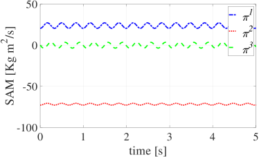
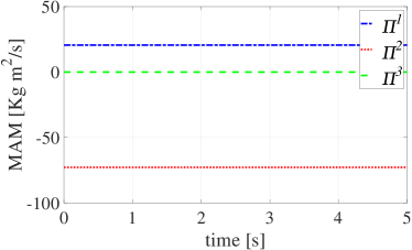
Figure 1: Case 1 - SAM components (left) and MAM components (right).

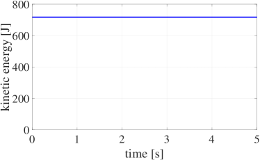
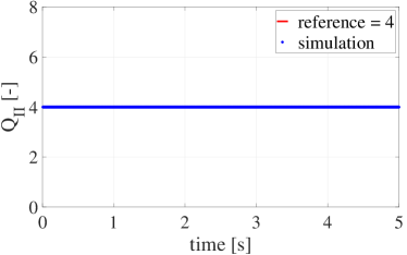
Figure 2: Case 1 - kinetic energy (left) and second quotient of precision (right).

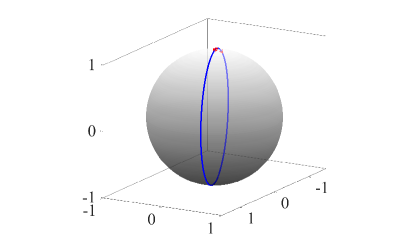
Figure 3: Case 1 - trajectory of $\bm{d}_{3}$ on $S^{2}$.

$t$	$Q_{\mathrm{II}}$
$[$s$]$	$[-]$
$1.000000$	$3.994933$
$2.000000$	$3.994869$
$3.000000$	$3.994787$
$4.000000$	$3.994663$
$5.000000$	$3.994504$

Table 1: Case 1 - second quotient of precision.

$t$	$\mathit{\Pi}^{1}$	$\mathit{\Pi}^{2}$	$K$
$[$s$]$	$[$Kg m2/s$]$	$[$Kg m2/s$]$	$[$J$]$
$1.000000$	$20.571428$	$-72.857142$	$717.428571$
$2.000000$	$20.571428$	$-72.857142$	$717.428571$
$3.000000$	$20.571428$	$-72.857142$	$717.428571$
$4.000000$	$20.571428$	$-72.857142$	$717.428571$
$5.000000$	$20.571428$	$-72.857142$	$717.428571$

Table 2: Case 1 - motion invariants - stationary values.

6.2 Case 2 - response to a vanishing load

For this second case we consider

$$\bm{\mathit{\Lambda}}(0)=\bm{I}\,,\quad\bm{\omega}_{\perp}(0)=\bm{0}\,\,\mathrm{~{}rad/s}$$ (114)

and

$$\bm{m}^{\mathrm{ext}}_{\perp}(t)=-f(t)(2472.5\bm{d}_{1}(t)+1075\bm{d}_{2}(t))\,\,\mathrm{~{}Kgm^{2}/s^{2}},$$ (115)

where

$$f(t)=\left\{\begin{array}[]{ccc}2t&\mathrm{for}&0\leq t<0.5\\ 2-2t&\mathrm{for}&0.5\leq t<1\\ 0&\mathrm{for}&t\geq 1\end{array}\right.$$ (116)

Figure 4 presents the time history for the spatial and material components of the angular momentum, where the applied material load $\bm{m}^{\mathrm{ext}}_{\perp}$ is active only during the first second of simulation. On the left figure, we observe that the components of the spatial angular momentum vary starting from zero since the rotating rigid body is initially at rest. After the load vanishes, the components of the spatial angular momentum oscillate with constant amplitude and frequency and therefore, they are not constant, but indicate a steady state. On the right figure we can observe that the components of the material angular momentum also vary from zero, except the third one that remains always equal to zero. After the material load vanishes, the components of the material angular momenta are identically preserved. Once again, the first and second components are constant and different from zero.

Figure 5 presents the time history for the kinetic energy and the second quotient of precision. On the left, we can observe that the kinetic energy vary during the first second, where the applied material load is active. After this vanishes, the kinetic energy is identically preserved. On the right figure we confirm again that the second quotient of precision is approximately $4$, see also Table 3, which means that the integrator is second-order accurate even during the time in which the applied material load is active.

Figure 6 shows the trajectory followed by $\bm{d}_{3}$, which due to the fixed relation among components of the applied material load takes place on a plane that separates the sphere in two half spheres. Such trajectory minimizes locally the distance on $S^{2}$ and thus, this is geodesic as well. Table 4 presents the stationary values for the motion invariants.

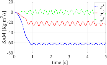
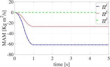
Figure 4: Case 2 - SAM components (left) and MAM components (right).

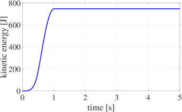
Figure 5: Case 2 - kinetic energy (left) and second quotient of precision (right).

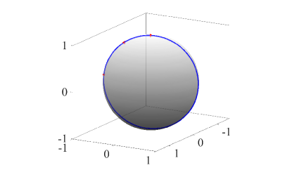
Figure 6: Case 2 - trajectory of $\bm{d}_{3}$ on $S^{2}$.

$t$	$Q_{\mathrm{II}}$
$[$s$]$	$[-]$
$1.000000$	$3.987886$
$2.000000$	$3.985379$
$3.000000$	$3.984407$
$4.000000$	$3.983255$
$5.000000$	$3.981796$

Table 3: Case 2 - second quotient of precision.

$t$	$\mathit{\Pi}^{1}$	$\mathit{\Pi}^{2}$	$K$
$[$s$]$	$[$Kg m2/s$]$	$[$Kg m2/s$]$	$[$J$]$
$1.000000$	$-61.749731$	$-26.845155$	$746.591699$
$2.000000$	$-61.749731$	$-26.845155$	$746.591699$
$3.000000$	$-61.749731$	$-26.845155$	$746.591699$
$4.000000$	$-61.749731$	$-26.845155$	$746.591699$
$5.000000$	$-61.749731$	$-26.845155$	$746.591699$

Table 4: Case 2 - motion invariants - stationary values.

6.3 Case 3 - response to nonzero initial conditions and a vanishing load

For this last case we consider

$$\bm{\mathit{\Lambda}}(0)=\bm{I}\,,\quad\bm{\omega}_{\perp}(0)=1.5\bm{d}_{1}+4.5\bm{d}_{2}\,\,\mathrm{~{}rad/s}$$ (117)

and

$$\bm{m}^{\mathrm{ext}}_{\perp}(t)=-f(t)(1236.25\bm{d}_{1}(t)+537.5\bm{d}_{2}(t))\,\,\mathrm{~{}Kgm^{2}/s^{2}}$$ (118)

with $f(t)$ defined as in Eq. (116).

Figure 7 presents the time history for the spatial and material components of the angular momentum. On the left, we can observe that the components of the spatial angular momentum vary starting from the values corresponding to the initial condition adopted. After the material load vanishes, the components of the spatial angular momentum oscillate with constant amplitude and frequency indicating a steady state. On the right, we observe that the components of the material angular momentum also vary from the values corresponding to the initial condition adopted, except the third one that remains always equal to zero. After the material load vanishes the components of the material angular momenta are identically preserved as in the previous cases.

Figure 8 presents the time history for the kinetic energy and the second quotient of precision. On the left we can observe that the kinetic energy vary during the first second, where the applied material load is active. After this vanishes, the kinetic energy is identically preserved. To the right we see that the second quotient of precision is approximately $4$, see also Table 5.

Figure 9 shows the trajectory followed by $\bm{d}_{3}$. During the first second, the trajectory does not render a distance minimizing curve on $S^{2}$. This is due to the combination of initial condition adopted and the load applied that produces a change in the direction of the axis of rotation. After the material load vanishes, the trajectory describes a circle of radius $1$. Table 6 provides the stationary values for the motion invariants.

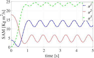
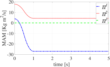
Figure 7: Case 3 - SAM components (left) and MAM components (right).

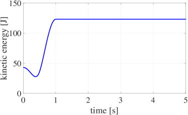
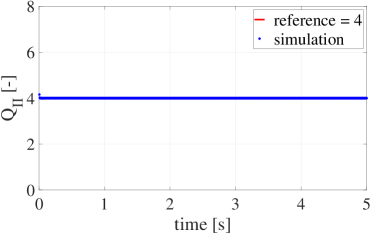
Figure 8: Case 3 - kinetic energy (left) and second quotient of precision (right).

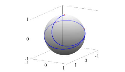
Figure 9: Case 3 - trajectory of $\bm{d}_{3}$ on $S^{2}$.

$t$	$Q_{\mathrm{II}}$
$[$s$]$	$[-]$
$1.000000$	$3.998023$
$2.000000$	$3.997424$
$3.000000$	$3.997327$
$4.000000$	$3.997289$
$5.000000$	$3.997247$

Table 5: Case 3 - second quotient of precision.

$t$	$\mathit{\Pi}^{1}$	$\mathit{\Pi}^{2}$	$K$
$[$s$]$	$[$Kg m2/s$]$	$[$Kg m2/s$]$	$[$J$]$
$1.000000$	$-27.042702$	$4.351472$	$123.059926$
$2.000000$	$-27.042702$	$4.351472$	$123.059926$
$3.000000$	$-27.042702$	$4.351472$	$123.059926$
$4.000000$	$-27.042702$	$4.351472$	$123.059926$
$5.000000$	$-27.042702$	$4.351472$	$123.059926$

Table 6: Case 3 - motion invariants - stationary values.

7 Summary

This article describes the governing equations of the rotating rigid body in a nonholonomic context, and discusses their relation with other, well-known, equivalent models based on rotations and orthonormal vectors. The equations obtained are non-variational and possess first invariants of motion. Some of them, i.e., the nonholonomic momenta (first and second components of the material angular momentum), are neither evident from the standard descriptions nor intuitive. To the best of our knowledge, there is no work in the literature that reports similar observations and thus, it represents a main innovation of the current work.

Complementing the rigorous mathematical analyis done for the proposed model, an implicit, second order accurate, energy and momentum conserving algorithm is presented, which discretizes in time the rigid body, nonholomic equations. Such a time integration scheme preserves exactly the energy and nonholonomic momenta and thus, this represents also a main innovation of the current work. Finally, simple examples, which make use of all elements of the approach proposed, are provided and confirm the excellent conservation properties and second order accuracy of the new scheme.

Appendix A Second quotient of precision

To investigate the correctness of the integration scheme, we can employ the second quotient of precision [43]. Any numerical solution of an initial value problem can be written as

$$\bm{\xi}(t,h,k)=\bm{\xi}(t)+\left(\frac{h}{k}\right)\bm{\psi}_{1}(t)+\left(\frac{h}{k}\right)^{2}\bm{\psi}_{2}(t)+\ldots+\left(\frac{h}{k}\right)^{n}\bm{\psi}_{n}(t)+\mathcal{O}(h^{n+1})$$ (119)

with $\bm{\xi}(t)$ representing the exact solution of the initial value problem under consideration and $\bm{\psi}_{i}$ for $i=1,\ldots,n$ representing smooth functions that only depend on the time parameter $t$. $h$ stands for the time step and $k$ is a positive integer number that enables defining finer solutions computed from the original resolution.

Let us introduce the second quotient of precision given by

$$Q_{\textrm{II}}(t)=\frac{\left\|\bm{\xi}(t,h,1)-\bm{\xi}(t,h,2)\right\|}{\left\|\bm{\xi}(t,h,2)-\bm{\xi}(t,h,4)\right\|}\,.$$ (120)

For the numerator, we have that

$$\left\|\bm{\xi}(t,h,1)-\bm{\xi}(t,h,2)\right\| =\left\|\left(\frac{h}{1}\right)^{n}\bm{\psi}_{n}(t)-\left(\frac{h}{2}\right)^{n}\bm{\psi}_{n}(t)+\mathcal{O}(h^{n+1})\right\|$$ (121)

$$=\left(\frac{2^{n}-1}{2^{n}}\right)h^{n}\left\|\bm{\psi}_{n}(t)\right\|+\mathcal{O}(h^{n+1})$$

meanwhile, for the denominator, we have that

$$\left\|\bm{\xi}(t,h,2)-\bm{\xi}(t,h,4)\right\| =\left\|\left(\frac{h}{2}\right)^{n}\bm{\psi}_{n}(t)-\left(\frac{h}{4}\right)^{n}\bm{\psi}_{n}(t)+\mathcal{O}(h^{n+1})\right\|$$ (122)

$$=\left(\frac{2^{n}-1}{4^{n}}\right)h^{n}\left\|\bm{\psi}_{n}(t)\right\|+\mathcal{O}(h^{n+1})\,.$$

If we have time steps that are sufficiently small, it can be showed that the second quotient of precision is very close to take the value $2^{n}$, i.e.,

$$Q_{\textrm{II}}(t)=\frac{\left(\frac{2^{n}-1}{2^{n}}\right)h^{n}\left\|\bm{\psi}_{n}(t)\right\|+\mathcal{O}(h^{n+1})}{\left(\frac{2^{n}-1}{4^{n}}\right)h^{n}\left\|\bm{\psi}_{n}(t)\right\|+\mathcal{O}(h^{n+1})}=2^{n}+\mathcal{O}(h^{n+1})\approx 2^{n}\,.$$ (123)

In this work, we consider an integration algorithm whose accuracy is warranted to be of second order and thus, $Q_{\textrm{II}}(t)\approx 4$. Be aware that for the computation of precision quotients, $h$ needs to be chosen small enough. Such a selection strongly depends on the case considered. Moreover, when $\|\bm{\psi}_{n}(t)\|$ is very small, the test may fail even if correctly implemented. Therefore, we recommend to play with initial conditions and time resolutions for achieving correct pictures.

References

• [1] H. Goldstein, Classical Mechanics. Addison-Wesley, 2nd ed., 1980.
• [2] V. I. Arnold, Mathematical methods of classical mechanics. Springer, 1989.
• [3] J. C. Simo, J. E. Marsden, and P. S. Krishnaprasad, “The Hamiltonian structure of nonlinear elasticity: the material and convective representations of solids, rods, and plates,” Archive for Rational Mechanics and Analysis, vol. 104, pp. 125–183, 1988.
• [4] S. S. Antman, Nonlinear problems of elasticity. New York: Springer, 1995.
• [5] A. Mielke and P. Holmes, “Spatially complex equilibria of buckled rods,” Archive for Rational Mechanics and Analysis, vol. 101, pp. 319–348, 1988.
• [6] J. C. Simo and K. K. Wong, “Unconditionally stable algorithms for rigid body dynamics that exactly preserve energy and momentum,” International Journal for Numerical Methods in Engineering, vol. 31, pp. 19–52, 1991.
• [7] I. Romero, “Formulation and performance of variational integrators for rotating bodies,” Computational Mechanics, vol. 42, pp. 825–836, 2008.
• [8] J. C. Simo and L. Vu-Quoc, “A three-dimensional finite-strain rod model. Part II: Computational aspects,” Computer Methods in Applied Mechanics and Engineering, vol. 58, pp. 79–116, 1986.
• [9] C. Sansour and H. Bednarczyk, “The Cosserat surface as a shell model, theory and finite-element formulation,” Computer Methods in Applied Mechanics and Engineering, vol. 120, pp. 1–32, 1995.
• [10] G. Jelenić and M. A. Crisfield, “Interpolation of rotational variables in nonlinear dynamics of 3d beams,” International Journal for Numerical Methods in Engineering, vol. 43, pp. 1193–1222, 1998.
• [11] I. Romero and F. Armero, “Numerical integration of the stiff dynamics of geometrically exact shells: an energy-dissipative momentum-conserving scheme,” International Journal for Numerical Methods in Engineering, vol. 54, pp. 1043–1086, 2002.
• [12] P. Betsch and P. Steinmann, “Constrained dynamics of geometrically exact beams,” Computational Mechanics, vol. 31, pp. 49–59, 2003.
• [13] I. Romero and M. Arnold, “Computing with rotations: algorithms and applications,” in Encyclopedia of Computational Mechanics (E. Stein, R. de Borst, and T. J. R. Hughes, eds.), John Wiley & Sons, 2017.
• [14] I. Romero and F. Armero, “An objective finite element approximation of the kinematics of geometrically exact rods and its use in the formulation of an energy-momentum conserving scheme in dynamics,” International Journal for Numerical Methods in Engineering, vol. 54, pp. 1683–1716, 2002.
• [15] P. Betsch and P. Steinmann, “Frame-indifferent beam finite elements based upon the geometrically exact beam theory,” International Journal for Numerical Methods in Engineering, vol. 54, pp. 1775–1788, 2002.
• [16] P. Betsch and S. Leyendecker, “The discrete null space method for the energy consistent integration of constrained mechanical systems. Part II: Multibody dynamics,” International Journal for Numerical Methods in Engineering, vol. 67, pp. 499–552, 2006.
• [17] R. L. Bishop, “There is more than one way to frame a curve,” The American Mathematical Monthly, vol. 82, pp. 246–251, 1975.
• [18] Y. Shi and J. E. Hearst, “The Kirchhoff elastic rod, the nonlinear Schrödinger equation, and DNA supercoiling,” The Journal of Chemical Physics, vol. 101, pp. 5186–5200, 1994.
• [19] T. McMillen and A. Goriely, “Tendril perversion in intrinsically curved rods,” Journal Nonlinear Science, vol. 12, pp. 241–281, 2002.
• [20] B. Audoly, N. Clauvelin, and S. Neukirch, “Elastic knots,” Physical Review Letters, vol. 99, pp. 137–4, 2007.
• [21] I. Romero and C. G. Gebhardt, “Variational principles for nonlinear Kirchhoff rods,” Acta Mechanica, 2019.
• [22] P. Betsch, “Energy-consistent numerical integration of mechanical systems with mixed holonomic and nonholonomic constraints,” Computer Methods in Applied Mechanics and Engineering, vol. 195, pp. 7020–7035, 2006.
• [23] K. R. Hedrih, “Rolling heavy ball over the sphere in real Rn3 space,” Nonlinear Dynamics, vol. 97, pp. 63–82, 2019.
• [24] T. Lee, M. Leok, and N. H. McClamroch, “Lagrangian mechanics and variational integrators on two-spheres,” International Journal for Numerical Methods in Engineering, vol. 79, pp. 1147–1174, 2009.
• [25] T. Lee, M. Leok, and N. H. McClamroch, Global Formulations of Lagrangian and Hamiltonian Dynamics on Manifolds. Springer International Publishing, 2018.
• [26] R. I. McLachlan, G. R. W. Quispel, and N. Robidoux, “Geometric integration using discrete gradients,” Philosophical Transactions of the Royal Society of London. Series A. Mathematical, Physical Sciences and Engineering, vol. 357, pp. 1021–1045, 1999.
• [27] E. Celledoni, V. Grimm, R. I. McLachlan, D. I. McLaren, D. O’Neale, B. Owren, and G. R. W. Quispel, “Preserving energy resp. dissipation in numerical PDEs using the ‘Average Vector Field’ method,” Journal of Computational Physics, vol. 231, pp. 6770–6789, 2012.
• [28] C. G. Gebhardt, I. Romero, and R. Rolfes, “A new conservative/dissipative time integration scheme for nonlinear mechanical systems,” Computational Mechanics, 2019.
• [29] J. E. Marsden and T. S. Ratiu, Introduction to Mechanics and Symmetry. New York: Springer, first ed., 1994.
• [30] M. Eisenberg and R. Guy, “A proof of the hairy ball theorem,” The American Mathematical Monthly, vol. 86, pp. 571–574, 1979.
• [31] J. C. Simo and D. D. Fox, “On a stress resultant geometrically exact shell model. I. Formulation and optimal parametrization,” Computer Methods in Applied Mechanics and Engineering, vol. 72, pp. 267–304, 1989.
• [32] I. Romero, “The interpolation of rotations and its application to finite element models of geometrically exact rods,” Computational Mechanics, vol. 34, pp. 121–133, 2004.
• [33] I. Romero, M. Urrecha, and C. J. Cyron, “A torsion-free nonlinear beam model,” International Journal of Non-Linear Mechanics, vol. 58, pp. 1–10, 2014.
• [34] S. Hosseini and A. Uschmajew, “A Riemannian gradient sampling algorithm for nonsmooth optimization on manifolds,” SIAM Journal on Optimization, vol. 27, pp. 173–189, 2017.
• [35] R. Bergmann, J. H. Fitschen, J. Persch, and G. Steidl, “Priors with coupled first and second order differences for manifold-valued image processing,” Journal of Mathematical Imaging and Vision, vol. 60, pp. 1459–1481, 2018.
• [36] E. Hairer, C. Lubich, and G. Wanner, Geometric numerical integration. Berlin: Springer, 2nd ed., 2006.
• [37] J. Langer and D. Singer, “Lagrangian aspects of the Kirchhoff elastic rod,” SIAM Review, vol. 38, pp. 605–618, 1996.
• [38] R. T. Farouki, “Rational rotation-minimizing frames–recent advances and open problems,” Applied Mathematics and Computation, vol. 272, pp. 80–91, 2016.
• [39] I. Romero and F. Armero, “An objective finite element approximation of the kinematics of geometrically exact rods and its use in the formulation of an energy-momentum conserving scheme in dynamics,” International Journal for Numerical Methods in Engineering, vol. 54, pp. 1683–1716, 2002.
• [40] J. C. Simo and N. Tarnow, “The discrete energy-momentum method. conserving algorithms for nonlinear elastodynamics,” Zeitschrift für Angewandte Mathematik und Physik, vol. 43, pp. 757–792, 1992.
• [41] C. G. Gebhardt, B. Hofmeister, C. Hente, and R. Rolfes, “Nonlinear dynamics of slender structures: a new object-oriented framework,” Computational Mechanics, vol. 63, pp. 219–252, 2019.
• [42] C. G. Gebhardt, M. C. Steinbach, and R. Rolfes, “Understanding the nonlinear dynamics of beam structures: a principal geodesic analysis approach,” Thin-Walled Structures, vol. 140, pp. 357–372, 2019.
• [43] H.-O. Kreiss and O. E. Ortiz, Introduction to numerical methods for time dependent differential equations. Wiley, 2014.