Table-to-Text Natural Language Generation with Unseen Schemas

Abstract

Traditional table-to-text natural language generation (NLG) tasks focus on generating text from schemas that are already seen in the training set. This limitation curbs their generalizabilities towards real-world scenarios, where the schemas of input tables are potentially infinite. In this paper, we propose the new task of table-to-text NLG with unseen schemas, which specifically aims to test the generalization of NLG for input tables with attribute types that never appear during training. To do this, we construct a new benchmark dataset for this task. To deal with the problem of unseen attribute types, we propose a new model that first aligns unseen table schemas to seen ones, and then generates text with updated table representations. Experimental evaluation on the new benchmark demonstrates that our model outperforms baseline methods by a large margin. In addition, comparison with standard data-to-text settings shows the challenges and uniqueness of our proposed task.

1 Introduction

Over the past few years, table-to-text natural language generation has received increasingly more attention. Typically, table-to-text generation model takes in a table as input and aims to generate a description of its content in natural language as in the example given in figure 1. A table consists of several attribute-value pairs. In this work, we refer to the combination of various attributes that appear in one table as schema. The task of table-to-text generation requires the ability to first understand the information conveyed by the table and then generate fluent natural language to describe the information. Great potential lies in utilizing table-to-text techniques in real-world applications such as question answering, automatic news writing, and task-oriented dialog system.

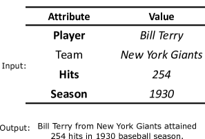
Figure 1: An example of table-to-text generation from Wikipedia. Given a table as the input, we aim to generate a description of the contents of the table. In this work, we tackle a critical challenge in table-to-text generation unseen attribute types (highlighted in bold) appear in the testing scenarios.

A wide range of table-to-text tasks and datasets have been proposed over the past few years such as weathergov Belz (2008), wikibio Lebret et al. (2016), and the E2E challenge Novikova et al. (2017). However, these existing tasks are designed for specific domains with limited attribute types and simple schema patterns. For instance, the E2E dataset Novikova et al. (2017) constructed for restaurant domain has only 8 predefined attribute types and the weathergov Belz (2008) designed for automatic weather report generation has only 10. A notable exception is the wikibio dataset Lebret et al. (2016) that has approximately 7K attribute types. However, most of its instances follow the template of biography, which puts more emphasis on monotonous information such as names, birth dates, and occupations. Although currently prevalent data-driven end-to-end models Bao et al. (2018); Liu et al. (2018); Gardent et al. (2017) yield promising results on these tasks, they implicitly bias towards fixed schema-utterance pairs. Such bias limits their generalizabilities towards real-world scenarios where various unseen attribute types may appear in the input tables.

Therefore, we introduce the new task of table-to-text generation for unseen schemas, where we focus on generating descriptions for input table with schemas that never appear during training. Since previous close-domain table-to-text tasks has little room for generalization, we choose to conduct our experiments on the open-domain dataset wikitabletext Bao et al. (2018) collected from the entire Wikipedia without being restricted to any specific domains. The abundance and diversity of its attribute types and schemas make it possible for us to control the proportion of unseen attributes during the testing phase through subsampling the training set and construct a proper benchmark for our task.

In parallel, conventional methods Konstas and Lapata (2013); Moryossef et al. (2019); Ma et al. (2019) deal with table-to-text task in a two-stage (namely content planning and surface realization) manner. By such means, table understanding and text generation are separated, and the result of text generation is explicitly conditioned on the result of content planning. This quality paves the way to tackling with unseen input table schemas by controlling over their representations while avoiding undermining the reliability of the text generation part.

In light of the points raised above, we propose a novel table-to-text model, AlignNet, which explicitly learns an alignment between unseen schemas with seen ones. Our method is by nature a two-stage model while maintaining the property to be trained end-to-end. When the model receives an unseen table schema as input, it first infers possible alignments with seen schemas in the train set. Then, representations of unseen attribute types are replaced with best aligned seen ones. In a nutshell, our work has the following contributions:

• We propose the new task of table-to-text natural language generation for unseen schemas. Compared with traditional table-to-text tasks, the new task is closer to real-world scenarios.

• In order to deal with the new problem, we propose a novel end-to-end neural model that explicitly learns to align unseen schemas to seen ones.

• We construct a benchmark dataset for this new task and demonstrate the effectiveness and capability of our method to deal with unseen table schemas.

2 Related Work

2.1 Data-to-Text Generation

Data-to-text generation is a vibrant subdomain of natural language generation, alongside a wide range of fields such as machine translation Kalchbrenner and Blunsom (2013); Bahdanau et al. (2014), document summarization Rush et al. (2015); Gu et al. (2016); See et al. (2017), and dialog system Vinyals and Le (2015); Shang et al. (2015); Li et al. (2016). The speciality of table-to-text generation is, by definition, non-linguistic input Reiter and Dale (1997); Konstas and Lapata (2013). Traditionally, data-to-text generation systems are implemented in a two-stage manner. The first core step determines what to say (content planning) and the second step determines how to say (surface realization). Earlier surface realization models focus on generating natural language from rules and hand-crafted templates Reiter et al. (2005); Dale et al. (2003), meaning representation language (MRL) Wong and Mooney (2007), probabilistic context-free grammar (PCFG) Cahill and van Genabith (2006), etc. Later, end-to-end unified models Angeli et al. (2010); Konstas and Lapata (2013) that combine the two steps by joint optimization became prevalent.

The trend of merging content planning and surface realization became even stronger since the introduction of sequence-to-sequence framework Sutskever et al. (2014). A number of improvements upon sequence-to-sequence framework such as copy mechanism Bao et al. (2018), attention mechanism Liu et al. (2018), symbolic reasoning Nie et al. (2018) have been explored. In the meantime, attempts Puduppully et al. (2018) that aim to decompose sequence-to-sequence framework into content planning and surface realization without sacrificing the end-to-end trainable property have yielded promising results. Nevertheless, most previous studies are conducted in closed-world settings that focus on limited input attribute types and schemas and pay little attention to generalizability.

2.2 Domain Adaptation and Zero-Shot Learning

Domain adaptation typically involves adapting models trained on rich-resource domains to low-resource domains. Recent years have seen growing efforts on domain adaptation for NLG tasks, such as machine translation Hu et al. (2019), dialog systems Qian and Yu (2019). In terms of data-to-text generation, Angeli et al. Angeli et al. (2010) first propose a unified domain-independent framework that does not require domain-specific feature engineering. Wen et al. Wen et al. (2016) manually create ontologies for different domains and leverage data augmentation technique to adapt a data-to-text generation system to multiple domains.

Meanwhile, zero-shot learning can be regarded as a special case of transfer learning, where no label information of the target domain can be obtained during learning. In prior work, zero-shot learning has been studied for question generation Elsahar et al. (2018), image captioning Wang et al. (2018), dialog generation Zhao and Eskenazi (2018), etc.

Our proposed task bears some similarities to domain adaption and zero-shot learning in the way that the evaluation is conducted on test sets which contain unseen attribute types and the distribution of data during the testing phase is different from that during the training phase.

On the other hand, the proposed task is different from standard domain adaptation since we do not explicitly define domains such as restaurant, sports, biography in our task. Our main focus is to evaluate the generalizability towards any given schema rather than another specific domain. Thus, it is not necessary to obtain the domain-specific knowledge from external resources that is required in most zero-shot learning and domain adaptation methods Wen et al. (2016); Zhao and Eskenazi (2018).

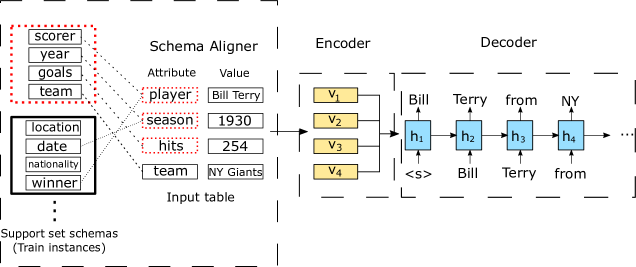
Figure 2: The overall architecture of our model. Attention and copy mechanism are omitted for simplicity. Unseen attribute types (player, season, hits) of the input table are in dotted red boxes. The schema aligner first computes alignment scores for each support set schema and select the schema with the highest alignment score (the one in dotted red box) to replace the paired attribute representations. The encoder then takes in the updated representations as input. During training, we sample the support set from the training set excluding the current training instance. During testing, the support set is sampled from the whole training set.

3 Task Definition

In this section, we first describe the formalization of general table-to-text tasks and then introduce the new task of table-to-text generation for unseen schemas.

3.1 Formalization of Table-to-Text

Provided with a table $T$ as the input, the table-to-text generation task aims to generate a natural language sequence $\mathbf{y}=\{y_{1},y_{2},\cdots,y_{m}\}$ that describes the content of $T$ as output. In this work, a table $T$ is defined as a list of $n$ attribute-value pairs $\{a_{i}:c_{i}\}^{n}_{i=1}$.

3.2 Table-to-Text Generation for Unseen Schemas

Traditional table-to-text generation tasks and datasets put little emphasis on evaluating the performance on unseen schemas. In real-world applications, however, the types of attributes are not limited to those that appear during training. Thus, these traditional table-to-text tasks has limited generalizability towards real-world scenarios.

In view of the weakness mentioned above, we propose the new task of table-to-text generation from unseen schemas. Unlike traditional settings, the new task imitates open-world scenarios. It explicitly aims to generate texts from schemas with a large proportion of attribute types that never appear in the training set.

4 Our Framework

4.1 Table-to-Sequence Framework

Our model is based on the state-of-the-art table-to-sequence framework proposed in Bao et al. (2018). Their method is by nature an encoder-decoder model which first encodes an input table into a vector representation and then decodes it into a natural language sequence. In the course of decoding, attention mechanism and copy mechanism are leveraged in order to generate accurate .

4.1.1 Table Encoder Module

First, the model embeds attribute types and cell contents into vector representations. Specifically, each attribute $a_{i}$ is represented as a vector $\mathbf{e}_{i}^{a}$ and its corresponding content cell $c_{i}$ is represented as a vector $\mathbf{e}_{i}^{c}$. Afterwards, we compute the final representation of an attribute-value pair using $\mathbf{v}_{i}=\mathrm{FFN}_{e}([e_{i}^{a};e_{i}^{c}])$, where $[\,;\,]$ is the concatenation operator and $\mathrm{FFN}_{e}$ is a single-layer feedforward neural network.

Then, a vector $\mathbf{h}_{0}$ representing the whole table is computed by a sequence-to-vector encoder $\mathbf{h}_{0}=f_{enc}(\langle\mathbf{v}_{1},\mathbf{v}_{2},\cdots,\mathbf{v}_{n}\rangle)$ and utilized to initialize the decoder state.

4.1.2 Decoder Module

The model decoder utilizes copy mechanism Gu et al. (2016) that is capable of copying tokens from both table attributes and cell contents. At decoding step $t$, an LSTM-based decoder takes in the predicted token representation output $\mathbf{y}_{t-1}$ of step $t-1$, the hidden state $\mathbf{h}_{t-1}$ of step $t-1$, and an attentive vector $\mathbf{m}_{t}$ as inputs. The recurrence of decoding procedure is given by

$$h_{t}=f_{dec}(\mathbf{y}_{t-1},\mathbf{h}_{t-1},\mathbf{m}_{t})$$ (1)

$$\mathbf{m}_{t}=\sum_{i=1}^{n}\alpha_{ti}\mathbf{v}_{i};\;\;\alpha_{ti}=\frac{exp(\eta(\mathbf{m}_{t-1},\mathbf{v}_{i}))}{\sum_{j=1}^{n}exp(\eta(\mathbf{m}_{t-1},\mathbf{v}_{j}))}$$ (2)

where $\mathbf{v}_{i}$ is the representation of the $i$-th table cell and $\eta(\cdot,\cdot)$ is a bilinear attention function. Decoder output $\mathbf{h}_{t}$ of step $t$ is then fed into a word prediction layer to determine a generation score for each word in the vocabulary.

With regard to copy mechanism, a copy score $g_{i}^{a}$ for attribute and a copy score $g_{i}^{c}$ for cell content is computed for each attribute-value pair of the input table $T$ by

$$g_{i}^{a} =\mathrm{FFN}_{g^{a}}([\mathbf{y}_{t-1};\mathbf{h}_{t};\mathbf{m}_{t};\mathbf{v}_{i};\mathbf{e}_{i}^{a}]);$$ (3)

$$g_{i}^{c} =\mathrm{FFN}_{g^{c}}([\mathbf{y}_{t-1};\mathbf{h}_{t};\mathbf{m}_{t};\mathbf{v}_{i};\mathbf{e}_{i}^{c}]).$$

The generation scores and copy scores are then concatenated and fed into a $\mathrm{softmax}$ function to calculate the final probability distribution over the vocabulary set extended with input table contents.

4.2 Table Alignment and Attribute Representation Replacement

To address the challenge presented by unseen schemas during the test phase, we begin with the intuition that different tables may share some common fields of contents even though they have different schemas. For instance, tables that describe sport game events often use “season” while tables that describe general historical events usually use “year” to represent the attribute of time. Another example is that tables may use various types of words such as “player”, “winner”, “actor” in terms of the attribute of person. Therefore, it is reasonable to seek for possible paraphrases within the training set when the table-to-text model encounters unseen attribute types during testing.

Input: Table $T^{S}$ from support set with attribute representations $\{\mathbf{v}_{j}^{S}\}_{j=1}^{m}$ ; input table $T$ with attribute representations $\{\mathbf{v}_{i}\}_{i=1}^{n}$

Output: Alignment score $r$ ; Alignment $\{(i,j_{i})\}_{i=1}^{n}$.

1

2Calculate similarity matrix $\mathbf{S}=\{s_{ij}=\frac{\mathbf{v}_{i}\mathbf{v}_{j}^{S}}{\lvert\mathbf{v}_{i}\rvert\lvert\mathbf{v}_{j}^{S}\rvert}\}_{n\times m}$;

3

4Use the Hungarian Algorithm to find an optimal alignment $\{(i,j_{i})\}_{i=1}^{n}$ that maximizes the sum of similarity scores;

5

6Discard alignment pairs $\{(i,j_{i})\}$ where $s_{ij_{i}}<0$; Compute alignment score using $r=\sum_{i=1}^{n}s_{ij_{i}}$.

Algorithm 1 Schema Alignment

In this section, we propose an end-to-end model that explicitly learns to align unseen table schemas with seen ones. An overview of the architecture is shown in figure 2. As illustrated, the main difference between our model and the traditional end-to-end table-to-sequence model lies on the encoder side.

First, for each input table, the model randomly samples a support set $S=\{T^{S}_{1},T^{S}_{2},\cdots,T^{S}_{k}\}$ from the train set and encodes attribute representations $\mathbf{v}_{i_{j}^{S}}$ for each table $T^{S}_{i}$ in $S$. Then, the model computes an alignment score $r$ for each table using algorithm 1. The core step of algorithm 1 is the application of the Hungarian Algorithm Kuhn (1955) designed for bipartite graph matching. It is based on the property that if a number is added or subtracted from all of the elements of one row or one column, the optimal alignment of the resulting matrix is still an optimal alignment of the original matrix. By reducing some matrix elements to zeros and keeping other elements negative, the algorithm searches for an optimal alignment within the positions of zeros. The searching process is performed by iterating over rows and columns. Note that the cosine similarity between two vectors can be negative and the last step allows mismatch when no satisfactory alignments could be found for an input attribute.

After we find the highest alignment score $r$ and its associated best alignment $\{(i,j_{i})\}_{i=1}^{n}$, attribute representation $\mathbf{e}^{a}_{i}$ of the input table is then replaced by attribute representation $\mathbf{e}_{j_{i}}^{S,a}$ from the support set schema. The later steps then follow the traditional table-to-sequence framework discussed in the previous section.

4.3 Learning

Our model is trained in an end-to-end fashion to maximize the log-likelihood of the gold output text sequence. The negative log-likelihood loss for a single training instance $(T,\mathbf{y})\in\mathcal{D}$ is defined as:

$$L_{\mathrm{NLL}}=-\log p(\mathbf{y}|T,\boldsymbol{\theta})$$ (4)

where $\boldsymbol{\theta}$ denotes the model parameters.

Meanwhile, in order to provide guidance for better schema alignment, an additional loss term that take an alignment score $r$ into consideration is adopted. The final loss is denoted as

$$L=\sum_{\mathcal{D}}\left(L_{\mathrm{NLL}}+\lambda rL_{\mathrm{NLL}}\right).$$ (5)

where $\lambda$ is a positive scalar hyperparameter.

The rationale of the modified loss term is to minimize the gradient when an input table is aligned to an unsatisfactory schema with relatively low alignment score. On the other hand, when $L_{\mathrm{NLL}}$ is relatively high (which means the aligned schema cannot help to generate the expected output sequence), the loss term encourages the model to yield a lower alignment score.

5 Experiments

Model	50			100			200			500
	Test	Dev		Test	Dev		Test	Dev		Test	Dev
Base	14.1	14.5		14.8	14.3		16.0	16.1		17.7	18.3
Base+targ-copy	13.2	13.3		15.7	15.5		15.7	15.5		18.6	17.9
Base+MAML	9.9	9.8		11.7	12.0		16.6	16.3		18.4	18.7
AlignNet	18.8	19.3		18.7	18.8		18.7	18.5		21.0	20.6

Table 1: Comparison of results on the benchmark dataset. We report BLEU-4 scores on training set sizes of 50, 100, 200, 500 with unseen attribute proportion above 80%. The results are averaged over 10 randomly sampled train sets for each size.

Model	50			100			200			500
	Test	Dev		Test	Dev		Test	Dev		Test	Dev
Base	18.9	19.0		23.2	23.3		22.3	23.8		23.7	25.5
Base+targ-copy	12.9	13.0		12.5	12.0		16.0	16.2		22.0	21.7
Base+MAML	10.7	10.8		16.6	17.1		21.7	22.5		26.7	25.5
AlignNet	23.4	22.1		24.8	25.0		26.3	25.4		26.5	25.6

Table 2: Comparison of results on the datasets with traditional settings that directly samples from the train set. In the same vein as table 1, we report the average scores over 10 randomly sampled for each training set size.

In this section, we first describe a benchmark dataset that we construct for the new task of table-to-text generation for unseen schemas. Then, we show the experimental results of our model and several other baselines on the benchmark dataset. Some qualitative analysis will be provided at last.

5.1 Dataset

Our benchmark dataset is constructed based on the wikitabletext dataset Bao et al. (2018). wikitabletext is an open-domain table-to-text dataset collected from the whole Wikipedia, which means the table schemas are not restricted to any specific domains. Table 3 shows some important statistics of this dataset. Compared with previous close-domain datasets such as robocup Chen and Mooney (2008), rotowire Wiseman et al. (2017) and wikibio Lebret et al. (2016), wikitabletext has the most diverse attribute types that are suitable to test the generalizability of table-to-text models.

Type	Value
#Instances	13.3K
#Tokens	185.0K
#Attribute Types	3.0K
Average Length	13.9
#Attribute per Table	4.1

Table 3: Statistics of the wikitabletext dataset.

Using the original train/development/test split setup of wikitabletext, about 98% of the attribute types of development set and test set are seen during training. Thus, we keep the original development and test set and subsample the train set in order to limit the number of seen attribute types. To be more specific, we sample train set of size 50, 100, 200, and 500 while keeping the proportion of unseen attribute types in development and test set to be over 80%. To rule out the impact of randomness with regard to the choice of training instances, we randomly sampled 10 sets for each size.

5.2 Implementation Details

To deal with the problem of out-of-vocabulary words, we use 50-dimensional pretrained GloVe word vector Pennington et al. (2014) as pretrained token embeddings. During training, we freeze the embeddings of words to maintain the semantics and allow other neural network parameters to be trainable. The hidden state size of $\mathrm{FFN}_{e}$ is set as 100. For the sequence-to-vector encoder, we use a bi-directional LSTM with a hidden state size of 100. We set the decoder hidden state size to be 200 and output token embedding size to be 25. The support set size is set to 25 for train set size 50 and 50 for train set size 100, 200, and 500. As for the vocabulary, we aim to generate words that appear more than 10 times in the training set. We use AdaDelta optimizer to adaptively change the learning rate from $1.0$. The hyperparameter in the loss term $\lambda$ is set to $0.01$.

During decoding, we feed a special token $\langle s\rangle$ into the decoder in the beginning. We stop the generation process when a special ending token $\langle e\rangle$ is output or the length of the sequence exceeds 20. We apply beam search Sutskever et al. (2014); Bahdanau et al. (2014) of size 5 for all the models. In terms of the evaluation metric, we use BLEU-4 Papineni et al. (2002) which is a widely adopted metric in natural language generation tasks.

5.3 Baselines

5.3.1 Base

We first implemented the state-of-the-art model from Bao et al. (2018) and denote it as Base. The architecture of Base is the same with as the one shown in figure 2 without schema aligner module.

5.3.2 Base+targ-copy

Inspired by the work of Hashimoto et al., we implement a model that retrieves the most similar instance from train set and generates a textual sequence $\mathbf{y}$ conditioning on the input table $T$ and retrieved instance $(T^{\star},\mathbf{y}^{\star})$. The model is implemented with extended copy mechanism that could copy from $\mathbf{y}^{\star}$.

5.3.3 Base+MAML

Inspired by the success of applying meta-learning method to text-to-SQL task Huang et al. (2018), we implemented a MAML-based Finn et al. (2017) framework for table-to-text NLG with pseudo-tasking Huang et al. (2018). We use bag-of-embedding of attributes to calculate similarity scores between tables and construct a pseudo-task that consists of top-5 similar instances for each input instance. The pseudo-tasks then serve as the support sets of MAML.

5.4 Experimental Results

We conduct experiments on the benchmark dataset introduced previously. Models are trained on train sets of different sizes and evaluated on the original development and test set. Following previous work, we use BLEU-4 as an automatic evaluation metric. Evaluation results averaged over 10 randomly sampled sets are reported in table 1.

In order to get a better understanding of the challenges presented by the proposed task, we furthermore compare it with a conventional setup which puts no limits on unseen attribute proportion. Training dataset sizes are set to 50, 100, 200, 500 without controlling the number of unseen attribute types. All the results listed in table 2 are averaged over 10 randomly sampled training datasets of each size.

First of all, it can be seen from the results that our AlignNet model gives better or comparable performance other baseline models on most of the datasets not only under the unseen schema settings but also the traditional settings. Second, the comparison between the results of table 1 and table 2 shows that the prevalence of unseen schemas during testing brings more challenges than traditional table-to-text settings to the models. Moreover, it can be seen from the results that AlignNet outperforms other baselines by a large margin when the train set size is 50, 100, 200 and 500 (33.3%, 26.3%, 16.8%, 18.6%) relative improvement under unseen settings, 23.8%, 6.8%, 17.9%, 11.8% under traditional settings).

5.5 Ablation Study

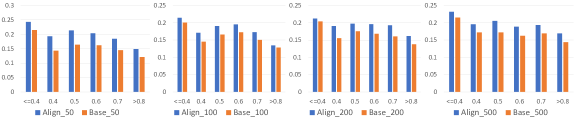
Figure 3: Development set BLEU-4 scores by varying different unseen attribute proportions. We calculate the average score of instances with certain unseen attribute portions. The X axis is unseen attribute proportion and the Y axis is the BLEU-4 score. For example, on the X axis, 0.5 refers to the average score of all development set instances with 50%-60% unseen attributes.

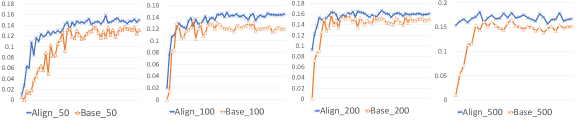
Figure 4: Learning curves (BLEU-4) of the first 50 epochs of the Base model and AlignNet.

5.5.1 Performance on Different Unseen Attribute Proportions

To examine how the amount of unseen attributes in a table affects the performance of our model, we report the performance by various unseen proportions. As demonstrated in figure 3, the AlignNet model shows the most noticeable improvements compared with the Base model for input table schemas with 40%-70% unseen attributes. At the same time, limited improvement is shown for instances with less than 40% unseen attributes, which indicates that the AlignNet works best for tables with a moderate proportion of unseen attribute types.

5.5.2 Learning Curve

Figure 4 shows the learning curves of the AlignNet and the Base model on the development set. We plot the averaged BLEU-4 scores over 10 sampled datasets of each size for the first 50 training epochs. As illustrated in figure 4, AlignNet converges faster than the Base model. We hypothesize that the AlignNet better leverages the information of the training set by explicitly learning an alignment between schemas and directly copy the representations of attributes. Thus, AlignNet requires much smaller efforts to learn a generalizable representation for unseen schemas.

5.6 Qualitative Analysis

5.6.1 Generation Example

Attribute	Value
$\star$Year	1985
$\star$Winner	Peter Glover
$\star$Car	Cheetah mk 8 Volkswagen
Team	Peter Macrow
Gold reference: Peter Glover was from team Peter Macrow.
Generated texts
Base: Peter Glover was <unk ><unk > Peter Macrow.
AlignNet: Peter Glover was from team Peter Macrow.

Attribute	Value
$\star$Name	Ivan Cleary
$\star$Seasons	1996-1999
$\star$Points	722
Gold reference: Ivan Cleary got 722 points during 1996-1999 season.
Generated texts
Base: 722 <unk> 722 in 1996-1999.
AlignNet: In 1996-1999 season, Ivan Cleary got 722 points.

Table 4: Comparison of generated samples between our AlignNet and the Base model. ‘$\star$’ denotes unseen attribute types during training.

Test Attribute	Train Attribute
$\star$Year	Season
$\star$Winner	Rider
$\star$Car	-
Team	Team
$\star$Name	Player
$\star$Seasons	Season
$\star$Points	Goals

Table 5: Aligned train set schemas found by AlignNet for the two examples in 4. ‘$\star$’ denotes unseen attribute types during training.

Table 4 shows two generated examples of the AlignNet and the Base model trained with a dataset of size 200. Due to the presence of unseen attributes, the Base model fails to generate correct textual descriptions for the input tables and tends to generate out-of-vocabulary tokens ($\textless{}unk\textgreater{}$). While the AlignNet correctly selects the contents that needs need to be said and verbalizes them in a sensible way.

5.6.2 Schema Alignment Example

Additionally, we show the schema alignments yielded for the generated examples by the AlignNet model in table 5. For the first input, the model successfully finds a schema consists of attribute “season” and “rider” and matches them with unseen attributes “year” and “winner”. Since we allow mismatch during aligning, attribute “car” has no corresponding attribute and its representation is, therefore, left unchanged. For the second input, all the unseen attributes are aligned to seen ones that represent similar content fields.

6 Conclusion and Future Work

In this paper, we propose the novel task of table-to-text generation for unseen schemas which especially focuses on testing the ability to generalize. In order to solve the problem of unseen schemas, we propose the AlignNet which explicitly aligns unseen schemas to seen ones in the train set to get a better representation of the table. To evaluate the performance of different methods on this new task, we construct a benchmark dataset and conduct extensive experiments.

In future work, we intend to explore more structural information such as latent categorical variables and co-occurrence of attribute types that lies in the table, which is a promising direction towards more generalizable table-to-text systems.

References

- Angeli et al. (2010) Gabor Angeli, Percy Liang, and Dan Klein. 2010. A simple domain-independent probabilistic approach to generation. In EMNLP, pages 502–512, Cambridge, MA. Association for Computational Linguistics.
- Bahdanau et al. (2014) Dzmitry Bahdanau, Kyunghyun Cho, and Yoshua Bengio. 2014. Neural machine translation by jointly learning to align and translate. arXiv preprint arXiv:1409.0473.
- Bao et al. (2018) Junwei Bao, Duyu Tang, Nan Duan, Zhao Yan, Yuanhua Lv, Ming Zhou, and Tiejun Zhao. 2018. Table-to-text: Describing table region with natural language.
- Belz (2008) Anja Belz. 2008. Automatic generation of weather forecast texts using comprehensive probabilistic generation-space models. Natural Language Engineering, 14(4):431–455.
- Cahill and van Genabith (2006) Aoife Cahill and Josef van Genabith. 2006. Robust pcfg-based generation using automatically acquired lfg approximations. In ACL, ACL-44, pages 1033–1040, Stroudsburg, PA, USA. Association for Computational Linguistics.
- Chen and Mooney (2008) David L. Chen and Raymond J. Mooney. 2008. Learning to sportscast: A test of grounded language acquisition. In Proceedings of the 25th International Conference on Machine Learning, ICML ’08, pages 128–135, New York, NY, USA. ACM.
- Dale et al. (2003) Robert Dale, Sabine Geldof, and Jean-Philippe Prost. 2003. Coral: Using natural language generation for navigational assistance. In Proceedings of the 26th Australasian Computer Science Conference - Volume 16, ACSC ’03, pages 35–44, Darlinghurst, Australia, Australia. Australian Computer Society, Inc.
- Elsahar et al. (2018) Hady Elsahar, Christophe Gravier, and Frederique Laforest. 2018. Zero-shot question generation from knowledge graphs for unseen predicates and entity types. In NAACL HLT, pages 218–228, New Orleans, Louisiana. Association for Computational Linguistics.
- Finn et al. (2017) Chelsea Finn, Pieter Abbeel, and Sergey Levine. 2017. Model-agnostic meta-learning for fast adaptation of deep networks. In Proceedings of the 34th International Conference on Machine Learning - Volume 70, ICML’17, pages 1126–1135. JMLR.org.
- Gardent et al. (2017) Claire Gardent, Anastasia Shimorina, Shashi Narayan, and Laura Perez-Beltrachini. 2017. The WebNLG challenge: Generating text from RDF data. In Proceedings of the 10th International Conference on Natural Language Generation, pages 124–133, Santiago de Compostela, Spain. Association for Computational Linguistics.
- Gu et al. (2016) Jiatao Gu, Zhengdong Lu, Hang Li, and Victor O.K. Li. 2016. Incorporating copying mechanism in sequence-to-sequence learning. In ACL, pages 1631–1640, Berlin, Germany. Association for Computational Linguistics.
- Hashimoto et al. (2018) Tatsunori B. Hashimoto, Kelvin Guu, Yonatan Oren, and Percy Liang. 2018. A retrieve-and-edit framework for predicting structured outputs. In Proceedings of the 32Nd International Conference on Neural Information Processing Systems, NIPS’18, pages 10073–10083, USA. Curran Associates Inc.
- Hu et al. (2019) Junjie Hu, Mengzhou Xia, Graham Neubig, and Jaime Carbonell. 2019. Domain adaptation of neural machine translation by lexicon induction. In ACL, pages 2989–3001, Florence, Italy. Association for Computational Linguistics.
- Huang et al. (2018) Po-Sen Huang, Chenglong Wang, Rishabh Singh, Wen-tau Yih, and Xiaodong He. 2018. Natural language to structured query generation via meta-learning. In NAACL HLT, pages 732–738, New Orleans, Louisiana. Association for Computational Linguistics.
- Kalchbrenner and Blunsom (2013) Nal Kalchbrenner and Phil Blunsom. 2013. Recurrent continuous translation models. In EMNLP, pages 1700–1709, Seattle, Washington, USA. Association for Computational Linguistics.
- Konstas and Lapata (2013) Ioannis Konstas and Mirella Lapata. 2013. A global model for concept-to-text generation. J. Artif. Int. Res., 48(1):305–346.
- Kuhn (1955) H. W. Kuhn. 1955. The hungarian method for the assignment problem. Naval Research Logistics Quarterly, 2(1‐2):83–97.
- Lebret et al. (2016) Rémi Lebret, David Grangier, and Michael Auli. 2016. Neural text generation from structured data with application to the biography domain. In EMNLP, pages 1203–1213, Austin, Texas. Association for Computational Linguistics.
- Li et al. (2016) Jiwei Li, Will Monroe, Alan Ritter, Dan Jurafsky, Michel Galley, and Jianfeng Gao. 2016. Deep reinforcement learning for dialogue generation. In EMNLP, pages 1192–1202, Austin, Texas. Association for Computational Linguistics.
- Liu et al. (2018) Tianyu Liu, Kexiang Wang, Lei Sha, Baobao Chang, and Zhifang Sui. 2018. Table-to-text generation by structure-aware seq2seq learning.
- Ma et al. (2019) Shuming Ma, Pengcheng Yang, Tianyu Liu, Peng Li, Jie Zhou, and Xu Sun. 2019. Key fact as pivot: A two-stage model for low resource table-to-text generation. In ACL, pages 2047–2057, Florence, Italy. Association for Computational Linguistics.
- Moryossef et al. (2019) Amit Moryossef, Yoav Goldberg, and Ido Dagan. 2019. Step-by-step: Separating planning from realization in neural data-to-text generation. In NAACL HLT, pages 2267–2277, Minneapolis, Minnesota. Association for Computational Linguistics.
- Nie et al. (2018) Feng Nie, Jinpeng Wang, Jin-Ge Yao, Rong Pan, and Chin-Yew Lin. 2018. Operation-guided neural networks for high fidelity data-to-text generation. In EMNLP, pages 3879–3889, Brussels, Belgium. Association for Computational Linguistics.
- Novikova et al. (2017) Jekaterina Novikova, Ondřej Dušek, and Verena Rieser. 2017. The E2E dataset: New challenges for end-to-end generation. In Proceedings of the 18th Annual SIGdial Meeting on Discourse and Dialogue, pages 201–206, Saarbrücken, Germany. Association for Computational Linguistics.
- Papineni et al. (2002) Kishore Papineni, Salim Roukos, Todd Ward, and Wei-Jing Zhu. 2002. Bleu: a method for automatic evaluation of machine translation. In ACL, pages 311–318, Philadelphia, Pennsylvania, USA. Association for Computational Linguistics.
- Pennington et al. (2014) Jeffrey Pennington, Richard Socher, and Christopher Manning. 2014. Glove: Global vectors for word representation. In EMNLP, pages 1532–1543, Doha, Qatar. Association for Computational Linguistics.
- Puduppully et al. (2018) Ratish Puduppully, Li Dong, and Mirella Lapata. 2018. Data-to-text generation with content selection and planning. CoRR, abs/1809.00582.
- Qian and Yu (2019) Kun Qian and Zhou Yu. 2019. Domain adaptive dialog generation via meta learning. In ACL, pages 2639–2649, Florence, Italy. Association for Computational Linguistics.
- Reiter and Dale (1997) Ehud Reiter and Robert Dale. 1997. Building applied natural language generation systems. Natural Language Engineering, 3(1):57–87.
- Reiter et al. (2005) Ehud Reiter, Somayajulu Sripada, Jim Hunter, Jin Yu, and Ian Davy. 2005. Choosing words in computer-generated weather forecasts. Artif. Intell., 167(1-2):137–169.
- Rush et al. (2015) Alexander M. Rush, Sumit Chopra, and Jason Weston. 2015. A neural attention model for abstractive sentence summarization. In EMNLP, pages 379–389, Lisbon, Portugal. Association for Computational Linguistics.
- See et al. (2017) Abigail See, Peter J. Liu, and Christopher D. Manning. 2017. Get to the point: Summarization with pointer-generator networks. In ACL, pages 1073–1083, Vancouver, Canada. Association for Computational Linguistics.
- Shang et al. (2015) Lifeng Shang, Zhengdong Lu, and Hang Li. 2015. Neural responding machine for short-text conversation. In ACL-IJCNLP, pages 1577–1586, Beijing, China. Association for Computational Linguistics.
- Sutskever et al. (2014) Ilya Sutskever, Oriol Vinyals, and Quoc V. Le. 2014. Sequence to sequence learning with neural networks. In Proceedings of the 27th International Conference on Neural Information Processing Systems - Volume 2, NIPS’14, pages 3104–3112, Cambridge, MA, USA. MIT Press.
- Vinyals and Le (2015) Oriol Vinyals and Quoc V. Le. 2015. A neural conversational model. CoRR, abs/1506.05869.
- Wang et al. (2018) Xin Wang, Jiawei Wu, Da Zhang, Yu Su, and William Yang Wang. 2018. Learning to compose topic-aware mixture of experts for zero-shot video captioning. CoRR, abs/1811.02765.
- Wen et al. (2016) Tsung-Hsien Wen, Milica Gašić, Nikola Mrkšić, Lina M. Rojas-Barahona, Pei-Hao Su, David Vandyke, and Steve Young. 2016. Multi-domain neural network language generation for spoken dialogue systems. In NAACL HLT, pages 120–129, San Diego, California. Association for Computational Linguistics.
- Wiseman et al. (2017) Sam Wiseman, Stuart Shieber, and Alexander Rush. 2017. Challenges in data-to-document generation. In EMNLP, pages 2253–2263, Copenhagen, Denmark. Association for Computational Linguistics.
- Wong and Mooney (2007) Yuk Wah Wong and Raymond Mooney. 2007. Generation by inverting a semantic parser that uses statistical machine translation. In NAACL HLT, pages 172–179, Rochester, New York. Association for Computational Linguistics.
- Zhao and Eskenazi (2018) Tiancheng Zhao and Maxine Eskenazi. 2018. Zero-shot dialog generation with cross-domain latent actions. In Proceedings of the 19th Annual SIGdial Meeting on Discourse and Dialogue, pages 1–10, Melbourne, Australia. Association for Computational Linguistics.