Deprojecting beam systematics for next-generation CMB B-mode searches

Abstract

Measurements of the cosmic microwave background polarization are vulnerable to systematic contamination from beam imperfections. Because the unpolarized CMB $T$ is orders of magnitude larger than the polarized $E$ and $B$ signals, even a tiny difference in instrument response between two orthogonally polarized measurements of the CMB will result in a large non-zero differential signal, even if the CMB is unpolarized. Two strategies to mitigate this temperature-to-polarization leakage are the use of a rotating half-wave-plate and the fitting and removal of leakage templates from the polarized signal. The half-wave-plate approach will, in principle, work for arbitrary beam shapes, but in practice introduces complicated additional optics that themselves can introduce systematics. The template deprojection approach is simple and requires no additional hardware, but so far has approximated beam shapes as elliptical Gaussians. In this work, we generalize the deprojection technique to clean leakage from mismatch of arbitrarily shaped beams. We find that our technique will clean leakage from main beam mismatch to the level of $r\approx 1\times 10^{-5}$ without appreciable filtering of the cosmological signal.

1. Introduction

As ground based measurements of the cosmic microwave background (CMB) polarization become more sensitive, instrumental systematics must be controlled with increasing stringency. Systematics that “leak” the unpolarized temperature anisotropies into a polarized signal are a particular source of concern because of the large amplitude of the temperature anisotropies relative to the polarized signal.

A polarization measurement can be made by observing the same point on the sky with multiple polarized detectors with multiple polarization angles as projected onto the sky. The simplest of such measurements is performed by so-called “pair differencing.” The signals from two orthogonally polarized detectors are differenced to cancel the unpolarized $T$ component, leaving only a measurement of the intrinsic polarization. If, however, the response of the two detectors to the unpolarized component is at all mismatched, the bright temperature signal is not fully canceled and the result is additive systematic contamination. The mismatch may be the result of uncalibrated gain differences or optical beam mismatch. A general term for this systematic is beam mismatch. Because a gain mismatch is equivalent to a beam normalization mismatch, the techniques for dealing with optical beam mismatch apply equally well to gain mismatch.

A method that has been successfully adopted to deal with T$\rightarrow$P leakage from beam mismatch is given in Bicep2 Collaboration III (2015) (hereafter BKIII). This technique involves forming templates of T$\rightarrow$P leakage derived from the Planck per-frequency $T$ maps (and their spatial derivatives) and fitting them to the data. Though the optical beam is expected to remain constant in time, the fitting has been done on short timescales to allow for time dependent gain variation. The templates are a linear combination of the $T$ map and its first, second, and cross derivatives. There are six such templates corresponding to the modes of the difference of two elliptical Gaussians: differential gain (1), width (1), centroid (2), and ellipticity (2). The small number of templates relative to the number of degree-scale modes in the subset of data over which the fit is performed prevents excessive filtering of the cosmological signal while completely filtering the T$\rightarrow$P leakage from the elliptical Gaussian component of the mismatched beams. The filtering of the cosmological signal over that produced by polynomial filtering and ground-fixed template removal is small and, like those, manifests as a multipole dependent transfer function. This transfer function is independent of the input signal and is empirically determined by Monte Carlo simulations. The post-deprojection systematic residuals are set by two factors: noise in the template map and the portion of leakage arising from beam components not modeled by elliptical Gaussians.

As an additional check, BICEP/Keck makes in-situ beam maps of individual detectors using a calibration source located on the ground and in the far-field of the telescope. These beam maps are very high signal-to-noise (Bicep2 and Keck Array Collaborations IV, 2015) and are convolved with the Planck $T$ map to predict the actual leakage in the observed BICEP/Keck maps. Cross correlating the prediction with the observed map estimates the amount of residual leakage after deprojection. The undeprojected residual leakage estimate can also be included in the parameter estimation procedure to produce unbiased estimates of the tensor-to-scalar ratio $r$ (Bicep2 and Keck Array Collaborations XI, 2019). This, however, relies on the fidelity of the beam maps and the forward simulation, with increasingly stringent requirements as the sensitivity to $r$ increases. Furthermore, the beam maps themselves must be acquired through extensive calibration campaigns during the short Austral summer, an increasingly monumental task as the number of detectors climbs into the tens and hundreds of thousands.

In this paper, we develop an extension to the deprojection technique to remove leakage from arbitrarily shaped beams while leaving the true cosmological signal mostly unfiltered. In Section 2, we describe our forward simulation of CMB observations and T$\rightarrow$P leakage. In Section 3, we describe mapmaking and template generation procedure. In Section 4, we report the results.

2. Simulations

We first generate sufficiently realistic simulations of time-ordered data (TOD) at the per-detector level to test deprojection methods. Our simulations are a simplification of those described in BKIII to simulate T$\rightarrow$P leakage in Bicep2 and Keck Array data and to test subsequent mitigation methods. The simplifications involved are primarily those of scan strategy, number of detectors, and time stream filtering performed in addition to deprojection. We make no simplifications that would result in simulated T$\rightarrow$P leakage that is easier to deproject than in reality or that would affect our conclusions. The main difference is that the beams we simulate are synthetic rather than the actual measured beams of a real instrument.

The basic procedure is as follows: we produce multiple realizations of $T$, $Q$, and $U$ sky maps that are then explicitly multiplied by a given detector’s beam at each point in the scan trajectory and summed. (Because the beams are not circularly symmetric and because telescope boresight angle is not fixed, producing a single beam-convolved input map is not possible.) Knowing the detector’s polarization angle, we then construct the signal as measured by the detector at each point in time.

The simulated TODs are then passed to the mapmaking pipeline, which we describe in Section 3. Like in BKIII, the T$\rightarrow$P leakage component can be isolated by running the simulations with the input $Q$ and $U$ maps set to zero, in which case any non-zero polarized signal can only come from T$\rightarrow$P leakage. In this section we detail these steps.

2.1. Input Maps

We construct 10 noiseless realizations of 143 GHz sky maps using the Python Healpy routine synfast. The input CMB power spectra are generated with the CAMB software using the best fit $\Lambda$CDM model from Planck Collaboration et al. (2014). (Using the more recent 2015 cosmological parameters from Planck makes negligible difference.) The lensing $B$-mode (Zaldarriaga and Seljak, 1998) is included by setting the input $BB$ power spectrum to its expected value and, as such, does not contain off-diagonal power. This is unimportant for the current study. We also include $BB$ power from galactic dust by adding to the $\Lambda$CDM $\mathcal{C}_{\ell}$’s the dust $\mathcal{C}_{\ell}$’s appropriate for $f_{sky}=0.1$ at 143 GHz, extrapolated from the values provided in in Planck Collaboration et al. (2016a) as described in Sheehy and Slosar (2018). This corresponds to $A_{d}=6.125~{}\mu$K, the amplitude of the dust $\mathcal{C}_{\ell}$ at $\ell=80$ and $f=$353 GHz, and scaled to 143 GHz and to other $\ell$ using the power-law spectral indices reported in Planck Collaboration et al. (2016a). Our Gaussian dust simulations are consistent with the galactic dust properties in the Bicep/Keck field (Bicep2 and Keck Array Collaborations X, 2018). The Gaussian dust simulations are thus only appropriate for relatively clean areas of sky.

Additionally, we produce “$E$-only” inputs maps by converting the maps to $a_{\ell m}$’s, setting the $B$-mode $a_{\ell m}$’s to zero, and converting back to maps. We use these maps only to assess the E$\rightarrow$B mixing of our power spectrum estimator later.

We must also include the effect of Planck measurement noise on the deprojection templates. We use the Planck FFP8 noise simulations obtained from NERSC for the 143 GHz full mission maps (Planck Collaboration et al., 2016b). We convolve the noiseless simulated $T$ maps by the nominal Planck Gaussian beam and add to them the FFP8 noise simulations to produce simulations of the maps “as observed” by Planck. These serve as our deprojection templates. This procedure is the same as that described in BKIII.

2.2. Beams

We generate a discretized, simulated beam for each detector. We choose the grid by generating a regular $(x,y)$ Cartesian grid with fixed spacing and converting these to polar coordinates, $(r,\phi)$. We then treat the polar coordinates as spherical coordinates and use them to compute the projected R.A. and Dec. of each pixel in the discretized beam image given the beam centroid’s R.A. and Dec. and azimuthal orientation. This procedure results in the pixels of the gridded beam being slightly non-equal area, but this changes only the interpretation of the gridded beam and does not affect the simulation fidelity or deprojection efficiency.

We model individual detector beams as the sum of a circular Gaussian and Gaussian-windowed Zernike polynomials. Different Zernike orders have explicit azimuthal symmetry and therefore exhibit intuitive cancellation effects when coadding over boresight angles as explained in BKIII. We first define a Gaussian beam component common to all detectors,

$$B^{g}(r)=e^{-r^{2}/2\sigma^{2}},$$ (1)

where $\sigma=0.212^{\circ}$ (corresponding to FWHM$=0.5^{\circ}$). We then construct a non-Gaussian component that varies from detector to detector. For the $k$th detector this is

$$B_{k}^{ng}(r,\phi)=B^{g}(r)\sum_{n}\sum_{m=-n}^{n}a_{n,m}z_{n,m}(\rho,\phi),$$ (2)

where $z$ is a Zernike polynomial of order $n$, $\rho\equiv r/1^{\circ}$ is a normalized radius coordinate, and $a_{n,m}$ are random coefficients drawn from a Gaussian of mean 0 and width 1. The sum is over the orders $n\in[2,5,6,7,8]$. The Gaussian windowed sum of Zernikes is then peak normalized as

$$\tilde{B}_{k}^{ng}=0.2\frac{B_{i}^{ng}}{\max\left(\left|B_{i}^{ng}\right|\right)}.$$ (3)

We then sum the Gaussian and non-Gaussian components and integral normalize to form each detector’s beam,

$$B_{k}=\frac{B_{k}^{g}+\tilde{B}_{k}^{ng}}{\iint(B_{k}^{g}+\tilde{B}_{k}^{ng})}.$$ (4)

The discretized beams are defined on a grid with spacing $0.04^{\circ}$ and size $2^{\circ}\times 2^{\circ}$.

2.3. Scan Trajectory

We simulate TODs, including $\Lambda$CDM + dust signal (“noiseless sims”), T$\rightarrow$P leakage from beam mismatch, and instrument noise. We simulate these three components separately because the subsequent mapmaking is a linear operation, and so summing maps of the individual components is equivalent to simulating them simultaneously in the time domain. (We have verified this numerically.)

We first generate a mock scan strategy for a single BICEP Array or CMB-Stage IV-like small aperture telescope (SAT) (Hui and BICEP Array Collaboration, 2018; Crumrine and BICEP Array Collaboration, 2018; CMB-S4 Collaboration, 2019), which defines the telescope boresight’s pointing and azimuthal orientation as a function of time. The scan strategy is simplified to keep the number of TOD samples to a minimum, allowing us to try out many different deprojection techniques using only a small amount of computing time. The main simplification is that we simulate only a single “scan” at each elevation instead of multiple back-and-forth scans, a simplification that should not impact deprojection. We tune the trajectory to yield a map with $f_{sky}$ roughly appropriate for next-generation CMB surveys given the instantaneous field-of-view of the focal plane (FP) defined below. We simulate the boresight trajectory on a grid of R.A. and Dec. spanning $[-28.5^{\circ},+28.5^{\circ}]$ and $[-57.5^{\circ},-32.5^{\circ}]$, respectively. The step size in Dec. is $0.25^{\circ}$, chosen to be consistent with Bicep/Keck. The step size in (coordinate) R.A. is $0.35^{\circ}$.

The scan trajectory is a single scan in azimuth at each Dec. followed by a step in Dec. of $0.25^{\circ}$, followed by a scan backward at the new Dec. In reality, multiple scans would be made at each Dec. before stepping, allowing, for instance, for azimuth-fixed template subtraction. We simulate the same scan trajectory for 8 separate boresight orientations separated by $45^{\circ}$, i.e. $\{0^{\circ},45^{\circ},90^{\circ},...,315^{\circ}\}$.

We then define orthogonally polarized detector-pair centroids relative to the telescope boresight. We simulate a vastly reduced number of detectors, again in order to be able to reduce computation time. To simulate an approximately correct instantaneous field-of-view, we generate pair-centroids on a $16\times 16$ grid that is $28^{\circ}\times 28^{\circ}$ with $1.86^{\circ}$ spacing. We then simulate each 10th pair so that we simulate only 26 detector pairs. The detectors within a pair, which we label A and B, are defined to have orthogonal polarization angles, with the A detector of the pair pointing vertically in FP coordinates.

Reducing the detector count is valid because of the linearity of the later map making and deprojection steps, so that a small number of low noise detectors is qualitatively equivalent to a large number of noisy detectors. We just need to sufficiently sample the FP so as to produce a smoothly apodized map. A possible qualitative difference when simulating fewer detectors is the net T$\rightarrow$P after coadding over detectors. Beam mismatch that is truly random from detector-to-detector averages down when coadding over detectors. Simulating a smaller number of detectors underestimates this effect and therefore overestimates the net contamination prior to deprojection. This should only set a higher bar than in reality for the current study.

Each detector’s centroid and polarization angle as projected onto the sky is then computed as a function of time given the boresight pointing, boresight rotation angle, and detector FP coordinate. Figure 1 shows the polarization weight map generated by our mock scan strategy and FP layout, which is equivalent to an $N_{hits}$ map because we simulate all detectors as having identical noise that is constant in time.

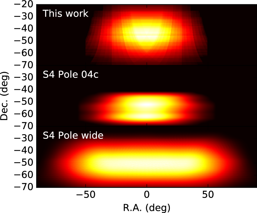
Figure 1.— Top: weight map for the scan trajectory and FP layout defined in this work. Middle: weight map for the deep Pole field (“experiment definition 04c”) from the CMB-S4 $r$-forecasting group. Bottom : weight map for the wide Pole field, centered in this plot on R.A. $=0^{\circ}$ to aid visual comparison, rather than R.A. $=30^{\circ}$ as it could be in reality to avoid galactic foregrounds.

2.4. TOD Simulation

As described in Section 2.2, the mock beams are defined on a regular Cartesian grid, $(x_{j},y_{j})$. We convert these to polar coordinates, $(r_{j},\phi_{j})$, which we define as offsets in spherical coordinates relative to the centroid when the beam is projected onto the sky. Given the trajectory of the $k$th detector’s centroid defined in Section 2.3, we compute the R.A. and Dec. trajectory of each pixel $j$ in the discretized beam. We then sample the simulated maps described in Section 2.1 along these trajectories using the get_interp_val routine of Healpy to form time streams $T_{k,j}(t)$, $Q_{k,j}(t)$ and $U_{k,j}(t)$. Multiplying each time stream by the value of the beam and summing yields the beam convolved $T$, $Q$, and $U$ trajectories for detector $k$,

$$T_{k}(t)=\sum_{j}B_{k}(r_{j},\phi_{j})T_{k,j}(t),$$ (5)

and similarly for $Q_{k}(t)$ and $U_{k}(t)$. The observed TOD for the $k$th detector is then computed as

$$s_{k}(t)=T_{k}(t)+Q_{k}(t)\cos[2\chi_{k}(t)]+U_{k}(t)\sin[2\chi_{k}(t)]$$ (6)

where $\chi_{k}(t)$ is the polarization angle of the detector as a function of time. We then compute the pair-difference time stream of the $i$th pair by differencing the A and B detector time streams within a pair,

$$d_{i}(t)=[s_{k=2i}(t)-s_{k=2i+1}(t)]/2.$$ (7)

We produce noiseless $\Lambda$CDM as well as $E$-only simulations by sampling off the maps described in Section 2.1. We also produce “leakage” sims by setting $Q_{k}(t)=U_{k}(t)=0$, so that the only non-zero component of $d_{i}(t)$ must be due to T$\rightarrow$P leakage from beam mismatch (i.e. $B_{2i}\neq B_{2i+1}$).

Lastly, we produce noise simulations by replacing the TOD with random Gaussian numbers of mean zero and a width tuned to produce next-generation survey noise levels after coadding over detectors.

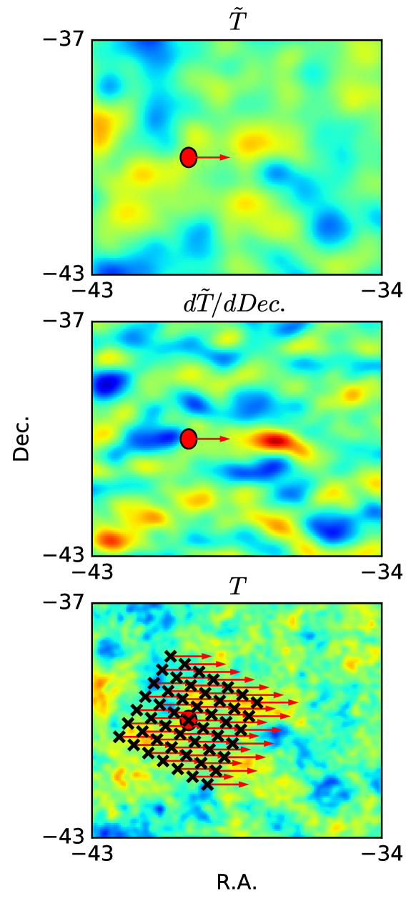
Figure 2.— Illustration of the construction of elliptical Gaussian leakage templates (top and middle) and arbitrary leakage templates (bottom). The top panel shows the nominal-beam-smoothed CMB temperature map, $\tilde{T}$, used to construct the differential gain template. The red circle illustrates a single detector-pair. The red arrow illustrates a short section of the trajectory of the detector-pair centroid during a typical fixed-elevation scan at the South Pole. The middle panel shows the smoothed first derivative map used to construct the differential pointing leakage template. The bottom panel shows the unsmoothed $T$ map and the grid defining the $N$ arbitrary leakage template trajectories. (The grid point spacing has been increased from $0.1^{\circ}$ to $0.4^{\circ}$ for visual clarity.) The rotation of the grid about the beam centroid is for one of the 8 boresight angles.

3. Mapmaking and Deprojection

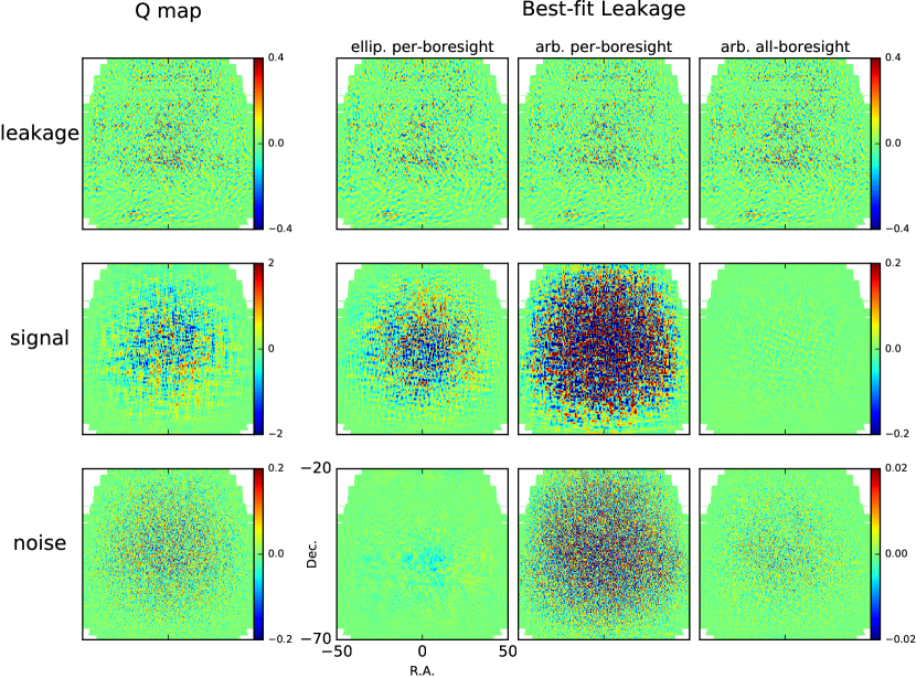
Figure 3.— Simulated $Q$ maps and best-fit leakage templates, broken down into simulation components and apodized by the weight map in the top panel of Figure 1. (N.B., the aspect ratio of the maps in this plot is not faithful.) Rows from top to bottom show the three simulation components: T$\rightarrow$P leakage, $\Lambda$CDM + dust signal, and instrumental noise. The leftmost column shows the simulated $Q$ map, coadded over all detectors and boresight angles, prior to deprojection. The remaining three columns show the best-fit leakage templates for different deprojection options. The “ellip. per-boresight” column shows the template for elliptical Gaussian deprojection in which leakage templates are fit to data from each boresight angle separately. The “arb. per-boresight” column shows the arbitrary deprojection best-fit template, also fitting to each boresight angle separately. The “arb. all-boresight” column shows the arbitrary deprojection template when fitting all boresight angles simultaneously. The $Q$ maps on the left would be deprojected by subtracting one of the corresponding three maps on the right.

We then bin the TODs into maps. We also construct time-ordered templates of T$\rightarrow$P leakage and bin each of these into maps as well. We fit the these binned leakage templates to the data and subtract them to deproject contamination from beam shape mismatch. Overfitting will also filter some “true” signal. The goal is to minimize this by keeping the complexity of the model to a minimum.

3.1. Mapmaking

We bin the simulated TODs into maps based on the procedure in Bicep2 Collaboration I (2014). Like the Bicep/Keck maps, the map pixel boundaries are defined as a grid in R.A. and Dec. with size $0.25^{\circ}$ in Dec. and size in R.A. chosen to make the pixels square along the central row.

For each pair $i$, we bin into map pixels various products of: (1) the pair difference TOD, $d_{i}(t)$; (2) the instantaneous weight, $w_{i}(t)$, which here we set to 1 for all time samples for all pairs; and (3) $\sin 2\chi_{i}$ and $\cos 2\chi_{i}$, where $\chi$ is the A detector’s polarization angle projected onto the sky. We bin those products needed to later reconstruct $Q$ and $U$. The binned quantity for each detector pair is referred to as a “pair-map” and is denoted

$$m_{i}(\alpha_{p},\delta_{p})=\sum_{l}q_{i}(t_{l}),$$ (8)

where the sum is over time samples for which the $i$th detector-pair’s centroid lies within the boundaries of pixel $p$ (which is centered on R.A. $\alpha_{p}$ and Dec. $\delta_{p}$), and

$$q_{i} \subset [w_{i},w_{i}d_{i},w_{i}d_{i}\cos 2\chi_{i},w_{i}d_{i}\sin 2\chi_{i},$$

$$\cos^{2}2\chi_{i},\sin^{2}2\chi_{i},\cos 2\chi_{i}\sin 2\chi_{i}].$$

This set of $q_{i}$ are the minimum quantities needed to later solve for $Q$, and $U$. They also have the property that they may be coadded over time, over detectors, and over polarization angles. Technically, the quantity $w_{i}d_{i}$ is not needed to construct the $Q$ and $U$ maps, but we later fit systematics templates to it. We bin data from different boresight angles separately so that there is a separate pair-map for each angle. The final step is to coadd over boresight angles and solve for $Q$ and $U$, the mathematical details of which we do not give here.

3.2. Leakage template construction

We also generate templates of T$\rightarrow$P leakage. In general, we model the T$\rightarrow$P leakage in $d_{i}(t)$ as the linear combination of $N$ “leakage templates”, $l_{i,n}$, so that the total contamination is

$$L_{i}(t)=\sum_{n=1}^{N}a_{i,n}l_{i,n}(t).$$ (10)

Leakage templates are simultaneously fit to the data at either the time-ordered level or the pair-map level to determine the $a_{i,n}$. BKIII fits leakage templates directly to $d_{i}(t)$ on timescales that include contiguous observations from a single boresight angle. This has the benefit of removing any leakage that varies on timescales longer than this. There is good reason to expect, however, that the beam is constant in time over a season, and indeed there is no evidence for temporal or boresight angle beam dependence in Bicep/Keck science or calibration data. We therefore opt to first coadd the data into pair-maps without first deprojecting, and fit the similarly coadded leakage templates in map-space. We coadd each time-ordered leakage template by binning it into map pixels like the data,

$$m_{i,n}^{T\rightarrow P}(\alpha_{p},\delta_{p})=\sum_{l}q_{i,n}(t_{l}),$$ (11)

with

$$q_{i,n}\subset[w_{i}l_{i,n},w_{i}l_{i,n}\cos 2\chi_{i},w_{i}l_{i,n}\sin 2\chi_{i}].$$ (12)

For each detector pair, we fit the $N$ binned $w_{i}l_{i,n}$ leakage templates to the $w_{i}d_{i}$ pair-map to find the $a_{i,n}$. We then multiply the $w_{i}l_{i,n}\sin 2\chi_{i}$ and $w_{i}l_{i,n}\cos 2\chi_{i}$ leakage templates by the best-fit $a_{i,n}$, sum over $n$, and store this single best-fit leakage pair-map for that detector pair. Lastly, we coadd the summed leakage templates over detector-pairs to construct the best-fit $Q$ and $U$ leakage templates, which we subtract from the maps.

Because we make a separate pair-map for each boresight angle, leakage does not cancel in the maps prior to fitting. As noted, deprojecting in pairmap-space will not perfectly remove mismatch that varies with time, as might be expected from detector gain mismatch. We therefore envision that differential gain deprojection will first be done at the time stream level, as is currently done by Bicep/Keck.

We alternately deproject two kinds of leakage templates: elliptical Gaussian leakage templates like those described in BKIII, which model the beams as elliptical Gaussians, and “arbitrary” leakage templates, which make no assumptions about the beam shape. BKIII simultaneously fits the ($N=6$) $l_{i,n}$ corresponding to the modes of a mismatched elliptical Gaussian directly to $d_{i}$. We form the same $l_{i,n}$ as in BKIII. Briefly summarized, we construct them by first smoothing the (simulated) Planck $T$ map to the nominal beam, a circular Gaussian of width FWHM$=0.5^{\circ}$. We then sample this map along with its first and second derivatives along the detector-pair’s trajectory. We then form the linear combinations of these derivative map time streams that approximate the leakage from the modes of mismatched elliptical Gaussians. There is one mode for amplitude mismatch (i.e. differential gain), two for centroid (differential pointing), one for beam width, and two for ellipticity. Although we bin these leakage templates into pair-maps prior to fitting to data (unlike BKIII which fits in the time domain), we still fit data from each boresight angle separately. Thus, while the total number of data points being fit is greatly reduced relative to BKIII, the fractional degrees of freedom being removed from the map is comparable. Another difference with the implementation of deprojection by Bicep/Keck is that we fit for the differential ellipticity coefficients. The Bicep/Keck results all set these coefficients to values determined from external calibration data. The reason for this is that fitting for these coefficients strongly filters the $TE$ spectrum and somewhat filters the $EE$ spectrum, a phenomenon arising from the inherent correlation between the $T$-map-derived leakage templates and the underlying $\Lambda$CDM $E$-mode signal.

In addition to the elliptical Gaussian templates, we also form deprojection templates that make no assumption about beam shape. At each time sample in the TOD, we form a gnomonic projection of the unsmoothed simulated Planck $T$ map centered on the detector-pair centroid. We define the projection grid with respect to FP coordinates $\{x,y\}$ so that the projection rotates with the projected orientation of the FP on the sky. The time series for a given grid point is the leakage template, $l_{i,n}(t)$. The projection size is $2.4^{\circ}\times 2.4^{\circ}$ with a grid spacing of $0.1^{\circ}$, so that the number of grid points is $N=576$. When fitting the binned arbitrary leakage templates to the data, we alternately fit data from each boresight angle separately to allow direct comparison with differential ellipticity deprojection, and fit all boresight angles simultaneously to reduce the filtering of the true signal.

Figure 2 illustrates the difference between the elliptical Gaussian and arbitrary leakage templates. The top two panels illustrate differential ellipticity template construction, showing a single detector-pair’s trajectory along the SAT-beam-smoothed $T$ map and one of its derivatives. (The map is zoomed in for clarity, and the other derivative maps are omitted for space.) The pair’s differential gain leakage template is constructed by sampling the smoothed $T$ map along this trajectory. The leakage template for the North-South component of differential pointing would be constructed by sampling the first derivative map off the same trajectory. The bottom panel illustrates arbitrary template construction, with multiple trajectories along the single unsmoothed $T$ map. The grid shown in Figure 2 is the same size as used in this work ($2.4^{\circ}\times 2.4^{\circ}$) but the spacing shown is $0.4^{\circ}$ instead of $0.1^{\circ}$ for clarity. In principle, the $a_{i,n}$ for the arbitrary templates can be chosen to construct the smoothed first derivative map, as well as any other derivatives, or linear combinations thereof.

4. Results

Lastly, we deproject the simulated T$\rightarrow$P leakage. We show the results in maps and in their angular power spectra.

4.1. Results in map space

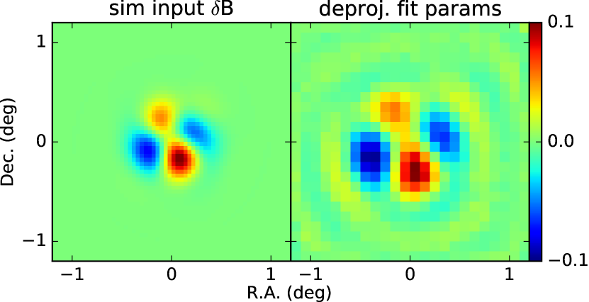
Figure 4.— Left: the simulated difference beam for a single peak normalized detector pair. Right: best-fit arbitrary deprojection coefficients for this detector pair in a single realization of the leakage-only simulations.

The $Q$ map for a single realization, broken down by simulation input component, and the corresponding best-fit leakage templates under different deprojection schemes are shown in Figure 3. Each row is one of the three components of the simulation: T$\rightarrow$P leakage, $\Lambda$CDM + dust signal, and noise. The left column shows the simulated maps “as observed” by our mock survey. The other columns show the best-fit leakage templates for different deprojection options. Maps and leakage templates are coadded over all boresight angles and detectors.

The top row shows the T$\rightarrow$P leakage component. Because the simulated beams described in Section 2.2 were intentionally constructed to be close to (but not quite) elliptical Gaussians, the best-fit templates are nearly indistinguishable both from each other and from the actual leakage. As will be shown later, however, the residuals are much lower for the arbitrary templates.

The middle and bottom rows shows the signal and noise components, respectively. Any non-zero values in these best-fit leakage templates are due to overfitting and result in filtering of the true signal when subtracted from the maps. The elliptical Gaussian template, shown in the second column, establishes a baseline level of overfitting that is de facto acceptable for Stage-III and Stage-IV experiments. This is because elliptical Gaussian deprojection is used by Bicep/Keck for all its $r$-constraints, and because the CMB-S4 inflation projections use the achieved Bicep/Keck $BB$ noise levels as the starting point for scaling to Stage-IV detector counts (CMB-S4 Collaboration, 2019). Any reduction of S/N caused by preferentially filtering signal is already built into these projections. It should be noted that elliptical Gaussian deprojection as actually implemented by Bicep/Keck (and therefore baselined by CMB-S4) is slightly different than what is implemented here. Bicep/Keck fits for only 4 of the 6 differential beam parameters; the differential ellipticity coefficients are fixed to values measured from beam maps. This slightly reduces the amount of overfitting in the Bicep/Keck analysis is therefore not perfectly comparable to our implementation of elliptical Gaussian deprojection, which fits for all parameters. Nonetheless, Barkats et al. (2014) demonstrates that filtering from differential gain deprojection is negligible compared to azimuth-fixed template subtraction, which suppresses power by $\sim 50\%$ in the lowest Bicep/Keck $EE$ bandpower. Since azimuth-fixed template subtraction is implicitly baselined in the CMB-S4 projections, it should be a safe assumption that demonstrating the absence of filtering in excess of elliptical Gaussian deprojection is sufficient to demonstrate the suitability of arbitrary deprojection for next-generation surveys.

Arbitrary deprojection on a per-boresight angle basis results in greater overfitting relative to elliptical Gaussian deprojection, as shown by the larger amplitude of the “arb. per-boresight angle” template relative to the “ellip. per-boresight angle” template in the middle and bottom rows. This is unsurprising given that the number of templates being fit is 576 vs. 6.

When fitting the arbitrary templates to all 8 boresight angles simultaneously, however, as shown in the the “arb. all-boresight angle” column, the overfitting of the signal component is less than with ellipticity deprojection. The overfitting of the noise component is somewhat higher at small scales, though in fact is comparable at degree scales. This result is perhaps surprising because, even though the number of map pixels being fit is $\approx 8\times$ greater relative to elliptical Gaussian deprojection, the number of templates being fit is $\approx 100\times$ greater. The naive expectation would be that more degrees of freedom would be removed from the map. We interpret this result as a consequence of correlations between the arbitrary leakage templates. Generally treated as a potential problem in regression, the reduction of effective degrees of freedom in the leakage model of Equation 10 works in our favor. In fact, since the correlation length of the CMB is $\sim 1^{\circ}$, then there are $\sim 6$ independent modes in our $2.4^{\circ}\times 2.4^{\circ}$ grid of leakage templates, regardless of grid spacing.

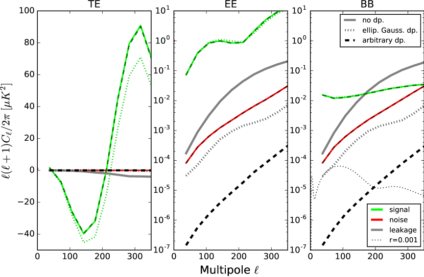
Figure 5.— Angular power spectra of the simulated maps before and after deprojection. The green, red, and gray lines show the signal, noise, and T$\rightarrow$P leakage components, respectively. The solid, dotted, and dashed lines show the spectra before deprojection, after elliptical Gaussian deprojection, and after all-boresight arbitrary deprojection, respectively.

Figure 4 shows the simulated difference beam for a single detector-pair along with the best-fit $a_{n}$ from the leakage-only simulation. The fit coefficients are normalized to have the same peak value as the input difference beam. The two show good qualitative agreement, but there is an apparent rescaling of the best-fit beam. We suspect that this is the combined effect of Planck noise and correlations among templates. Intuitively, there is a degeneracy between the angular separation of features in the best-fit beam and their amplitude. For instance, differential pointing manifests as a dipolar difference beam, which couples to the first derivative of the $T$ map. To third order, a perturbation to the centroid offset within a detector-pair can be approximated by either an increase in the dipole separation or an increase in its amplitude. While it is possible to construct a forward simulation, mapmaking, and deprojection pipeline in which the known differential beam is exactly recovered, we purposefully do not perform our forward simulation in exactly same way as the template generation. We also include the effect of Planck $T$ map noise in the template. We therefore do not necessarily expect perfect agreement between the recovered fit coefficients and the input beam.

In principle, multicollinearity among regressors can lead to biased predictions of the leakage if the coefficients derived from a regression on one data set are used to generate predictions of leakage in a disjoint data set. Deprojection both fits and predicts leakage using the same data so this is not an issue for the current work. Furthermore, to the extent it could be an issue, our simulations include it. What would perhaps be a problem is if coefficients determined from fits to data whose dominant signal has a different scale length than the CMB (like, say, galactic foregrounds) were used to predict leakage in a CMB-dominated field. In this case, our method might yield a biased prediction and would need to be tested on simulations.

4.2. Results in Angular Power Spectra

Lastly, we subtract the best-fit leakage templates from the maps and compute the resulting angular power spectra. We again do so for the three simulated components separately. Angular power spectra are calculated as in Bicep2 Collaboration I (2014). Briefly, we multiply the maps by the weight map, zero pad, compute the 2D power spectrum with an FFT, and bin into 1D bandpowers. We account for E$\rightarrow$B mixing by computing the $B$-mode 2D Fourier plane of the $E$-only sims and subtracting these modes directly in the Fourier plane of the $\Lambda$CDM + dust sims. This, of course, is not an option in reality since one can not know the pure-E component ahead of time. “Pure-B” estimators that do not leak E$\rightarrow$B for filtered maps are used to avoid this (Bicep2 and Keck Array Collaborations VII, 2016), but we have not implemented one, and so use this simulation-friendly workaround. Lastly, we correct the bandpowers for beam suppression by a circular Gaussian using the appropriate analytic beam window function.

Figure 5 shows the angular power spectra of the coadded maps prior to deprojection, after ellipticity deprojection, and after all-boresight-angle arbitrary deprojection. We unsurprisingly find that arbitrary beam deprojection removes almost all of the leakage while elliptical Gaussian deprojection leaves a significant undeprojected residual. The size of this residual is, of course, dependent on the component of the simulated beams that is not modeled by an elliptical Gaussian, something we are free to choose in our simulations. We chose the beams so that the residual with elliptical Gaussian deprojection would be small but important for next-generation CMB surveys, which report projected sensitivities in the neighborhood of $\sigma_{r}=5\times 10^{-4}$. The undeprojected residual with arbitrary deprojection is of the order $r\approx 1\times 10^{-5}$, more than sufficient for the future.

The filtering of all true signal appears negligible. Happily, arbitrary deprojection does not appreciably filter $EE$ and $TE$ like ellipticity deprojection does. We therefore conclude that our method is a success.

5. Conclusions

We conclude that arbitrary deprojection, performed over all boresight angles simultaneously, solves the problem of T$\rightarrow$P leakage from main beam mismatch for next-generation CMB surveys. Our templates extend out to a distance of $1.2^{\circ}$ from the beam centroids, so leakage arising from near and far sidelobes will not be cleaned by this procedure. Possibly, the templates can be extended to larger distances to encompass near sidelobes. Extending the templates to encompass far sidelobes will probably result in too much filtering of signal. It may be possible to construct a second set of coarsely gridded templates from smoothed $T$ maps to deproject sidelobe leakage under the assumption that sidelobes have smoother features than the main beam. Nonetheless, beam maps of sidelobes will almost certainly remain a crucial component of next-generation CMB surveys. Arbitrary deprojection of main beam leakage can allow more effort to be placed here.

References

- Bicep2 Collaboration III (2015) Bicep2 Collaboration III, Astrophys. J. 814, 110 (2015), arXiv:1502.00608 [astro-ph.IM] .
- Bicep2 and Keck Array Collaborations IV (2015) Bicep2 and Keck Array Collaborations IV, Astrophys. J. 806, 206 (2015), arXiv:1502.00596 [astro-ph.IM] .
- Bicep2 and Keck Array Collaborations XI (2019) Bicep2 and Keck Array Collaborations XI, Astrophys. J. 884, 114 (2019), arXiv:1904.01640 [astro-ph.IM] .
- Planck Collaboration et al. (2014) Planck Collaboration, P. A. R. Ade, N. Aghanim, C. Armitage-Caplan, M. Arnaud, M. Ashdown, F. Atrio-Barandela, J. Aumont, C. Baccigalupi, A. J. Banday, and et al., Astr. & Astroph. 571, A16 (2014), arXiv:1303.5076 .
- Zaldarriaga and Seljak (1998) M. Zaldarriaga and U. Seljak, Phys. Rev. D 58, 023003 (1998), astro-ph/9803150 .
- Planck Collaboration et al. (2016a) Planck Collaboration, R. Adam, P. A. R. Ade, N. Aghanim, M. Arnaud, J. Aumont, C. Baccigalupi, A. J. Banday, R. B. Barreiro, J. G. Bartlett, and et al., Astr. & Astroph. 586, A133 (2016a), arXiv:1409.5738 .
- Sheehy and Slosar (2018) C. Sheehy and A. Slosar, Phys. Rev. D 97, 043522 (2018), arXiv:1709.09729 .
- Bicep2 and Keck Array Collaborations X (2018) Bicep2 and Keck Array Collaborations X, Physical Review Letters 121, 221301 (2018), arXiv:1810.05216 .
- Planck Collaboration et al. (2016b) Planck Collaboration, P. A. R. Ade, N. Aghanim, M. Arnaud, M. Ashdown, J. Aumont, C. Baccigalupi, A. J. Banday, R. B. Barreiro, J. G. Bartlett, and et al., Astr. & Astroph. 594, A12 (2016b), arXiv:1509.06348 .
- Hui and BICEP Array Collaboration (2018) H. Hui and BICEP Array Collaboration, in Proc. SPIE, Society of Photo-Optical Instrumentation Engineers (SPIE) Conference Series, Vol. 10708 (2018) p. 1070807, arXiv:1808.00568 [astro-ph.IM] .
- Crumrine and BICEP Array Collaboration (2018) M. Crumrine and BICEP Array Collaboration, in Proc. SPIE, Society of Photo-Optical Instrumentation Engineers (SPIE) Conference Series, Vol. 10708 (2018) p. 107082D, arXiv:1808.00569 [astro-ph.IM] .
- CMB-S4 Collaboration (2019) CMB-S4 Collaboration, arXiv e-prints , arXiv:1907.04473 (2019), arXiv:1907.04473 [astro-ph.IM] .
- Bicep2 Collaboration I (2014) Bicep2 Collaboration I, Physical Review Letters 112, 241101 (2014), arXiv:1403.3985 .
- Barkats et al. (2014) D. Barkats, R. Aikin, C. Bischoff, I. Buder, J. P. Kaufman, B. G. Keating, J. M. Kovac, M. Su, P. A. R. Ade, J. O. Battle, E. M. Bierman, J. J. Bock, H. C. Chiang, C. D. Dowell, L. Duband, J. Filippini, E. F. Hivon, W. L. Holzapfel, V. V. Hristov, W. C. Jones, C. L. Kuo, E. M. Leitch, P. V. Mason, T. Matsumura, H. T. Nguyen, N. Ponthieu, C. Pryke, S. Richter, G. Rocha, C. Sheehy, S. S. Kernasovskiy, Y. D. Takahashi, J. E. Tolan, and K. W. Yoon, Astrophys. J. 783, 67 (2014), arXiv:1310.1422 .
- Bicep2 and Keck Array Collaborations VII (2016) Bicep2 and Keck Array Collaborations VII, Astrophys. J. 825, 66 (2016), arXiv:1603.05976 [astro-ph.IM] .