Phase-separation of vector solitons in spin-orbit coupled spin-$1$ condensates

Abstract

We study the phase-separation in three-component bright vector solitons in a quasi-one-dimensional spin-orbit-coupled hyper-fine spin $F=1$ ferromagnetic Bose-Einstein condensate upon an increase of the strength of spin-orbit (SO) coupling $p_{x}\Sigma_{z}$ above a critical value, where $p_{x}$ is the linear momentum and $\Sigma_{z}$ is the $z$-component of the spin-1 matrix. The bright vector solitons are demonstrated to be mobile and dynamically stable. The collision between two such vector solitons is found to be elastic at all velocities with the conservation of density of each vector soliton. The two colliding vector solitons repel at small separation and at very small colliding velocity, they come close and bounce back with the same velocity without ever encountering each other. This repulsion produced by SO coupling is responsible for the phase separation in a vector soliton for large strengths of SO coupling. The collision dynamics is found to be completely insensitive to the relative phase of the colliding solitons. However, in the absence of SO coupling, at very small velocity, the two colliding vector solitons attract each other and form a vector soliton molecule and the collision dynamics is sensitive to the relative phase as in scalar solitons. The present investigation is carried out through a numerical solution and an analytic variational approximation of the underlying mean-field Gross-Pitaevskii equation.

I Introduction

Bright solitons are self-bound solitary wave that can move at a constant velocity maintaining its shape due to a cancellation of linear repulsion and non-linear attraction. Such solitons have been found Kivshar in water waves, non-linear optics, and Bose-Einstein condensates (BECs) among others. Bright solitons have been created in a BEC of ⁷Li li and ⁸⁵Rb rb atoms by a management of the non-linear attraction near a Feshbach resonance Inouye . Solitons have also been studied in binary BEC mixtures Perez-Garcia .

After the experimental observation of a spinor BEC of ²³Na atoms with hyper-fine spin $F=1$ exp , mean-field theory to study these have been developed Ohmi . Although there could not be any natural spin-orbit (SO) coupling in a spinor BEC of neutral atoms, an artificial synthetic SO coupling can be realized in a spinor BEC by a management of external electromagnetic fields stringari ; rev . Different managements are possible which lead to a different types of SO coupling between spin and momentum in the mean-field equation of a spinor BEC. Two such possible SO couplings are due to Rashba Rashba and Dresselhaus Dresselhaus and other types of SO coupling are possible. An equal mixture Rashba and Dresselhaus SO couplings was first realized experimentally in a pseudo spin-1/2 spinor BEC formed of two ($F_{z}=0$ and $-1$) of the three hyper-fine spin components of the $F=1$ state 5S_1/2 of ⁸⁷Rb Lin . After this pioneering experiment, similar SO-coupled BEC was formed and studied in different laboratories diff . Different possible SO couplings in spinor BECs and the ways to engineer these in a laboratory are addressed in review articles stringari . Possible ways of realizing the SO coupling in three-component spin-1 BEC have been discussed SOspin1 . The three components ($F_{z}=\pm 1,0$) corresponding to three spin projections of the spin-1 operator $\Sigma$ will be denoted by the subscripts $\pm 1$ and 0.

Solitons have been extensively studied in spinor BECs without SO coupling Ieda . Novel phases SOspin1 and solitonic structures in SO-coupled pseudo-spin-$1/2$ rela and spin-$1$ Liu ; sol1d BECs have also been investigated theoretically. These studies were extended to quasi-solitons confined in two sol2d and three sol3d dimensions. Different types of SO coupling introduce rich dynamics through different types of derivative couplings among the component wave functions of the mean-field model.

A spin-$1$ spinor BEC is controlled by two interaction strengths, e.g., $c_{0}\propto(a_{0}+2a_{2})/3$ and $c_{2}\propto(a_{2}-a_{0})/3$, with $a_{0}$ and $a_{2}$ the scattering lengths in total spin $F=0$ and 2 channels, respectively Ohmi . All spin-1 spinor BECs can be classified into two distinct types Ohmi ; stringari : ferromagnetic ($c_{2}<0$) and anti-ferromagnetic ($c_{2}>0$). In this paper, we study three-component vector solitons in a SO-coupled spin-$1$ ferromagnetic BEC in a quasi-one-dimensional (quasi-1D) trap using a mean-field coupled Gross-Pitaevskii (GP) equation.

We consider a distinct SO coupling usedspin1/2 ; usedspin1/2x $(\propto\gamma p_{x}\Sigma_{z})$ where $p_{x}$ is the $x$ component of momentum, $\gamma$ the strength of SO coupling, and $\Sigma_{z}$ is the $z$ component of the spin-1 spin matrix. In a laboratory, this SO coupling can be obtained by two counter-propagating polarized laser fields of slightly different frequencies. A Raman coupling due to the lasers induces transitions between the three spin components of the spin-1 BEC, providing, at the same time, a momentum transfer along $x$ direction, which determines the strength $\gamma$ of SO coupling. As has been shown usedspin1/2 , this SO coupling appears in the single particle Hamiltonian by applying a unitary transformation to the Hamiltonian in the laboratory frame describing the system in the presence of detuned, spin-polarized laser fields. The unitary transformation consists of a local rotation in spin space around the $z$ axis. With this SO coupling, we identify novel three-component vector solitons in a quasi-1D BEC along the $x$ direction in the ferromagnetic domain. For small values of the strength $\gamma$ of SO coupling and also in its absence ($\gamma=0$), an overlapping three-component vector soliton is formed in a ferromagnetic BEC. With the increase of the strength $\gamma$ of SO coupling above a critical value $\gamma_{c}$, a phase separation takes place between the $F_{z}=\pm 1$ components and the third $F_{z}=0$ component vanishes, thus forming a completely phase separated two-component vector soliton. Actually, both types of these solitons $-$ two-component and three-component $-$ exist above and below the critical SO-coupling strength $\gamma=\gamma_{c}$. For $\gamma<\gamma_{c}$, the overlapping soliton is the minimum-energy ground state and the phase-separated soliton is an excited state; whereas, for $\gamma>\gamma_{c}$, the opposite is true. In a previous study with a different SO coupling $(\propto p_{x}\Sigma_{x})$ sol1d we found distinct types of solitons in the ferromagnetic and anti-ferromagnetic domains. The ferromagnetic solitons are true mobile overlapping solitons with single-peak structure. The anti-ferromagnetic solitons usually have multi-peak structure and could not move maintaining the shapes of the components. The present ferromagnetic solitons are true mobile solitons.

In the SO-coupled GP equation, we use a plausible analytic approximation and a variational scheme to determine the densities of the SO-coupled ferromagnetic bright solitons in the two above-mentioned domains $-$ overlapping and phase-separated $-$ minimizing the energy functional. The appropriate variational ansatz in each of the domains is constructed using a knowledge about the solutions of the SO-coupled equation. The variational analysis provides the necessary and sufficient conditions which the interaction strengths $c_{0}$ and $c_{2}$ must satisfy to obtain a stable bright soliton. In addition to the densities and energies of the soliton, the analytic variational method also yields the critical SO-coupling strength for a phase separation of the components of the vector soliton. We also compare all these analytic variational results with the numerical solution the GP equation obtained by imaginary-time propagation for the stationary vector solitons.

We study the dynamics of the vector soliton numerically by real-time simulation. The dynamical stability of the vector soliton was established. The phase separation of a three-component vector soliton was also demonstrated by real-time propagation upon changing the SO-coupling strength from a value below $\gamma_{c}$ to a value above it. We demonstrate that the present vector soliton can propagate maintaining its shape, although the SO-coupled GP equation is not Galilean invariant. The collision between two overlapping SO-coupled ferromagnetic vector solitons, quite different from three-component solitons without SO coupling, is found to be elastic at all velocities with the conservation of density. The two vector solitons repel at small distances, and at small colliding velocities, they come close and bounce back without ever encountering each other. Quite different from two scalar solitons, the collision dynamics of two SO-coupled vector solitons remain unchanged after a change of relative phase between the two SO-coupled vector solitons. To demonstrate that the two unusual properties of collision $-$ (i) elastic nature at all velocities and (ii) insensitivity to relative phase $-$ are caused by the SO coupling, we study the collision dynamics at small velocity of two vector solitons in the absence of SO coupling. In that case, after collision the two vector solitons attract and form a vector soliton molecule in an excited state which never separate. Also, the collision dynamics, with the SO coupling switched off, is found to be very sensitive to the relative phase between the two solitons as in scalar solitons

In Sec. II, we describe the mean-field model GP equation for a SO-coupled spin-$1$ spinor BEC. We provide analytic variational solution of this model for the overlapping vector soliton and for its phase-separated counterpart. In Sec. III, we provide a numerical solution of our model for the two types of solitons and compare the results for density and energy with the corresponding analytic variational results. We also study the dynamics of the vector soliton and the transition from an overlapping to phase-separated vector soliton with the increase of SO coupling. The collision dynamics of two overlapping vector soliton was also studied at different colliding velocities. In Sec. IV a summary of our findings is presented.

II Analytical Formulation

II.1 Mean-field model for a SO-coupled BEC

We consider a SO-coupled spinor BEC in a quasi-1D trap along the $x$ axis. This quasi-1D trap is realized by strong traps in $y$ and $z$ directions, so that the system is frozen in Gaussian ground states in these directions and the essential dynamics of the system is realized in the $x$ direction Salasnich . The single particle Hamiltonian of the condensate in this quasi-1D trap is taken in scaled dimensionless units $\hbar={\bar{\bf m}}=1$ as usedspin1/2

$$H_{0}=\frac{p_{x}^{2}}{2}+\gamma p_{x}\Sigma_{z},$$ (1)

where $\bar{\bf m}$ is the mass of an atom, $p_{x}=-i\partial/\partial x$ is the momentum operator along $x$ axis, and $\Sigma_{z}$ is the irreducible representation of the $z$ component of the spin-1 spin matrix:

$$\Sigma_{z}=\left(\begin{array}[]{ccccc}1&0&0\\ 0&0&0\\ 0&0&-1\end{array}\right),$$ (5)

As we will be investigating vector solitons in this paper we will not include any trapping potential in the Hamiltonian. This SO-coupling is distinct from a previous SO coupling gautam-1 ; gautam-2 $(\gamma p_{x}\Sigma_{x})$ used in the study of a quasi-1D BEC.

Using the single particle model Hamiltonian (1) and considering interactions in the Hartree approximation, a quasi-1D Salasnich spin-1 BEC can be described by the following set of three coupled mean-field partial differential GP equations for the wave-function components $\phi_{j}$ Ohmi

$$i\frac{\partial\phi_{\pm 1}}{\partial{t}} =\left(-\frac{1}{2}\frac{\partial^{2}}{\partial{x}^{2}}+{c}_{0}{\rho}\right)\phi_{\pm 1}\mp{i{\gamma}}\frac{\partial\phi_{\pm 1}}{\partial x}$$

$$+c_{2}({\rho}_{\pm 1}+{\rho}_{0}-{\rho}_{\mp 1})\phi_{\pm 1}+c_{2}\phi_{0}^{2}\phi_{\mp 1}^{*},$$ (6)

$$i\frac{\partial\phi_{0}}{\partial{t}} =\left(-\frac{1}{2}\frac{\partial^{2}}{\partial{x}^{2}}+{c}_{0}{\rho}\right)\phi_{0}$$

$$+c_{2}({\rho}_{+1}+{\rho}_{-1})\phi_{0}+2{c}_{2}\phi_{0}^{*}\phi_{+1}\phi_{-1},$$ (7)

where interaction strengths abc2 ${c}_{0}=2N(a_{0}+2a_{2})l_{0}/3l_{yz}^{2}$, ${c}_{2}=2N(a_{2}-a_{2})l_{0}/3l_{yz}^{2}$, component density ${\rho}_{j}=|\phi_{j}|^{2}$ with $j=+1,0,-1$ corresponding to the three components of the spin-1 spinor $F_{z}=+1,0,-1$, and total density ${\rho}=(\rho_{+1}+\rho_{0}+\rho_{-1})$, $l_{yz}$ is the harmonic oscillator length in the transverse $yz$ directions and $l_{0}$, in the absense of a trap in $x$ direction, is a scaling length in $x$ direction. The densities are measured in units of $l^{-1}$. For notational simplicity, in Eqs. (6) and (7) we have not explicitly shown the space and time dependence of the wave function $\phi_{\pm 1,0}(x,t)$. The total density is normalized to unity, i.e., $\int_{-\infty}^{\infty}{\rho}({x})d{x}=1.$ The conserved magnetization is defined as $\int dx(\rho_{+1}-\rho_{-1})=m.$

II.2 Variational Approximation

The energy functional corresponding to the mean-field SO-coupled spinor BEC model (6) and (7) is Ohmi

$$E(\gamma) =\int_{-\infty}^{\infty}dx\Bigg{\{}\frac{1}{2}\left|\frac{d\phi_{+1}}{dx}\right|^{2}+\frac{1}{2}\left|\frac{d\phi_{0}}{dx}\right|^{2}+\frac{1}{2}\left|\frac{d\phi_{-1}}{dx}\right|^{2}+\frac{c_{0}}{2}\rho^{2}$$

$$+\frac{c_{2}}{2}\Big{[}\left(\rho_{+1}+\rho_{0}-\rho_{-1}\right)\rho_{+1}+\left(\rho_{0}+\rho_{-1}-\rho_{+1}\right)\rho_{-1}$$

$$+\left(\rho_{+1}+\rho_{-1}\right)\rho_{0}+2\left(\phi_{-1}^{*}\phi_{0}^{2}\phi_{+1}^{*}\right.\left.+\phi_{-1}\phi_{0}^{*2}\phi_{+1}\right)\Big{]}$$

$$+\gamma\left(-i\phi_{+1}^{*}\frac{d\phi_{+1}}{dx}+i\phi_{-1}^{*}\frac{d\phi_{-1}}{dx}\right)\Bigg{\}}.$$ (8)

We will minimize this energy functional using an analytic variational wave function to find the analytic solution of the SO-coupled GP equation. The analytic ansatz for the wave function is taken as

$$\Phi\equiv\left(\begin{array}[]{c}\phi_{+1}\\ \phi_{0}\\ \phi_{-1}\end{array}\right)=\frac{1}{2}\left(\begin{array}[]{c}e^{-i\gamma x}(1+m)\phi(x)\\ \sqrt{2(1-m^{2})}\phi(x)\\ e^{i\gamma x}(1-m)\phi(x)\end{array}\right),\quad\\$$ (9)

where $\phi(x)$ is taken to be a normalized Gaussian

$$\phi(x)=\left(\frac{1}{\pi\alpha^{2}}\right)^{1/4}\exp\left[-\frac{x^{2}}{2\alpha^{2}}\right],$$ (10)

or a hyperbolic secant function

$$\phi(x)=\frac{\sqrt{\sigma}}{\sqrt{2}}\mbox{sech}(\sigma x),$$ (11)

where the parameters $\alpha$ and $\sigma$ denote amplitude and width. In the case $\gamma=m=0$, the three components $\phi_{\pm 1},\phi_{0}$ are multiples of one another while ansatz (9) becomes an exact relation and the hyperbolic secant function (11) becomes an exact solution of Eqs. (6) and (7). With these ansatz for the wave function, the energy functional (II.2) is explicitly real, has the correct $\gamma$ dependence, and correct magnetization and normalization. The same functional form of the wave function components is consistent with the numerical solution of the GP model and was employed before to predict the component densities of trapped spin-1 and spin-2 spinor BECs in the form of single mode abc and decoupled-mode abc2 approximations. Here we are applying similar ideas to study the properties of a vector soliton.

With the Gaussian ansatz (10) for the profile of the vector soliton, the energy functional (II.2) becomes

$$E(\gamma)=-\frac{\gamma^{2}}{4}+\frac{1}{4\alpha^{2}}+\frac{c_{0}+c_{2}}{2\alpha\sqrt{2\pi}}.$$ (12)

This energy functional is independent of magnetization $m$. The width $\alpha$ of the minimum-energy ground state vector soliton is obtained by minimizing this energy functional with respect to $\alpha$:

$$\alpha=-\frac{\sqrt{2\pi}}{c_{0}+c_{2}}.$$ (13)

For this width to be positive we require $c_{0}+c_{2}<0$ in addition to $c_{2}<0$ (ferromagnetic). This width is independent of the SO-coupling strength $\gamma$ and also of magnetization $m$. The following minimum of energy as a function of $\gamma$ is obtained by substituting Eq. (13) in Eq. (12)

$$E(\gamma)=-\frac{\gamma^{2}}{4}-\frac{(c_{0}+c_{2})^{2}}{8\pi}\approx-\frac{\gamma^{2}}{4}-0.0397887(c_{0}+c_{2})^{2},$$ (14)

which is the energy of the minimum-energy spin-1 three-component vector soliton in the ground state. For the hyperbolic secant ansatz (11) for the wave function, energy functional (II.2) becomes

$$E(\gamma)=-\frac{\gamma^{2}}{4}+\frac{\sigma^{2}}{6}+\frac{(c_{0}+c_{2})\sigma}{6}.$$ (15)

The minimum of this energy occurs at

$$\sigma=-\frac{1}{2}(c_{0}+c_{2}),$$ (16)

provided $c_{0}+c_{2}<0.$ The minimum of energy (15) is

$$E(\gamma)=-\frac{\gamma^{2}}{4}-\frac{(c_{0}+c_{2})^{2}}{24}\approx-\frac{\gamma^{2}}{4}-0.0416667(c_{0}+c_{2})^{2}.$$ (17)

The energy (17) obtained with the hyperbolic secant ansatz (11) is smaller than energy (14) obtained with the Gaussian ansatz (10). Hence, because of the variational nature of the analytic approximation, the hyperbolic secant ansatz should give a better approximation, as will be verified in the numerical calculations in Sec. III.

We note that the analytic variational results (13) and (14), as well as (16) and (17), are determined by the net attraction $c_{0}+c_{2}$ and independent of the individual interaction strengths $c_{0}$ and $c_{2}$. The numerical results depend in a nontrivial way on the individual strengths $c_{0}$ and $c_{2}$, although we will see that in the weak-coupling limit of small nonlinear interaction the numerical results follow the analytic ones being determined by the net attraction. The effective nonlinear interaction in the GP equations (6) and (7) is $\sim|(c_{0}+c_{2})|\rho_{j,\mbox{av}}$, where $\rho_{j,\mbox{av}}$ is the average density of component $j$. This condition of weak coupling is valid for the numerical results presented in Sec. III.

Our numerical calculation revealed that for SO-coupling strength $\gamma$ larger than a critical value $\gamma_{c}$, a complete phase separation occurs between the $F_{z}=\pm 1$ components while the $F_{z}=0$ component vanishes. For $\gamma<\gamma_{c}$ the fully-overlapping three-component vector soliton is the lowest-energy soliton and for $\gamma>\gamma_{c}$ the fully-separated two-component vector soliton is the ground state. We could not find a partially separated vector soliton with non-zero $F_{z}=0$ component for any values of the parameters: $c_{0},c_{2}$ and $\gamma$. To study this crossover from three- to two-component ground state soliton analytically we note that if we set $\phi_{0}=\rho_{0}=0$, for vanishing $F_{z}=0$ component, and the overlap $\rho_{+1}\rho_{-1}=0$, for a complete phase separation, in Eqs. (6) and (7), then we get the following set of decoupled equations for the phase-separated two-component vector soliton

$$i\frac{\partial\phi_{\pm 1}}{\partial{t}}=\left[-\frac{1}{2}\frac{\partial^{2}}{\partial{x}^{2}}+\kappa_{\pm 1}{(c_{0}+c_{2})}\rho_{\pm 1}\mp{i{\gamma}}\frac{\partial}{\partial x}\right]\phi_{\pm 1},$$ (18)

where $\rho_{\pm 1}=|\phi_{\pm 1}|^{2}$, $\kappa_{\pm 1}=(1\pm m)/2$. As the coupling between the two components has been removed, the nonlinearities $\kappa_{\pm 1}(c_{0}+c_{2})$ are appropriate for magnetization $m$. Equation (18) has the following analytic solution

$$\phi_{\pm 1}\equiv\sqrt{{\kappa_{\pm 1}}}\widehat{\phi}_{\pm 1}=\sqrt{{\kappa_{\pm 1}}}e^{\mp i\gamma x}\sqrt{\frac{\sigma_{\pm 1}}{2}}\mathrm{sech}(\sigma_{\pm 1}x),$$ (19)

satisfying the condition of normalization and magnetization, e.g. $\int dx(\rho_{+1}+\rho_{-1})=1$ and $\int dx(\rho_{+1}-\rho_{-1})=m$, respectively, where $\sigma_{\pm 1}=\kappa_{\pm 1}(c_{0}+c_{2})/2$. The analytic solutions (19) of the decoupled equations (18) cannot, however, determine the position of individual solitons, which will be fixed in an ad-hoc fashion. The energy functional of Eq. (18) can now be written as

$$E(\gamma) =\sum_{j=\pm 1}\int\kappa_{j}\Biggr{[}\frac{1}{2}\left|\frac{d\widehat{\phi}_{j}}{dx}\right|^{2}+\frac{(c_{0}+c_{2})\kappa_{j}|\widehat{\phi}_{j}|^{4}}{2}$$

$$-i\gamma\widehat{\phi}_{j}^{*}\frac{d\widehat{\phi}_{j}}{dx}\Biggr{]}dx.$$ (20)

For zero magnetization $(m=0)$, using Eq. (19), energy (20) can be evaluated to yield

$$E(\gamma)=-\frac{\gamma^{2}}{2}-\frac{(c_{0}+c_{2})^{2}}{96}\approx-\frac{\gamma^{2}}{2}-0.0104167(c_{0}+c_{2})^{2}.$$ (21)

For small values of $\gamma$ ($\gamma<\gamma_{c}$), the energy of the two-component soliton (21) is greater than the energy of the three-component soliton (17), thus making the three-component vector soliton the ground state. The opposite happens for $\gamma>\gamma_{c}$, when the phase-separated two-component vector soliton becomes the ground state. The crossover takes place when the two minima of energy given by Eqs. (17) and (21) are equal, e.g., at

$$\gamma_{c}=-{\frac{1}{\sqrt{8}}}(c_{0}+c_{2})\approx-0.353553(c_{0}+c_{2}),$$ (22)

For $\gamma<\gamma_{c}$, $E(\gamma)$ of Eq. (17) is smaller than that of Eq. (21) making the overlapping state the ground state, as will be verified in our numerical calculation. As $\gamma$ increases past $\gamma_{c}$, for $\gamma>\gamma_{c}$ the opposite is true making the phase-separated state the ground state.

We now show that the phase separation of the vector soliton demonstrated above is a consequence of the SO coupling $\gamma p_{x}\Sigma_{z}$ used and it is not a general phenomenon common to other types of the SO coupling. This SO coupling is obtained by aligning the electromagnetic fields appropriately usedspin1/2 . In one dimension, for a spin-1 spinor, there are two other linearly independent SO couplings: $\gamma p_{x}\Sigma_{x}$ and $\gamma p_{x}\Sigma_{y}$, where

$$\Sigma_{x}=\frac{1}{\sqrt{2}}\left(\begin{array}[]{ccccc}0&1&0\\ 1&0&1\\ 0&1&0\end{array}\right),\Sigma_{y}=\frac{i}{\sqrt{2}}\left(\begin{array}[]{ccccc}0&-1&0\\ 1&0&-1\\ 0&1&0\end{array}\right).$$ (29)

In both cases the SO coupling connects the components $F_{z}=\pm 1$ with the component $F_{z}=0$. Hence when the $F_{z}=0$ component vanishes, there will be no SO coupling. To illustrate the above claim explicitly we consider the SO coupling $\gamma p_{x}\Sigma_{x}$ considered in a previous study sol1d . In this case the mean-field GP equation is gautam-2

$$i\frac{\partial\phi_{\pm 1}}{\partial{t}} =\left(-\frac{1}{2}\frac{\partial^{2}}{\partial{x}^{2}}+{c}_{0}{\rho}\right)\phi_{\pm 1}{-}\frac{{i\gamma}}{\sqrt{2}}\frac{\partial\phi_{0}}{\partial x}$$

$$+c_{2}({\rho}_{\pm 1}+{\rho}_{0}-{\rho}_{\mp 1})\phi_{\pm 1}+c_{2}\phi_{0}^{2}\phi_{\mp 1}^{*},$$ (30)

$$i\frac{\partial\phi_{0}}{\partial{t}} =\left(-\frac{1}{2}\frac{\partial^{2}}{\partial{x}^{2}}+{c}_{0}{\rho}\right)\phi_{0}{\color[rgb]{1,0,0}-}\frac{{i\gamma}}{\sqrt{2}}\left[\frac{\partial\phi_{+1}}{\partial x}{+}\frac{\partial\phi_{-1}}{\partial x}\right]$$

$$+c_{2}({\rho}_{+1}+{\rho}_{-1})\phi_{0}+2{c}_{2}\phi_{0}^{*}\phi_{+1}\phi_{-1}.$$ (31)

With the increase of the SO-coupling strength $\gamma$ it is not possible to have a phase-separated two-component vector soliton of the $F_{z}=\pm 1$ components only with vanishing $F_{z}=0$ component, because if we set the $F_{z}=0$ component $\phi_{0}=0$ in Eqs. (30) and (31), the SO coupling disappears and the equations become independent of the SO coupling. The same will be true for the SO coupling $\gamma p_{x}\Sigma_{y}$.

II.3 Moving Soliton

Although the SO-coupled GP equation is not Galilean invariant usedspin1/2 , we will show that it is possible to have a moving ferromagnetic soliton of the type considered in this paper, which can propagate maintaining the shape. Actually the SO coupling terms, and not the nonlinear terms, are responsible for the breakdown and we consider only the SO coupling terms of Eq. (6) as

$$i\frac{\partial\phi_{\pm 1}(x,t)}{\partial{t}} =\left[-\frac{1}{2}\frac{\partial^{2}}{\partial{x}^{2}}\mp{i{\gamma}}\frac{\partial}{\partial x}\right]\phi_{\pm 1}(x,t).$$ (32)

Let us consider the Galilean transformation with a velocity $v$ connecting the rest frame to the moving primed frame:

$$x^{\prime} =x+vt,\quad t^{\prime}=t,$$ (33)

$$\frac{\partial}{\partial x} =\frac{\partial}{\partial x^{\prime}},\quad\frac{\partial}{\partial t}=\frac{\partial}{\partial t^{\prime}}+v\frac{\partial}{\partial x^{\prime}}.$$ (34)

In the absence of SO coupling $(\gamma=0)$, Galilean invariance requires that the form of the Schrödinger equation in the primed frame remains unchanged provided that the wave functions in the rest and primed frames are related by a phase:

$$\phi_{\pm 1}(x,t)=e^{i(-vx^{\prime}+v^{2}t^{\prime}/2)}\phi_{\pm 1}^{\prime}(x^{\prime},t^{\prime})$$ (35)

which can be proved by a direct substitution of Eqs. (34) and (35) into Eq. (32).

In the presence of SO coupling ($\gamma\neq 0$), in the rest frame ($v=0$) the solutions of Eq. (32) are

$$\phi_{\pm 1}(x,t)=e^{i(\mp\gamma x+\gamma^{2}t/2)}.$$ (36)

In the moving primed frame ($v\neq 0$) the form of Eq. (32), in the presence of SO coupling $(\gamma\neq 0)$, remains unchanged provided that the wave functions in the rest and primed frames are related by a phase:

$$\phi_{\pm 1}(x,t) =e^{i(-vx^{\prime}+v^{2}t^{\prime}/2\pm\gamma vt^{\prime})}\phi_{\pm 1}^{\prime}(x^{\prime},t^{\prime}),$$ (37)

as in Eq. (35) for $\gamma=0$, where

$$\phi^{\prime}_{\pm 1}(x^{\prime},t^{\prime}) =e^{i(\mp\gamma x^{\prime}+\gamma^{2}t^{\prime}/2)}.$$ (38)

A straightforward substitution of Eqs. (37) and (38) in Eq. (32) and the use of Eq. (34) show that the function $\phi_{\pm 1}(x,t)$ of Eq. (37) is a solution of Eq. (32) in the rest frame. From Eq. (37) we see that apart from the overall phase $(-vx^{\prime}+v^{2}t^{\prime}/2)$, as in Eq. (35) for $\gamma=0$, relating the rest and moving frames, there is a shift of time-dependent phase $\pm\gamma vt^{\prime}$ for the components $\phi_{\pm 1}$ and a shift of phase 0 for the component $\phi_{0}$, which is not affected by the present SO coupling. This phase is not the same for the three components and leads to different energies for the three components. Hence, although the Galilean invariance is not valid in a strict sense, the density of the three components of the vector soliton will be conserved during motion for a class of solutions. If we include in Eq. (32), the necessary nonlinear terms to form a localized soliton, viz. Eq. (6), this analysis holds provided the added terms do not introduce an extra $\gamma$ dependence in the solution, e.g., considering only solutions of the form $\Phi_{\pm 1}\equiv f(x)\exp(\mp i\gamma x+i\gamma^{2}t/2)$, where $f(x)$ is the $\gamma-$independent spatial profile of the stationary localized wave function. As the function $f(x)$ is independent of $\gamma$, the added nonlinear terms do not interfere in the above analysis of Galilean invariabce. All ferromagnetic $(c_{2}<0)$ solitons considered in this paper are of this type, viz. (9) and (19). Hence these solitons are true solitons, which can propagate maintaining shape sol1d or density of individual components. The anti-ferromagnetic $(c_{2}>0)$ solitons, on the other hand, have a $\gamma-$dependent spatial profile and cannot propagate maintaining the shape sol1d .

III Result and Discussion

We numerically solve the coupled partial differential equations (6)-(7) using the split-time-step Crank-Nicolson method Muruganandam with real- and imaginary-time propagation. For a numerical simulation there are the FORTRAN Muruganandam and C cc programs and their open-multiprocessing omp versions appropriate for using in multi-core processors. The ground state is determined by solving (6)-(7) using imaginary time propagation, which neither conserves normalization nor magnetization. Both normalization and magnetization can be fixed by normalizing the wave-function components appropriately after each time iteration Bao . The real-time propagation method was used to study the dynamics with the converged solution obtained in imaginary-time propagation as the initial state. The space and time steps employed in the imaginary-time propagation are $dx=0.05$ and $dt=0.0002$ and that in the real-time propagation are $dx=0.05$ and $dt=0.0001$.

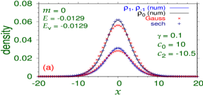
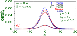
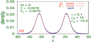
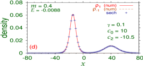
Figure 1: (Color online) Numerical (num) and analytic densities obtained with Gaussian (Gauss) and hyperbolic secant (sech) functions $\rho_{j},j=0,\pm 1$ of the three components for the lowest-energy overlapping ground-state vector soliton with $c_{0}=10$, $c_{2}=-10.5$, and $\gamma=0.1$ ($\gamma<\gamma_{c}=0.1768)$ for (a) $m=0,$ and (b) $m=0.4$. The same for the phase-separated two-component vector soliton in an excited state are shown in (c) and (d), respectively. The soliton profiles remain unchanged with a variation of $\gamma$ in the domain $0.1>\gamma>0$. Numerical ($E$) energy and variational ($E_{v}$) energy from sech ansatz are shown. The numerical energies displayed in plots (c) and (d) are larger than those in (a) and (b), respectively. All quantities in this and following figures are dimensionless.

III.1 Stationary solitons and their stability

The initial wave function in imaginary-time propagation is taken as the variational function (9) with the Gaussian form for the function $\phi(x)$ and with $\gamma=0$. To study the phase separation of the components of the vector soliton efficiently, it is appropriate to give a small separation between the positions of the $F_{z}=\pm 1$ initial state functions while maintaining $F_{z}=0$ component at the origin as

$$\Phi\equiv\left(\begin{array}[]{c}\phi_{+1}\\ \phi_{0}\\ \phi_{-1}\end{array}\right)=\frac{1}{2}\left(\begin{array}[]{c}(1+m)\phi(x+a)\\ \sqrt{2(1-m^{2})}\phi(x)\\ (1-m)\phi(x-a)\end{array}\right),$$ (39)

where $\phi$ is the normalized Gaussian function (10) and $a$ is a small number. If $\gamma<\gamma_{c}$, the critical value for phase separation, the $F_{z}=\pm 1$ components move to the center to form a fully overlapping three-component vector soliton in the final converged configuration. However, if $\gamma>\gamma_{c}$, the $F_{z}=\pm 1$ components move outwards to form a fully separated two-component vector soliton with the vanishing of the $F_{z}=0$ component. The imaginary-time propagation method prefers to maintain the symmetry of the initial state: overlapping or separated. By taking $a=0$ in Eq. (39) it is possible to find the overlapping excited state for $\gamma>\gamma_{c}$, where the ground state is phase separated; also by taking a large value of $a$ it is possible to find the phase-separated state for $\gamma<\gamma_{c}$, where the ground state is overlapping.

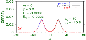
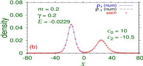
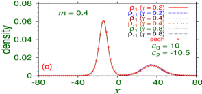
Figure 2: (Color online) Numerical (num) and analytic densities with the hyperbolic secant function (sech) $\rho_{j},j=\pm 1$ of the two components for the lowest-energy phase-separated vector soliton with $c_{0}=10$, $c_{2}=-10.5$, $\gamma=0.2>\gamma_{c}=0.1768$ for (a) $m=0,$ and (b) $m=0.2$, and (c) $m=0.4$. Numerical ($E$) energy and variational ($E_{v}$) energy from sech ansatz are shown.

We perform our calculation with the parameters $c_{0}=10$ and $c_{2}=-10.5$ (ferromagnetic), so that $c_{0}+c_{2}=-0.5<0$, to make the system attractive to have a vector soliton. The variational approximation in Sec. II.2 demonstrates that the present soliton profiles are determined entirely by the combination $(c_{0}+c_{2})$ of the interaction strengths $c_{0}$ and $c_{2}$, viz. Eqs. (13) and (16), which is also confirmed by our numerical calculation. Hence without losing generality, we consider in this section only positive values of $c_{0}$ in such a way that $c_{0}+c_{2}<0$. In this case the critical SO-coupling strength for phase separation (22) is $\gamma_{c}=0.1768$. In Figs. 1(a)-(b) we display the density of the components of the minimum-energy overlapping ground-state vector soliton for $\gamma=0.1$ $(\gamma<\gamma_{c})$ and for magnetization $m=0$ and 0.6, respectively. The result of the analytic variational approximation with the Gaussian and hyperbolic secant functions is also displayed in these plots. The variational results for the width $\alpha$ and $\sigma$ given by (13) and (16) are independent of magnetization $m$ and SO-coupling $\gamma$ and are the same for all components. The same is found to be true in the numerical calculation, in good agreement with the analytic approximation. In Figs. 1(c)-(d) we plot the densities of the phase-separated two-component vector soliton for the same parameters as in (a)-(b), respectively. In the case of the phase-separated two-component vector solitons, the analytic result cannot determine the positions of the component solitons, which have been introduced arbitrarily to fit the position of the components. In plots Fig. 1(a)-(d), the soliton profiles are practically unchanged for $0<\gamma<0.1$, although the energy is changing, viz. Eqs. (14) and (17). In Figs. 1(a)-(b) we find that the analytic results obtained with the hyperbolic secant function are superior to those obtained with the Gaussian function. Hence in the following we will only show the analytic results obtained with the hyperbolic secant function.

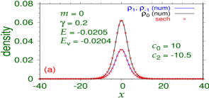
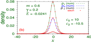
Figure 3: (Color online) Numerical (num) and analytic densities with the hyperbolic secant function (sech) $\rho_{j},j=0,\pm 1$ of the three components for the overlapping vector soliton in the excited state with $c_{0}=10$, $c_{2}=-10.5$, $\gamma=0.2>\gamma_{c}=0.1768$ for (a) $m=0,$ and (b) $m=0.6$. Numerical ($E$) energy and variational ($E_{v}$) energy from sech ansatz are shown.

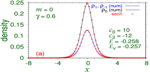
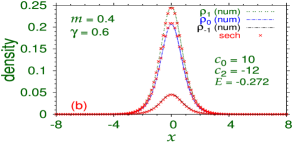
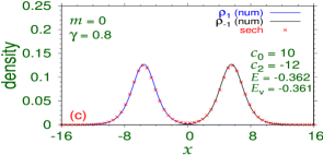
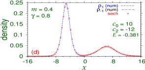
Figure 4: (Color online) Numerical (num) and analytic densities with the hyperbolic secant function (sech) $\rho_{j},j=0,\pm 1$ of the three components of the overlapping vector soliton in the ground state with $c_{0}=10$, $c_{2}=-12$, $\gamma=0.6<\gamma_{c}=0.7071$ for (a) $m=0,$ and (b) $m=0.4$. The same for the two components $\rho_{j},j=\pm 1$ of the phase-separated vector soliton in the ground state for $\gamma=0.8>\gamma_{c}$ and (c) $m=0,$ and (d) $m=0.4$. Numerical ($E$) energy and variational ($E_{v}$) energy from sech ansatz are shown.

In Figs. 2 we plot the densities of the phase-separated two-component minimum-energy ground-state vector soliton for $c_{0}=10,$ $c_{2}=-10.5$, and $\gamma=0.2>\gamma_{c}=0.1768$ for (a) $m=0,$ (b) $m=0.2,$ and (c) $m=0.4.$ and compare these with the analytic result from the hyperbolic secant function. To show that the density profiles for the phase-separated solitons are practically independent of the SO-coupling strength $\gamma$ ($\gamma>\gamma_{c}$), as predicted by the analytic relation (19), we exhibit in Fig. 2(c) the results for $\gamma=0.2,0.4$ and 0.8 in good agreement with each other.

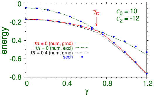
Figure 5: (Color online) Numerical (num) results of energy of $m=0$ ground- (grnd) and excited- (exci) state vector solitons versus SO-coupling strength $\gamma$, for interaction strengths $c_{0}=10$ and $c_{2}=-12$, displayed by full and dashed lines, respectively. The numerical results for for the $m=0.4$ ground-state vector solitons are shown by dashed-dotted line. The analytic results (sech) obtained with the hyperbolic secant function for the ground and excited states are displayed as solid circles. The analytic result is independent of $m$ and hence is the same for $m=0$ and $m=0.4$ vector solitons.

For $\gamma>\gamma_{c}$, the phase-separated two-component vector solitons are the ground states. while the overlapping three-component solitons become excited states. In Figs. 3 we exhibit the density profiles of these excited states for (a) $m=0$ and (b) $m=0.6$, respectively, and for $\gamma=0.2,c_{0}=10,c_{2}=10.5$. Although, these are excited states, the analytic results for energies and widths are in good agreement with the numerical energies.

To show the nature of the solitons with increased attraction we next consider $c_{0}=10,c_{2}=-12$ corresponding to a net attraction $c_{0}+c_{2}=-2$. As this net attraction increases, the width of the soliton reduces rapidly, viz. Eqs. (13) and (16), whereas the critical $\gamma_{c}$, viz. Eq. (22), increases. This is why we did not consider a larger value of $|c_{0}+c_{2}|$. In this case the critical SO coupling $\gamma_{c}=0.7071$. We display the densities of the overlapping ground states in Figs. 4 for (a) $m=0,\gamma=0.6$ and (b) $m=0.4,\gamma=0.6$ and compare these with the analytic counterparts. These densities remain practically unchanged for all $\gamma<\gamma_{c}$. For $\gamma>\gamma_{c}=0.7071$, the overlapping states become excited states and the densities of the phase-separated two-component ground states for $\gamma=0.8$ are shown in Fig. 4 for (c) $m=0$ and (d) $m=0.4$. The analytic results are found to be in good agreement with the numerical calculation.

We now study the evolution of the energy of ground- and excited-state vector solitons as a function of the SO-coupling strength $\gamma$, for interaction strengths $c_{0}=10,c_{2}=-12$. In Fig. 5, we display the numerical results for energy of the $m=0$ ground-state (full line) and excited-state (dashed line) vector solitons. For $\gamma<\gamma_{c}$, the critical SO-coupling strength for the formation of phase-separated two-component ground-state vector solitons, the ground-state solitons are the overlapping three-component solitons. For $\gamma>\gamma_{c}$, the ground state solitons are the phase-separated two-component solitons. The numerical results for the $m=0.4$ vector solitons are also displayed in this figure as dashed-dotted line. The analytic results for energy are independent of $m$ and are displayed by solid circles.

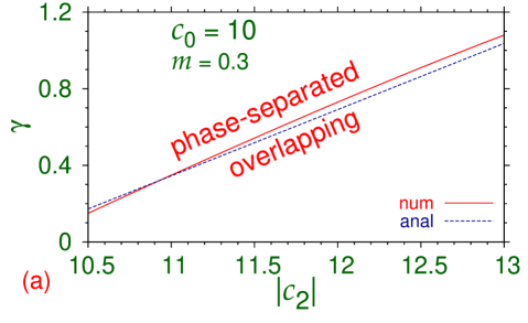
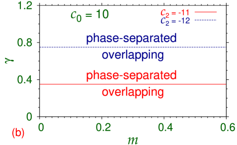
Figure 6: (Color online) (a) The numerical and analytic phase plot of phase separation in the $\gamma-|c_{2}|$ parameter space for $c_{0}=10$ and $m=0.3$. (b) The same in the $\gamma-m$ parameter space for $c_{0}=10$ and $c_{2}=-11,-12$. In this case the numerical and analytic results are very close to each other and only the former is shown.

The phase separation of the three-component vector soliton in parameter space is illustrated next for interaction strength $c_{2}$ and magnetization $m$ with the variation of SO-coupling strength $\gamma$. The analytic result depends on the interaction-strength combination $c_{0}+c_{2}$, whereas the numerical result should depend on both $c_{0}$ and $c_{2}$. In Fig. 6(a) we show the phase separation in the $\gamma-|c_{2}|$ parameter space for interaction strength $c_{0}=10$ and magnetization $m=0.3$. Both numerical and analytic results, in close agreement with each other, are shown. In Fig. 6(b) the numerical results of phase separation are illustrated in the $\gamma-m$ parameter space for $c_{0}=10$ and for $c_{2}=-11$ and -12.

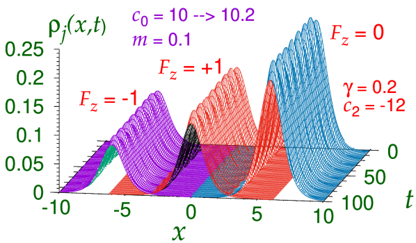
Figure 7: (Color online) Density profile of a vector soliton during real-time propagation demonstrating its dynamical stability. For a better view of the individual components, the component densities are plotted after a spatial displacement among these. The initial wave function was obtained by imaginary-time simulation with parameters $c_{0}=10,c_{2}=-12,m=0.1,\gamma=0.2$ and the real-time propagation was executed after changing $c_{0}$ to 10.2.

III.2 Dynamical stability and phase separation

To demonstrate that the vector soliton is dynamically stable we subject the ground-state vector soliton profile, obtained by imaginary-time simulation, to real-time propagation for a long time after giving a perturbation by changing the interaction strength $c_{0}$ slightly at time $t=0$. The profile of the vector soliton is very sensitive to $c_{0}$, viz. (13) and (16). For this purpose, we consider the overlapping vector soliton obtained with parameters $c_{0}=10,c_{2}=-12,m=0.1,\gamma=0.2$. The real-time propagation during 100 time units for this soliton was executed upon changing the interaction strength $c_{0}$ from 10 to 10.2 at time $t=0$. In Fig. 7 we exhibit the density profile of the three components of the vector soliton during real-time propagation. For a better view, we have displaced the density profile of components $F_{z}=-1$ and $F_{z}=0$ to $x=-5$ and $x=+5$, respectively, leaving the $F_{z}=+1$ component at $x=0$. The long-time stable propagation of the components of the vector soliton establishes its dynamical stability.

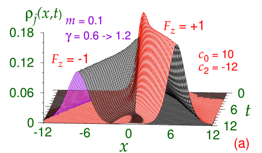
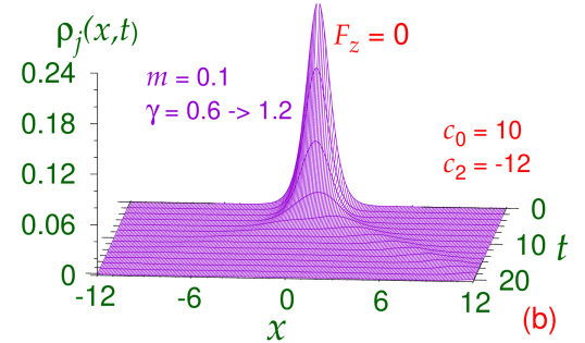
Figure 8: (Color online) Dynamics of phase separation of a three-component vector soliton upon changing the SO-coupling strength $\gamma$ from a value smaller than its critical value $\gamma_{c}$ $(=0.7071)$ for phase separation to a value larger than $\gamma_{c}$ by plots of densities of components (a) $F_{z}=\pm 1$ and (b) $F_{z}=0$ versus $x$ and $t$, obtained by real-time propagation. Employed parameters are $c_{0}=10,c_{2}=-12,m=0.1,\gamma_{c}=0.7071$, while $\gamma$ was changed from 0.6 to 1.2.

Next we demonstrate the dynamical phase separation of a three-component vector soliton. For this purpose we consider the ground-state three-component vector soliton profile soliton profile for $c_{0}=10,c_{2}=-12,m=0.1,\gamma=0.6$ obtained by imaginary-time propagation and subject it to real-time propagation upon changing $\gamma$ to 1.2. The initial $\gamma<\gamma_{c}=0.7071$ is appropriate for the formation of an overlapping three-component vector soliton in the ground state and the final $\gamma$ is appropriate for a phase-separated binary vector soliton in the ground state. In Figs. 8(a) and (b) we display the time evolution of density of the components $F_{z}=\pm 1$ and $F_{z}=0$, respectively. The components $F_{z}=\pm 1$ move away from each other while the component $F_{z}=0$ vanishes after time evolution as displayed in Figs. 8(a)-(b).

III.3 Collision of moving solitons

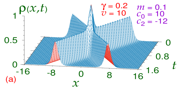
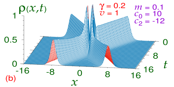
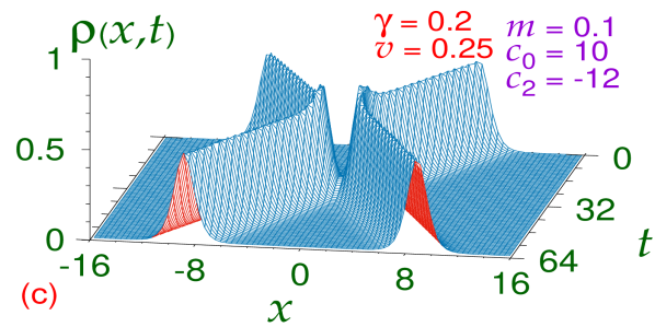
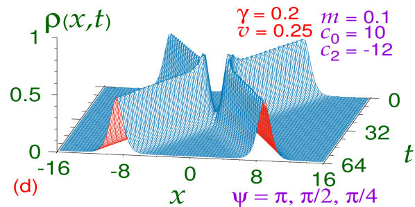
Figure 9: (Color online) (a) Elastic nature of collision dynamics of two vector solitons of Fig. 7 with $\gamma=0.2$ illustrated through a plot of total density $\rho(x,t)$, obtained by real-time propagation, versus $x$ and $t$. At $t=0$ individual solitons are placed at $x=\pm 8$ and set into motion in opposite directions with velocity $v=\pm 10$ by multiplying the imaginary-time wave functions of the two vector solitons by $\exp(\pm ivx)$, respectively. The same dynamics with (b) $v=\pm 1$ and (c) $v=\pm 0.25$. (d) The dynamics of (c) after introducing a relative phase $\psi=\pi,\pi/2,\pi/3$ or $\pi/4$ between the two vector solitons. Other parameters are $c_{0}=10,c_{2}=-12,\gamma=0.2,m=0.1$.

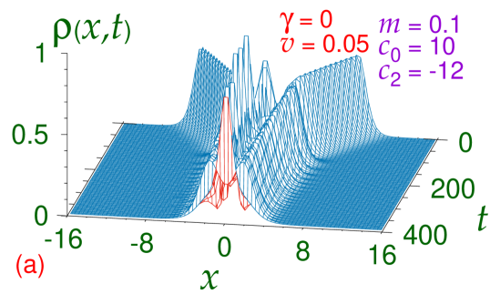
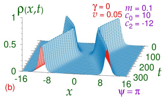
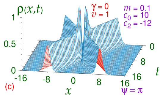
Figure 10: (Color online) (a) Inelastic collision dynamics resulting in soliton-molecule formation of two vector solitons of Fig. 7 with SO coupling switched off ($\gamma=0$) illustrated through a plot of total density $\rho(x,t)$, obtained by real-time propagation, versus $x$ and $t$. At $t=0$ individual solitons are placed at $x=\pm 8$ and set into motion in opposite directions with velocity $v=\pm 0.05$. (b) The dynamics of (a) with a relative phase $\psi+\pi$ introduced between the two vector solitons at $t=0$. (c) The dynamics of (a) with a velocity $v=1$ and a relative phase $\psi=\pi$ between the two vector solitons at $t=0$. Other parameters are $c_{0}=10,c_{2}=-12,\gamma=0,m=0.1$.

The dynamics of moving solitons is next studied by first generating the ground-state overlapping vector soliton numerically using imaginary-time propagation. The complex wave-function components, so obtained, are then multiplied by a complex phase $\exp(ixv)$, which are used as the initial states in real time simulation. The generated vector soliton is a moving soliton with velocity $v$ in the limit of very small space and time steps $dx$ and $dt$. In the following calculation the employed values of space and time steps are $dx=0.025$ and $dt=10^{-5}$, respectively. We will demonstrate that the present vector soliton can move without changing the density profile of the (three) components. The collision dynamics of scalar condensates depends referee on the relative velocity, relative amplitude, and relative phase $\psi$ of the two colliding solitons. In the present collision of SO-coupled vector solitons we find that the relative velocity has considerable effect on the collision process. However, the collision is reasonably insensitive to the relative phase $\psi$ and relative amplitude of the soliton components. To demonstrate the solitonic property of the overlapping vector soliton, we study the collision of two vector solitons each generated by imaginary-time propagation with parameters $c_{0}=10,c_{2}=-12,m=0.1,\gamma=0.2$. We take two vector solitons and place them at positions $x\equiv d=\pm 8$ and set them in motion in opposite directions with velocity $v=\pm 10$ (relative velocity of 20) so as to collide at $x=0$ after time $t=d/v=0.8$. During collision, the solitons are found to pass through each other essentially unchanged, and we study the collision dynamics. Both magnetization and normalization are conserved during propagation of a vector soliton resulting in the conservation of density profiles of each component. The density of each vector soliton is conserved after collision showing its elastic nature. This is displayed in Fig. 9(a) via a plot of total density $\rho(x,t)$ of the two vector solitons during collision. The two solitons emerge with the same velocity and the same total density after collision. However, the SO coupling generates a repulsion between the solitons and the situation changes at small velocities $v$ as illustrated in Figs. 9(b) and (c) at velocities $v=1$ and 0.25, respectively. The results of collision confirm a repulsion between the two SO-coupled vector solitons at small velocities and at small separation between them. For $v=0.25$ in Fig. 9(c), the repulsion due to SO-coupled repulsive interaction stops the two vector solitons from meeting each other; they come close at $t=d/v=32$, turn back and move away from each other with the same speed. This repulsion is also indicated for $v=1$ in Fig. 9(b), where the two vector solitons show a tendency to stay apart and not mix with each other. At all velocities, the two SO-coupled vector solitons emerge after collision without any visible deformation demonstrating the elastic nature of collision at all velocities.

To study the effect of relative phase of the two colliding vector solitons, we repeated the collision dynamics exhibited in Figs. 9(a)-(c) with relative phases of $\pi,\pi/2,\pi/3$ and $\pi/4$ between the two colliding vector solitons. The dynamics of Figs. 9(a)-(c) remains unchanged after the introduction of the relative phase demonstrating no effect of phase on the collision. In Fig. 9(d) we plot the collision dynamics of Fig. 9(c) after introducing the relative phase $\psi=\pi$ between the components at $t=0$. From Figs. 9(c)-(d) we find that the relative phase has no effect on the collision. The phases $\psi=\pi/2,\pi/3$ and $\pi/4$ were also found to yield the same dynamics. In case of usual scalar solitons, the effect of relative phase on collision dynamics is the maximum for $\psi=\pi$. The attractive interaction between two scalar solitons become repulsive upon the introduction of a relative phase of $\pi$ between the two colliding solitons referee .

To be sure that the small SO-coupled repulsive interaction $(\gamma=0.2)$ is causing the solitons to turn back and move away in Fig. 9(c), we studied the collision dynamics of vector solitons with the SO coupling interaction switched off. The resultant collision dynamics for a small velocity $v=0.05$ and SO coupling $\gamma=0$ is displayed in Fig. 10(a). In this case the vector solitons come close, meet each other at time $t=d/v=160$, and form a vector soliton molecule in an excited state which executes breathing oscillation and never separate showing the presence of an attraction between the two vector solitons. To study the effect of relative phase between the two vector solitons without SO coupling, we repeated the collision dynamics of Fig. 10(a) with a relative phase of $\pi$ between the two vector solitons and for $\gamma=0$ and the result is illustrated in Fig. 10(b). We consider a relative phase of $\pi$, as for this phase separation the effect of relative phase on collision dynamics is expected to be largest. In the phase-changed configuration there is a strong repulsion between the two vector solitons which keep them apart. As in the case of scalar solitons, the two vector solitons come close and turn back and emerge with the same speed without deformation as shown in Fig. 10(b). To see the effect of relative phase on velocity $v$, we consider in Fig. 10(c) the collision of the two solitons of Fig. 10(b) with an initial velocity $v=1$ and a relative phase $\psi=\pi$. Even at a larger velocity, when the effect of relative phase is expected to be less, the two vector solitons avoid each other because of the repulsion introduced by the relative phase.

IV Summary

We studied the generation, phase separation, and collision dynamics of overlapping three-component $(F_{z}=0,\pm 1)$ quasi-1D vector solitons of a SO-coupled spin-1 spinor ferromagnetic BEC ($c_{2}<0$) by a numerical solution and an analytic approximation of the mean-field GP equation, the SO coupling being of the form $\gamma p_{x}\Sigma_{z}$. The solitons appear for net interaction strength $(c_{0}+c_{2})<0$. The phase separation of the $F_{z}=\pm 1$ components takes place for the strength $\gamma$ of SO coupling $p_{x}\Sigma_{z}$ above a critical value $(\gamma>\gamma_{c})$, while the $F_{z}=0$ component vanishes. The vector solitons are demonstrated to be mobile and stable. By real-time simulation, we demonstrated the dynamical phase separation of an overlapping vector soliton upon increasing the strength of SO coupling above the critical value, viz. Fig. 8. At all velocities, the collision dynamics between two such vector solitons is found to be elastic with the conservation of the densities of each individual vector solitons, viz. Figs. 9. The vector solitons repel each other due to SO coupling and consequently, in collision at small velocities, the vector solitons come close to reach other and bounce back with same speed without ever meeting each other as shown in Fig. 9(c). The collision dynamics of two SO-coupled vector solitons is found to be insensitive to the relative phase between them. In the absence of SO coupling, in collision at small velocity the two vector solitons attract each other and form a vector soliton molecule in an excited state and never separate, viz. Fig. 10(a), quite similar to collision of two multi-component scalar solitons. Also, in the absence of SO coupling the collision dynamics is very sensitive to the relative phase, viz. Fig. 10(b). With the present experimental know-how, these vector solitons can be generated in a laboratory in a routine fashion and our predictions can be verified.

- (1) Y. S. Kivshar and B. A. Malomed, Rev. Mod. Phys. 61, 763 (1989); F. K. Abdullaev, A. Gammal, A. M. Kam- chatnov, and L. Tomio, Int. J. Mod. Phys. B 19, 3415 (2005).
- (2) K. E. Strecker, G. B. Partridge, A. G. Truscott, and R. G. Hulet, Nature (London) 417, 150 (2002); L. Khaykovich, F. Schreck, G. Ferrari, T. Bourdel, J. Cubizolles, L. D. Carr, Y. Castin, and C. Salomon, Science 256, 1290 (2002).
- (3) S. L. Cornish, S. T. Thompson, and C. E. Wieman, Phys. Rev. Lett. 96, 170401 (2006).
- (4) S. Inouye, M. R. Andrews, J. Stenger, H.-J. Miesner, D. M. Stamper-Kurn, and W. Ketterle, Nature (London) 392, 151 (1998).
- (5) V. M. Pérez-García and J. B. Beitia, Phys. Rev. A 72, 033620 (2005); S. K. Adhikari, Phys. Lett. A 346, 179 (2005); Phys. Rev. A72, 053608 (2005); L. Salasnich and B. A. Malomed, Phys. Rev. A 74, 053610 (2006).
- (6) D. M. Stamper-Kurn, M. R. Andrews, A. P. Chikkatur, S. Inouye, H.-J. Miesner, J. Stenger, and W. Ketterle, Phys. Rev. Lett. 80, 2027 (1998).
- (7) Y. Kawaguchi and M. Ueda, Phys. Rep. 520, 253 (2012).
- (8) V. Galitski and I. B. Spielman, Nature (London) 494, 49 (2013); J. Dalibard, F. Gerbier, G. Juzeliūnas, and P. Öhberg, Rev. Mod. Phys. 83, 1523 (2011); Y. Li, Giovanni I. Martone, and S. Stringari, Ann. Rev. Cold At. Mol. 3, Ch 5, 201 (2015) (World Scientific, 2015).
- (9) K. Osterloh, M. Baig, L. Santos, P. Zoller, and M. Lewenstein, Phys. Rev. Lett. 95, 010403 (2005); J. Ruseckas, G. Juzeliūnas, P. Öhberg, and M. Fleischhauer, Phys. Rev. Lett. 95, 010404 (2005); G. Juzeliūnas, J. Ruseckas, and J. Dalibard, Phys. Rev. A 81, 053403 (2010).
- (10) Y. A. Bychkov E. I. Rashba, J. Phys. C 17, 6039 (1984).
- (11) G. Dresselhaus, Phys. Rev. 100, 580 (1955).
- (12) Y.-J. Lin , K. Jiménez-García, and I. B. Spielman, Nature (London) 471, 83 (2011).
- (13) M. Aidelsburger, M. Atala, S. Nascimbène, S. Trotzky, Y.-A. Chen, and I. Bloch, Phys. Rev. Lett. 107, 255301 (2011); Z. Fu, P. Wang, S. Chai, L. Huang and J. Zhang, Phys. Rev. A 84, 043609 (2011); J.-Y. Zhang, S.-C. Ji, Z. Chen, L. Zhang, Z.-D. Du, B. Yan, G.-S. Pan, B. Zhao, Y.-J. Deng, H. Zhai, S. Chen, and J.-W. Pan, Phys. Rev. Lett. 109, 115301 (2012); C. Qu, C. Hamner, M. Gong, C. Zhang and P. Engels, Phys. Rev. A 88, 021604(R) (2013); A. J. Olson, S.-J. Wang, R. J. Niffenegger, C. -H. Li, C. H. Greene and Y. P. Chen, Phys. Rev. A 90, 013616 (2014).
- (14) Z. Lan and P. Öhberg, Phys. Rev. A 89, 023630 (2014); C. Wang, C. Gao, C.-M. Jian, and H. Zhai, Phys. Rev. Lett. 105, 160403 (2010)
- (15) J. Ieda, T. Miyakawa, and M. Wadati, Laser Phys. 16, 678 (2006); J. Ieda, T. Miyakawa, and M. Wadati, Phys. Rev. Lett. 93, 194102 (2004); L. Li, Z. Li, B. A. Malomed, D. Mihalache, and W. M. Liu, Phys. Rev. A 72, 033611 (2005); W. Zhang, Ö. E. Müstecaplioǧlu, and L. You, Phys. Rev. A 75, 043601 (2007); B. J. Dąbrowska-Wüster, E. A. Ostrovskaya, T. J. Alexander, and Y. S. Kivshar, Phys. Rev. A 75, 023617 (2007); E. V. Doktorov, J. Wang, and J. Yang, Phys. Rev. A 77, 043617 (2008); B. Xiong and J. Gong; Phys. Rev. A 81, 033618 (2010); P. Szankowski, M. Trippenbach, E. Infeld, and G. Rowlands, Phys. Rev. Lett. 105, 125302 (2010); M. Mobarak and A. Pelster, Laser Phys. Lett. 10, 115501 (2013); O. Topic, M. Scherer, G. Gebreyesus, et al., Laser Phys. 20, 1156 (2010); M. Guilleumas, B. Julia-Diaz, M. Mele-Messeguer, and A. Polls, Laser Phys. 20, 1163 (2010).
- (16) Y. Xu, Y. Zhang, and B. Wu, Phys. Rev. A 87, 013614 (2013); S. Cao, C.-J. Shan, D.-W. Zhang, X. Qin, and J. Xu, J. Opt. Soc. Am. B 32, 201 (2015); H. Sakaguchi and B. A. Malomed, Phys. Rev. E 90, 062922 (2014); Lin Wen, Q. Sun, Yu Chen, Deng-Shan Wang, J. Hu, H. Chen, W.-M. Liu, G. Juzeliūnas, Boris A. Malomed, and An-Chun Ji, Phys. Rev. A 94, 061602(R) (2016); V. Achilleos, D. J. Frantzeskakis, P. G. Kevrekidis, and D. E. Pelinovsky, Phys. Rev. Lett. 110, 264101 (2013).
- (17) Y.-K. Liu and S.-J. Yang, Europhys. Lett., 108, 30004 (2014); Decheng Ma and Chenglong Jia, Phys. Rev. A 100, 023629 (2019); Yan-Hong Qin, Li-Chen Zhao, and Liming Ling, Phys. Rev. E 100, 022212 (2019).
- (18) S. Gautam and S. K. Adhikari, Laser Phys. Lett. 12, 045501 (2015).
- (19) S. Gautam and S. K. Adhikari, Phys. Rev. A95, 013608 (2017).
- (20) S. Gautam and S. K. Adhikari, Phys. Rev. A97, 013629 (2018).
- (21) Y. Li, G. I. Martone, L. P. Pitaevskii, and S. Stringari, Phys. Rev. Lett. 110, 235302 (2013); G. I. Martone, Y. Li, L. P. Pitaevskii, and S. Stringari, Phys. Rev. A 86, 063621 (2012).
- (22) Y. Zhang and C. Zhang, Phys. Rev. A 87, 023611 (2013); G. I. Martone, F. V. Pepe, P. Facchi, S. Pascazio, and S. Stringari, Phys. Rev. Lett. 117, 125301 (2016).
- (23) L. Salasnich, A. Parola, and L. Reatto, Phys. Rev. A 65, 043614 (2002).
- (24) S. Gautam and S. K. Adhikari, Phys. Rev. A91 , 013624 (2015).
- (25) S. Gautam and S. K. Adhikari, Phys. Rev. A 90, 043619 (2014).
- (26) S. Gautam and S. K. Adhikari, Phys. Rev. A 92, 023616 (2015).
- (27) T. Ohmi and K. Machida, J. Phys. Soc. Jap. 67, 1822 (1998); T.-L. Ho, Phys. Rev. Lett. 81, 742 (1998); S. Yi, Ö. E. Müstecaplioǧlu, C. P. Sun, L. You, Phys. Rev. A 66, 011601(R) (2002).
- (28) P. Muruganandam and S. K. Adhikari, Comput. Phys. Commun. 180, 1888 (2009).
- (29) D. Vudragović, I. Vidanović, A. Balaž, P. Muruganandam, and S. K. Adhikari, Comput. Phys. Commun. 183, 2021 (2012).
- (30) L. E. Young-S., D. Vudragović, P. Muruganandam, S. K. Adhikari, and A. Balaž, Comput. Phys. Commun. 204, 209 (2016); L. E. Young-S., P. Muruganandam, S. K. Adhikari, V. Lončar, D. Vudragović, and A. Balaž, Comput. Phys. Commun. 220, 503 (2017).
- (31) F. Y. Lim and W. Bao, Phys. Rev. E 78, 066704 (2008).
- (32) J. P. Gordon, Opt. Lett. 8, 596 (1983).